
ATMP-CA: Optimising Mixed-Criticality Systems Considering Criticality Arithmetic


Department of Computer Science, University of Hertfordshire, Hatfield AL10 9AB, UK
*
Authors to whom correspondence should be addressed.
Electronics 2021, 10(11), 1352; https://0-doi-org.brum.beds.ac.uk/10.3390/electronics10111352
Submission received: 27 April 2021
/
Revised: 19 May 2021
/
Accepted: 31 May 2021
/
Published: 6 June 2021
(This article belongs to the Special Issue Emerging Advances for Cyber-Physical Systems)
Abstract
:Many safety-critical systems use criticality arithmetic, an informal practice of implementing a higher-criticality function by combining several lower-criticality redundant components or tasks. This lowers the cost of development, but existing mixed-criticality schedulers may act incorrectly as they lack the knowledge that the lower-criticality tasks are operating together to implement a single higher-criticality function. In this paper, we propose a solution to this problem by presenting a mixed-criticality mid-term scheduler that considers where criticality arithmetic is used in the system. As this scheduler, which we term ATMP-CA, is a mid-term scheduler, it changes the configuration of the system when needed based on the recent history of deadline misses. We present the results from a series of experiments that show that ATMP-CA’s operation provides a smoother degradation of service compared with reference schedulers that do not consider the use of criticality arithmetic.
1. Introduction
Mixed-criticality systems are a special kind of safety-critical systems where not all provided services have the same criticality. For example, in an aeroplane, the correct operation of the engines is of higher criticality than the onboard intercom system. With the seminal work by Vestal in 2007 [1], scheduling of mixed-criticality systems became an active research field [2,3,4,5,6,7,8].
Developing and assuring higher-criticality services requires more effort than developing services at a lower criticality [9]. Criticality arithmetic, also referred to as SIL arithmetic, is a common, if informal, method to reduce that effort [10] by combining multiple independent redundant lower-criticality services or components to realise a single higher-criticality service. Should any one of these components fail, the others, being independent, will continue to provide this service. This means that the overall service can be assured for the necessary higher criticality without the need to assure any one single component of this higher criticality.
Criticality arithmetic has a number of benefits, as identified in Section 3.2.1. These largely include the reduced development and assurance costs as a result of each individual component being of lesser importance to safety than it might be otherwise. However, there are also a number of drawbacks, as discussed in Section 3.2.2. In particular, criticality arithmetic can make it more difficult to adequately determine the impact of individual component failures.
The use of criticality arithmetic is an informal and qualitative process with no formal universally accepted definition. In this paper, we examine how the use of criticality arithmetic in a system can impact mixed-criticality task scheduling for that system.
Specifically, we present a mixed-criticality scheduler that takes into account information about where criticality arithmetic has been used in the system. Our example is based on the ATMP scheduler from Iacovelli et al. [11]. This scheduler provides better handling of tasks that are replicated for criticality arithmetic compared with a similar reference without awareness of criticality arithmetic. This amended ATMP scheduler, ATMP-CA, takes the utility functions as input for each task, so that the overall system utility can be gracefully distributed among tasks in case of resource shortages, e.g., caused by faults [12,13].
The remainder of the paper is structured as follows: Section 3 describes criticality arithmetic in further detail with a link to safety standards. Section 4 describes the system model that is used for the criticality-arithmetic-aware ATMP-CA, described in Section 5. An experimental evaluation is provided in Section 6. Section 7 concludes this paper. Finally, a glossary of the symbols of the system model and a list of acronyms are provided in Appendix A and Appendix B.
2. Related Work
Vestal triggered the research on mixed-criticality scheduling with his seminal paper on that topic [1]. Fundamental to his discussion was the assumption of resource shortages caused by underestimations of the real WCET of tasks. Considerable research on mixed-criticality that followed also focused on that specific cause of a resource shortage. With ATMP-CA, we are able to consider any source of resource shortage, i.e., we do not limit the type of faults to overruns of WCET estimates.
Baruah et al. discussed methods to tolerate a minimal number of WCET underestimations, allowing the system to maintain full utility up to a certain number of WCET estimate overruns [14]. Again, ATMP-CA differs in that it does not restrict the source of the resource shortage of WCET estimate overruns, and it is capable of taking into account information about criticality arithmetic.
Jiang et al. highlighted the gap between mixed-criticality theoretical models and industrial standards [15], the cause of which is that implementing theoretical models in industry is difficult due to the absence of industrial safety standards considerations during the development of these models. The authors narrowed this gap by extending the widely used mixed-criticality model, adaptive mixed criticality (AMC) [16], into a generic industrial architecture (Z-MC) that considers industrial safety standards. Z-MC provides runtime safety analysis with sufficient isolation between critical and non-critical services using a flexible model that can be integrated with different safety standards.
ATMP-CA differs from all the works described above in that it does not restrict the source of resource shortages in WCET estimate overruns, and it is capable of considering information about criticality arithmetic.
Kadeed et al. introduced online reconfiguration mechanisms to be used in case of foreseen core failures, while ensuring sufficient isolation according to safety standards between critical and non-critical services during the reconfiguration process [17]. The mechanism assumes continuous monitoring for service degradation is available, and identifies a foreseen core failure if services degradation exceed the hazardous level. Hence, services are replicated/copied to other cores rather than moving them since the detection occurs before the core failure. However, service replication relies on plans provided for the reconfiguration process. Similar to ATMP-CA, Kadeed et al. allowed for other faults than the original Vestal model, i.e., core failures. However, they did not include a system utility optimisation as provided by AMTP-CA, nor did they consider criticality arithmetic.
Iacovelli et al. developed a mid-term mixed-criticality scheduler [11], called ATMP. As a mid-term scheduler, ATMP performs scheduling decisions not at the granularity of task arrival/completion, but rather after a period of observation, to adjust the system load appropriately. ATMP is the closest method to ATMP-CA. Whereas ATMP is agnostic to information about the use of criticality arithmetic in the system, we used ATMP as inspiration for the ATMP-CA scheduler, developed in this article. ATMP-CA shares many characteristics with ATMP, but has a different utility optimisation system to consider. information about criticality arithmetic
3. Criticality Arithmetic
Although a formal definition of criticality arithmetic does not exist, in this section, we describe some practical aspects of its application.
3.1. Safety Integrity Implementations
The safety integrity of components or modules is an important concept across multiple domains, including the nuclear [9], the automotive [18], and civil aviation [19] fields. The standards associated with each of these fields identify terminology for denoting the safety integrity of a component, including safety integrity levels (SILs), in IEC 61508, automotive safety integrity levels (ASILs) in ISO 26262, and development assurance levels (DALs) in ARP 4654. In this section, we provide a brief introduction to safety integrity, using the SIL terminology of IEC 61508 [9] as an example. Further details can be found in [10].
IEC 61508 [9] defines the safety integrity of a component as the probability of that component satisfactorily performing its specified safety function. It defines four SILs, with a higher safety integrity level being ascribed to components that are more important to safety. In this way, the SIL of a component is an indication of the extent to which that component is important with regard to the safety of the overall system. As an indication, Table 1 provides the association between the target failure rate of a component (the probability of failure on demand (PFD) or, for continuous operations, the probability of failure per hour (PFH)) and the consequent associated SIL of that component, as described in [9].
In more detail, the SIL assigned to a component provides information about the level of rigour expected when developing that component. Generally, development and validation of a component to a higher SIL require more rigour than development of that component to a lower SIL. Specific details of the required development activities at each SIL are provided in [9], and cover areas including test coverage, coding practices, and acceptability of documentation. It is important to note that using the development techniques recommended for a particular SIL does not guarantee the achievement of a given failure rate. That is, Table 1 should be used only for determining the SIL based on the required failure rate and not to claim satisfaction of a target failure rate based on the use of specified development techniques.
3.2. Criticality Arithmetic and Safety Integrity
Criticality arithmetic (or SIL arithmetic as termed in [10]) refers to the practice of using multiple redundant independent implementations of a lower integrity level component providing a function F, in order to realise F at a higher integrity level than that of any of the individual components [20]. Criticality arithmetic therefore relies on the use of functional redundancy, or the duplication of certain critical system components that all provide a defined function. This means that if any one of these components fails, the remaining components will be able to provide that function.
Different fields use of this concept with their own specific integrity terminology. In IEC 61508 [9], SIL arithmetic is used when discussing how hardware systems of different SILs can be combined and in determining the SIL of the resultant combined system. Where a safety function is implemented via multiple channels with a given hardware fault tolerance, IEC 61508 defines that the overall SIL is calculated by identifying the channel with the highest SIL and adding a number of integrity levels dependent on the hardware fault tolerance of the combined channels.
Similarly, ISO 26262 [18] identifies ASIL decomposition as a process permitting a safety function assigned a nominated ASIL to be decomposed into redundant safety requirements, satisfied by independent architectural elements. This is most often used to decompose a safety requirement into a functional requirement and a safety mechanism acting against the failure of that functionality.
ARP 4754 [19] also uses criticality arithmetic within the civil aviation field. This standard permits the establishment of functional failure sets with multiple members, where the development assurance level (DAL) assigned to these members is permitted to be lower than the DAL assigned to the top-level failure condition.
In all these examples, we note that there is a limit to the extent of the criticality arithmetic that can be performed, i.e., to the consequent increase in criticality of the top-level component as a result of leveraging redundancy at lower levels. We further note that an effective system of redundancy management [21] is required in order to detect primary component failure and to reconfigure the system to use the redundant component in place of the primary component. Effective redundancy also requires independence of the redundant components such that multiple components will not be affected, for example, by a common mode failure. Systems with built-in redundancy can continue to operate, in some cases up to several days [22], in the event of partial failure.
3.2.1. Benefits of Criticality Arithmetic
It is generally regarded as less resource-intensive to develop components at lower integrity levels, as the development and validation processes are correspondingly less rigorous. This is discussed in more detail in Section 3.1. As a result, employing criticality arithmetic in system development can provide benefits in terms of both reduced development time and reduced development cost. However, demonstrating sufficient independence between these relevant components may still be a non-trivial task [23]. Criticality arithmetic also allows for the commercial pressures of developing and procuring systems. In some industries, logistical factors mean that components have to be procured before their integrity levels can be assured. Should these components be later shown to have achieved a lower integrity level than that expected, criticality arithmetic may be used to address the gap. Similarly criticality arithmetic can, in some cases, permit the use of legacy components (i.e., where the development effort is already completed) at lower integrity levels [24].
Criticality arithmetic permits the use of less-complex components, where these have achieved a lower SIL than that needed by the overall system. Components of lower complexity are easier to develop, as well as typically being easier and cheaper to maintain. Moreover, their use can reduce the risk of an undetected failure mode.
3.2.2. Drawbacks of Criticality Arithmetic
Although the use of criticality arithmetic may confer benefits as described in Section 3.2.1, it can also lead to conflicts in determining the impact of system or component failures.
Given a system where two or more redundant components are linked via criticality arithmetic to provide a service, a failure of one of these components eliminates the “protective” element of redundancy. Consequently, the entire service can no longer be adequately assured at the higher integrity, being now provided only by a single component of lower integrity.
This is of particular relevance where the integrity of the multiple redundant independent components (i.e., the SIL, DAL, and ASIL) is used as the input to a mixed-criticality task scheduler. Mixed-criticality scheduling allows for tasks of higher criticality to be given preference when resources are scarce. An example of such a scheduler is introduced in Section 5.
Informally, this means that, where necessary, the tasks most important to safety are prioritised over tasks of lesser importance to safety. However, if one of the components in the set providing a function F at higher integrity than that of the individual components (via criticality arithmetic) was to fail, the other components in this set would have to be given greater preference by the task scheduler if F is to be maintained at the required integrity level.
A second issue relevant to scheduling is the case of multiple dependent (but not redundant) components working together to implement a service. In this situation, a failure in one of these components may result in a failure of the overall service since an important part of the sub-goal would be no longer achievable. A mixed-criticality scheduler may therefore choose to abandon all the related tasks implementing the entire service.
4. System Model
In the following, we describe our system model and assumptions. We assume a mixed-criticality system, which consists of multiple services that can have different levels of criticality. A service can be implemented by one task or multiple tasks using criticality arithmetic. The system provides a number of services:
- is the service’s name.
- l
- is the service’s criticality level, with . A higher value of means a higher level of criticality. The vector is used to represent all possible criticality levels in a system: , with being the minimum and being the maximum possible criticality level.
- T
- is the set of tasks that implement the service s. If only one task implements the service (), then no criticality arithmetic is used, and the task in this case has the same criticality as the service.If multiple tasks implement the service (), then criticality arithmetic is used: All the tasks implement the same service s with redundant execution. The criticality of each is less than the criticality of service s it implements.
Each task of a task set T is defined as follows:
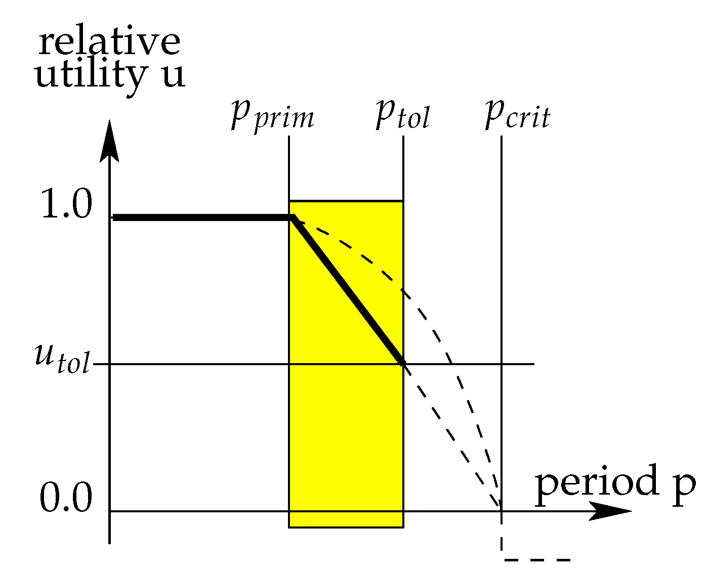
- is the utility function of task . The input parameter of the utility function is the chosen period, i.e., throughput. The utility function is characterised by the following properties: . is the primary period, with the relative utility being 1.0 up to this period. At the tolerance period , the resulting utility is , with the utility linearly interpolated between and .
- s
- is the service that is implemented by task .
- d
- is the relative deadline of task . We assume implicit deadlines, e.g., . (Note that this assumption is only chosen for the scheduling test in our implementation, but it is not a requirement of our optimisation method.)
- c
- is the WCET estimate of task . Depending on the underlying short-term scheduling protocol, the WCET estimate can be different for each criticality level. However, the mid-term scheduler described in this paper does not require this.
- l
- is the criticality level of task with . A higher value of l indicates a higher level of criticality. The vector is used to represent all possible criticality levels in a system: , with being the minimum and being the maximum possible criticality level.
- represent the task’s chosen period and the resulting utility u, respectively. The period p can be chosen within the tolerance interval: . The resulting utility is defined by the task’s utility function: . Section 4.1 We also use an absolute utility, U, which is calculated as .
The aim of the method described in this paper is to find a period for each task so that the overall system utility is maximised.
The individual instances of a task at runtime are called jobs. A job j is described by the following tuple:
where a is the arrival time and is the actual execution time. The entry refers to the task this job is instantiated from.
4.1. TRTCM
The fundamental concept of our scheduler is the tolerance-based real-time computing model (TRTCM) [13,25]. Instead of using a single performance limit such as a deadline or throughput limit, in TRTCM, a tolerance range is added, which allows a guided search for the best overall system utility in case of resource shortages.
In this paper, we focus on optimising the throughput of a system based on TRTCM. For any period , the relative utility is 1.0, i.e., the maximum. For any period higher than , the relative utility of a service degrades. This degradation is approximated by the utility function of a service, which defines another period up to which the service is still considered acceptable but with lower utility . For any period , the relative utility is expressed as a linear function, as shown in Figure 1.
The utility u of a task is calculated from its period p. The periods of all tasks are adjusted such that the overall system utility if maximised under the given resource constraints. For example, if some of the computing cores fail, then the system will have a significantly lower utility. However, with the help of the utility functions, the degradation can be performed in a graceful way.
4.2. Computing Elements
The platform model consists of multiple computing elements we call cores . For our purpose, istdoes not matter whether these cores are part of a multi-processor CPU or are on separate CPUs. The central objective is to optimise the system utility over all cores with potential resource shortages.
We also model a notion of computing capacity for each core . The computing capacity is linked to the worst-case execution time (WCET) of a task , as the WCET is based on a reference computing capacity we denote as . If another core has a computing capacity of , i.e., running twice as fast as the reference core, then the effective WCET of a task running on that cores would be . As such, we can model, for example, the case of different cores running with different clock frequencies.
The total computing capacity of the whole system can be calculated as
This platform model allows the precise modelling of platforms with homogeneous cores. In case of non-homogeneous cores, it would be better to use a different WCET of a task for each core .
5. ATMP with Criticality Arithmetic
The adaptive tolerance-based mixed-criticality protocol (ATMP) [11] is an application of the TRTCM [13,25] that maximises the system utility on each core by adjusting the periods of tasks within their tolerance range. The basic implementation of ATMP categorises system tasks according to their adaptation capability. In other words, the ability of a task to relax its interarrival rates, and its usefulness to the overall system decides if it will be allocated or not in the case of a omputing resource shortage. In this case, ATMP sort tasks according to decreasing criticality. Then, a critilcality-utility-aware allocation for system tasks is performed on available cores. On each core, if the partitioned tasks on that core is schedulable, then it is processed by the underlying scheduler. Otherwise, a binary search heuristics with integer linear programming (ILP) is performed to optimise the task set periods. The optimisation process maximises the overall system utility through maximising the utility of individual tasks by exploiting their safety margins. However, if no feasible solution is found for the whole task set, ATMP drops the tasks with the least criticality in each step of the binary search according to their adaptation capability.
Our modification of ATMP consists of the criticality-arithmetic-aware allocation of tasks to computing cores, and an adaptation for the ILP objective function to consider different contexts of replicated tasks implementing a service based on criticality arithmetic.
5.1. Criticality-Arithmetic-Aware Allocation to Cores
The task allocation to cores in ATMP-CA differs from the original in ATMP by avoiding more than one of the replicated tasks from a service with criticality arithmetic being allocated to the same core. The reason for this is simply to ensure fault tolerance for the replicated tasks, so that each core failure can disrupt at maximum one of the replicated tasks. In addition, the new core allocation also drops task replicas if there are more task replicas for one service than there are cores available. By dropping these replicas, we avoid blocking computing resources on a core for no benefit.
Algorithm 1 shows the implementation of the core allocation in ATMP-CA. The algorithm has two input parameters: , the list of all tasks, pre-sorted with decreasing criticality; and , the list of all cores available for allocation. The outer while-loop from lines 2–12 runs as long as there are tasks in . On line 3, the function removes the task with maximum criticality from . On line 4, the list with all core IDs is copied as . This copy is needed in case of replicated tasks to ensure that no two replicated tasks of the same service occurr on the same core. On line 5, the function removes the core with the currently minimum task load assigned from the core list . Lines 6–8 check whether the task already has a replica on the core . If this is the case, then inside the loop, a new core is extracted from until either a core is found that has no replica of allocated or all cores have been tried without success. Lines 9–11 register the allocation of the task to core only if the previous search for the core without a replica already allocated was successful. If this search was unsuccessful, then task is simply dropped and not allocated to a core. This search can only fail if there are fewer operational cores available than the number of task replicas with which services using criticality arithmetic are implemented.
| Algorithm 1: Criticality-arithmetic-aware allocation of tasks to cores. |
 |
When Algorithm 1 terminates, each of the tasks in the task set has been either allocated to a core or has been dropped. The purpose of this allocation is to assign the tasks to a core. Later, within each core, as part of the utility optimisation, which is the same as in ATMP [11], some tasks might be removed again from a core in order to pass the schedulability test.
5.2. Formulation of ILP Problem for ATMP-CA
In this section, we describe the ILP formulation to find the optimal task periods. We describe the constants and variables of that ILP problem, the goal function to optimise the system utility, and the different constraints that have to be considered.
- Optimisation parameters (constants): In ATMP, the units of scheduling are tasks. As described in Section 4, each task of a task set T consists of the following components:where the utility function is characterised by the following properties: . We model the utility function and the criticality of each task in the ILP problem with the following constants:
| the WCET of , | |
| the primary period (with utility ), | |
| the tolerance period, | |
| the utility at the tolerance period , | |
| the criticality weight of , | |
| the computing capacity of . |
- The parameters , , and characterise a task’s utility function by two linear lines, as shown in Figure 1. The horizontal line is a constant utility of , which can be directly expressed as an ILP constraint. The sloped line of each task’s utility function can be also derived from , , and , for which we have to calculate its slope and y-intercept to express it as a line equation:
- Optimisation variables: We use the following optimisation variables to find the optimised task configurations:
| the chosen period of task , | |
| the relative utility of task . |
- Objective function The optimisation ILP goal function maximises the system utility through maximising the utility variable of each task multiplied by its criticality weight :The criticality weight is explained below under the optimisation constraints.
- Optimisation constraints We express the piecewise affine approximationsof the utility functions to the following constraints:
- The resource constraints are used to limit the workload of each of the available cores . The maximum workload a core is its computing capacity :
- The tolerance constraints determine the maximal acceptable period of
- In ATMP, the weight is always set to the criticality of a task . In contrast, in ATMP-CA, the calculation of the weight of a task depends on the context with the replicas on other cores. In ATMP-CA, the is only set to the criticality of the task in the case where another replica of the task has already been allocated with its maximum utility or there is another replica of the task allocated in the cores still to be processed. Otherwise, the weight is set to the criticality of the service it implements, which is higher than .
- The implementation of the ILP formulation in ATMP-CA to calculate the weight is shown in Algorithm 2. The algorithm has a single input, the task , for which we want to calculate the weight , as used in Equation (4). On line 2, function determines whether a replica of task has been optimised with maximum utility in already-processed cores, and function checks whether the not-yet processed cores included an allocation of a replica of task . If one of these two functions returns , then we choose the task’s criticality on line 3. Otherwise, we choose on line 4 the criticality of the task’s service . On line 7, the weight for the ILP objective function is set to the determined criticality l.
6. Experiments
In the following, we describe the setup and results of our experiments.
| Algorithm 2: Calc-CA-aware ILP-weight. |
 |
6.1. Setup of Experiments
We implemented an ATMP-CA scheduling simulator as described in Section 5. We configured the simulator to simulate a multi-core system with 10 cores, where we simulated fault scenarios by making 10, 4, or 2 cores out of the 10 cores available. As such, we simulated the resulting overall system utility for different cases of resource shortages. In addition to the ATMP-CA protocol, this simulator implemented the ATMP and SAMP protocols for reference, as described in [11]. In essence, ATMP is similar to ATMP-CA in the sense that it also performs utility optimisation, but its core allocation and ILP constraints for utility maximisation do not take into account any of the services using criticality arithmetic. So, the comparison of ATMP-CA and ATMP shows the potential benefit of supporting any knowledge about criticality arithmetic in the scheduler. The other scheduler, SAMP, is generally less capable than ATMP and is only included for further reference. We then implemented another protocol, SAMP-CA, which is basically the simple SAMP protocol, but using the new Algorithm 1 for core allocation, which is also uses knowledge about criticality arithmetic. As such, SAMP-CA might perform better for systems with criticality arithmetic than SAMP, but it is not supposed to be able to compete with the utility optimisation performed by ATMP-CA.
We generated a task set with random parameters for worst-case execution time c and utility function . The implicit deadlines d were chosen to be equal to the primary period . The criticality of a task or service was either HI or LO, which correspond to a numeric value of either 2.0 or 1.0, respectively. We constrained the task generation such that it included two normal HI services (S1 and S2), two HI services that use criticality arithmetic (S3 and S4), and a few other LO services (S5, S6, S7, and S8). The whole structure of this task set is shown in Table 2. As shown in the table, the tasks T1 and T2, which implement the HI services S1 and S2, have the same criticality as the service. However, the HI services S3 and S4, which use criticality arithmetic, are both implemented by two redundant tasks T3a and T3b, and T4a and T4b, respectively, which all have LO criticality.
6.2. Results of Experiments
Figure 2 shows the results for our experiments with either 10, 4, or 2 cores out of 10 cores available. The MAX line denotes the maximum possible absolute utility for each task, which was either 2.0 or 1.0.
This case represents the optimal allocation, which means that for each task, it was possible to assign them their primary period , resulting in the maximum relative utility of 1.0, and no service was dropped.
Here, SAMP allocated the tasks of all HI-criticality services S1, S2, and S4 to cores, except the two LO-criticality task replicas T4a and T4b that implement service S3, whereas SAMP-CA allocated all HI-criticality tasks to cores at the cost of dropping all LO-criticality tasks. Though both SAMP and SAMP-CA showed an equivalent number of allocated and dropped tasks, they differed in the behaviour of dropping tasks belonging to services with criticality arithmetic. For ATMP and ATMP-CA, both protocols successfully allocated all services to cores, with a slight degradation in their absolute utility without dropping any tasks. The effect of the criticality-arithmetic-aware generation of the ILP objective function is described in Section 5.2, in this case, for service S3. With ATMP-CA, the first task T3a was set to full utility, resulting in the degraded utility of T3b, which allowed allocating resources to other tasks. Since both tasks implemented the same service S3, there was no need to allocate both of them at maximum utility when the system experienced an overload, as seen by the classical ATMP. A similar effect was seen with service S4, where ATMP-CA allowed a degraded utility for task T4a and then allocated full utility to T4b, whereas with ATMP, both tasks of S4 were degraded.
Figure 2c shows the case with 2 out of 10 cores available. Here, SAMP retained the tasks of HI-criticality services S1 and S2 and just one LO-criticality task T8, but dropped all the tasks of other HI-criticality services, including S3 and S4. SAMP-CA performed a bit better by retaining the tasks of HI-criticality services S1 and S2 and retaining one task T4b of HI-criticality service S4, while dropping all other services. This shows that the criticality-arithmetic-aware core allocation in SAMP-CA provides some benefit, but generally both SAMP and SAMP-CA have limited performance, as they do not support flexibility within the tolerance range. ATMP and ATMP-CA showed the significant difference of dropping HI-criticality services. ATMP retained two HI-criticality services and four LO-criticality tasks but dropped both S3 and S4 replicas, whereas ATMP-CA successfully allocated all HI-criticality services, including the replicated tasks, and dropped all LO-criticality ones. In addition, ATMP-CA allocated the S3 replica task D with the maximum utility as a result of the degradation of task C, and both S4 replicas were degraded, which showed that the modified optimisation process could not find a solution to allocate task F at maximum utility.
6.3. Discussion
The aim of the experiments was to show the benefit of taking into account knowledge about criticality arithmetic in the design of a mixed-criticality scheduler. The experiments showed that the criticality-aware core allocation in ATMP-CA and SAMP-CA provides a benefit over ATMP and SAMP, respectively, by ensuring that tasks from services using criticality arithmetic are allocated to separate cores. The modified ILP objective function of ATMP-CA was found to better use resources in case of resource limitations. Overall, ATMP-CA allows an even smoother degradation compared with ATMP in the case of services using criticality arithmetic.
The limitation of the current experiments is that we only examined systems with two criticality levels. Future work may involve extending the method to multiple levels of criticality.
7. Conclusions
In this paper, we described the concept of criticality arithmetic, also known as SIL arithmetic, which is a technique used to reduce the required development effort of a service using task replication. The contribution of this paper is the development of ATMP-CA, a mid-term scheduler that takes into account information about criticality arithmetic to provide a graceful degradation of system utility in the case of resource shortages, for example, those caused by faults. As such, ATMP-CA can optimise the overall system utility in the case of resource shortages, with special consideration of services implemented via criticality arithmetic. Although it is common to limit the source of resource shortages in mixed-criticality systems to overruns of WCET estimates, we were able to consider any source of resource shortage, including failure of computing elements.
We conducted experiments comparing ATMP-CA with ATMP and the simpler scheduler SAMP. The results showed that ATMP-CA is capable of serving systems with criticality arithmetic better than the others. For example, ATMP-CA was the only scheduler that was able to retain service S3 with criticality arithmetic in case where 8 out of 10 cores failed. In the case where 6 out of 10 cores failed, both ATMP-CA and SAMP-CA (an extension of SAMP with the same core allocation as ATMP-CA) were able to retain service S3 with criticality arithmetic. The latter case showed that considering criticality arithmetic during the core allocation is important on its own for criticality arithmetic.
Author Contributions
Motivation of criticality arithmetics: C.M.; design of the ATMP-CA method: S.F. and R.K.; implementation: S.F.; supervision: R.K. All authors have read and agreed to the published version of the manuscript.
Funding
This research received no external funding.
Acknowledgments
The authors would like to thank Saverio Iacovelli for help with the implementation of the scheduling framework.
Conflicts of Interest
The authors declare no conflict of interest.
Appendix A. Glossary of Main Elements Used in System Model
- …worst-case execution time (WCET) of task ; also written as :
- …computing capacity of computing element
- …set of computing elements
- …deadline of task
- …real execution time of task
- ,
- …criticality level of task respective service s
- ,
- …chosen period and resulting utility of task :
- …primary period of task
- …tolerance period of task
- …set of tasks implementing service s
- …utility of task at period :
- …utility function (defined by , , ), calculates utility for a period p
- …absolute utility
Appendix B. List of Acronyms Used in this Paper
| ASIL | … | automotive safety integrity level |
| ATMP | … | adaptive tolerance-based mixed-criticality protocol |
| CA | … | criticality arithmetic (also known as SIL arithmetic) |
| DAL | … | development assurance level |
| HI, LO | … | high and low criticality (in examples with only 2 criticality levels) |
| ILP | … | integer linear programming |
| PFD | … | probability of failure on demand |
| PFH | … | probability of failure per hour |
| SAMP | … | standard adaptive mixed-criticality protocol |
| SIL | … | safety integrity level |
| TRTCM | … | tolerance-based real-time computing model |
| WCET | … | worst-case execution time |
References
- Vestal, S. Preemptive Scheduling of Multi-criticality Systems with Varying Degrees of Execution Time Assurance. In Proceedings of the 28th IEEE International Real-Time Systems Symposium (RTSS’07), Tucson, AZ, USA, 3–6 December 2007; pp. 239–243. [Google Scholar] [CrossRef]
- Burns, A.; Davis, R.I.; Baruah, S.; Bate, I. Robust Mixed-Criticality Systems. IEEE Trans. Comput. 2018, 67, 1478–1491. [Google Scholar] [CrossRef] [Green Version]
- Simó, J.; Balbastre, P.; Blanes, J.F.; Poza-Luján, J.L.; Guasque, A. The Role of Mixed Criticality Technology in Industry 4.0. Electronics 2021, 10, 226. [Google Scholar] [CrossRef]
- Sahoo, S.S.; Ranjbar, B.; Kumar, A. Reliability-Aware Resource Management in Multi-/Many-Core Systems: A Perspective Paper. J. Low Power Electron. Appl. 2021, 11, 7. [Google Scholar] [CrossRef]
- Capota, E.A.; Stangaciu, C.S.; Micea, M.V.; Curiac, D.I. Towards mixed criticality task scheduling in cyber physical systems: Challenges and perspectives. J. Syst. Softw. 2019, 156, 204–216. [Google Scholar] [CrossRef]
- Esper, A.; Nelissen, G.; Nélis, V.; Tovar, E. An industrial view on the common academic understanding of mixed-criticality systems. Real-Time Syst. 2018, 54, 745–795. [Google Scholar] [CrossRef]
- Baruah, S. Mixed-Criticality Scheduling Theory: Scope, Promise, and Limitations. IEEE Des. Test 2018, 35, 31–37. [Google Scholar] [CrossRef]
- Bauer, L.; Damschen, M.; Ziegenbein, D.; Hamann, A.; Biondi, A.; Buttazzo, G.; Henkel, J. Analyses and Architectures for Mixed-Critical Systems: Industry Trends and Research Perspective Special Session Extended Abstract. In Proceedings of the 2019 International Conference on Embedded Software (EMSOFT), New York, NY, USA, 13–18 October 2019; IEEE: Piscataway, NJ, USA, 2019; pp. 1–2. [Google Scholar]
- International Electrotechnical Commission. Functional Safety of Electrical/Electronic/Programmable Electronic Safety-Related Systems; IEC standard 61508; International Electrotechnical Commission: Geneva, Switzerland, 1998. [Google Scholar]
- Catherine, M.; Saverio, I.; Raimund, K. Analysis for Systems Modelled in Matlab/SimulinkUsing SIL Arithmetic to Design Safe and Secure Systems. In Proceedings of the 23rd IEEE International Symposium on Real-time Distributed Computing, Nashville, TN, USA, 19–21 May 2020; IEEE: Piscataway, NJ, USA, 2020; pp. 213–218. [Google Scholar]
- Iacovelli, S.; Kirner, R.; Menon, C. ATMP: An Adaptive Tolerance-based Mixed-criticality Protocol for Multi-core Systems. In Proceedings of the 13th International Symposium on Industrial Embedded Systems (SIES’18), Graz, Austria, 6–8 June 2018. [Google Scholar]
- Anderson, J.S.; Ravindran, B.; Jensen, E.D. Consensus-driven distributable thread scheduling in networked embedded systems. In International Conference on Embedded and Ubiquitous Computing; Springer: Berlin/Heidelberg, Germany, 2007; pp. 247–260. [Google Scholar]
- Kirner, R. A Uniform Model for Tolerance-Based Real-Time Computing. In Proceedings of the 17th IEEE Int’l Symposium on Object/Component/Service-oriented Real-Time Distributed Computing, Reno, Nevada, 27 November 2014; pp. 9–16. [Google Scholar] [CrossRef]
- Baruah, S.; Burns, A. Expressing survivability considerations in mixed-criticality scheduling theory. J. Syst. Archit. 2020, 109. [Google Scholar] [CrossRef]
- Jiang, Z.; Zhao, S.; Dong, P.; Yang, D.; Wei, R.; Guan, N.; Audsley, N. Re-Thinking Mixed-Criticality Architecture for Automotive Industry. In 2020 IEEE 38th International Conference on Computer Design (ICCD); IEEE: Piscataway, NJ, USA, 2020; pp. 510–517. [Google Scholar]
- Baruah, S.K.; Burns, A.; Davis, R.I. Response-time analysis for mixed criticality systems. In 2011 IEEE 32nd Real-Time Systems Symposium; IEEE: Piscataway, NJ, USA, 2011; pp. 34–43. [Google Scholar]
- Kadeed, T.; Nikolic, B.; Ernst, R. Safe Online Reconfiguration of Mixed-Criticality Real-Time Systems. In Proceedings of the 2020 IEEE 25th Pacific Rim International Symposium on Dependable Computing (PRDC), Perth, Australia, 1–4 December 2020; IEEE: Piscataway, NJ, USA, 2020; pp. 140–149. [Google Scholar]
- International Standards Organisation. ISO26262: Road Vehicles—Functional Safety; ISO/DIS standard 26262; International Standards Organisation: Geneva, Switzerland, 2011. [Google Scholar]
- SAE International. ARP4754A:Guidelines for Development of Civil Aircraft and Systems; SAE standard ARP4754A; SAE International: Warrendale, PA, USA, 2010. [Google Scholar]
- Wu, P. Preventing Interference between Subsystem Blocks at Design Time. U.S. Patent Number US8938710B2, 20 January 2015. [Google Scholar]
- Frigerio, A.; Vermeulen, B.; Goossens, K. Component-level ASIL Decomposition for automotive architectures. In Proceedings of the 2019 International Conference on Dependable Systems and Networks Workshops, Portland, OR, USA, 24–27 June 2019; pp. 62–69. [Google Scholar]
- Rushby, J. Bus architectures for safety-critical embedded systems. In International Workshop on Embedded Software; Springer: Berlin/Heidelberg, Germany, 2001; pp. 306–323. [Google Scholar]
- Piovesan, A.; Favaro, J. Experience with ISO 26262 ASIL Decomposition. In Proceedings of the Automotive SPIN Italia Workshop, Milano, Italy, 17 February 2011. [Google Scholar]
- Ward, D.; Crozier, S. The uses and abuses of ASIL decomposition in ISO 26262. In Proceedings of the 7th IET International Conference on System Safety, incorporating the Cyber Security Conference 2012, Edinburgh, UK, 15–18 October 2012. [Google Scholar]
- Kirner, R.; Iacovelli, S.; Zolda, M. Optimised Adaptation of Mixed-criticality Systems with Periodic Tasks on Uniform Multiprocessors in Case of Faults. In Proceedings of the 11th IEEE Workshop on Software Technologies for Future Embedded and Ubiquitous Systems (SEUS’15), Auckland, New Zealand, 13 April 2015. [Google Scholar]
Figure 1.
Utility function: calculating relative utility based on the chosen period.

Figure 2.
Experiment: absolute utility of individual services (replications: service S3 with tasks and , and service S4 with tasks and ); lines in graphs are visual guides only.
Figure 2.
Experiment: absolute utility of individual services (replications: service S3 with tasks and , and service S4 with tasks and ); lines in graphs are visual guides only.


Table 1.
Resulting safety integrity level (SIL) from different failure probabilities (PFD and PFH).
| SIL | PFD | PFH |
|---|---|---|
| 4 | to | to |
| 3 | to | to |
| 2 | to | to |
| 1 | to | to |
Table 2.
Set of services/tasks (S3 and S4 use criticality arithmetic).
| Service: | name | S1 | S2 | S3 | S4 | S5 | S6 | S7 | S8 |
| criticality | HI | HI | HI | HI | LO | LO | LO | LO | |
| Task: | name | T1 | T2 | T3a, | T4a, | T5 | T6 | T7 | T8 |
| T3b | T4b | ||||||||
| critality | HI | HI | LO | LO | LO | LO | LO | LO |
Publisher’s Note: MDPI stays neutral with regard to jurisdictional claims in published maps and institutional affiliations. |
© 2021 by the authors. Licensee MDPI, Basel, Switzerland. This article is an open access article distributed under the terms and conditions of the Creative Commons Attribution (CC BY) license (https://creativecommons.org/licenses/by/4.0/).
Share and Cite
MDPI and ACS Style
Fadlelseed, S.; Kirner, R.; Menon, C. ATMP-CA: Optimising Mixed-Criticality Systems Considering Criticality Arithmetic. Electronics 2021, 10, 1352. https://0-doi-org.brum.beds.ac.uk/10.3390/electronics10111352
AMA Style
Fadlelseed S, Kirner R, Menon C. ATMP-CA: Optimising Mixed-Criticality Systems Considering Criticality Arithmetic. Electronics. 2021; 10(11):1352. https://0-doi-org.brum.beds.ac.uk/10.3390/electronics10111352
Chicago/Turabian StyleFadlelseed, Sajid, Raimund Kirner, and Catherine Menon. 2021. "ATMP-CA: Optimising Mixed-Criticality Systems Considering Criticality Arithmetic" Electronics 10, no. 11: 1352. https://0-doi-org.brum.beds.ac.uk/10.3390/electronics10111352
Note that from the first issue of 2016, this journal uses article numbers instead of page numbers. See further details here.