
New Indirect Tire Pressure Monitoring System Enabled by Adaptive Extended Kalman Filtering of Vehicle Suspension Systems


Abstract
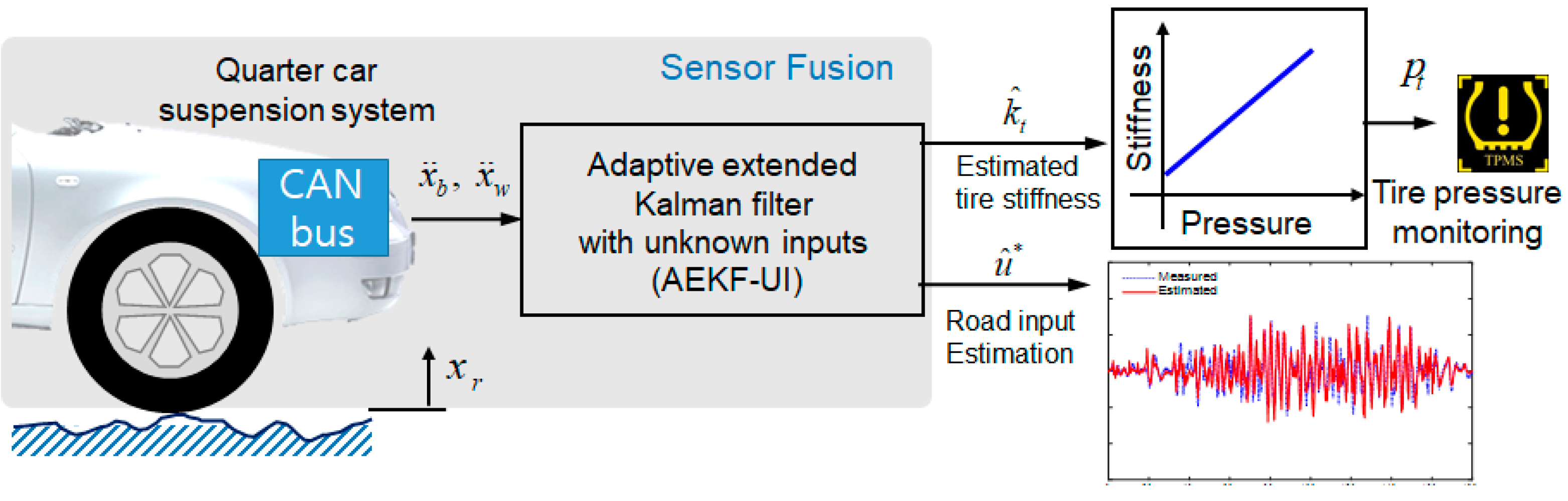
:1. Introduction
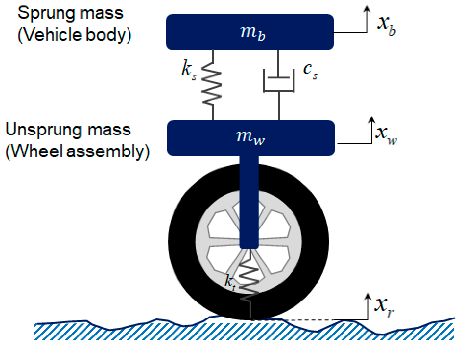
2. Quarter-Car Suspension System
2.1. State-Space Model of Quarter-Car Suspension Systems
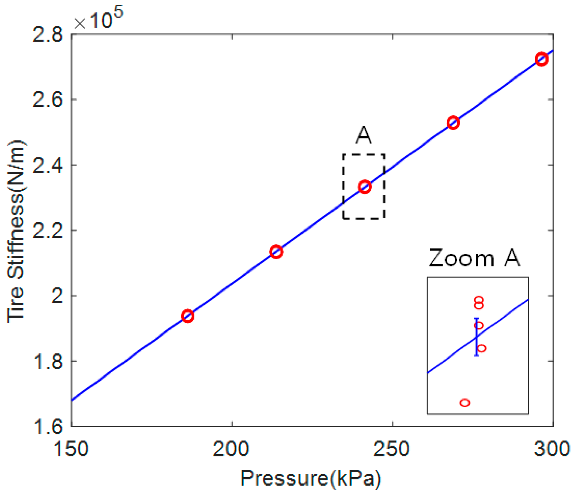
2.2. Relationship between Tire Stiffness and Inflation Pressure
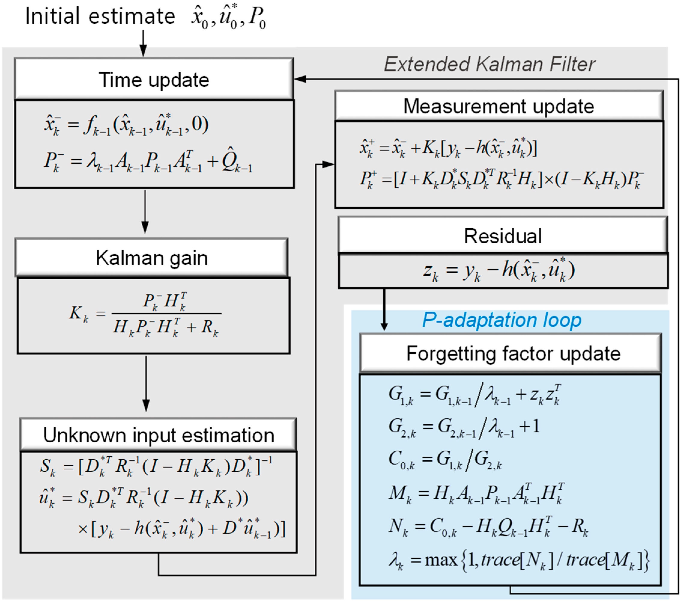
3. Adaptive Extended Kalman Filter with Unknown Input Estimation
3.1. Overview of EKF Algorithm with Unknown Input Estimation
- Initialization of the filter at k = 0
- Prediction stage
- Unknown input estimation
- Correction stage
3.2. Adaptive Extended Kalman Filter with Unknown Input
3.3. Forgetting Factor Update
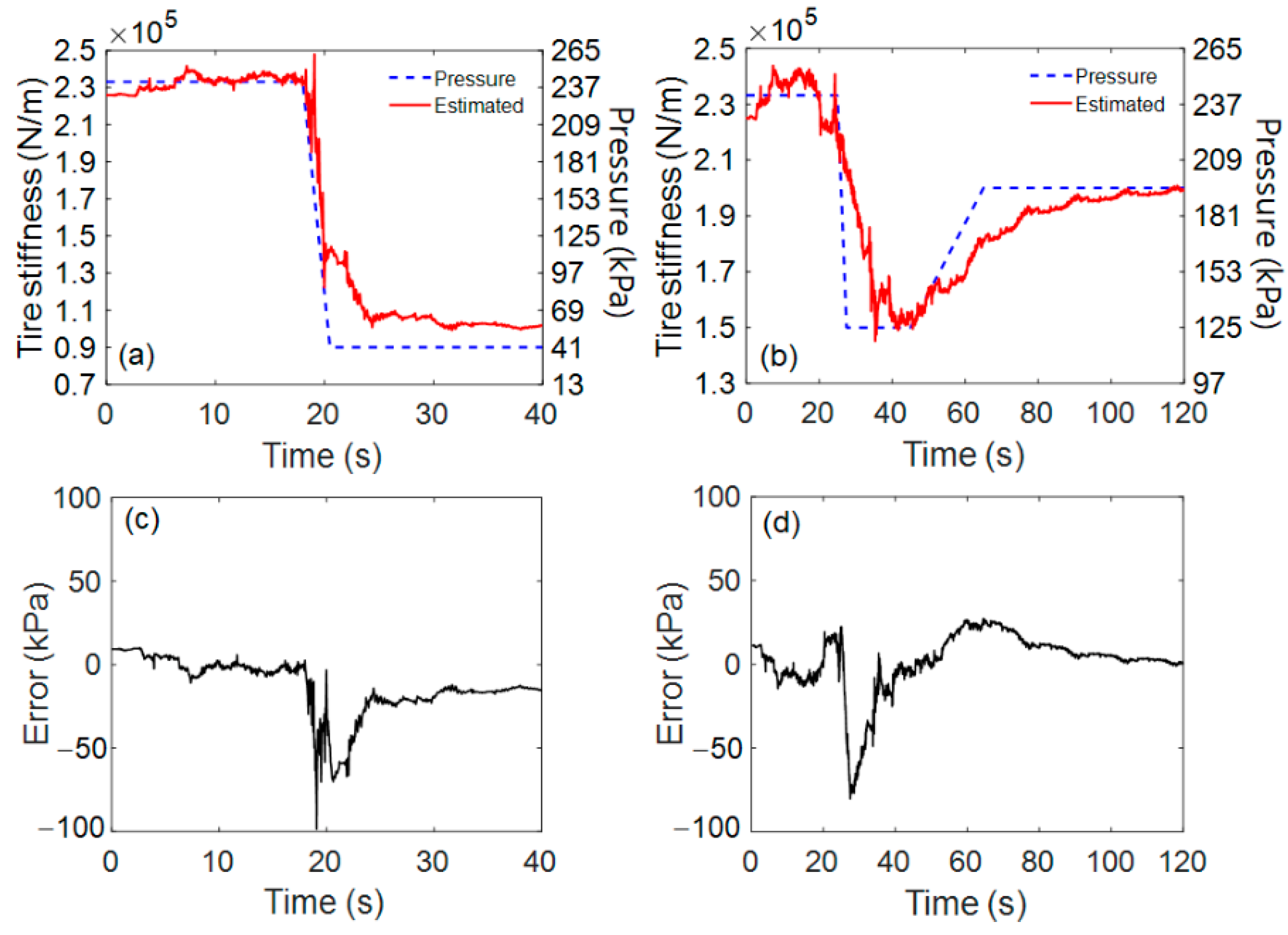
4. Simulation of AKEF-UI Algorithm
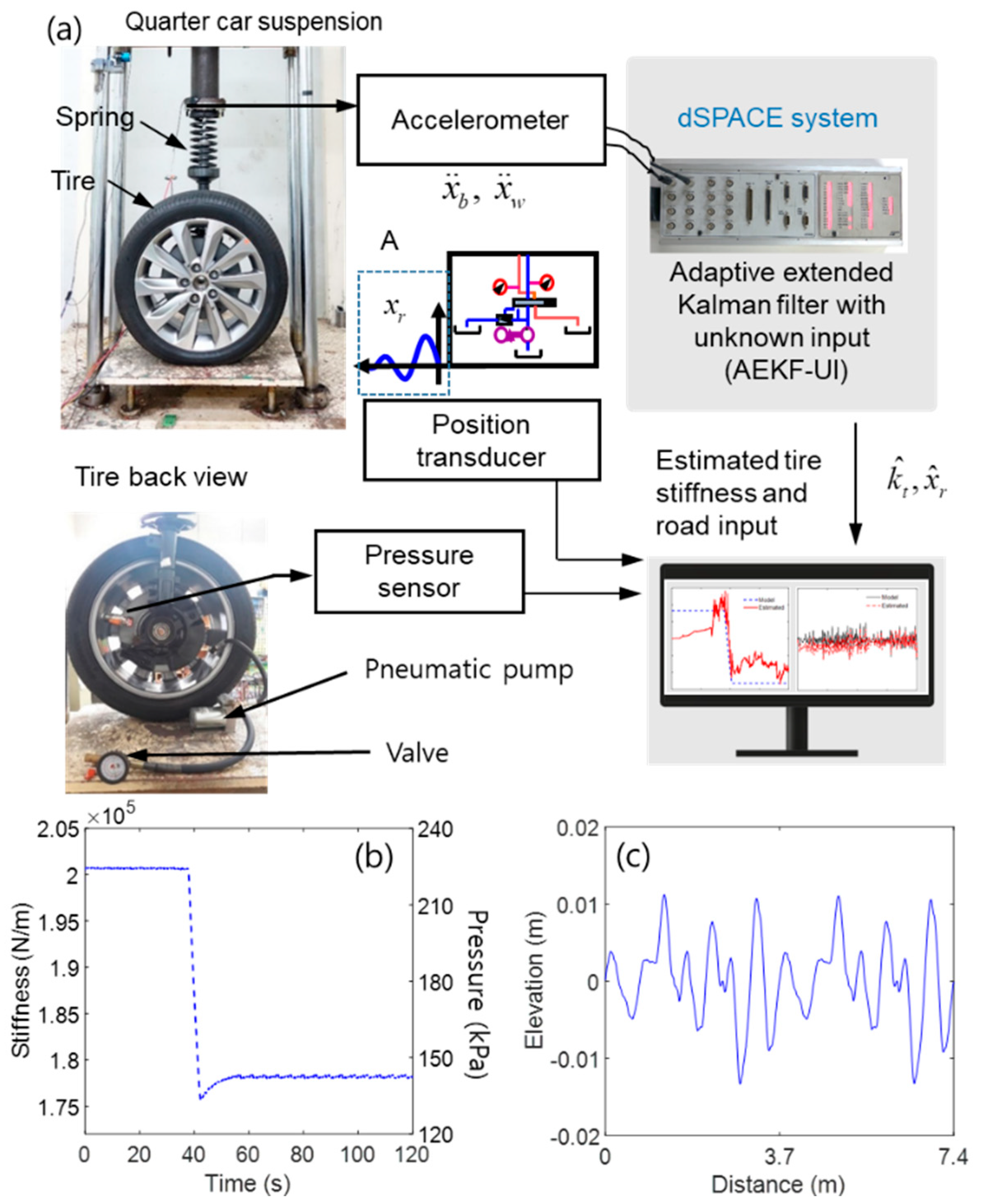
5. Experimental Validation
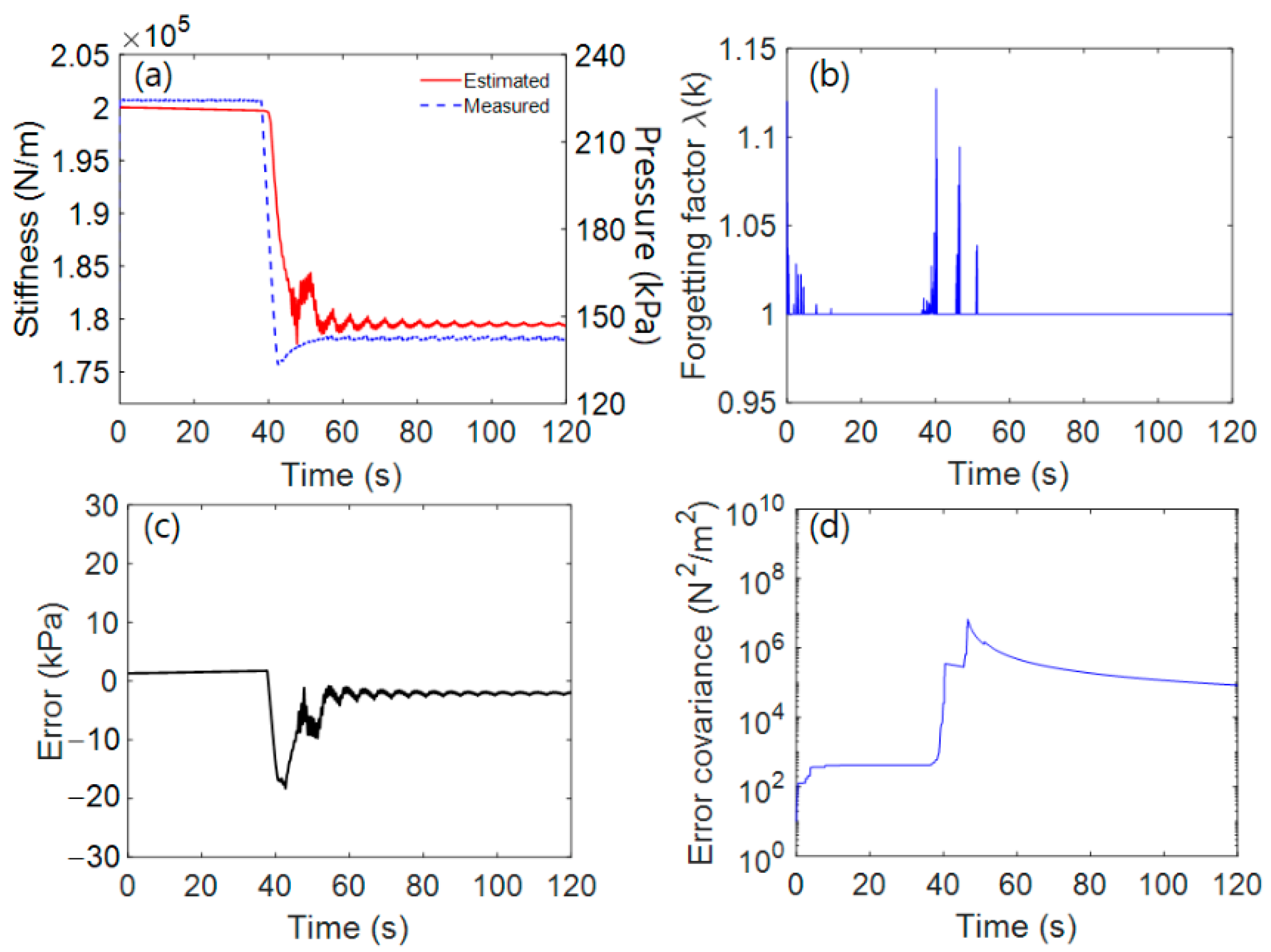
5.1. Proof of Concept Experiment
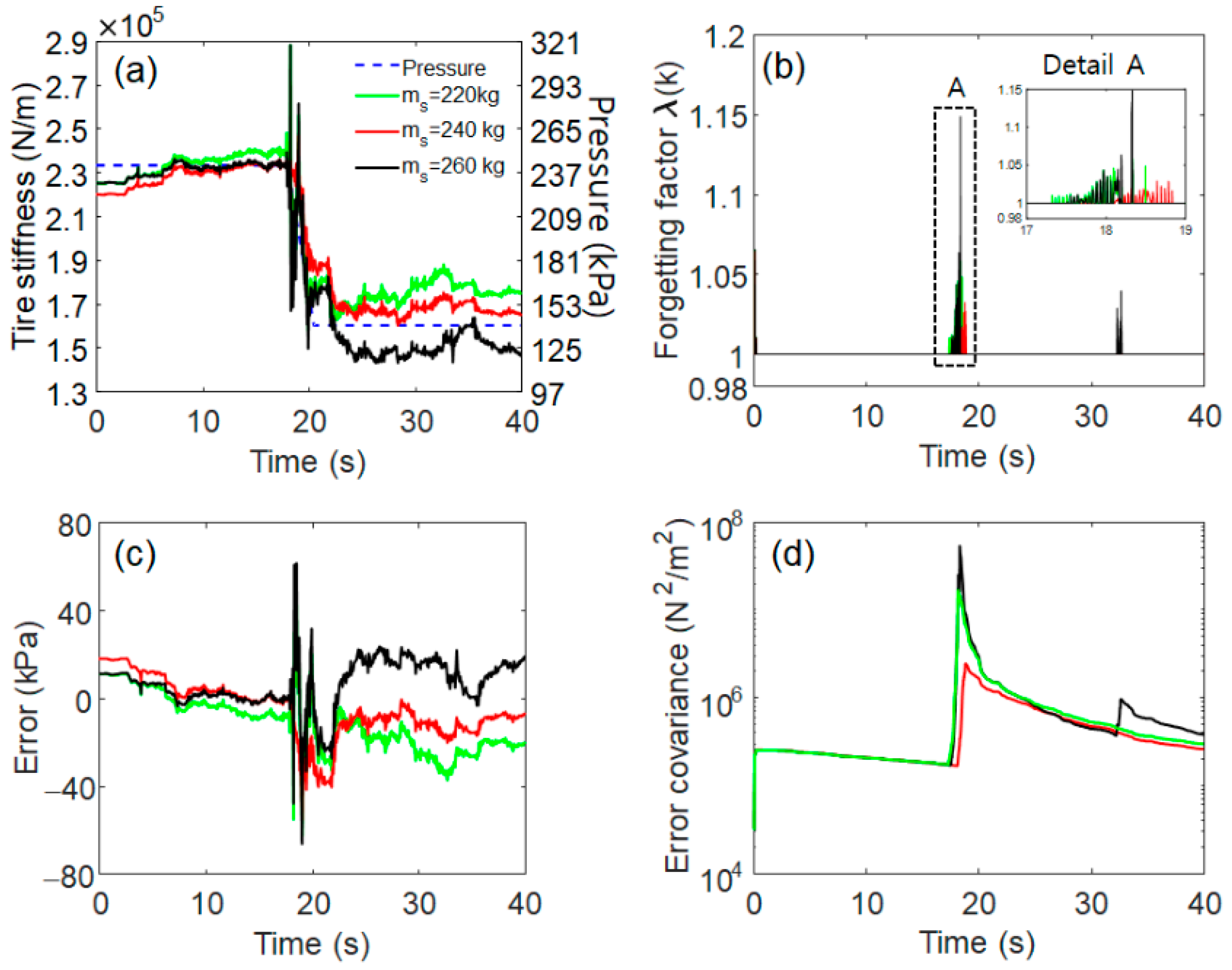
5.2. Robustness Analysis
6. Conclusions
Author Contributions
Funding
Data Availability Statement
Acknowledgments
Conflicts of Interest
References
- Persson, N.; Gustafsson, F.; Drevö, M. Indirect tire pressure monitoring using sensor fusion. SAE Trans. 2002, 1657–1662. [Google Scholar]
- Owende, P.M.; Hartman, A.M.; Ward, S.M.; Gilchrist, M.D.; O’Mahony, M.J. Minimizing distress on flexible pavements using variable tire pressure. J. Transp. Eng. 2001, 127, 254–262. [Google Scholar] [CrossRef]
- Kowalewski, M. Monitoring and managing tire pressure. IEEE Potentials 2004, 23, 8–10. [Google Scholar] [CrossRef]
- Wu, L.; Wang, Y.; Jia, C.; Zhang, C. Battery-less piezoceramics mode energy harvesting for automobile TPMS. In Proceedings of the 2009 IEEE 8th International Conference on ASIC, Changsha, China, 20–23 October 2009; pp. 1205–1208. [Google Scholar]
- Roundy, S. Energy harvesting for tire pressure monitoring systems: Design considerations. In Proceedings of the Power MEMS+ microMEMS, Sendai, Japan, 9–12 November 2008; pp. 9–12. [Google Scholar]
- Zhao, J.; Su, J.; Zhu, B.; Shan, J. An indirect TPMS algorithm based on tire resonance frequency estimated by AR model. SAE Int. J. Passeng. Cars Mech. Syst. 2016, 9, 99–106. [Google Scholar] [CrossRef]
- Silva, A.; Sánchez, J.R.; Granados, G.E.; Tudon-Martinez, J.C.; Lozoya-Santos, J.d.J. Comparative Analysis in Indirect Tire Pressure Monitoring Systems in Vehicles. IFAC PapersOnLine 2019, 52, 54–59. [Google Scholar] [CrossRef]
- Isermann, R.; Wesemeier, D. Indirect vehicle tire pressure monitoring with wheel and suspension sensors. IFAC Proc. Vol. 2009, 42, 917–922. [Google Scholar] [CrossRef]
- Han, J.; Sun, Y.; Tang, X. Research on tire pressure monitoring system based on the tire longitudinal stiffness. In Proceedings of the 2008 IEEE International Conference on Automation and Logistics, Qingdao, China, 1–3 September 2008; pp. 1648–1652. [Google Scholar]
- Marton, Z.; Fodor, D.; Enisz, K.; Nagy, K. Frequency analysis based tire pressure monitoring. In Proceedings of the 2014 IEEE International Electric Vehicle Conference (IEVC), Florence, Italy, 17–19 December 2014; pp. 1–5. [Google Scholar]
- Kang, S.-W.; Kim, J.-S.; Kim, G.-W. Road roughness estimation based on discrete Kalman filter with unknown input. Veh. Syst. Dyn. 2019, 57, 1530–1544. [Google Scholar] [CrossRef]
- Kutluay, E.; Winner, H. Validation of vehicle dynamics simulation models—A review. Veh. Syst. Dyn. 2014, 52, 186–200. [Google Scholar] [CrossRef]
- Yoon, D.-S.; Kim, G.-W.; Choi, S.-B. Response time of magnetorheological dampers to current inputs in a semi-active suspension system: Modeling, control and sensitivity analysis. Mech. Syst. Signal Process. 2021, 146, 106999. [Google Scholar] [CrossRef]
- Türkay, S.; Akçay, H. A study of random vibration characteristics of the quarter-car model. J. Sound Vib. 2005, 282, 111–124. [Google Scholar] [CrossRef]
- Hurel, J.; Mandow, A.; García-Cerezo, A. Kinematic and dynamic analysis of the McPherson suspension with a planar quarter-car model. Veh. Syst. Dyn. 2013, 51, 1422–1437. [Google Scholar] [CrossRef]
- Maher, D.; Young, P. An insight into linear quarter car model accuracy. Veh. Syst. Dyn. 2011, 49, 463–480. [Google Scholar] [CrossRef]
- Rangegowda, P.H.; Valluru, J.; Patwardhan, S.C.; Mukhopadhyay, S. Simultaneous state and parameter estimation using receding-horizon nonlinear kalman filter. IFAC PapersOnLine 2018, 51, 411–416. [Google Scholar] [CrossRef]
- Ding, X.; Wang, Z.; Zhang, L.; Wang, C. Longitudinal Vehicle Speed Estimation for Four-Wheel-Independently-Actuated Electric Vehicles Based on Multi-Sensor Fusion. IEEE Trans. Veh. Technol. 2020, 69, 12797–12806. [Google Scholar] [CrossRef]
- Wang, C.; Wang, Z.; Zhang, L.; Cao, D.; Dorrell, D.G. A Vehicle Rollover Evaluation System Based on Enabling State and Parameter Estimation. IEEE Trans. Ind. Inform. 2020, 17, 4003–4013. [Google Scholar] [CrossRef]
- Taylor, R.; Bashford, L.; Schrock, M. Methods for measuring vertical tire stiffness. Trans. ASAE 2000, 43, 1415. [Google Scholar] [CrossRef]
- Kalman, R.E. A new approach to linear filtering and prediction problems. J. Basic Eng. 1960, 82, 35–54. [Google Scholar] [CrossRef] [Green Version]
- Gelb, A. Nonlinear Estimation. In Applied Optimal Estimation, 6th ed; MIT Press: Cambridge, MA, USA, 1974; pp. 182–199. [Google Scholar]
- Yang, J.N.; Lin, S.; Huang, H.; Zhou, L. An adaptive extended Kalman filter for structural damage identification. Struct. Control Health Monit. Off. J. Int. Assoc. Struct. Control Monit. Eur. Assoc. Control Struct. 2006, 13, 849–867. [Google Scholar] [CrossRef]
- Xia, Q.; Rao, M.; Ying, Y.; Shen, X. Adaptive fading Kalman filter with an application. Automatica 1994, 30, 1333–1338. [Google Scholar] [CrossRef]
- Lou, T.-S.; Wang, Z.-H.; Xiao, M.-L.; Fu, H.-M. Multiple adaptive fading Schmidt-Kalman filter for unknown bias. Math. Probl. Eng. 2014, 2014, 623930. [Google Scholar] [CrossRef] [Green Version]
- Lin, J.W.; Betti, R.; Smyth, A.W.; Longman, R.W. On-line identification of non-linear hysteretic structural systems using a variable trace approach. Earthq. Eng. Struct. Dyn. 2001, 30, 1279–1303. [Google Scholar] [CrossRef]
- Hoshiya, M.; Saito, E. Structural identification by extended Kalman filter. J. Eng. Mech. 1984, 110, 1757–1770. [Google Scholar] [CrossRef]
- Yoshida, I. Damage detection using Monte Carlo filter based on non-Gaussian noises. In Proceedings of the 8th International Conference on Structural Safety and Reliability (ICOSSAR 2001), Newport Beach, CA, USA, 17–22 June 2001. [Google Scholar]
- Loh, C.-H.; Lin, C.-Y.; Huang, C.-C. Time domain identification of frames under earthquake loadings. J. Eng. Mech. 2000, 126, 693–703. [Google Scholar] [CrossRef]
- Kim, G.-W.; Kang, S.-W.; Kim, J.-S.; Oh, J.-S. Simultaneous estimation of state and unknown road roughness input for vehicle suspension control system based on discrete Kalman filter. Proc. Inst. Mech. Eng. Part D J. Automob. Eng. 2020, 234, 1610–1622. [Google Scholar] [CrossRef]
- Varshney, D.; Bhushan, M.; Patwardhan, S.C. State and parameter estimation using extended Kitanidis Kalman filter. J. Process Control 2019, 76, 98–111. [Google Scholar] [CrossRef]
- Ge, Q.; Shao, T.; Duan, Z.; Wen, C. Performance analysis of the Kalman filter with mismatched noise covariances. IEEE Trans. Autom. Control 2016, 61, 4014–4019. [Google Scholar] [CrossRef]
- Huang, Z.; Du, P.; Kosterev, D.; Yang, B. Application of extended Kalman filter techniques for dynamic model parameter calibration. In Proceedings of the 2009 IEEE Power & Energy Society General Meeting (IEEE PES 2009), Calgary, AB, Canada, 26–30 July 2009; pp. 1–8. [Google Scholar]
- Huang, C.; Wang, Z.; Zhao, Z.; Wang, L.; Lai, C.S.; Wang, D. Robustness evaluation of extended and unscented Kalman filter for battery state of charge estimation. IEEE Access 2018, 6, 27617–27628. [Google Scholar] [CrossRef]


| Pressure (psi) | Pressure (kPa) | Stiffness (N/m) |
|---|---|---|
| 27 | 186.2 | 193,780 |
| 31 | 213.7 | 213,450 |
| 35 | 241.3 | 233,350 |
| 39 | 268.9 | 252,960 |
| 43 | 296.5 | 272,440 |
| Symbol | Parameters | Value |
|---|---|---|
| Sprung mass | 240.8 kg | |
| Unsprung mass | 56.9 kg | |
| Damping coefficient | 925.8 N·s/m | |
| Suspension spring constant | 29114 N/m |
| Mass (kg) | RMSE | Relative Error to Nominal |
|---|---|---|
| 220 | 17.57 | 35% |
| 240 (nominal) | 12.96 | - |
| 260 | 13.31 | 2.7% |
| Mass (kg) | RMSE | Relative Error to Nominal |
|---|---|---|
| 220 | 3.48 | 9.7% |
| 240 (nominal) | 3.17 | - |
| 260 | 3.12 | 1.5% |
| Variance | RMSE | Relative Error to Nominal |
|---|---|---|
| 0.248 (nominal) | 3.02 | - |
| 0.274 | 2.67 | 11.58% |
| 0.380 | 4.22 | 39% |
Publisher’s Note:: MDPI stays neutral with regard to jurisdictional claims in published maps and institutional affiliations. |
© 2021 by the authors. Licensee MDPI, Basel, Switzerland. This article is an open access article distributed under the terms and conditions of the Creative Commons Attribution (CC BY) license (https://creativecommons.org/licenses/by/4.0/).
Share and Cite
Lee, D.-H.; Yoon, D.-S.; Kim, G.-W. New Indirect Tire Pressure Monitoring System Enabled by Adaptive Extended Kalman Filtering of Vehicle Suspension Systems. Electronics 2021, 10, 1359. https://0-doi-org.brum.beds.ac.uk/10.3390/electronics10111359
Lee D-H, Yoon D-S, Kim G-W. New Indirect Tire Pressure Monitoring System Enabled by Adaptive Extended Kalman Filtering of Vehicle Suspension Systems. Electronics. 2021; 10(11):1359. https://0-doi-org.brum.beds.ac.uk/10.3390/electronics10111359
Chicago/Turabian StyleLee, Dong-Hoon, Dal-Seong Yoon, and Gi-Woo Kim. 2021. "New Indirect Tire Pressure Monitoring System Enabled by Adaptive Extended Kalman Filtering of Vehicle Suspension Systems" Electronics 10, no. 11: 1359. https://0-doi-org.brum.beds.ac.uk/10.3390/electronics10111359