Adaptive Data Length Method for GPS Signal Acquisition in Weak to Strong Fading Conditions

Abstract

Satellite-based navigation is an essential part of all the technology-dependent applications, such as road transport, cell phones, the medical field, aviation or the shipping industry, etc. The performance of the navigation systems depends upon how quickly they can acquire and process the received signals for positioning solutions. However, in dense urban or indoor environments, signal acquisition can be a challenging task due to fading as a result of multipath and/or interference. This paper presents post-processing acquisition results on Global Positioning System (GPS) signals to study the relationship between data lengths used for signal acquisition and the achieved signal power using a Fast Fourier Transform (FFT)-based circular correlation method. Based on this study, the detection performance of the FFT-based method has also been analyzed by intentionally degrading the signal power levels. A new Adaptive Data length (ADL) method for acquisition has been proposed in this paper, which can be used for speeding up the acquisition process and uses adaptive data lengths rather than fixed data lengths. The ADL method works by estimating the threshold level based on the noise present in the signal and then comparing it with the signal power levels. Less difference between the threshold level and signal power level means less data length will be used while more difference means that more data length will be used for acquisition. The proposed algorithm can be used in commercially available receivers for adopting to an adaptive acquisition process for increased efficiency.

1. Introduction

A large number of the world population lives in urban areas due to increased availability of facilities and ease of access to resources. It is thus necessary to make urban life more sustainable, livable and efficient whilst ensuring safety, security and health. An accurate and reliable positioning service in urban areas by satellite-based navigation systems is essentially important for hundreds of civilian and military applications [1,2,3,4,5,6,7]. At present, there are four independent Global Navigation Satellite Systems (GNSS), including American GPS, Russian GLONASS, European Galileo and Chinese BeiDou Navigation System, providing an easy, efficient and cost-effective way to determine the location, time, and velocity anywhere around the globe [8,9,10]. However, the availability and accuracy of these systems are prone to several atmospheric and environmental conditions such as multipath (MP), interference, electron density irregularities in Earth’s atmosphere, tropospheric delay, and satellite geometry, etc. [11,12,13,14,15,16,17,18,19]. Specifically, in dense urban environments, satellite signals are mainly impaired by strong fading due to multipath and shadowing affecting the accuracy, availability, and continuity of the available navigation systems [20]. The complexity and limitations of satellite signal reception in urban environments are shown in Figure 1. In such environments, the satellite signals are reflected, scattered, fluctuated (i.e., amplitude and phase) and sometimes completely blocked by roofs and walls of highrise buildings, foliages, flyover bridges and complex road scenarios, making the signal acquisition a challenging task [3,21,22].

Out of all the available navigation systems, i.e., GPS, GLONASS, Galileo and BeiDou [8,9,10], the GPS is the oldest and most commonly used system due to its widespread availability for commercial and civilian purposes [24,25,26]. The GPS satellites revolve around the Earth at an altitude of 20,200 km and continuously broadcast navigation signals in the L-band, which are used by the receiver for position estimation [27,28]. The GPS satellite signals are actually bi-phase modulated by a set of distinct orthogonal codes known as the pseudo-random noise (PRN) codes. The two commonly used codes by GPS at $L1$ and $L2$ frequencies are the civilian or Coarse Acquisition ($C/A$) code and the precise code or P code, which is intended for military users [27,29]. A simplified form of the GPS signal structure is given in Figure 2, showing the process of how the navigation message is modulated by the $C/A$ and P codes at the $L1$ and $L2$ frequency bands, respectively.

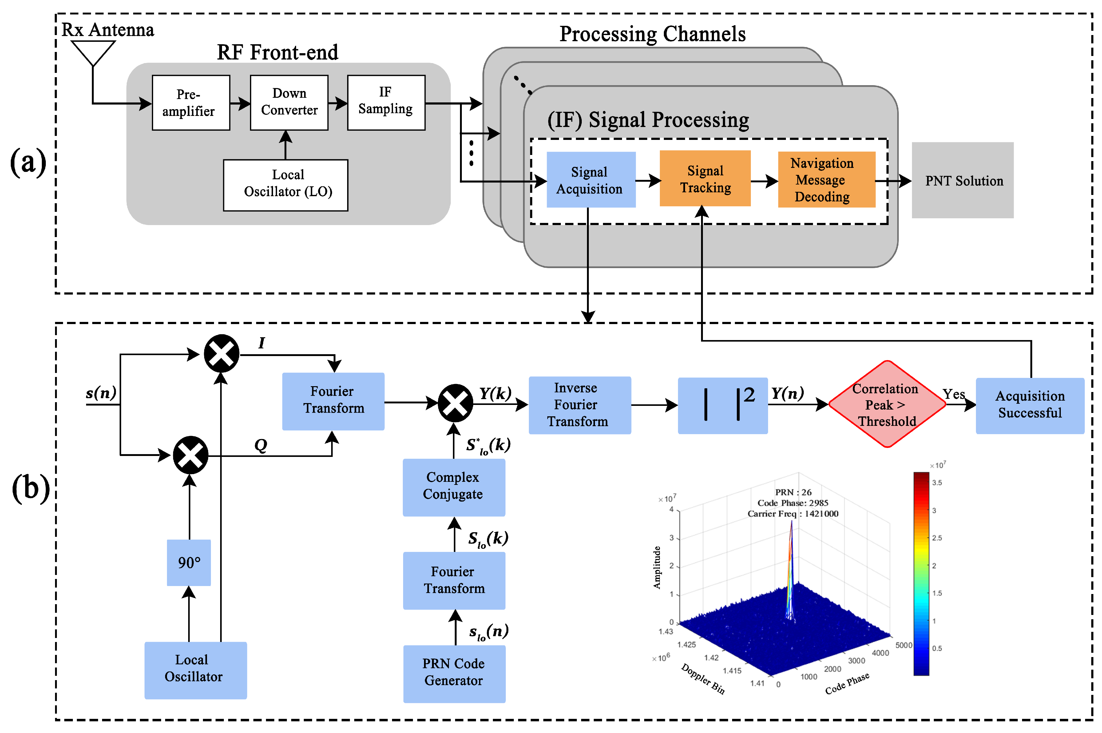
A conventional GPS receiver consists of a Radio Frequency (RF) front-end device that down-converts the received signal into an intermediate frequency (IF) signal, a processing stage where the signal is acquired, tracked and measurements are generated and a Positioning, Navigation and Timing (PNT) solution. The block diagram of a GPS receiver is shown in Figure 3. Once the GPS signal is down-converted by the RF front-end device, the acquisition starts by correlating the incoming received signal with the locally generated replica of the PRN code. The acquisition is declared successful if the correlation peak crosses a threshold level [31,32,33]. In strong signal conditions (i.e., high carrier-to-noise ratio (CNR)), a conventional/commercial receiver works fine but signal acquisition becomes difficult when the CNR of the received signal drops below 35 dB-Hz. A CNR level of 40 dB-Hz and above reflects a strong signal for acquisition and positioning solutions. This can be seen in Figure 4, in which we have shown the lock status of a satellite signal of one of the commercially available high accuracy GNSS receivers, i.e., Septentrio PolaRx5s GPS receiver, deployed in our GNSS and Space Weather Lab, Department of Electrical Engineering, Sukkur IBA University, Pakistan. The results shown in Figure 4 are collected in an environment where the receiver was blocked by a building structure leading to Non-Line-of-Sight (NLOS) signal reception.

Figure 4a shows the received signal CNR, Figure 4b shows the normalized signal strength also known as the signal intensity fluctuations and Figure 4c represents the loss of signal lock by the receiver due to fading or drop in CNR. From 7.5 h to 8.8 h and 10.7 h to 11.5 h, the receiver is continuously losing lock as the CNR level dropped below 35 dB-Hz, leading to large fluctuations in the signal strength. The receiver was able to hold lock only when the CNR rises above 40 dB-Hz, as can be seen in Figure 4c from 8.8 h to 10.7 h, having negligible fluctuations in signal power.

Based on the detailed analysis of real-time GPS signal acquisition using a high-precision, professional-grade GNSS receiver as given in Figure 4, it is obvious that satellite signal acquisition becomes a very challenging task in degraded/obstructed environments. In such environmental contexts, the rapid fluctuations or deep fades in the signal strength due to multipath or NLOS reception can lead to frequent loss of lock events and service interruptions [10]. Although there is substantial research in optimizing the acquisition performance of a GPS receiver, most of the previous work is focused on reducing the computational complexity using fixed data lengths with little or no consideration to severity of signal impairment [34,35,36]. Furthermore, in the case of weak signals, a useful strategy proposed by many researchers [37,38,39,40,41] is to use increased data lengths for acquisition, but this leads to more computational load, leading to long acquisition times, and all the GPS receivers use the same data lengths for strong signals as well, which puts extra burden on the receiver.

In this connection, this paper presents a comprehensive study of fading on GPS signals by using a Fast Fourier Transform (FFT)-based circular correlation method. For this purpose, the GPS signal was intentionally degraded by adding noise through post-processing, and then acquisition was performed to analyze the detection performance in the case of weak to strong fading conditions. Then, in order to solve the problem of fixed data lengths used for weak and strong signal fading, a new adaptive data length-based algorithm is proposed in this paper. The algorithm uses minimum data length of 1 ms for acquisition, and then based, on the difference between the signal power and the threshold level, a decision is made to increase the data length. The proposed algorithm can be quite helpful in adaptive receiver designs, which can reduce a great amount of processing power in terms of the number of computations by avoiding fixed data lengths for acquisition in a receiver and can be incorporated in GPS receivers without any hardware modifications. The proposed algorithm can be implemented using any acquisition method.

2. Signal Acquisition Methodology

The acquisition is the process of generating a local copy of a GPS signal and then correlating it with the incoming received signal to extract the navigation data. The mathematical model of a GPS $L1$ signal [29,42] can be given as

$$S_{L1}\left(t\right)=A_{c}C\left(t\right)D\left(t\right)cos\left(2\pi (f_{L1}+f_d)t\right)+A_{p}P\left(t\right)D\left(t\right)sin\left(2\pi (f_{L1}+f_d)t\right)$$

(1)

where,

• $A_c$: is the amplitude of the C/A code
• $C\left(t\right)$: is the C/A code of the satellite
• $D\left(t\right)$: is the navigation data bits having values $\pm 1$
• $f_{L1}$: is the $L1$ carrier frequency
• $f_d$: is the Doppler shift
• $A_p$: is the amplitude precise code or $P-code$
• $P\left(t\right)$: is the precise code or $P-code$

In case the received signal is affected by fading due to multipath and interference, (1) can be re-written as

$$S_{L1}\left(t\right)=\left(m{A}_c\right)C\left(t\right)D\left(t\right)cos\left(2\pi (f_{L1}+f_d)t\right)+\left(m{A}_p\right)P\left(t\right)D\left(t\right)sin\left(2\pi (f_{L1}+f_d)t\right)$$

(2)

where m is the fading coefficient. As shown in Figure 3a, the RF front end process down-convert the received GPS signal to an intermediate frequency ($f_{IF}$) signal by mixing it with the local oscillator. The $IF$ signal, $S_{IF}$, can be modeled as

$$S_{IF}\left(t\right)=\left(m{A}_c\right)C\left(t\right)D\left(t\right)cos\left(2\pi (f_{IF}+f_d)t\right)+\left(m{A}_p\right)P\left(t\right)D\left(t\right)sin\left(2\pi (f_{IF}+f_d)t\right)$$

(3)

The down-converted signal is then sampled and digitized for further processing. This processing includes acquisition, tracking, navigation data extraction and then position estimation (PNT Solution). The first thing to perform on the incoming signal is the acquisition process, which is shown in Figure 3b. The sampled $IF$ signal at the acquisition block can be given as

$$s\left(n\right)=\left(m{A}_c\right)C\left(n\right)D\left(n\right)cos\left(2\pi (f_{IF}+f_d)n{T}_s\right)+e\left(n\right)$$

(4)

where $T_s$ is the sampling interval ($T_s=1/f_s$), and $e\left(n\right)$ is the noise in the signal from all sources. Acquisition is then performed on the signal $s\left(n\right)$. Figure 3b explains the complete correlation process in acquisition. The sampled IF signal, $s\left(n\right)$ is first mixed with the local oscillator signal to generate the in-phase (I) and quadrature (Q) signals. The two signals are then added together and Fourier transform is performed, which is then multiplied with the Fourier transform of the locally generated $C/A$ code of a particular satellite, which is also referred to as the locally generated signal. The signal after the multiplication process represented by $Y\left(k\right)$ is then passed through the inverse Fourier transform block to finally yield the signal $y\left(n\right)$, which completes the correlation process. The acquisition is a 2-D process, which finds the carrier frequency and beginning of the $C/A$ code of the satellite [27,43]. Mathematically, the complete acquisition process between the received signal, $s\left(m\right)$, and the local replica of that signal, $s_{lo}\left(m\right)$, in time domain can be given as

$$y\left(n\right)=\sum _{m=0}^{N-1}s\left(m\right)s_{lo}(m-n)$$

(5)

Acquisition is declared only if any of the peak crosses a pre-defined threshold level. There exists several methods used for GPS signal acquisition such as the FFT-based circular correlation method, delay and multiply method, block-repetition method, double block zero padding method, data folding method and the serial search method [44,45]. The overall acquisition strategy used by all the acquisition methodologies is the same, which is shown in Figure 3b. Most of the acquisition methodologies work on compromising the Signal-to-Noise Ratio (SNR) over speed; however, the FFT-based circular correlation method is the most feasible in case high CNR is required, as mentioned by many researchers [34,35,36,46,47,48], but at the expense of reduced speed. In fact, it has also been reported that the FFT-based circular correlation method is recommended for weak signal acquisition due to its high detection performance. Therefore, this paper also uses this method for acquisition rather than comparing the different acquisition methodologies in order to propose a new GPS receiver design, which could effectively implement the FFT-based circular correlation acquisition with increased speed and efficiency. In Figure 3b, the Fourier transform-based correlation between the received signal and the local signal can be given as

$$Y\left(k\right)=\sum _{n=0}^{N-1}y\left(n\right)W_N^{nk}=\sum _{n=0}^{N-1}\sum _{m=0}^{N-1}s\left(m\right)s_{lo}(m-n)W_N^{nk}$$

(6)

The above equation can also be re-arranged as

$$Y\left(k\right)=\underset{S\left(k\right)}{\underbrace{\sum _{m=0}^{N-1}s\left(n\right)W_N^{nk}}}\underset{S_{lo}^{*}\left(k\right)}{\underbrace{\sum _{n=0}^{N-1}{s}_{lo}(m-n)W_N^{-(m-n)k}}}$$

(7)

where $W_N^{nk}=e^{-j2\pi kn/N}$ is the twiddle factor. Representing the first term by $S\left(k\right)$ and the second term by $S_{lo}^{*}\left(k\right)$, (7) can be re-written as

$$Y\left(k\right)=S\left(k\right)S_{lo}^{*}\left(k\right)$$

(8)

where $S_{lo}^{*}\left(k\right)$ is the complex conjugate of $S_{lo}\left(k\right)$. The signal $Y\left(k\right)$ is the correlator signal. To complete the correlation process and to get the final acquisition result, the inverse Fourier transform of $Y\left(k\right)$ is taken to get $y\left(n\right)$. Once the correlation process is complete, the next step is to find out whether there is any satellite present or not. This can be done by searching for the correlation peak or the highest signal power from the acquisition results given as

$$P_{N,max}=max{\left|y\left(n\right)\right|}_N$$

(9)

If the peak, $P_{N,max}$, crosses the threshold level ($\gamma$), the satellite is said to be present, otherwise the whole process must be kept on repeat for the next block of data. The main thing in this whole process is selecting the threshold ($\gamma$), which is based on the false alarm probability and SNR, and these two can be severely affected by multipath or interference. More fading means that the signal level will be lower than the threshold level and the receiver will be unable to declare acquisition or there can be false acqusition. The SNR in this paper has been estimated by the following equation

$$SNR={\displaystyle \frac{|P_{N,max}{|}^2}{{\sigma }_n^2}}$$

(10)

where ${\sigma }_n^2$ is the noise variance. Equation (10) is also known as the post correlation SNR and is used as a standard way of measuring the received signal power. In case the signal is weak, the only way to increase the signal power is to increase the data length for acquisition and for this purpose, coherent and non-coherent integration approaches are used. However, coherent integration is more useful in weak signal conditions but at the expense of an increased number of computations [37,49]. In this paper, we will be using non-coherent integration for signal acquisition.

3. Methodology and Experimental Setup

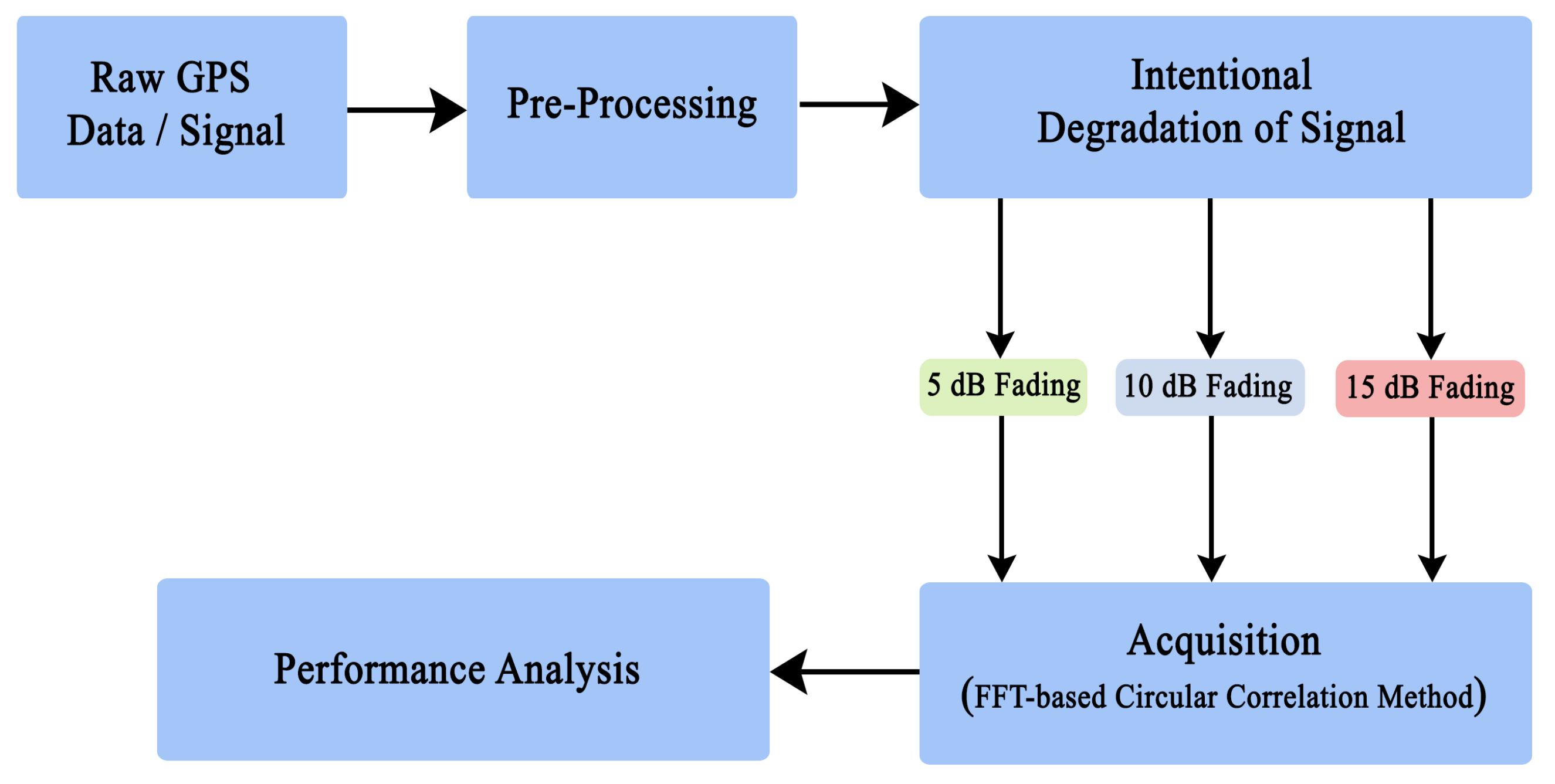
The aim of this paper is twofold; (1) to present the comprehensive study of fading effects on the acquisition performance of a GPS receiver by analyzing signal strength, data length, acquisition time and detection probability; (2) a new adaptive data length algorithm (ADL) is proposed for efficient signal acquisition, which adaptively selects the optimal data length by estimating the severity of the fading level. The overall methodology of this study and flowchart of the proposed ADL algorithm are given in Figure 5 and Figure 6, respectively. The whole process starts by acquiring and then processing (i.e., frequency down-conversion and sampling) a raw GPS signal, which is then intentionally degraded by adding noise through post-processing. Three test signals of different fading levels (e.g., 5, 10, 15) are generated, and acquisition using FFT-based circular correlation is performed on each test signal. Finally, a new adaptive data length algorithm is proposed to improve the acquisition performance, and the details, flowchart, and implementation of the proposed ADL algorithm are given in Section 6.

The data used in this paper are the raw GPS signals collected by using the USRP (Universal Software Radio Peripheral) N210 device. The USRP is a general purpose and reconfigurable Software Define Radio (SDR), mostly used in research and academia to prototype and deploy wireless communication systems. It utilizes the combination of host-based processors, FPGAs, and RF front ends to receive, transmit and analyze the real-world signals. The USRP N210 version provides high-bandwidth, high-dynamic range processing capability with modular design, supporting it to operate up to 6 GHz [50]. The radio typically used in N210 operates at wider frequencies ranging from 50 MHz to 2.2 GHz and provides 40 MHz of bandwidth capability. The powerful processing capability of onboard FPGAs is especially beneficial for applications that require processing wide bandwidths of data in real-time. The experimental setup for recording the GPS signal is shown in Figure 7 below. The Septentrio receiver is used for just checking the signal quality in this experiment only.

Collecting raw GPS data using generic SDRs (e.g., USRP) is not an easy task as the GPS signal is already very weak when received at the front-end device. The task is more difficult when the signal is recorded in dense urban environments. Therefore, to mimic the effects of fading due to multipath or interference, the signal was intentionally degraded by adding noise into the signal after reception to lower its SNR. In this paper, the signal is down-converted at a frequency of $1.42$ MHz and sampled at 5 MHz and acquisition is performed on the $C/A$ code only. Since the $C/A$ code is a 1 ms long PRN code with a chip rate of 1.023 MHz, at the given down conversion rate, the received signal will have 5000 data samples in 1 ms of received signal. In this paper, we use 1 ms or 5000 data points simultaneously to refer to 1 ms of data. Acquisition is then performed using the FFT-based correlation method over blocks of 1 ms of data in the $\pm 10$ KHz Doppler frequency range. Acquisition is declared successful only if the signal peak $|P_{N,max}{|}^2>\gamma$. Here, the $\gamma$ depends upon the probability of a false alarm and the post-correlation SNR, whose complete description is given in Section 5. If the acquisition is not successful using 1 ms of data, then a further 1 ms of data is used through non-coherent integration. Since the GPS navigation data length is 20 ms, to avoid bit transition, which occurs every 20 ms, the non-coherent integration is restricted to 20 ms.

4. Fading Effects on Acquisition and Signal Power Levels

As discussed earlier, the satellites in GPS are represented by unique PRN codes assigned to them, i.e., satellite 1 is denoted by PRN 1, satellite 2 by PRN 2, and so on. Acquisition is then performed on the collected data and the acquisition results of one of the acquired satellite, i.e., PRN 26 are shown in Figure 8. The graph compares the SNR versus the data length (integration time) used for acquisition. The acquisition is performed on a total of 20 ms of data starting from 1 ms. The experiment is divided into three cases. A signal with 5 dB fading is shown by a green line, the 10 dB fading case is shown by a blue line and the 15 dB fading case is shown by the red line. The red circles in Figure 8 are the points where acquisition was declared once the signal was found for the 5 dB, 10 dB and 15 dB fading cases.

It can be seen in Figure 8 that the 5 dB faded signal used only 1 ms of data for acquisition, the 10 dB faded signal used 4 ms of data, while the 15 dB case took 7 ms of data for acquisition. It must be noted that 1 ms of data contains 5000 samples; thus, in order to acquire a GPS signal with 15 dB of fading, the receiver had to use 45,000 samples for processing, which requires a lot of computational power. All the modern receivers use the maximum length of data for acquisition, which may not be required in case of less fading, as can be seen in the 5 dB fading case, which used only 1 ms of data for successful acquisition. Therefore, a strategy must be developed that can use varying data lengths for acquisition in the case of weak or strong fading levels. 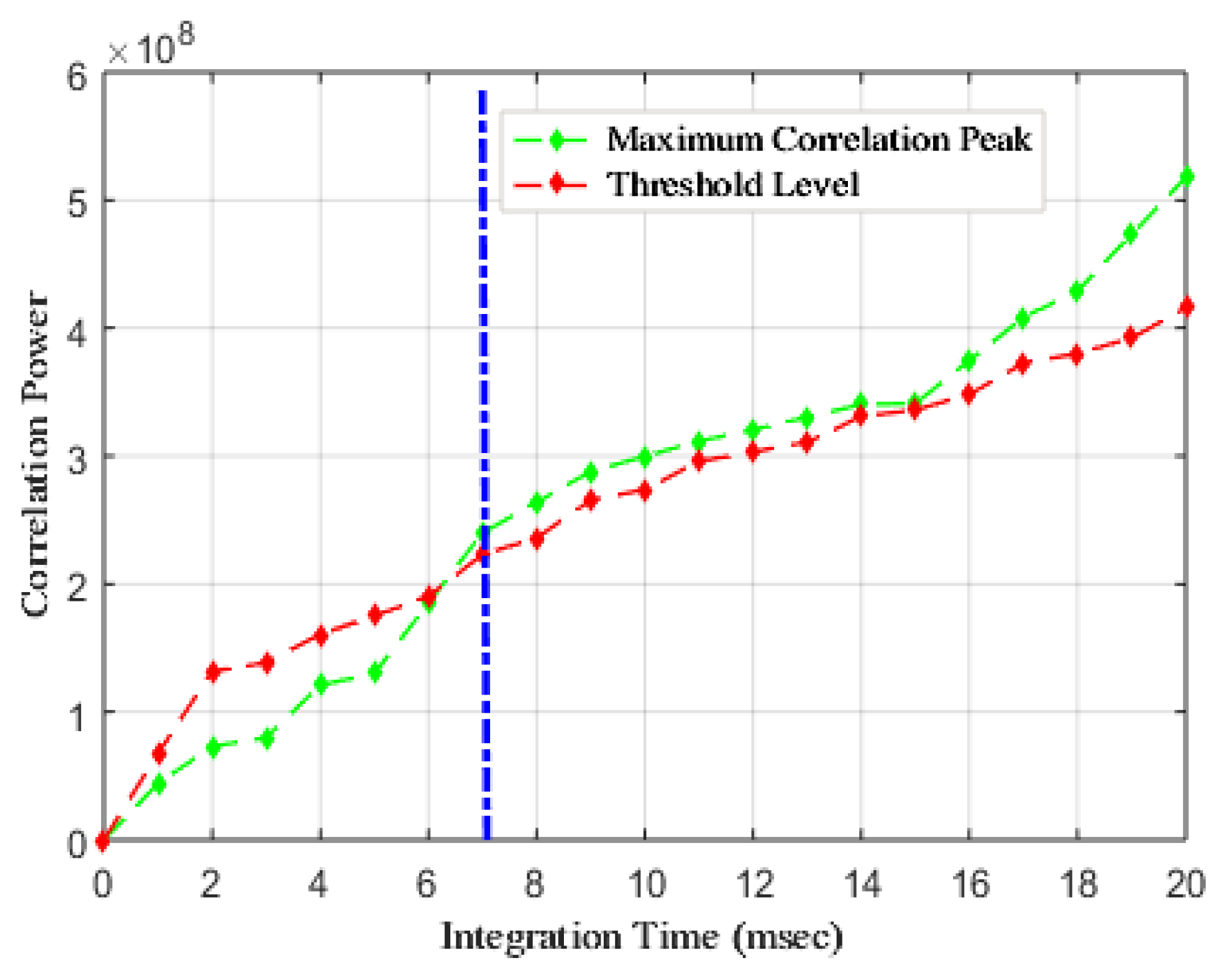The results in Figure 8 are then further elaborated individually in Figure 9, Figure 10 and Figure 11 for PRN 26. These figures developed the relationship between the data length (integration time), correlation power and the threshold level used for acquiring the GPS signal. 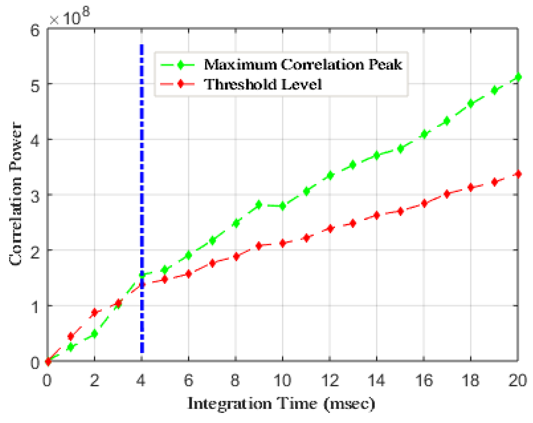Figure 9 represents the acquisition result of the 5 dB fading case. The green line in Figure 9 shows the maximum signal/correlation power plotted against the data length used for acquisition. The red line is the threshold estimated for that particular length of data, whereas the vertical blue line is the point where the signal power (green line) has crossed the threshold level (red line), which is 1 ms in the case of 5 dB fading.

The threshold used is adaptive and based on overall noise present in the signal. The description of how the threshold is estimated is given in the next section. In Figure 9, although only 1 ms of data was used for successful acquisition, if the same process is repeated for the next cycle of data, then it may be possible that the acquisition is not successful, as the noise may increase in the signal due to less difference between the correlation power and threshold level. The results of integration time versus the correlation power for the 10 and 15 dB fading cases are shown in Figure 10 and Figure 11, respectively. In both cases, as a result of more noise, a longer integration time has been taken up by the receiver for acquisition. In Figure 10, it can be seen that the correlation power was below the threshold level up until 3 ms of data. The signal correlation power crossed the threshold level at 4 ms of data and then remained higher than the threshold level. Similarly, in Figure 11, for the 15 dB fading case, the correlation power level crossed the threshold level at the 7 ms of data. These results show that the fading in the signal, whether it be due to multipath or interference, can severely affect the receiver capability of locking onto the satellites. More fading means that more time will be required by the receiver for acquisition, which can lead to reduced efficiency in critical applications.

Figure 12, Figure 13 and Figure 14 show the actual acquisition results of PRN 26 as acquired by the receiver for the 5, 10 and 15 fading cases, respectively. The results show acquisition in each case for up to 8 ms of data, as the signal was acquired in all the cases using this data length. The main objective of showing the acquisition results is to show the peak signal correlation power and level of noise in the signal. It can be seen that as the noise level goes higher as well as the threshold level due to its adaptive nature, as it depends on the noise present in the signal. Choosing a higher data length leads to increased signal power but at the expense of more computational and processing power.

5. Detection Performance

In order to analyze the efficiency of a GPS receiver, the detection performance plays an important part. The detection performance not only depends upon the false alarm detection but also the noise present in the signal. Let us assume that the correlation between the incoming GPS signal and the local signal is represented by $\widehat{S}\left(k\right)$ then from (8), the output of a correlator in the presence of noise, $\widehat{n}\left(k\right)$, can be represented as

$$Y\left(k\right)=\widehat{S}\left(k\right)+\widehat{n}\left(k\right)$$

(11)

Based on the noise level, there exist two possibilities when acquisition is performed on the incoming GPS signal by the receiver, i.e., signal is not detected, and the signal is detected. In case the signal is present but not detected by the receiver, the Probability Density Function (PDF) of the noise envelope, z, can be given as

$$p\left(z\right)=z/{\sigma }_n^2{e}^{-({\gamma }^2/2{\sigma }_n^2)}$$

(12)

where $\gamma$ is the threshold and ${\sigma }_n^2$ is the noise variance. (12) can also be used to find out the probability of a false alarm. We assume that there is no signal present but any one of the noise components crosses the threshold $\gamma$, which means that there is a false detection. In this case, the probability of false alarm can be found as

$$P_{fa}={\int }_{\gamma }^{\infty }p\left(z\right)dz=e^{-({\gamma }^2/2{\sigma }_n^2)}$$

(13)

Re-arrangement of (13) can be used to find out the threshold level as

$$\gamma =\sqrt{-2{\sigma }_n^{2}ln\left(P_{fa}\right)}$$

(14)

Equation (14) is the threshold that we have used in our proposed acquisition methodology for selecting the data lengths for acquisition. The threshold level depends on noise given by its variance ${\sigma }_n^2$. More noise means a higher threshold level, and therefore, it is adaptive in nature. In case the signal with an amplitude of A is also present along with the noise, then the PDF of the noise function [51] can be given as

$$p\left(z\right)={\displaystyle \frac{z}{{\sigma }_n^2}}exp\left(-{\displaystyle \frac{{\gamma }^2+A^2}{2{\sigma }_n^2}}\right)I_o\left({\displaystyle \frac{zA}{2{\sigma }_n^2}}\right)$$

(15)

where $I_o\left(X\right)$ is the zero order modified Bessel function. From (15), the probability of detection $\left(P_d\right)$ can be found as

$$P_d={\int }_{\gamma }^{\infty }{\displaystyle \frac{z}{{\sigma }_n^2}}exp(-{\displaystyle \frac{{\gamma }^2+A^2}{2{\sigma }_n^2}})I_o\left({\displaystyle \frac{zA}{2{\sigma }_n^2}}\right)dz$$

(16)

Using series approximation [52], the detection probability after the integration is

$$P_d=0.5\left[1-erf({\displaystyle \frac{\gamma -A}{\sqrt{2{\sigma }_n^2}}})\right]+\left\{\frac{exp\left[-{(\gamma -A)}^2/{\sigma }_n^2\right]}{2\sqrt{2\pi }(A/\sqrt{{\sigma }_n^2)}}\right\}\times \left\{1-\frac{\gamma -A}{4A}+{\displaystyle \frac{1+\left[{(\gamma -A)}^2/{\sigma }_n^2\right]}{8A/{\sigma }_n^2}}\right\}$$

(17)

The detection performance of 5 dB, 10 dB and 15 dB fading cases is shown in Figure 15, where the detection probability is estimated in each case with respect to integration time used for acquisition. The results in Figure 15 show that the detection probability deceases with increased fading level. For an efficient receiver, a detection performance of almost $90\%$ is desired. However, in the case of 15 dB fading, as shown by the red dotted line, a 90% detection performance can only be achieved when more than 10 ms of data will be used for acquisition. This is not practical in most of the receivers due to high computational cost. This further shows that in the case of strong fading levels, the use of more data length may not give the desired performance.

6. Adaptive Data Length (ADL) Method for Efficient Signal Acquisition

Based on the above acquisition results and after analyzing the receiver performance in weak to strong fading conditions, we concluded that the acquisition performance of a GPS/GNSS receiver is greatly influenced by the characteristics of signal strength. Due to poor signal strength and deep fades, the signal acquisition becomes a very challenging task. Most of the previous studies show that larger data accumulation can be effective in the acquisition of a weak/impaired GPS signal [37,46,49]. However, using fixed long data lengths for acquisition may not be an optimal solution in all cases. For instance, in the case of a weak signal fading, although a higher data length can increase the SNR of the signal, it may not be desired due to increased acquisition time. 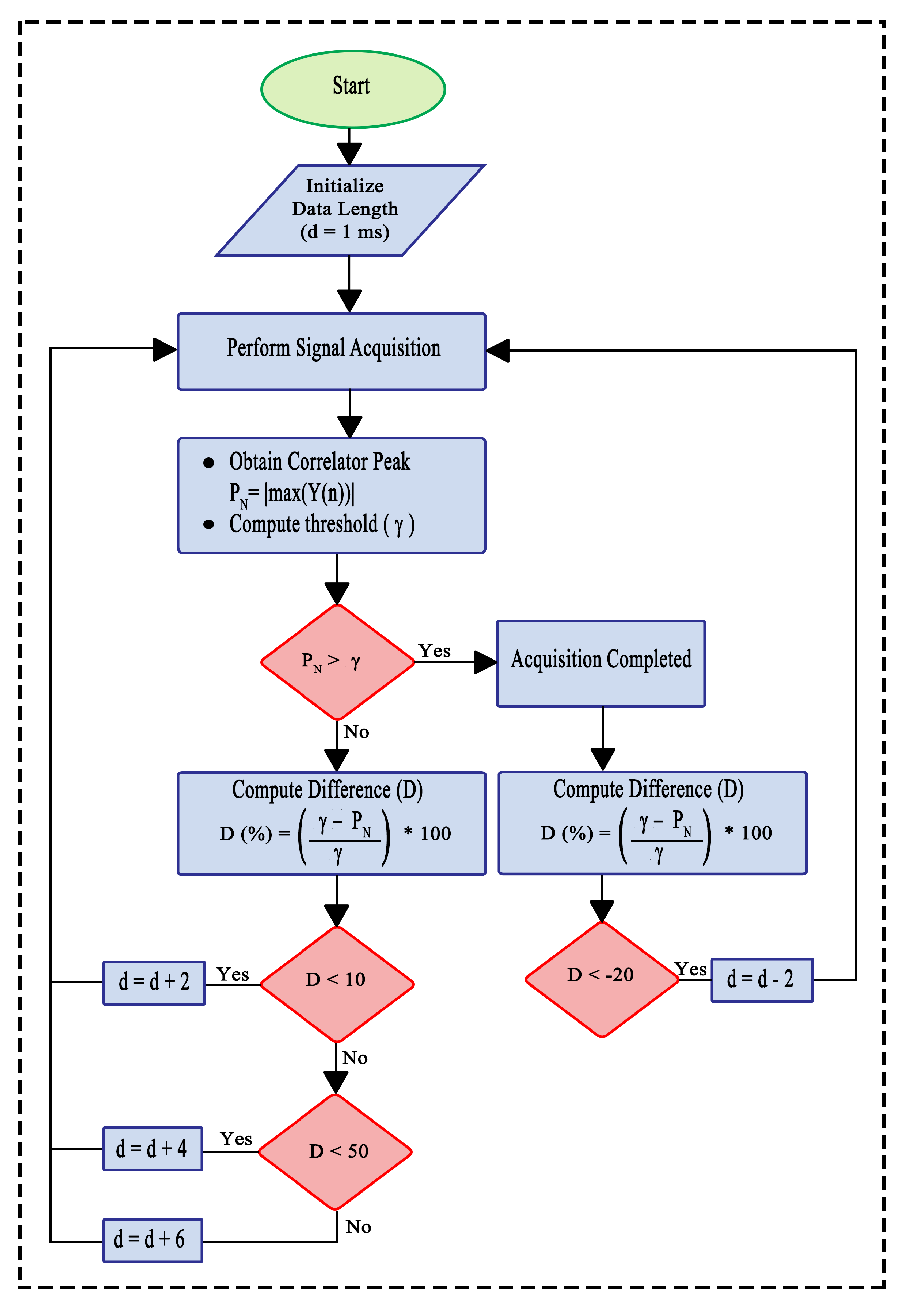Most of the modern available GPS receivers use fixed data lengths for acquisition based on the worst available scenario and, therefore, end up using the same long data lengths for clear line-of-sight scenarios where it is not required [53,54]. However, the service disruption to GPS occurs only when the user moves to a very densely populated area covered by tall buildings, trees or bridges. Considering all the scenarios and the receiver performance scales, a new Adaptive Data Length (ADL) algorithm has been proposed for efficient signal acquisition. The proposed acquisition method estimates the severity of signal impairment by computing the difference ($D(\%)$) between signal peak power ($P_N$) and threshold level $\left(\gamma \right)$ to select the optimal data length for efficient signal acquisition. The flow chart of the proposed ADL method is shown in Figure 6. The method works by initially starting with a standard data length of 1 ms for acquisition. The signal peak, $P_N$, is then compared with the threshold level, $\gamma$. If the $P_N>\gamma$, acquisition will be declared; otherwise, the difference between the peak signal power $P_N$ and $\gamma$ is computed. The higher value of $D(\%)$ indicates the strong fading level, whereas the small value of $D(\%)$ is an indication of a lower fading level. The ADL decides the data length based on a value of $D(\%)$, i.e., if at the initial stage, the difference D is less than $10\%$, then only 2 ms of additional data will be used for acquisition of the previously used data length. However, in case the difference is greater than $10\%$, then another check of $50\%$ is introduced. If the difference, D, is less than $50\%$, then 4 ms of additional data length will be used for acquisition, and in case D is greater than $50\%$, then the acquisition will add up to 6 ms of extra data length of the previously used data length. This way, a more efficient method of receiver design can be adopted for signal acquisition. The values of $D(\%)$ and additional data lengths used by ADL are selected based on the detailed analysis of acquisition performance under different fading levels, as given in Section 4. The ADL method can be incorporated in a receiver at the acquisition stage for making the acquisition process adaptive.

The proposed ADL method is then validated by performing acquisition on the actual GPS signal using the FFT-based circular correlation technique. The signal used for this purpose is a 15 dB faded signal. The results are shown in

Table 1. Acquisition performed on the 15 dB faded signal using the Adaptive Data Length (ADL) method.

Acquisition Attempt	1st Itr. d (ms)	D (%)	2nd Itr. d (ms)	D (%)	3rd Itr. d (ms)	D (%)	Remarks on Acquisition
01	01	31.4	05	−32 ($P_N>\gamma$)	N/A	N/A	Acquisition declared in 2nd iteration using 5 ms of data
02	01	30.8	05	43.5	09	−85.7 ($P_N>\gamma$)	Acquisition declared in 3rd iteration using 9 ms of data
03	01	27.3	05	−135 ($P_N>\gamma$)	N/A	N/A	Acquisition declared in 2nd iteration using 5 ms of data
04	01	34.0	05	32.1	09	−5.3 ($P_N>\gamma$)	Acquisition declared in 3rd iteration using 9 ms of data
05	01	11.1	05	−35.6 ($P_N>\gamma$)	N/A	N/A	Acquisition declared in 2nd iteration using 5 ms of data
06	01	37.3	05	−36.5 ($P_N>\gamma$)	N/A	N/A	Acquisition declared in 2nd iteration using 5 ms of data
07	01	31.6	05	23.6	09	−47.3 ($P_N>\gamma$)	Acquisition declared in 3rd iteration using 9 ms of data
08	01	28.9	05	−17.8 ($P_N>\gamma$)	N/A	N/A	Acquisition declared in 2nd iteration using 5 ms of data
09	01	39.9	05	9.2	07	−21.0 ($P_N>\gamma$)	Acquisition declared in 3rd iteration using 7 ms of data
10	01	52.6	07	−5.8 ($P_N>\gamma$)	N/A	N/A	Acquisition declared in 2nd iteration using 7 ms of data

, where ten different attempts were made on the signal for acquisition at different times for testing purposes. As mentioned earlier, the noise is random in nature and therefore sometimes a signal that is acquired using 7 ms of data may need only 3 ms or 4 ms of data for acquisition at a further point in time. The acquisition starts as per the flowchart of the algorithm given in Figure 6. In the first attempt in Table 1, the ADL method starts by performing acquisition on 1 ms of data. The reason to start with 1 ms is due to the fact that we also have to consider the weak fading conditions where the signal may be acquired using only 1 ms or 2 ms of data. Larger data lengths are required whenever the user moves into fading conditions having NLOS signal reception, such as dense urban or indoor environments. For 1 ms of data, $P_N<\gamma$, the algorithm moves to the next step to estimate the difference $D(\%)$ between the peak signal power and the threshold power level, which is $31.4\%$ and is greater than $10\%$ but less than $50\%$; thus, the algorithm will move into the second iteration for acquisition by using 4 ms of additional data length. In the second iteration, the total data length used for acquisition is now 5 ms. In the second iteration of the first acquisition attempt, the power level difference is found to be $-32\%$, which shows that the peak signal power has crossed the threshold level, i.e., $P_N>\gamma$. At this point, acquisition will be declared, and the process will stop. Similarly, the second acquisition attempt in the second row of Table 1 uses three iterations and a total of 9 ms of data for acquisition, whereas the third acquisition attempt uses two iterations and 5 ms of data for acquisition. The last acquisition attempt, i.e., 10th acquisition attempt, uses 7 ms of data and two iterations for successful acquisition.

The 15 dB faded signal case used a maximum of two to three iterations for successful acquisition of the GPS signal. The study on the validity of the proposed ADL method is then further extended on a 20 dB faded signal to observe the performance of the ADL method in the case of very weak signals.

Table 2. Acquisition performed on the 20 dB faded signal using the Adaptive Data Length (ADL) method.

Acquisition Attempt	1st Itr. d (ms)	D (%)	2nd Itr. d (ms)	D (%)	3rd Itr. d (ms)	D (%)	4th Itr. d (ms)	D (%)	5th Itr. d (ms)	D (%)	Remarks on Acquisition
01	01	54.9	07	11.2	11	−10.31 ($P_N>\gamma$)	N/A	N/A	N/A	N/A	Acquisition declared in 3rd iteration using 11 ms of data
02	01	57.1	07	52.9	13	31.94	17	−3.78 ($P_N>\gamma$)	N/A	N/A	Acquisition declared in 4th iteration using 17 ms of data
03	01	53.0	07	63.6	13	15.41	17	−14.2 ($P_N>\gamma$)	N/A	N/A	Acquisition declared in 4th iteration using 17 ms of data
04	01	16.2	07	33.9	11	21.02	15	−9.5 ($P_N>\gamma$)	N/A	N/A	Acquisition declared in 4th iteration using 15 ms of data
05	01	64.7	07	29.9	11	15.4	15	20.1	19	−13.3 ($P_N>\gamma$)	Acquisition declared in 5th iteration using 19 ms of data
06	01	46.4	05	53.2	11	49.2	15	28.93	19	34.4	Acquisition not declared in 2nd iteration using 5 ms of data
07	01	66.2	07	45.8	11	52.01	17	7.82	19	−3.7 ($P_N>\gamma$)	Acquisition declared in 5th iteration using 19 ms of data
08	01	63.3	07	28.3	11	27.32	15	−12.36 ($P_N>\gamma$)	N/A	N/A	Acquisition declared in 4th iteration using 15 ms of data
09	01	51.5	05	16.5	11	−2.71 ($P_N>\gamma$)	N/A	N/A	N/A	N/A	Acquisition declared in 3rd iteration using 11 ms of data
10	01	61.8	07	2.64	11	19.53	15	3.6	19	−9.73 ($P_N>\gamma$)	Acquisition declared in 5th iteration using 19 ms of data

shows the acquisition results of the ADL method performed on the 20 dB faded signal. In some cases, it took only 10 ms of data for acquisition, whereas in others, it took 19 ms of data for acquisition. In the first acquisition attempt, as given in Table 2, the process starts by performing acquisition on 1 ms of data. Here, the correlation power difference D between the peak signal and threshold level is found as $54.9\%$, which is greater than both 10 and 50; thus, as per the algorithm, 6 ms of additional data length will be used for acquisition in the next iteration. Therefore, the second iteration will use a total of 7 ms for acquisition. The difference D here is found to be $11.2\%$, which is greater than 10 but less than 50, so another 4 ms of data is used for acquisition. The ADL method will move towards the third iteration, with the acquisition to be performed on 11 ms of data in total. In the third iteration, the $P_N>\gamma$ as the difference D is negative so the acquisition is declared. Looking at other acquisition attempts in Table 2, it can be seen that the fifth acquisition attempt took 19 ms of data and five iterations for acquisition. The sixth acquisition attempt failed to acquire any signal, whereas the last acquisition attempt, i.e., 10th acquisition attempt, took 17 ms and five iterations in total for successful signal acquisition.

The acquisition results using the ADL method shows that the random nature of noise not only affects the signal power levels but also affects the receiver’s capability of acquiring the GPS signals. In weak to strong signal fading, the fixed data lengths may not be an optimal and efficient way of acquiring signals in a receiver. The adaptive data length selection process using the ADL method serves the part here by not only speeding up the acquisition process through minimum required data lengths for the acquisition process but also gives the receiver to the ability to decide when to increase or decrease the data length in case the power level fluctuations increase or decrease during the acquisition process due to signal fading.

7. Conclusions

The paper investigated the acquisition process as a whole and presented the results on how the acquisition in a GPS receiver can be affected by weak to strong fading levels, which reduces the SNR of the received signal and can make acquisition quite challenging in dense urban environments. Three different cases were investigated for this purpose, i.e., 5 dB, 10 dB and 15 dB fading, and it was found that fixed data lengths used by the receivers are not an optimal solution to use in weak to moderate signal fading. Even in strong signal fading, the data length used for acquisition may vary due to the random nature of noise. The paper presented the detection performance of acquisition in weak and strong fading conditions. Based on the detailed analysis of acquisition results, it has been established that larger data lengths can increase the detection performance and the SNR but leads to prolonged acquisition times and reduce acquisition speed. A new ADL method for efficient signal acquisition has been presented in this paper, which works on adaptive noise theory and uses the difference between the threshold and signal power for selecting the data lengths for acquisition rather than using fixed data length. After analyzing the performance of the proposed ADL method, it has been found that the ADL method can be implemented in GPS receivers for not only speeding up the acquisition process but also improving the receiver efficiency through an adaptive data length acquisition process.