Practical Applications of Diffusive Realization of Fractional Integrator with SoftFrac

Abstract

Fractional calculus has found multiple applications around the world. It is especially prevalent in the domains of control and electronics. One of the key elements of fractional applications is the fractional integral (or integrator) which is a backbone of famous PI${}^{\lambda }$D controller. It gives advantages of traditional PID with a limited phase lag. The are, however, issues with implementation, which will allow good low-frequency behavior. In this paper, we consider a diffusive realization of a fractional integrator with the use of quadratures. We implemented this method in numerical package SoftFrac, and we illustrate how different quadratures work for this purpose. We show superiority of bounded domain integration with logarithmic transformation and explain issues with behavior for extremely low frequencies.

1. Introduction

Non-integer (fractional) systems are becoming commonplace in control and theoretical electronics areas. They offer potential advantages coming from no 90${}^{\circ }$ phase shifts and robustness properties, balanced by difficulties in their implementation. In control applications, the most important fractional system is the fractional integrator—generalization of traditional integral. It is a basic building block for controllers, filters, and even more advanced models. Integrator is especially useful in MATLAB^® (The MathWorks, Natick, MA, USA)/Simulink and similar frameworks, which allow using block diagrams for a controller synthesis.

Popular methods for implementing fractional systems are the Oustaloup filter method ([1]) and continuous fraction expansion (CFE; see, e.g., in [2,3]). Discretization of those approximations causes numerical instability, especially at high sampling frequencies or approximation orders [4]. The structural properties of the Oustaloup method allow for improvements to be made. We discussed its sensitivity and stability problems during discretization in [5,6] and developed a new method—Time Domain Oustaloup approximation. Other avenues for warranting numerical stability need different approximation methods. One approach focused on using Laguerre functions to create an approximation of impulse response [7,8], which was used among the others in [9,10,11,12,13].

The applications of the above methods in fractional integrator implementations are manifold. PI${}^{\lambda }$D controllers are popular application. As mentioned, stability and sensitivity are important aspects of fractional system implementation. However, when considering integrators, we need to analyze the low-frequency behavior. Major goal of integrating control is compensation of steady-state errors and slowly varying disturbances. The cost of this property is the $-{90}^{\circ }$ phase delay. Fractional integral in theory fulfills the same role, but at reduced $-\alpha$90${}^{\circ }$ lag. However, capturing fractional low-frequency behavior is hard. One method of approximation has arisen that allows for direct modeling of fractional integrators. That method is the diffusive realization, which relies on numerical quadratures and allows structurally stable discretization.

We have conducted initial research of this technique in [14,15]. Monteghetti et al. conducted an in-depth analysis of quadrature properties (see in [16]). Their analysis focuses on theoretical side, leading to approximations with extremely negative poles. This, in consequence, could lead to numerical instabilities when discretizing. They do not consider how their method handles low-frequency behavior.

In this paper, we try to remedy those issues with a constructive method based on SoftFrac package [17]. We analyze possible practical approximations using quadratures and illustrate the source of the complications with low frequencies. Our contributions include a systematic investigation of approaches, implementation, and interpretation with Bernstein theorem.

We organize the rest of the paper as follows. First, we give the formalism of diffusive realization of fractional integrator. Then, we explain and analyze its approximations with quadratures. We present how we implemented the more efficient finite interval quadrature approximation and offer discussion. The paper ends with conclusions.

2. Diffusive Realization of Non-Integer Order Integrator

As the basis for diffusive realization, we consider the following theorem (see in [18]) which determines equivalent form for integrator of order $\alpha$. We state this theorem with full proof to make clear how the fractional order is being removed from the power of complex variable s and moved into the integrated function.

Theorem 1.

For $\alpha \in (0,1)$ and $s\in \mathbb{C}$ we have

$$\frac{1}{s^{\alpha }}={\int }_0^{\infty }\frac{sin\alpha \pi }{\pi }\frac{1}{x^{\alpha }}\frac{1}{s+x}\mathrm{d}x$$

(1)

Proof. 

We use inverse Laplace transform, i.e.,

$${\mathcal{L}}^{-1}\left(\widehat{g}\left(s\right)\right)=\frac{1}{2\pi i}\underset{\gamma -i\infty }{\overset{\gamma +i\infty }{\int }}{\mathrm{e}}^{st}\widehat{g}\left(s\right)\mathrm{d}s$$

(2)

for function

$$\widehat{g}\left(s\right)=\frac{1}{s^{\alpha }}$$

(3)

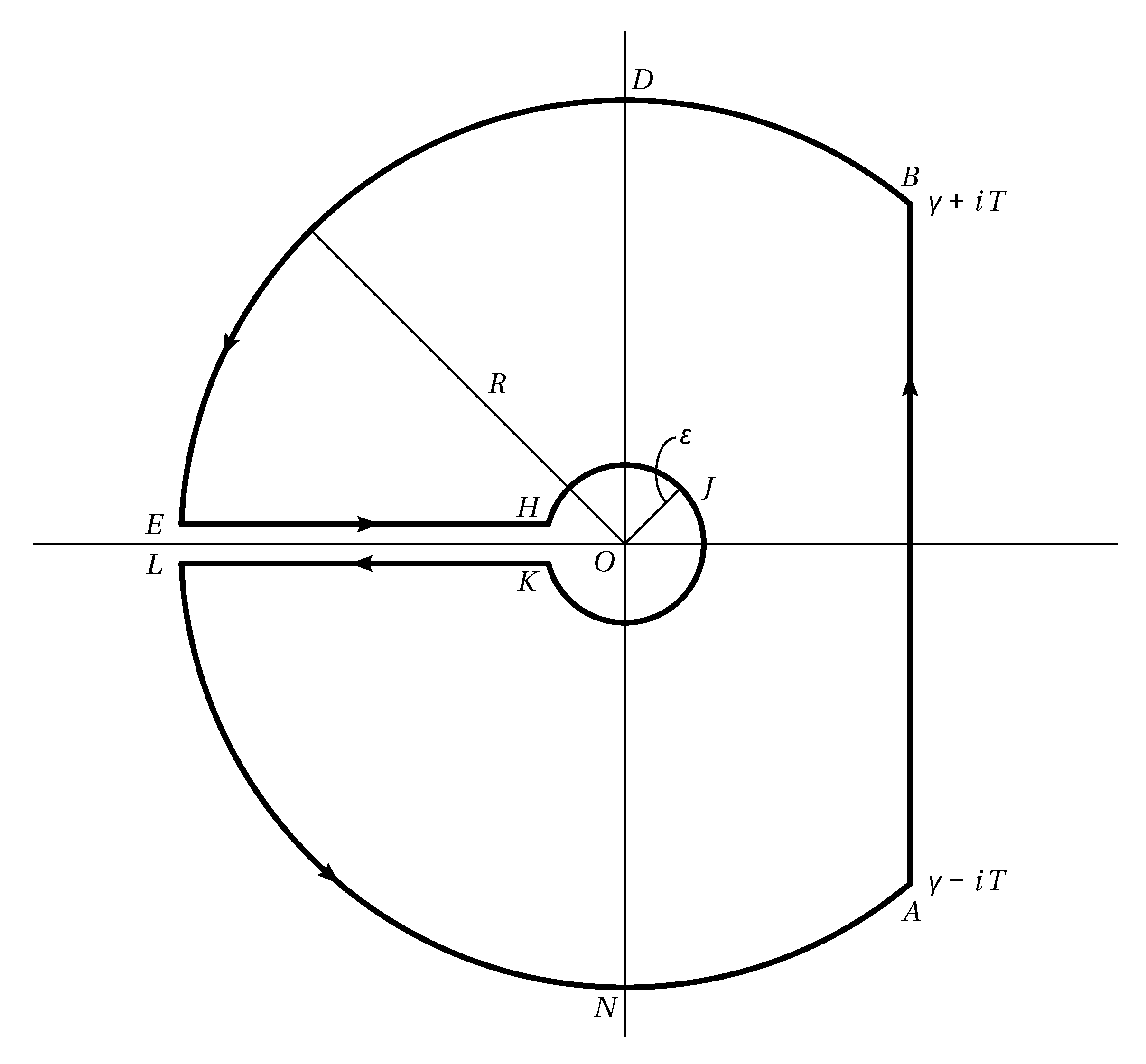
We can calculate the integral from (2) using residue theorem and appropriate integration contour. As function (3) branches at the origin, we need Bromwich contour (Figure 1) with $T=\sqrt{R^2-{\gamma }^2}$. It is clear that function (3) does not have poles inside the contour, then

$$\oint \frac{{\mathrm{e}}^{st}}{s^{\alpha }}\mathrm{d}s=0$$

(4)

Therefore, (simplified for clarity)

$$\underset{AB}{\int }+\underset{BDE}{\int }+\underset{EH}{\int }+\underset{HJK}{\int }+\underset{KL}{\int }+\underset{LNA}{\int }=0$$

(5)

If $R\to \infty$ then

$$\underset{AB}{\int }\frac{{\mathrm{e}}^{st}}{s^{\alpha }}\mathrm{d}s=\underset{\gamma -i\infty }{\overset{\gamma +i\infty }{\int }}\frac{{\mathrm{e}}^{st}}{s^{\alpha }}\mathrm{d}s$$

(6)

Thus,

$${\mathcal{L}}^{-1}\left(\frac{1}{s^{\alpha }}\right)=\underset{\begin{array}{c}R\to \infty \\ \epsilon \to 0\end{array}}{lim}-\frac{1}{2\pi i}\left(\underset{BDE}{\int }+\underset{EH}{\int }+\underset{HJK}{\int }+\underset{KL}{\int }+\underset{LNA}{\int }\right)$$

For $s=R{\mathrm{e}}^{i\theta }$, we have

$$\left|\frac{1}{s^{\alpha }}\right|=\frac{1}{R^{\alpha }}$$

(7)

then for $R\to \infty$, we have

$$\underset{BDE}{\int }=\underset{LNA}{\int }=0$$

(8)

It is necessary to calculate the rest of the integrals.

• Contour EH
  We substitute

  $$s=x{\mathrm{e}}^{\pi i}$$

  (9)
  Then,

  $$\begin{array}{cc}\hfill \mathrm{d}s=& -\mathrm{d}x\hfill \end{array}$$

  (10)

  $$\begin{array}{cc}\hfill s^{\alpha }=& x^{\alpha }(cos\alpha \pi +isin\alpha \pi )\hfill \end{array}$$

  (11)

  and changing s from $-R$ to $-\epsilon$ gives x from R to $\epsilon$. Then

  $$\begin{array}{cc}\hfill \underset{EH}{\int }\frac{{\mathrm{e}}^{st}}{s^{\alpha }}\mathrm{d}s=& \underset{-R}{\overset{-\epsilon }{\int }}\frac{{\mathrm{e}}^{st}}{s^{\alpha }}\mathrm{d}s=-\underset{R}{\overset{\epsilon }{\int }}\frac{{\mathrm{e}}^{-xt}}{x^{\alpha }}(cos\alpha \pi -isin\alpha \pi )\mathrm{d}x=\hfill \\ \hfill =& \underset{\epsilon }{\overset{R}{\int }}\frac{{\mathrm{e}}^{-xt}}{x^{\alpha }}(cos\alpha \pi -isin\alpha \pi )\mathrm{d}x\hfill \end{array}$$
• Contour HJK
  We substitute

  $$s=\epsilon {\mathrm{e}}^{\theta i},\theta \in [-\pi ,\pi ]$$

  (12)
  Then,

  $$\begin{array}{cc}\hfill \mathrm{d}s=& i\epsilon {\mathrm{e}}^{i\theta }\mathrm{d}\theta \hfill \end{array}$$

  (13)

  $$\begin{array}{cc}\hfill s^{\alpha }=& {\epsilon }^{\alpha }{\mathrm{e}}^{i\alpha \theta }\hfill \end{array}$$

  (14)

  and

  $$\underset{HJK}{\int }\frac{{\mathrm{e}}^{st}}{s^{\alpha }}\mathrm{d}s=\underset{-\pi }{\overset{\pi }{\int }}\frac{exp\left(\epsilon {\mathrm{e}}^{i\theta }t\right)}{{\epsilon }^{\alpha }{\mathrm{e}}^{i\alpha \theta }}i\epsilon {\mathrm{e}}^{i\theta }\mathrm{d}\theta =i{\epsilon }^{1-\alpha }\underset{-\pi }{\overset{\pi }{\int }}exp(i(1-\alpha )\theta +\epsilon {\mathrm{e}}^{i\theta }t)\mathrm{d}\theta$$
• Contour KL
  We substitute

  $$s=x{\mathrm{e}}^{-\pi i}$$

  (15)

  the

  $$\mathrm{d}s=-\mathrm{d}x$$

  (16)

  $$s^{\alpha }=x^{\alpha }(cos\alpha \pi -isin\alpha \pi )$$

  (17)

  and for s from $-\epsilon$ to $-R$ we have x from $\epsilon$ to R. Thus,

  $$\underset{KL}{\int }\frac{{\mathrm{e}}^{st}}{s^{\alpha }}\mathrm{d}s=\underset{-\epsilon }{\overset{-R}{\int }}\frac{{\mathrm{e}}^{st}}{s^{\alpha }}\mathrm{d}s==-\underset{\epsilon }{\overset{R}{\int }}\frac{{\mathrm{e}}^{-xt}}{x^{\alpha }}(cos\alpha \pi +isin\alpha \pi )\mathrm{d}x$$

After those calculations, we can take inverse Laplace transform, i.e.,

$$\begin{array}{cc}\hfill {\mathcal{L}}^{-1}\left(\frac{1}{s^{\alpha }}\right)=& \underset{\begin{array}{c}R\to \infty \\ \epsilon \to 0\end{array}}{lim}-\frac{1}{2\pi i}\left(\underset{\epsilon }{\overset{R}{\int }}\frac{{\mathrm{e}}^{-xt}}{x^{\alpha }}(cos\alpha \pi -isin\alpha \pi )\mathrm{d}x+\right.\hfill \\ \hfill +& i{\epsilon }^{1-\alpha }\underset{-\pi }{\overset{\pi }{\int }}exp(i(1-\alpha )\theta +\epsilon {\mathrm{e}}^{i\theta }t)\mathrm{d}\theta -\left.\underset{\epsilon }{\overset{R}{\int }}\frac{{\mathrm{e}}^{-xt}}{x^{\alpha }}(cos\alpha \pi +isin\alpha \pi )\mathrm{d}x\right)=\hfill \\ \hfill =& \underset{\begin{array}{c}R\to \infty \\ \epsilon \to 0\end{array}}{lim}\left(\frac{1}{2\pi i}2i\underset{\epsilon }{\overset{R}{\int }}\right.\frac{{\mathrm{e}}^{-xt}}{x^{\alpha }}sin\alpha \pi \mathrm{d}x-\left.\frac{i}{2\pi }i{\epsilon }^{1-\alpha }\underset{-\pi }{\overset{\pi }{\int }}exp(i(1-\alpha )\theta +\epsilon {\mathrm{e}}^{i\theta }t)\mathrm{d}\theta \right)=\hfill \\ \hfill =& \underset{0}{\overset{\infty }{\int }}\frac{sin\alpha \pi }{\pi }\frac{{\mathrm{e}}^{-xt}}{x^{\alpha }}\mathrm{d}x\hfill \end{array}$$

(18)

Taking Laplace transform of both sides of (18) implies thesis. □

This theorem is one of the variants of similar approaches. Grabowski in [19] proved the same result in a different way, generalizing to an entire class of diffusive realizations. As we have mentioned, the advantageous aspect is that the complex variable s is no longer explicitly raised to a non-integer power. We focus on this form of realization, as it gives the integrated function in the simplest form.

Applications of diffusive realization until recent years were mostly focused on theorem proving. For example, in [19] it was used to show that fractional integrator can stabilize an infinite dimensional system in a semigroup formalism. Moreover, it was shown that stability is non-exponential which is a non-trivial result in infinite dimensional system theory.

In the next section, we will show how to approximate diffusive realization using quadratures, which gives a new class of fractional systems approximations.

3. Approximation of Diffusive Realizations

We see that formula (1) does not include the complex variable risen to a non-integer power $\alpha$. The only variable that has a non-integer exponent is the auxiliary integrated variable x. Obviously the integration cannot be done analytically, because it would defeat the purpose—we would come back to a non-integer integrator. The main idea however is that because quadratures, generally approximate integrals by a sum of weighted values of integrated function at given points. In our case it would be

$$\underset{0}{\overset{\infty }{\int }}\frac{sin\alpha \pi }{\pi }\frac{1}{x^{\alpha }}\frac{1}{s+x}\mathrm{d}x\approx \sum _{i=0}^{n-1}\frac{b_i}{s+x_i}$$

(19)

where

$$\begin{array}{cc}\hfill b_i=& \frac{sin\alpha \pi }{\pi }\frac{w_i}{x_i^{\alpha }}\hfill \end{array}$$

(20)

and $x_i$, $w_i$ denote nodes and weights of quadrature, respectively, for approximation of other n.

This formulation is instantaneously advantageous for approximation, because the fractional integrator is represented as a sum of first order lags. This is, a simple form in the frequency domain but it is even better for time domain representation. State-space equations for 19 are (assuming natural y as output and u as control)

$$\begin{array}{cc}\hfill \dot{\mathbf{x}}\left(t\right)=& \mathbf{A}\mathbf{x}\left(t\right)+\mathbf{b}u\left(t\right)\hfill \\ \hfill y\left(t\right)=& {\mathbf{c}}^{\mathsf{T}}\mathbf{x}\left(t\right)\hfill \end{array}$$

(21)

where $\mathbf{A}=-\mathrm{diag}(a_0,\dots ,a_{n-1})$, $\mathbf{b}=\mathrm{col}(b_0,\dots ,b_{n-1})$ and $\mathbf{c}=\mathrm{col}(1,\dots ,1)$. As a continuous system is governed by a diagonal matrix, its discretization also will be diagonal, as long as discretization method is structure preserving (most well used methods like Euler, Tustin, and al-Alaoui have this property). Benefits of such structure are in detail explained in our earlier works [5,6,20].

Choosing a quadrature for approximation is not easy. In [21], the authors used the trapezoid rule. In [18], the rule of a rectangle with inhomogeneous nodes is considered. Both approaches convert the integration interval from $[0,\infty ]$ to $(0,{\omega }_{max}]$ as $x_{a}nd$ are only valid for high frequencies, but this causes integration errors, especially around ${\omega }_{max}$. Even though the integral (19) is defined over an infinite interval, many authors have considered limiting this interval to only the one that contains the frequency band of interest.

In this paper, we want to consider the following approaches (expanding on our earlier conclusions from [14,15]:

• Create approximation directly from integral on an unbounded domain using Gauss–Laguerre quadrature.
• Create approximation from on an unbounded domain using variable change, which results in Fourier–Chebyshev quadrature.
• Create approximation on a bounded domain, but on a logarithmic scale using Clenshaw–Curtis and Gauss–Legendre quadratures.

The purpose of using a logarithmic scale is to provide balance frequency representation for different orders of magnitude. We obtain that through substitution:

$$x={10}^{\theta }$$

Integration (1) for $x\in [{10}^a,{10}^b]$ reduces to

$$\underset{a}{\overset{b}{\int }}\frac{sin\alpha \pi }{\pi }log\left(10\right){10}^{\theta (1-\alpha )}\frac{1}{s+{10}^{\theta }}\mathrm{d}\theta .$$

(22)

In the following section, we describe quadrature formulas we use.

4. Quadrature Formulas

4.1. Gauss–Laguerre Quadrature

Gauss–Laguerre quadrature computes integrals of form

$$\underset{0}{\overset{\infty }{\int }}{x}^{\alpha }{\mathrm{e}}^{-x}f\left(x\right)\mathrm{d}x$$

(23)

with use of

$$\sum _{k=0}^N{w}_k^{L}f\left(x_k^L\right)$$

(24)

where nodes $x_j^L$ are poles of generalized Laguerre polynomial given by (see in [22])

$$L_N^{\alpha }=\sum _{m=0}^N{(-1)}^m\left(\begin{array}{c}N+\alpha \\ N-m\end{array}\right)\frac{x^m}{m!}$$

(25)

and $w_j^L$ are defined as

$$w_j^L=\frac{\Gamma (N+\alpha +1)x_j^L}{N!{\left[(N+1)L_{N+1}^{\alpha }\left(x_j^L\right)\right]}^2}$$

(26)

This quadrature is notoriously numerically fragile, and there are problems with computing weights and nodes for high orders [23]. It is however one of the only quadratures defined using orthogonal functions on $L^2[0,\infty ]$.

4.2. Clenshaw Curtis and Fourier–Chebyshev Quadrature

Those quadratures are interpolating quadratures based on Chebyshev nodes of second kind.

In modern analysis Clenshaw–Curtis quadrature is an interpolation quadrature on Chebyshev nodes. In certain aspects, it is also equivalent to discrete cosine transform, and can be computed using FFT. In the Clenshaw–Curtis quadrature, the nodes have the form

$$x_j^{CC}=cosj\frac{\pi }{n},j=0,1,...,n$$

(27)

$${\mathbf{w}}^{CC}=\left[\begin{array}{cccc}{w}_0^{CC}& w_1^{CC}& \cdots & w_n^{CC}\end{array}\right]$$

(28)

$${\mathbf{w}}^{*}=\mathrm{ifft}(\mathbf{g}+\mathbf{v})$$

(29)

where: $\mathbf{v}={\left[v_k\right]}_{1\times n+1}$, $\mathbf{g}={\left[g_k\right]}_{1\times n+1}$

$$\left\{\begin{array}{ccc}{v}_k& =& \frac{2}{1-4k^2},k=0,1,...,\left[\begin{array}{c}\frac{n}{2}\end{array}\right]-1\\ v_{[n/2]}& =& \frac{n-3}{2[n/2]-1}-1\\ v_{n-k}& =& v_k,k=1,2,...,\left[\begin{array}{c}\frac{n-1}{2}\end{array}\right]\end{array}\right.$$

(30)

$$\left\{\begin{array}{ccc}{g}_k& =& -w_0^{CC},k=0,1,...,\left[\begin{array}{c}\frac{n}{2}\end{array}\right]-1\\ v_{[n/2]}& =& w_0^{CC}[(2-\mathrm{mod}(n,2))n-1]\\ v_{n-k}& =& g_k,k=1,2,...,\left[\begin{array}{c}\frac{n-1}{2}\end{array}\right]\end{array}\right.$$

(31)

and $w_0^{CC}={(n^2-1+\mathrm{mod}(n,2))}^{-1}$.

The advantage of this quadrature is a very low computational complexity of determining the coefficients, equal to the complexity of the fast Fourier transform.

Fourier–Chebyshev quadrature is generally equivalent to Clenshaw–Curtis. The main differences are their derivation and integration interval ([−1, 1] for Clenshaw–Curtis and [0, $\pi$] for Fourier–Chebyshev). In this section, we consider a variant of the Fourier–Chebyshev quadrature proposed by Boyd [24]. It extends the integration domain to an unbounded one. It is done by transformation

$$x=L{\mathrm{ctg}}^2(t/2)$$

(32)

which maps interval [0, $\pi$] to [0, ∞], where L is a given constant. This yields

$$\underset{0}{\overset{\infty }{\int }}f\left(x\right)\mathrm{d}x=\underset{0}{\overset{\pi }{\int }}2Lf\left(L{\mathrm{ctg}}^2(t/2)\right)\frac{sint}{{(1-cost)}^2}\mathrm{d}t$$

(33)

Therefore, the quadrature takes form of sum

$$\sum _{k=1}^N{w}_k^{FC}f\left(x_k^{FC}\right)$$

(34)

where

$$\begin{array}{cc}\hfill x_j^{FC}=& L{\mathrm{ctg}}^2\left(\frac{t_j}{2}\right)\hfill \end{array}$$

(35)

$$\begin{array}{cc}\hfill w_j^{FC}=& \frac{2Lsin{t}_j}{{(1-cos{t}_j)}^2}\frac{2}{N+1}\sum _{m=1}^N\frac{sinm{t}_j(1-cosm\pi )}{m}\hfill \end{array}$$

(36)

$$\begin{array}{cc}\hfill t_j=& \frac{\pi j}{N+1}\hfill \end{array}$$

(37)

4.3. Gauss–Legendre Quadrature

Gauss quadrature, also known as Gauss–Legendre quadrature, is a quadrature where the nodes are the roots of Legendre polynomials.

The main advantage of the Gauss–Legendre quadrature comes from the orthogonality of Legendre polynomials. In particular, let us consider a polynomial $p\left(x\right)$ of order $2N+1$. Such a polynomial can always be written as $p\left(x\right)=q\left(x\right)·l_{N+1}\left(x\right)+r\left(x\right)$, where $q\left(x\right)$ is a polynomial of degree $N+1$, $l_{N+1}\left(x\right)$ is a Legendre polynomial of degree $N+1$ and $r\left(x\right)$ is a polynomial of degree N. When considering interpolation quadrature of degree $N+1$ on nodes, we can easily see that ${\int }_{-1}^{1}q\left(x\right)·l_N\left(x\right)\mathrm{d}x=0$ because of orthogonality of Legendre polynomials and the integral of $r\left(x\right)$ is exact because of uniqueness of interpolation polynomials. These facts give that Gauss–Legendre quadratures on $N+1$ nodes are exact for polynomials of order $2N+1$. In the case of Gauss–Legendre quadrature, these formulas for weights are, respectively,

$$x_j^{GL}=\lambda \left(T\right),w_j^{GL}=2v_{1j}^2$$

(38)

where:

$$T=\frac{1}{2}\left[\begin{array}{cccccc}0& \frac{1}{\sqrt{1-2^{-2}}}& 0& \cdots & 0& 0\\ \frac{1}{\sqrt{1-2^{-2}}}& 0& \frac{1}{\sqrt{1-3^{-2}}}& \cdots & 0& 0\\ 0& \frac{1}{\sqrt{1-3^{-2}}}& 0& \cdots & 0& 0\\ ⋮& ⋮& ⋮& \ddots & ⋮& ⋮\\ 0& 0& 0& \cdots & 0& \frac{1}{\sqrt{1-n^{-2}}}\\ 0& 0& 0& \cdots & \frac{1}{\sqrt{1-n^{-2}}}& 0\end{array}\right]=V\mathrm{diag}\left(\lambda \left(T\right)\right)V^{-1}$$

(39)

and $V={\left[v_{ij}\right]}_{n\times n}$.

Gauss quadratures, thanks to orthogonality, are exact for polynomials of twice higher order than other interpolation quadratures. In practice Clenshaw–Curtis quadrature offers very similar precision [25]. Moreover, it has much smaller computational complexity. It should be also noted, that while based on interpolation both of these quadratures are immune to Runge’s phenomenon, as both Legendre and Chebyshev nodes have asymptotic distribution of $1/\sqrt{1-x^2}$ for $[-1,1]$ interval.

5. SoftFRAC Library to Realization Fractional Order Dynamic Elements

We can easily implement quadrature-based approximations in SoftFrac library. SoftFRAC is metalanguage software to approximate non-integer dynamic elements in MATLAB^®, Python and C. Currently it offers functionality to create state-space fractional model and transfer function fractional model of the non-integer dynamic element $\frac{1}{s^{\alpha }}$ based on approximations described in the previous section.

Either low accuracy or lack of numerical stability characterizes competing (and available in open source form) software. SoftFRAC relies on algorithms developed as part of the completed project, which are characterized by high numerical robustness and scalable accuracy. We identified the initial potential recipients as academic entities (supporting research on fractional differential equations and methods of designing control systems) and innovative industry (new methods of signal processing and robust control).

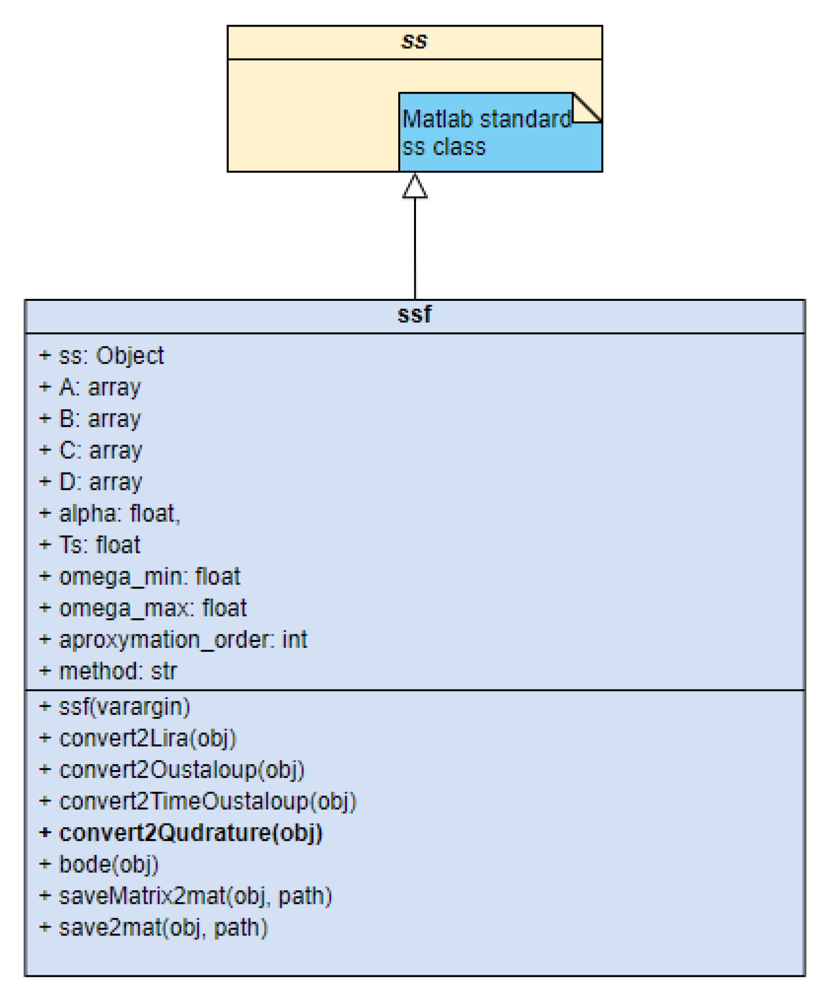
State-space fractional model class (ssf) inherits from the MATLAB^® Control Systems Toolbox^TM state-space model class (ss) and has all functionality of this class. Similarly, transfer function fractional model class (ssf) inherits form transfer function model. In both cases variables describing approximation extend standard object properties:

• ss - base MATLAB^® object,
• A, B, C, D - matrix containing approximation parameters
• alpha - derivative order,
• omega_min - approximation frequency lower band,
• omega_max - approximation frequency upper band,
• approximation_order - approximation order
• method - name of approximation method

The Object-oriented programming (OOP) paradigm ensures the best quality of software and the possibility of its further development. OOP refers to a computer programming in which programmers define not only the data type of data structure, but also the operations (functions) that can apply to the data structure. This approach improves the ability to manage software complexity, which is particularly important when developing and maintaining large applications and data structures. The concepts and rules used in object-oriented programming provide these important benefits:

• Inheritance is the concept allowing defining subclasses of data objects that share some or all of the main class characteristics. This property of OOP reduces development time and ensures more accurate coding.
• Class defines only the data it needs to be concerned with. This protects running instance of the class (an object) from accidentally accessing other program data.
• The concept of data classes allows the programmer to create any new data type that is not already defined in the language itself.

OOP capabilities of the MATLAB^® language enable developing complex technical computing applications. In the MATLAB^® environment we can define classes and apply standard object-oriented design patterns, inheritance, encapsulation, and reference behavior without engaging in the low-level housekeeping tasks required by other languages.

In SoftFRAC classes we implemented the method of conversion between different the approximation methods described in the previous. Because we used inheritance mechanism in the implementation. The user can use all functionalities of parent classes ss and tf. In particular, the user can use this realization to Simulink^® simulation, system behavior analysis, and easy plotting of dynamic characteristics. We have added to the classes a construction method for easy conversion between those types, from ssf to tff, and vice versa. We present the UML diagram of the ssf class implementation in Figure 2.

Implementation Analysis

Table 1. Time run and memory performance comparison for proposed methods.

	Approximation Order	10	100	1000	10,000
Gauss–Laguerre quadrature	time [s]	0.40	0.44	11.04	869.73
	memory [Kb]	3,162,112	3,158,016	8,019,968	801,566,720
Clenshaw–Curtis quadrature	time [s]	0.03	0.007	0.028	1.90
	memory [Kb]	3,162,112	3,158,016	8,019,968	801,566,720

presents a comparison of the time and memory needed to calculate the discussed approximations in MATLAB^®.

For low orders of approximation, the memory needed to represent them does not differ significantly from each other. Here, the main memory user is the environment. With high orders, the differences in memory are noticeable and result from the number of elements describing the approximation. Both methods need the same amount of memory to function. Because of the execution time, the Clenshaw–Curtis quadrature method is much faster in all cases.

Finally, the system generated by these methods generates a diagonal matrix. This means that the use of such systems in control or filtering processes to calculate the next step requires only $O\left(n\right)$ (approximation order) operations, advantageous compared to typical $O\left(n^2\right)$.

6. Approximation Analysis

In order to analyze the approximation performance, we conducted error analysis using $H^{\infty }$ norm. We considered the difference

$$e\left(s\right)=\frac{1}{s^{\alpha }}-\sum _{i=0}^n\frac{b_i}{s+x_i}$$

for frequency $[{10}^{-5},{10}^5]$ rad/s. We increased the order of quadrature in order to observe the change of norm of ${\parallel e\parallel }_{\infty }$. We illustrate tests for $\alpha =1/2$ but there are systematic for all orders $\alpha \in (0,1)$.

In the following subsections, we will discuss exemplary results of the approximation analysis. We divided them into infinite and finite intervals.

6.1. Infinite Intervals

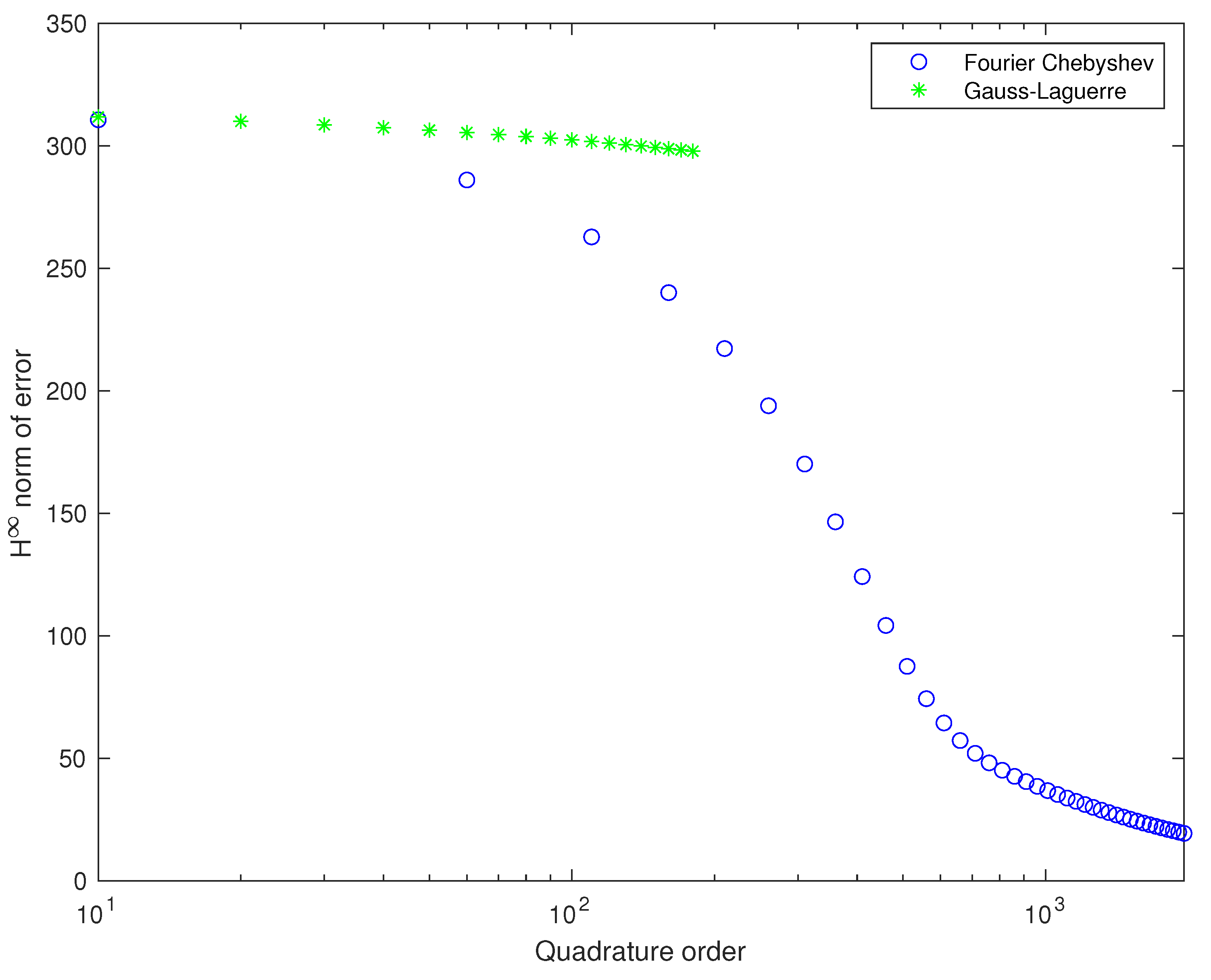
We increased the order of quadrature in order to observe the change of norm of ${\parallel e\parallel }_{\infty }$. In the Figure 3 we depicted this analysis. In the figure, we see quite slow convergence (especially linear). We computed Laguerre–Gauss quadrature only up to 180 order because of its numerical instability. Calculating the poles of Laguerre polynomials is also a known problem [26].

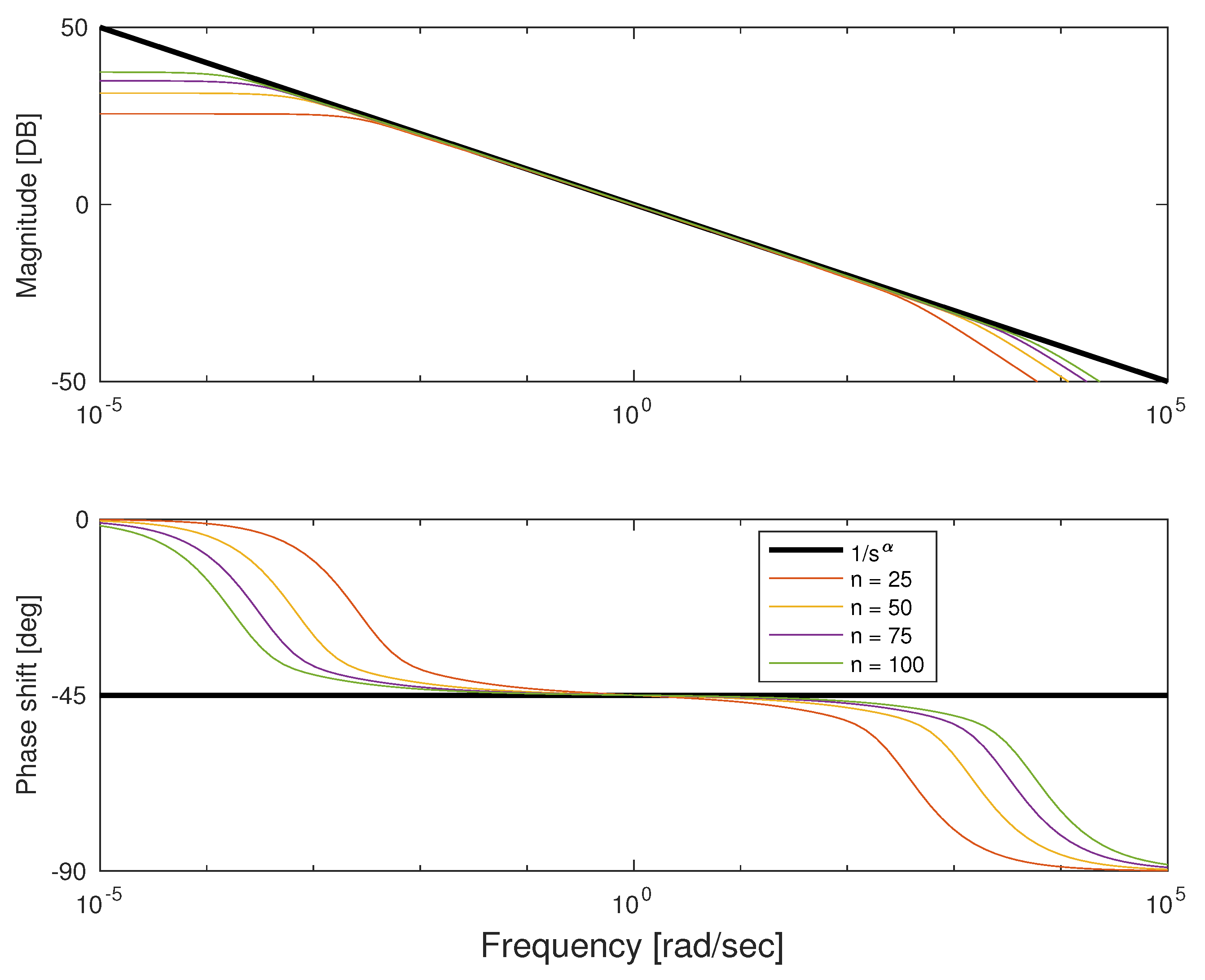
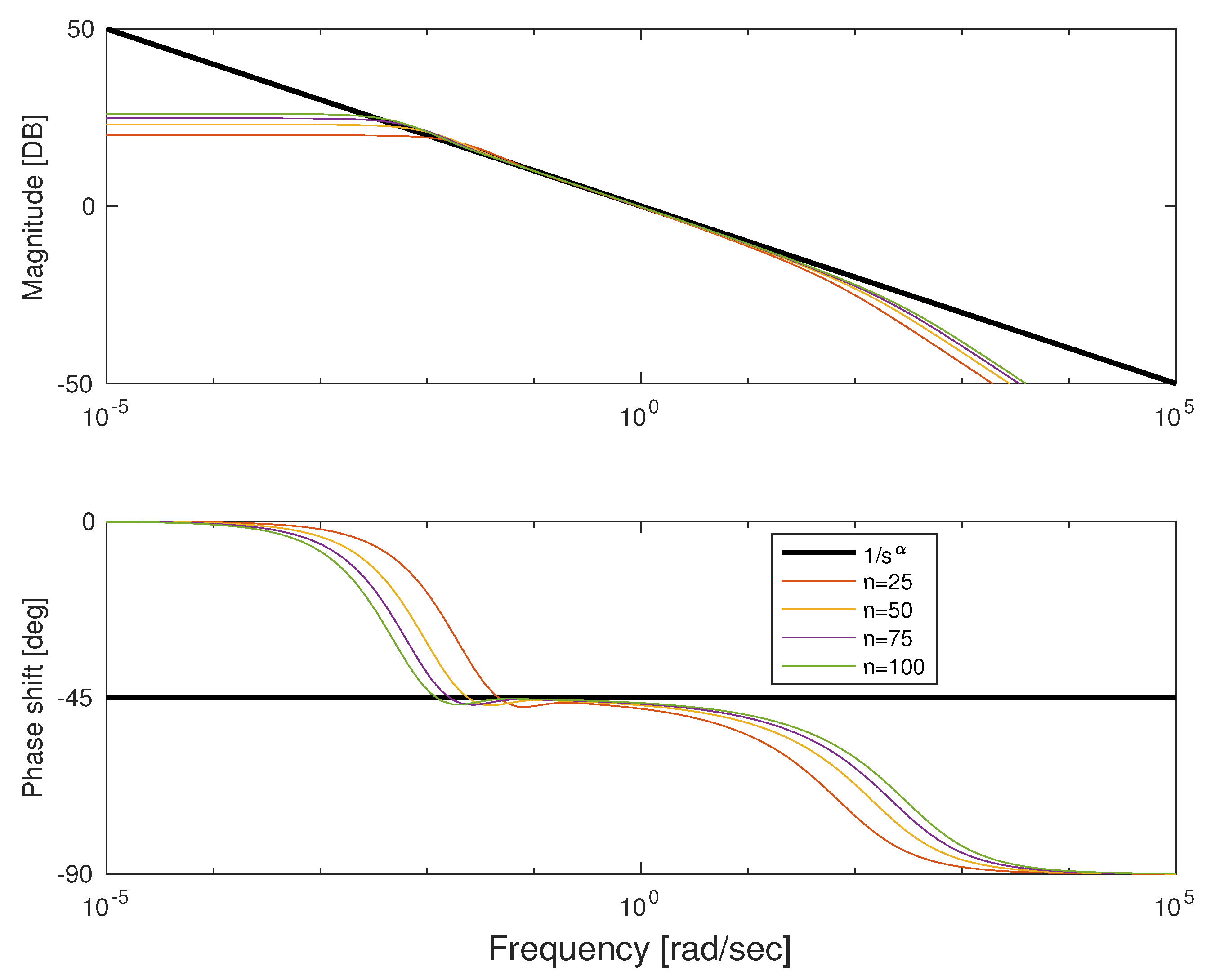
We conducted also a detailed analysis of Bode plots for both types of quadratures. In Figure 4 and Figure 5, we depicted the characteristics for frequency $[{10}^{-5},{10}^5]$ rad/s and approximation order ranging from 25 to 100. We can see that both approximations show good fitness in the middle of frequency interval and errors on both ends. The error for low frequencies in natural because it is impossible to get infinite gain with a finite number of first-order lag systems. Similarly, the error for higher frequencies results from the difference between order of numerator and denominator of approximation. Because transfer function is strictly proper, it damps high frequencies at least 20 db/dec. Note that for Fourier–Chebyshev quadrature, the interval of fitness is wider.

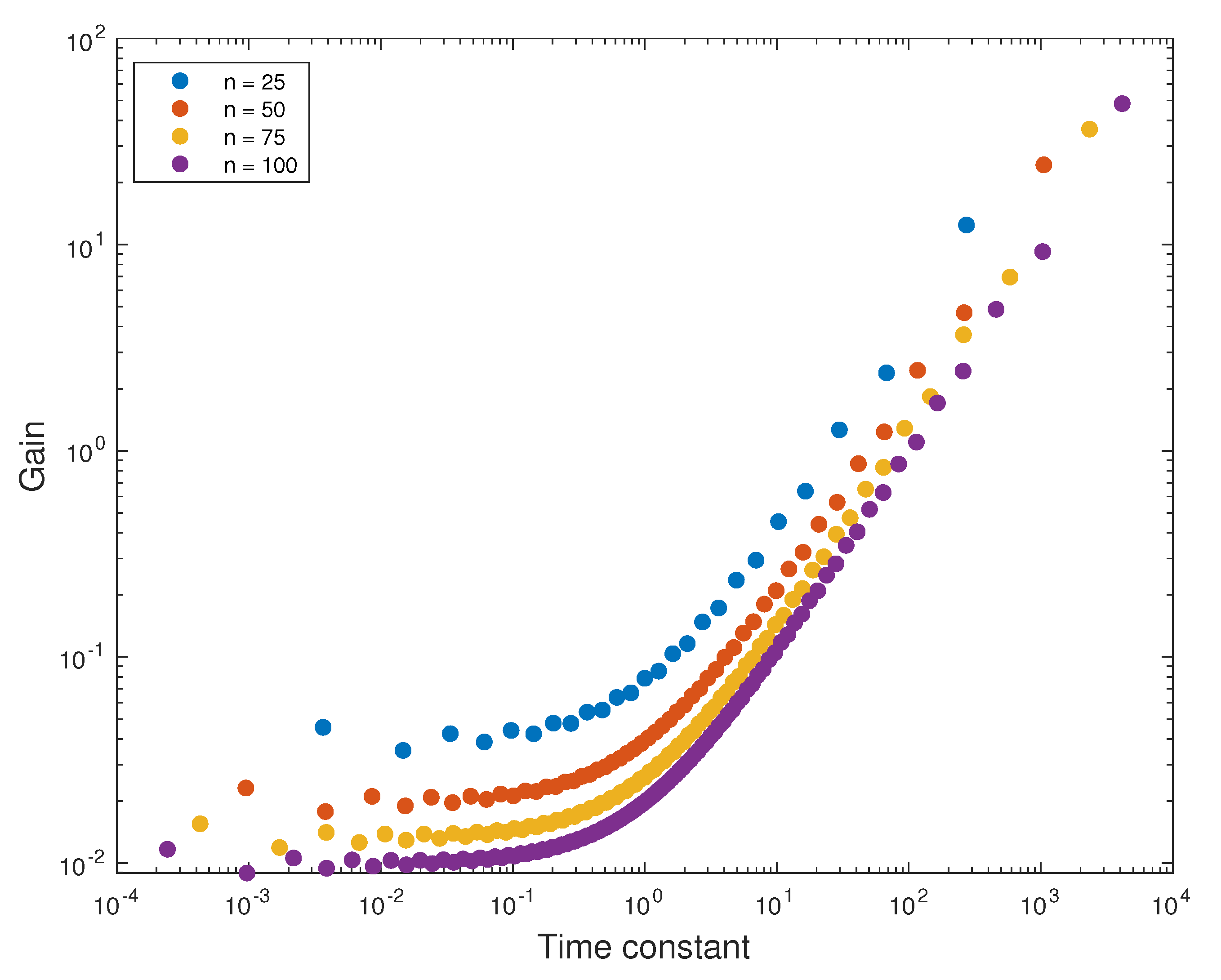
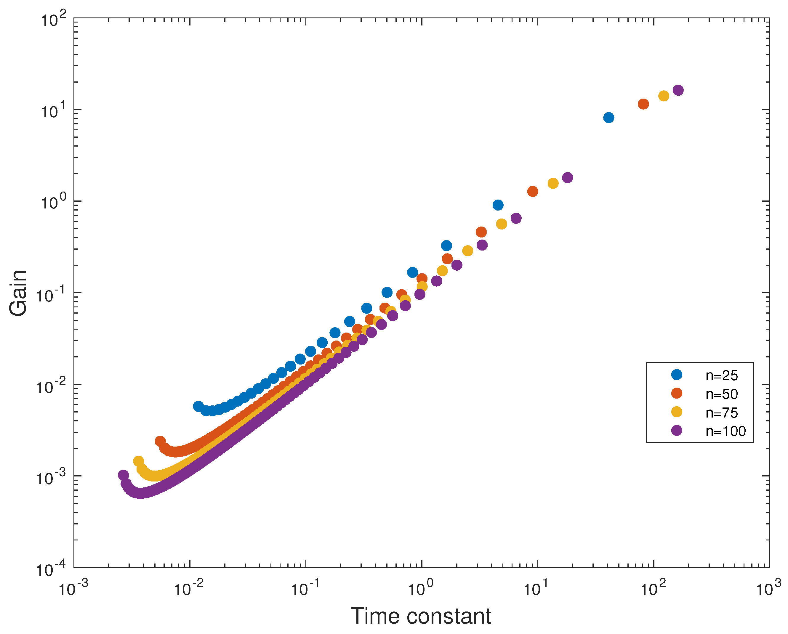
We can observe the cause of such fit in Figure 6 and Figure 7. Their (for various orders) gains are presented as a function of time constant for the terms of approximating sum (19). We can see that for Fourier–Chebyshev we have the most time constants between 1/10 and 10 s (it increases with increasing approximation order). In case of Gauss–Laguerre quadrature, the time constants are gathered around 0.01 s. Moreover, for Fourier–Chebyshev the time constants cover wider range of frequencies for the same approximation order. The difference between the smallest and largest time constant is 4 decades in comparison with 8 for Fourier–Chebyshev. It can be also seen that the biggest gain is for the longest time constant.

6.2. Finite Intervals

For finite interval quadratures, we have tested both Gauss–Legendre and Clenshaw–Curtis simultaneously. We did our testes for the integration intervals of $[-5,5]$ and $[-7,7]$, which correspond to frequency ranges of $[{10}^{-5},{10}^5]$ and $[{10}^{-7},{10}^7]$, respectively.

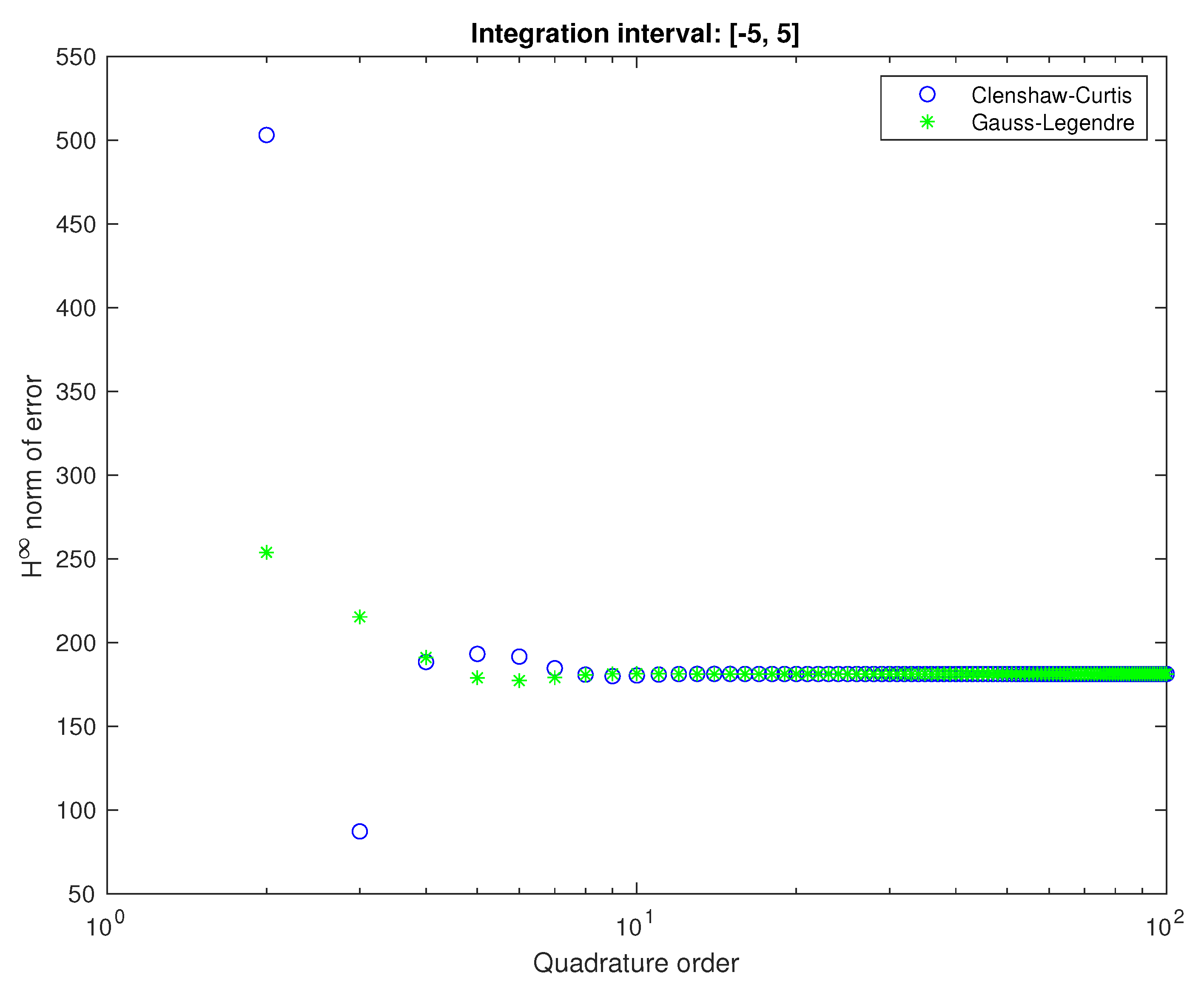
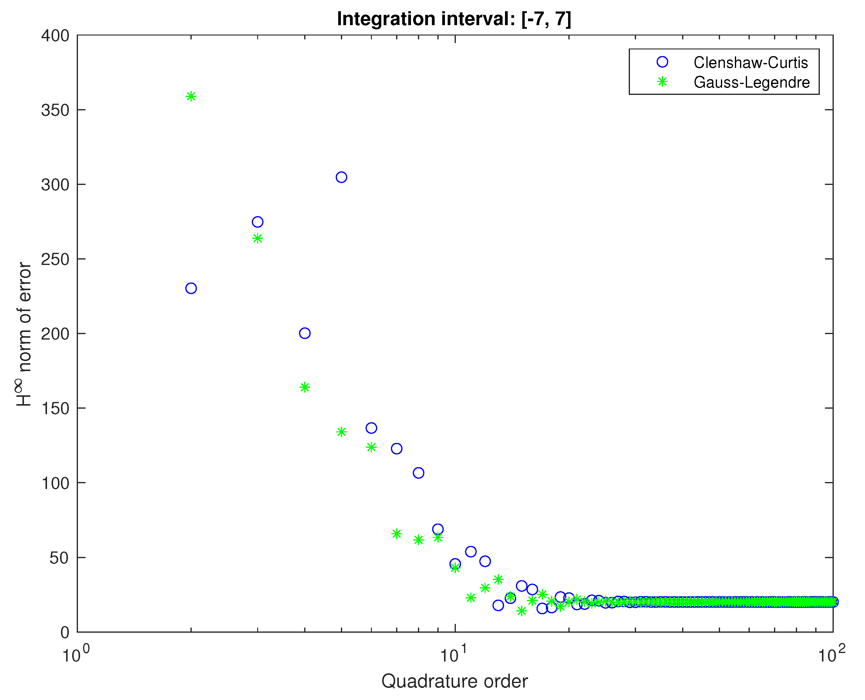
For initial analysis we have considered the integration interval of $[-5,5]$ for (22) corresponding to $[{10}^{-5},{10}^5]$ rad/s for original integral. In Figure 8, we depicted this analysis. After initial convergence, the error stops decreasing and fixes on a certain value. The limitation of an infinite interval causes this error into a finite one. Indeed, one can observe in the Figure 9 that increasing the interval to $[-7,7]$ results in dropping of error by an order of magnitude. For both intervals we can observe rather quick stabilization of approximation error. The low error for Clenshaw–Curtis quadrature of low order is caused by an artifact of oscillating phase error for high gains.

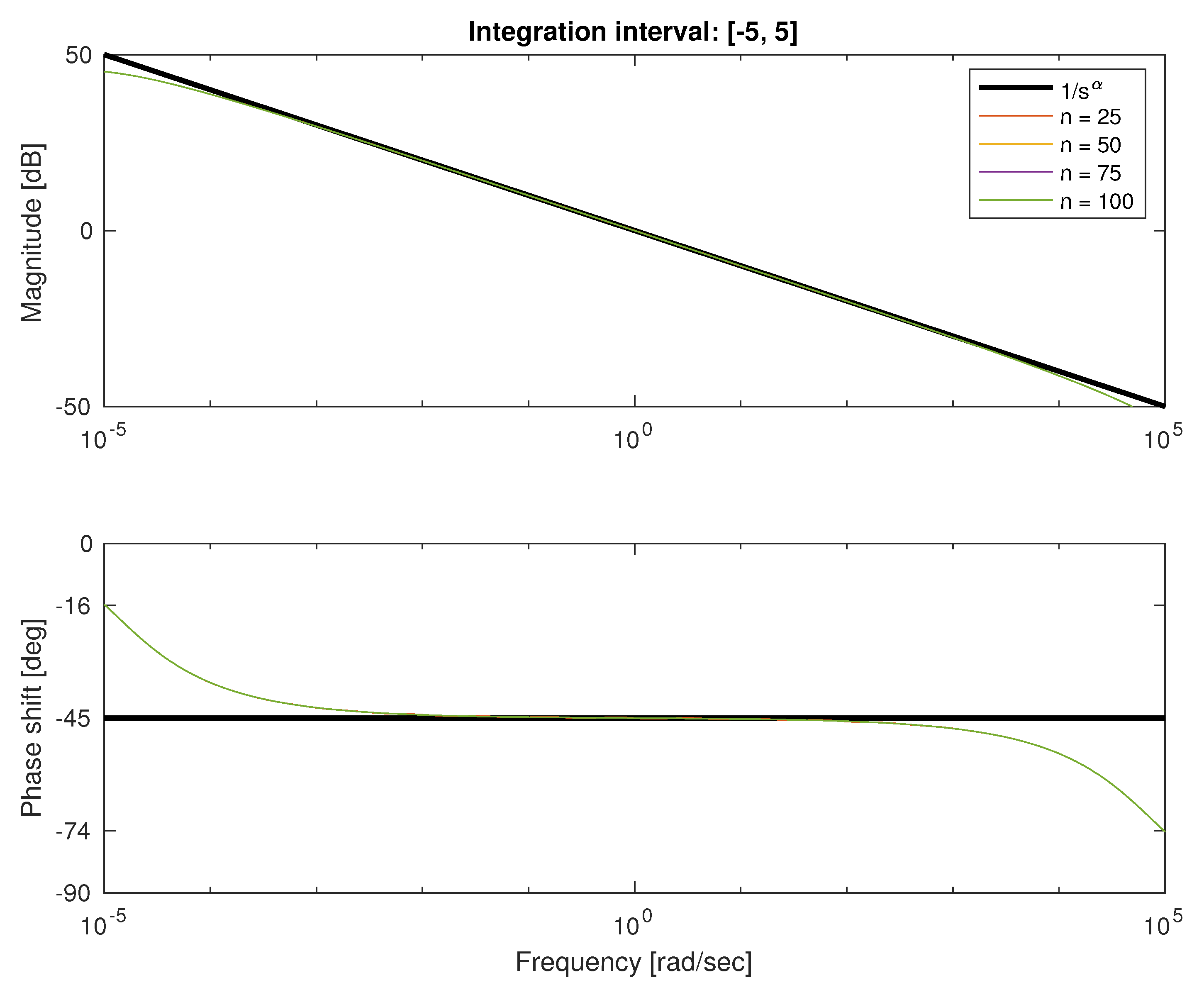
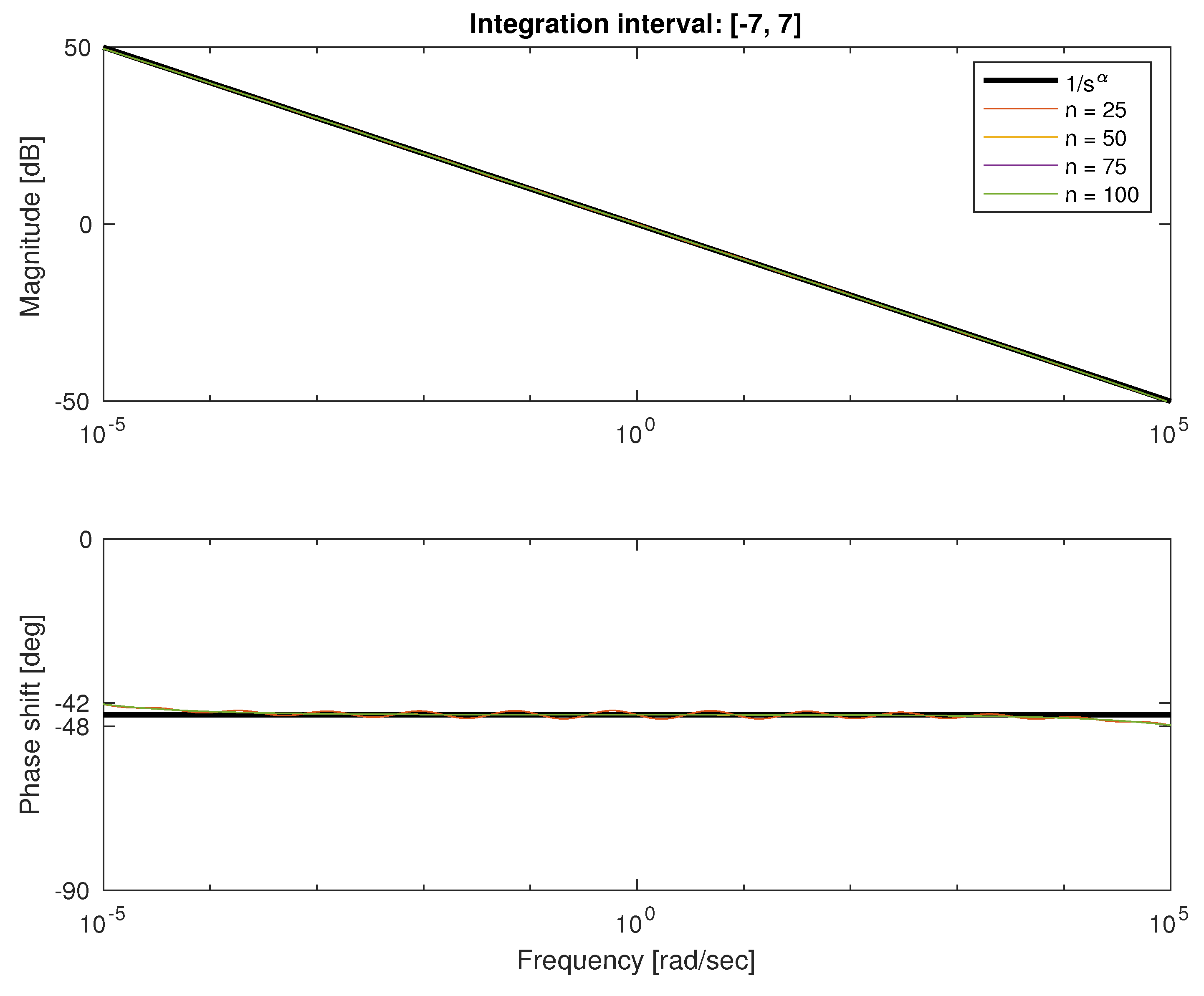
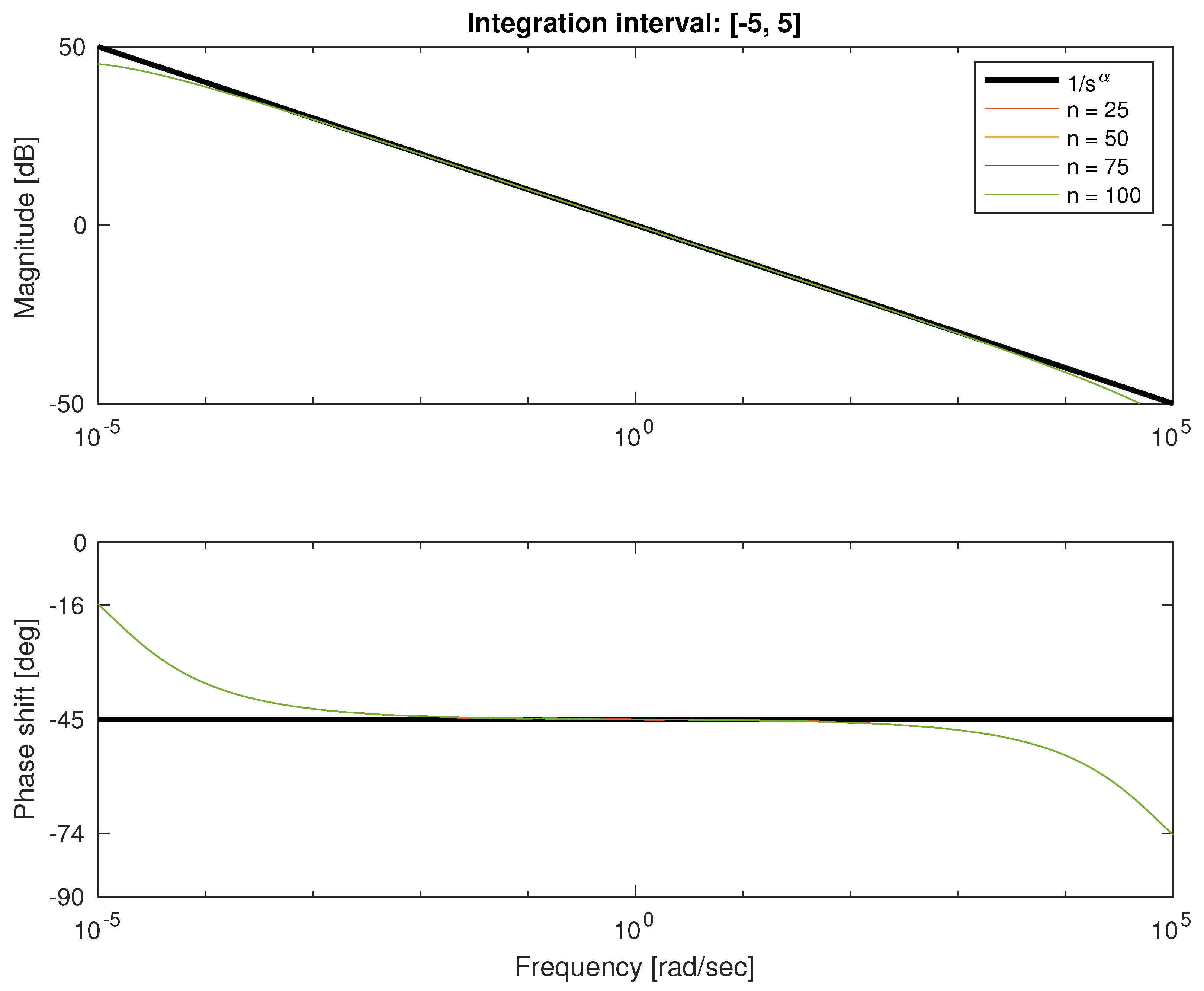
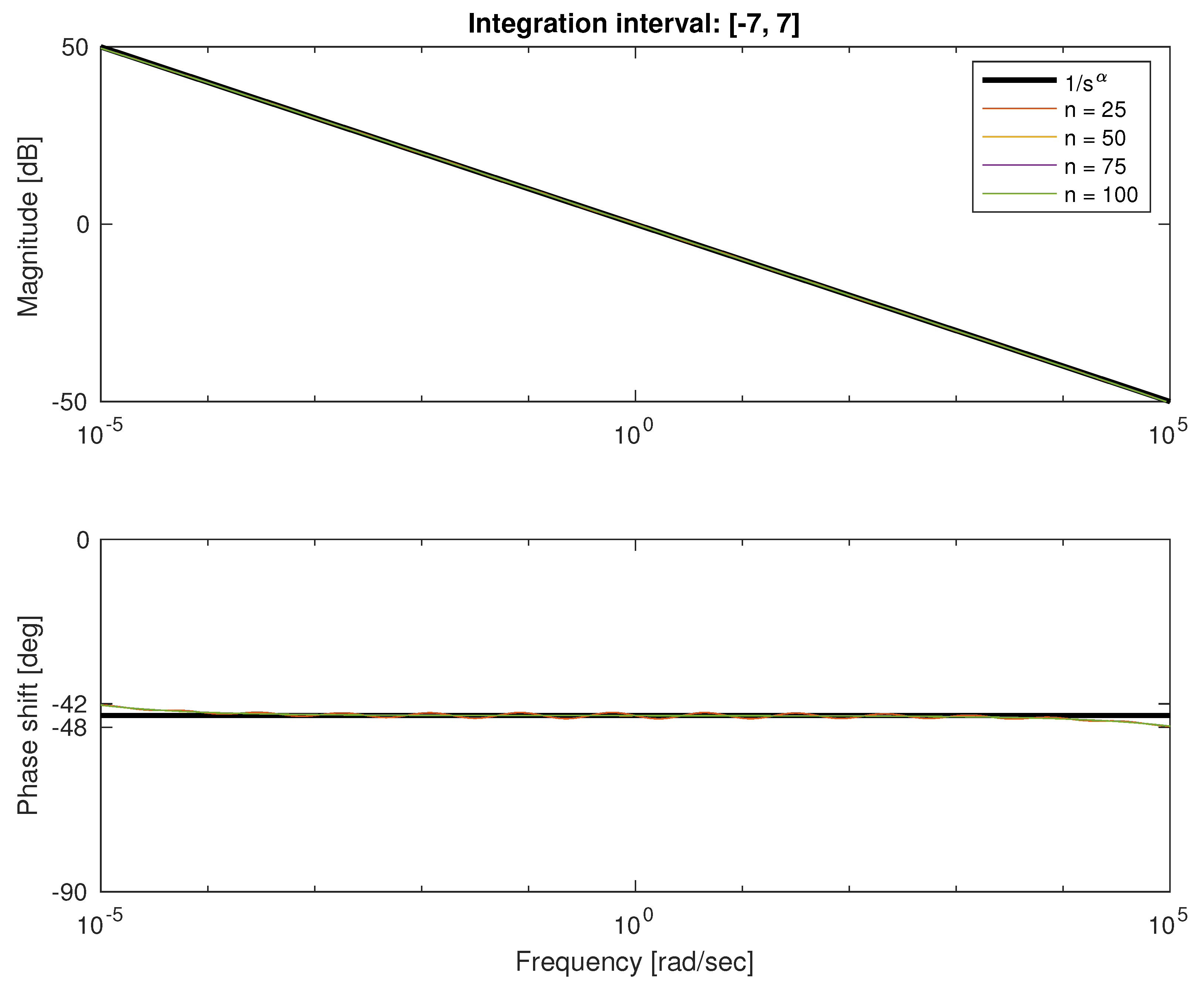
The cause of the fixed error is the phase errors at low frequencies. We can observe it on the Bode plots in Figure 10, Figure 11, Figure 12 and Figure 13. Bounded domain approximations are much better than unbounded ones, and for high orders on wider domains are practically indistinguishable, with phase errors of $\pm 2^{\circ }$. We can however see that these errors are not vanishing, and because of large low-frequency gains are dominating.

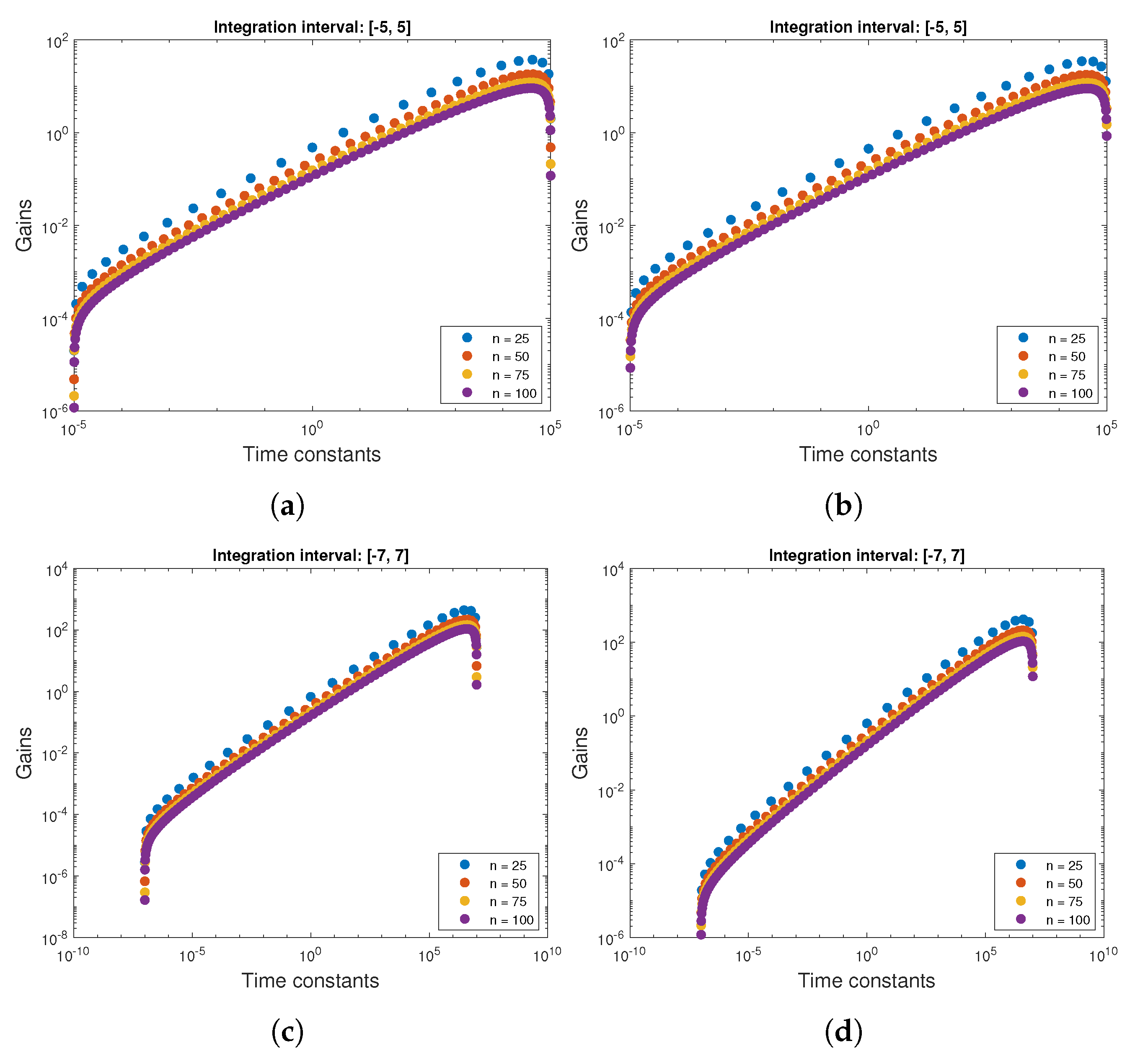
To consider the differences between quadratures, we can compare the gain-time constant pairs illustrated in the Figure 14. Both quadratures generate practically indistinguishable approximations for higher orders. Gains and time constants are also similarly distributed. This, however, does not explain the issues with low-frequency behavior, which we will address in the next section.

7. Discussion of Low Frequency Behavior

We can trace the issues with problems of uneven approximation over the frequency interval to Bernstein theorem.

Theorem 1

(Bernstein). Let a function f analytic in $[-1,1]$ be analytically continuable to the open Bernstein ellipse $E_{\rho }$, where it satisfies $\left|f\right(x\left)\right|\le M$ for some M. Chebyshev interpolants $p_n$ of f satisfy

$$\parallel f-p_n\parallel \le \frac{4M{\rho }^{-n}}{\rho -1}$$

where ρ is the length of the semi-major axis of $E_{\rho }$ plus the length of the semi-minor axis.

For Chebyshev polynomial projections, the bound is twice smaller, and for Legendre polynomial projections, the result is similar.

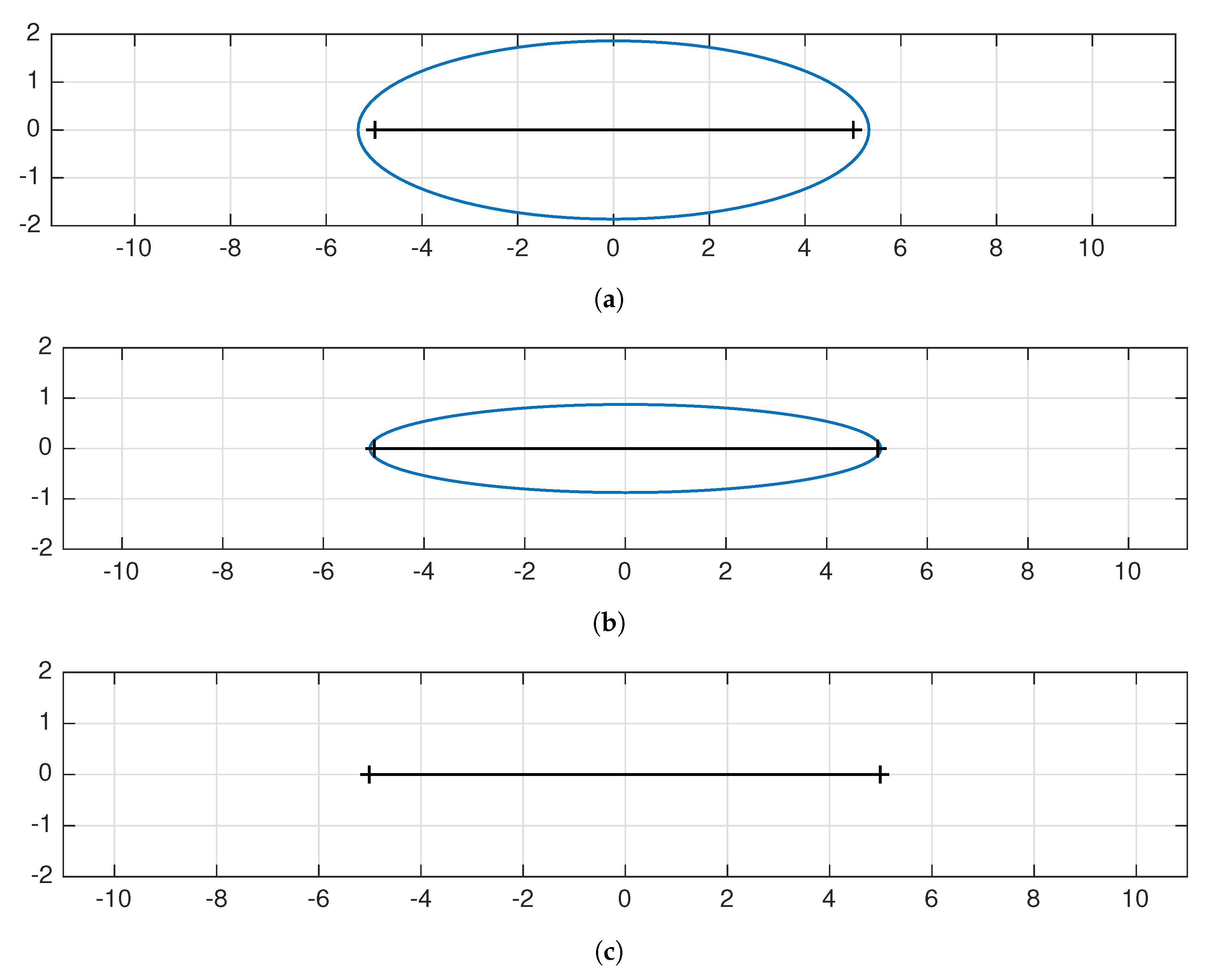
We can observe that we compute definite integral of analytic function for each frequency value. For all frequencies, in the bounded domain that function is analytic in certain Bernstein ellipse, i.e., ellipse with foci in edges of integration interval. However, while frequencies are approaching towards zero the analyticity ellipse shrinks. Because of that $\rho$ constant is rapidly approaching 1, reducing order of convergence. We can observe it in the Figure 15, where we can see that while there is no problem for high and mid frequencies (Figure 15b,c) for frequencies such as ${10}^{-5}$ rad/s ellipse shrinks to the interval itself.

8. Conclusions

In this paper, we have presented results considered practical application of diffusive realization of fractional order integration. With no doubt, the bounded domain methods are more efficient, however they introduce a fixed approximation error. That error arises from the problems with analyticity of integrated function around zero. In SoftFrac, we implement the entire approximation scheme with both Gauss–Legendre and Clenshaw–Curtis methods. If however we will determine more efficient quadrature rule, extensions are readily available. Moreover, the open license for academic users will allow introducing it also easily. We can find all the details about SoftFrac on the package website: http://non-integer.pl (accessed on 23 July 2021).

References

- Oustaloup, A.; Levron, F.; Mathieu, B.; Nanot, F.M. Frequency-band complex noninteger differentiator: Characterization and synthesis. Circuits Syst. I Fundam. Theory Appl. IEEE Trans. 2000, 47, 25–39. [Google Scholar] [CrossRef]
- Petráš, I. Fractional-Order Nonlinear Systems: Modeling, Analysis and Simulation. In Nonlinear Physical Science; Springer: Berlin/Heidelberg, Germany, 2011. [Google Scholar]
- Podlubny, I. Fractional Differential Equations: An Introduction to Fractional Derivatives, Fractional Differential Equations, to Methods of Their Solution and Some of Their Applications. In Mathematics in Science and Engineering; Elsevier: Amsterdam, The Netherlands, 1998. [Google Scholar]
- Piątek, P.; Zagórowska, M.; Baranowski, J.; Bauer, W.; Dziwiński, T. Discretisation of different non-integer order system approximations. In Proceedings of the Methods and Models in Automation and Robotics (MMAR), 2014 19th International Conference on IEEE, Miedzyzdroje, Poland, 2–5 September 2014; pp. 429–433. [Google Scholar]
- Baranowski, J.; Bauer, W.; Zagórowska, M.; Dziwiński, T.; Piątek, P. Time-domain Oustaloup Approximation. In Proceedings of the Methods and Models in Automation and Robotics (MMAR), 2015 20th International Conference On IEEE, Miedzyzdroje, Poland, 24–27 August 2015; pp. 116–120. [Google Scholar]
- Baranowski, J.; Bauer, W.; Zagórowska, M. Stability Properties of Discrete Time-Domain Oustaloup Approximation. In Theoretical Developments and Applications of Non-Integer Order Systems; Domek, S., Dworak, P., Eds.; Springer: Berlin/Heidelberg, Germany, 2016; Volume 357, pp. 93–103. [Google Scholar] [CrossRef]
- Bania, P.; Baranowski, J.; Zagórowska, M. Convergence of Laguerre Impulse Response Approximation for Non-Integer Order Systems. Math. Probl. Eng. 2016, 2016, 9258437. [Google Scholar] [CrossRef]
- Stanisławski, R.; Latawiec, K.J.; Gałek, M.; Łukaniszyn, M. Modeling and Identification of Fractional-Order Discrete-Time Laguerre-Based Feedback-Nonlinear Systems. In Advances in Modelling and Control of Non-integer-Order Systems; Latawiec, K.J., Łukaniszyn, M., Stanisławski, R., Eds.; Springer: Berlin/Heidelberg, Germany, 2015; Volume 320, pp. 101–112. [Google Scholar]
- De Keyser, R.; Muresan, C.; Ionescu, C. An efficient algorithm for low-order direct discrete-time implementation of fractional order transfer functions. ISA Trans. 2018, 74, 229–238. [Google Scholar] [CrossRef] [PubMed]
- Kapoulea, S.; Psychalinos, C.; Elwakil, A. Single active element implementation of fractional-order differentiators and integrators. AEU Int. J. Electron. Commun. 2018, 97, 6–15. [Google Scholar] [CrossRef]
- Mozyrska, D.; Wyrwas, M. Stability of Linear Systems with Caputo Fractional-, Variable-Order Difference Operator of Convolution Type. In Proceedings of the 2018 41st International Conference on Telecommunications and Signal Processing (TSP), Athens, Greece, 4–6 July 2018. [Google Scholar]
- Rydel, M.; Stanisławski, R.; Latawiec, K.; Gałek, M. Model order reduction of commensurate linear discrete-time fractional-order systems. IFAC-PapersOnLine 2018, 51, 536–541. [Google Scholar] [CrossRef]
- Kawala-Janik, A.; Bauer, W.; Al-Bakri, A.; Haddix, C.; Yuvaraj, R.; Cichon, K.; Podraza, W. Implementation of low-pass fractional filtering for the purpose of analysis of electroencephalographic signals. Lect. Notes Electr. Eng. 2019, 496, 63–73. [Google Scholar]
- Baranowski, J. Quadrature based approximations of non-integer order integrator on finite integration interval. In Theory and Applications of Non-integer Order Systems; Babiarz, A., Czornik, A., Klamka, J., Niezabitowski, M., Eds.; Springer: Berlin/Heidelberg, Germany, 2017; Volume 407, pp. 11–20. [Google Scholar] [CrossRef]
- Baranowski, J.; Zagórowska, M. Quadrature Based Approximations of Non-Integer Order Integrator on Infinite Integration Interval. In Proceedings of the 21st International Conference on Methods and Models in Automation and Robotics (MMAR), Miedzyzdroje, Poland, 29 August–1 September 2016. [Google Scholar]
- Monteghetti, F.; Matignon, D.; Piot, E. Time-local discretization of fractional and related diffusive operators using Gaussian quadrature with applications. Appl. Numer. Math. 2018, 155, 73–92. [Google Scholar] [CrossRef]
- Bauer, W.; Baranowski, J.; Piątek, P.; Grobler-Dębska, K.; Kucharska, E. SoftFRAC—Matlab Library for Realization of Fractional Order Dynamic Elements. In Advanced, Contemporary Control; Bartoszewicz, A., Kabziński, J., Kacprzyk, J., Eds.; Springer: Cham, Switzerland, 2020; pp. 1189–1198. [Google Scholar]
- Trigeassou, J.; Maamri, N.; Sabatier, J.; Oustaloup, A. State variables and transients of fractional order differential systems. Comput. Math. Appl. 2012, 64, 3117–3140. [Google Scholar] [CrossRef] [Green Version]
- Grabowski, P. Stabilization of Wave Equation Using Standard/Fractional Derivative in Boundary Damping. In Advances in the Theory and Applications of Non-integer Order Systems: 5th Conference on Non-integer Order Calculus and Its Applications, Cracow, Poland; Mitkowski, W., Kacprzyk, J., Baranowski, J., Eds.; Springer: Berlin/Heidelberg, Germany, 2013; pp. 101–121. [Google Scholar] [CrossRef]
- Baranowski, J.; Bauer, W.; Zagórowska, M.; Piątek, P. On Digital Realizations of Non-integer Order Filters. Circuits Syst. Signal Process. 2016, 35, 2083–2107. [Google Scholar] [CrossRef] [Green Version]
- Heleschewitz, D.; Matignon, D. Diffusive Realisations of Fractional Integrodifferential Operators: Structural Analysis under Approximation. IFAC Conf. Syst. Struct. Control. 1998, 31, 227–232. [Google Scholar] [CrossRef]
- Abramowitz, M.; Stegun, I.A. Handbook of Mathematical Functions with Formulas, Graphs, and Mathematical Tables; Ninth Dover Printing, Tenth Gpo Printing; Dover: New York, NY, USA, 1964. [Google Scholar]
- Ehrich, S. On stratified extensions of Gauss–Laguerre and Gauss–Hermite quadrature formulas. J. Comput. Appl. Math. 2002, 140, 291–299. [Google Scholar] [CrossRef] [Green Version]
- Boyd, J.P. Exponentially convergent Fourier-Chebshev quadrature schemes on bounded and infinite intervals. J. Sci. Comput. 1987, 2, 99–109. [Google Scholar] [CrossRef] [Green Version]
- Trefethen, L.N. Is Gauss Quadrature Better than Clenshaw–Curtis? SIAM Rev. 2008, 50, 67–87. [Google Scholar] [CrossRef]
- Evans, G.A. Some new thoughts on Gauss–Laguerre quadrature. Int. J. Comput. Math. 2005, 82, 721–730. [Google Scholar] [CrossRef]
Figure 1.
Bromwich contour.
Figure 2.
ssf class inherits from MATLAB® Control Systems ToolboxTM ss. Its methods allow model conversion and typical functions.
Figure 3.
Analysis of norm with increasing order of quadrature, for methods defined on unbounded domain. Gauss–Laguerre quadrature rules for order >180 could not be obtained because of ill conditioning of that problem. Convergence of both methods is very slow.
Figure 4.
Bode plot for approximation order 25 to 100 for Fourier–Chebyshev quadrature.
Figure 5.
Bode plot for approximation order 25 to 100 for Gauss–Laguerre quadrature.
Figure 6.
Comparison of time constants and gains of elements of approximating sum for Fourier–Chebyshev approximation.
Figure 7.
Comparison of time constants and gains of elements of approximating sum for Gauss–Laguerre approximation.
Figure 8.
Analysis of norm with increasing order of quadrature for the integration interval of . Isolated low error is an artifact of phase oscillation.
Figure 9.
Analysis of norm with increasing order of quadrature for the integration interval of .
Figure 10.
Analysis of frequency responses approximations with Clenshaw–Curtis quadrature and the integration interval of .
Figure 11.
Figure 12.
Analysis of frequency responses approximations with Gauss–Legendre quadrature and the integration interval of .
Figure 13.
Figure 14.
Comparison of time gains and time constants for bounded domain quadratures. For both methods distribution of gain-time constant pairs is similar with concentration of time constants ant the integration interval boudary (a) Clenshaw–Curtis quadrature on the [−5, 5] interval; (b) Gauss–Legendre quadrature on the [−5, 5] interval; (c) Clenshaw–Curtis quadrature on the [−7, 7] interval; (d) Gauss–Legendre quadrature on the [−7, 7] interval.
Figure 15.
Bernstein ellipses for different points at the frequency response. According to Bernstein theorem convergence speed of analytic functions is controlled by the ρ coefficient which is the sum of lengths of both semiaxes. Approximated function is analytic for all frequencies in the integration interval, but for low frequencies analyticity region is vanishingly small. (a) Bernstein ellipse for integrated function in (22) for the frequency ω = 105 rad/s. ρ coefficient is approximately 3 ensuring fast convergence. (b) Bernstein ellipse for integrated function in (22) for the frequency ω = 1 rad/s. ρ coefficient is approximately 2, which is still fast converging. (c) Bernstein ellipse for integrated function in (22) for the frequency ω = 10−5 rad/s. ρ coefficient is approximately 1, which causes convergence to be very slow.