Sub-/Super-SCI Influencing Factors Analysis of VSC-HVDC and PMSG-Wind Farm System by Impedance Bode Criterion

Abstract

A sub-/super-synchronous interaction (sub-/super-SCI) can occur between a voltage source converter-based high-voltage direct current (VSC-HVDC) and the permanent magnet synchronous generator (PMSG)-based wind farms with long AC transmission lines. However, the influencing factors have not been properly analyzed. In this paper, these are deconstructed and mathematically analyzed from detailed small-signal impedance equations in the dq-frame and the corresponding Bode stability criterion. Distinguishing conclusions from existing papers are obtained by studying the controllers’ bandwidths instead of their coefficients. The impacts of AC line impedance on system stability are also investigated. From the analysis of their compositions in impedance structure, the VSC-HVDC bandwidths and the wind farm phase-locked loop (PLL) bandwidth and power ratio, and the AC line impedance have various influences on the system stability. Meanwhile, the wind farm outer DC voltage and inner current control bandwidths have little impact on system stability. The results of these studies show that the magnitude in the axes q-axes impedance interaction is the essential factor for system instability. Our studies also show system stability is more sensitive to the HVDC bandwidths than the wind converter PLL bandwidth. The simulation results verify our theory conclusions.

1. Introduction

In response to the development of large-scale onshore and offshore wind farms, PMSG wind turbines have been gaining popularity for their ease of maintenance and dynamic performance in grid voltage fault ride through [1]. In addition to being used for long-distance power transmission, HVDC is becoming increasingly popular for its economic advantages [2]. Due to the requirement for HVDC as a voltage source mode in the HVDC-based wind farm dedicated transmission line system, VSC-HVDC plays a prominent role in this application scenario. It is available in two-level [3], multilevel, and modular multilevel converter types [4]. Power electronics converters make up this system, which lacks the inertia offered by strong grids and synchronized generators [5]. As a result, sub-synchronous oscillations and super-synchronous oscillations pose a challenge. These oscillations are multi-frequency and time-varying [6]. The mechanism of these oscillations, unlike conventional power systems which comes from passive inducive and capacitive, needs to be explained by new methods [7].

The first case of sub-synchronous oscillations occurred in Texas, USA, in 2009. Paper [8] yields these by means of controlled interactions for the first time. The first case of sub-synchronous oscillations in China in 2012 was studied by paper [9]. Researchers have conducted many works and studies after these cases. In paper [10], the mechanisms of low frequency oscillation in the VSC-HVDC with doubly fed induction generator (DFIG) wind farm system was investigated. The system instability was due to the negative damping brought about by phase-locked loop (PLL) in RLC equivalent models. Paper [11] demonstrated the role of the rotor-side converter (RSC) in low frequency oscillation in the VSC-HVDC with DFIG wind farm system. In paper [12,13], low frequency oscillation current components at the positive and negative sequence were analyzed. The frequency relationship between low frequency oscillation current components and rotor side current and DC side voltage was revealed. However, all these articles concern the DFIG wind farm. Paper [14] presents a PMSG based wind farm and VSC-HVDC sequence impedance model by the harmonic linearization method. Paper [15] focuses on the impact of different power converter models’ application on the VSC-HVDC with PMSG wind farm. In paper [16], circulating current control of the VSC-HVDC system was studied as a significant effect on the stability of the VSC-HVDC with PMSG wind farm system. Paper [17] built a dq-frame-based impedance models. These papers indicate that the mechanism of sup/sub-SCI is the interaction between the controls of the VSC-HVDC and controls of the wind farm. However, all these papers lack a study of system stability influencing factors. Analysis of controller parameters in [18,19] showed that increasing control proportion of the wind farm’s inner current control loop could increase system instability risk. Nonetheless, these papers examined each controller’s coefficient individually, without introducing concepts based on closed-loop models for bandwidth. Moreover, our research has different conclusions from these two papers when studying the impacts of the PMSG wind converter current control loop bandwidth instead of its controller. Paper [20] also investigated the impact of controllers of the VSC-HVDC and PMSG-based wind farm on system instability. However, this paper focuses on damping methods to suppress the oscillation. The paper [21] analyzed the impact of power ratio and controllers on system stability. However, it was not explained in terms of impedance structure and mathematics, which gave insufficient understanding of the root causes of the influence. Furthermore, the existing literature still lacks VSC-HVDC impedance models which consider the filter capacitor current control, thus reducing the accuracy of VSC-HVDC impedance models. Moreover, the general Nyquist criterion (GNC) application in these papers considers the unstable conditions of both d-axes and q-axes impedance together. This limits system instability factors’ analysis from phase and magnitude aspects in d-axes and q-axes separately. Consequently, existing research has failed to provide an in-depth analysis of the influencing factors on supra/sub-SCI, that would take into account the tuning process of the real controllers and the AC line impedance, and mathematically evaluate the role the influences play in impedance structures.

This paper investigates a dedicated wind farm transmission line system, in which a PMSG-based wind farm transmits power to the main AC grid through a two-level VSC-HVDC. Small signal models in dq-frame are built and an impedance-based bode criterion is introduced. Impedance on the q-axes is an essential element for stable criterion due to its impedance characteristics. Low frequency interactions between wind farm impedance and HVDC sending terminal impedance could lead to oscillations.

Compared to existing studies, the contributions of this paper are as following:

(1)

Detailed analytical expressions of d-axes and q-axes impedance of PMSG wind farm and VSC-HVDC are present. These expressions contain all possible influencing factors on system stability, such as wind farm power ratios (current), AC line impedance, and controllers’ parameters. Compared with formatting the impedance expressions in matrix form, as seen in existing surveys, the detailed analytical expressions are more conducive to analysis of the influencing factors’ impacts, both structurally and mathematically.

(2)

Compared with existing papers, this paper gives a study of the controllers impacts on system stability from the perspective of bandwidth. Impedance equations are reconstructed for their contained bandwidths. To follow the tuning process of PI controllers’ processes, the proportional relationship of inner and outer control bandwidths is kept. By varying the bandwidths, their impacts and sensitivity are identified. The reasons why the different bandwidths affect system stability in markedly different ways are explained.

(3)

A method of enhancing system stability using bandwidth modification is also discussed in this paper. Based on the acceptable range, the more sensitive factors are selected for the shaping of the impedance for system stability improvement.

The rest of this paper is organized as follows: Section 2 gives a small signal impedance model of the system controllers in the dq-frame, including the PMSG-based wind farm and VSC-HVDC sending terminal. Section 3 presents the impedance-based system stability analysis. Power ratio, line impedance, and the bandwidths of all controllers are theoretically analyzed using detailed impedance expressions and the Bode criterion. In Section 4, simulation results and stability improvements by bandwidth adjustments and their sensitivities are presented. Finally, Section 5 presents the conclusions and discussion.

2. VSC-HVDC Sending Terminal and PSMG-Wind Farm Impedance Modeling

2.1. System Description

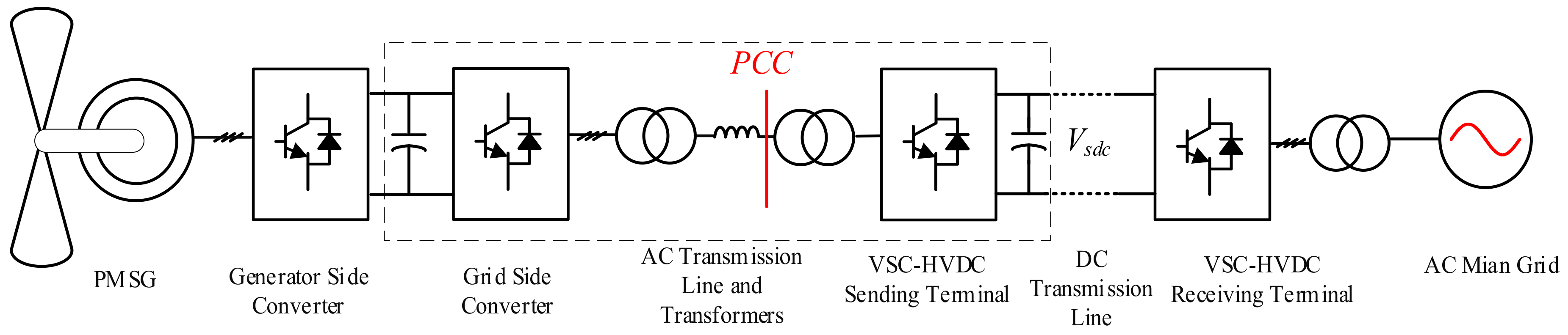
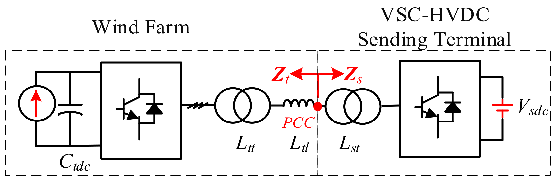
Figure 1 introduces a PMSG-based wind farm with a two terminal VSC-based HVDC system. The wind power grid side converter works as an AC current source, which is connected to the point of common coupling (PCC) through a transformer and AC transmission line. The HVDC sending terminal works as an AC voltage source to support the PCC. The HVDC receiving terminal is connected to the main power grid by a transformer. To simplify this system, the wind power generator side converters are considered as a DC current source, and a DC-link of HVDC is a constant DC voltage source. Consequently, for wind farms, only DC-link and grid side converters will be modelled. Meanwhile, the HVDC receiving terminal and the main power grid will be neglected in the following analysis.

2.2. VSC-HVDC Sending Terminal Control Bandwidths

Figure 2 shows the HVDC schematic circuit. The inductance, resistance and capacitance of the HVDC sending terminal converter LC filter are given by R_s, L_s and C_s, where the subscript ‘s’ denotes the HVDC sending terminal. The equivalent inductance of the transformer is given by L_st, and V_sdc represents the HVDC DC-link equivalent voltage. The valve voltage of the converter U_s is considered as an ideal controllable three-phase voltage source.

All models in this paper were built in a dq synchronization reference frame to correspond to the normal PI controller application in the converter. For a HVDC sending terminal, the d-axes aligned with the voltage vector e_s (the C_s voltage), and the q-axes leads the d-axes by π/2.

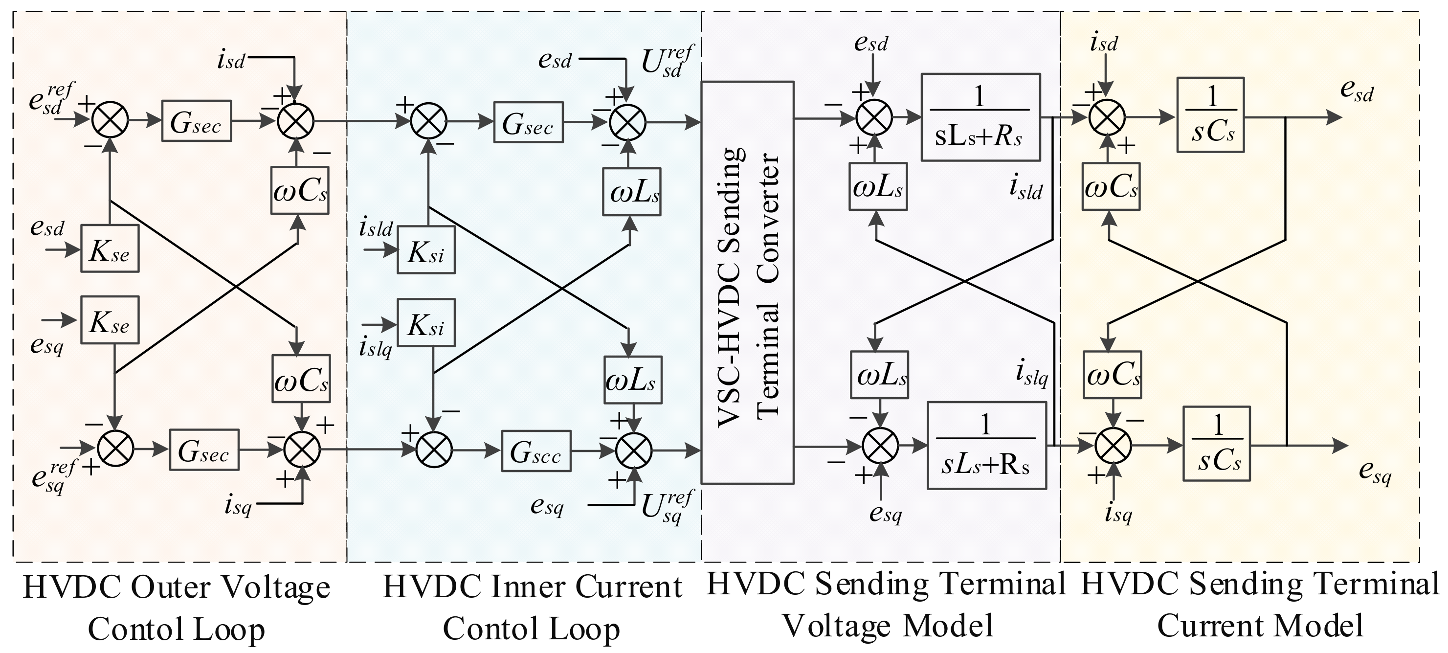
Figure 3 shows the dual-loop control loop schematic diagram of the HVDC sending terminal [22], where e_sd, e_sq, u_sd, u_sq are the C_s voltage and HVDC converter valve side voltages in the dq-frame, denoted by the subscript ‘d’ and ‘q’, respectively. The corresponding L_s currents are i_sLd and i_sLq.

A closed-current control loop C_scc is given in Equation (1), which describes the current dynamic performance in both the d and q-axes. The transfer function of the current controller is given by G_scc = k_spcc + k_sicc/s.

$$C_{scc}=\frac{s{k}_{spcc}+k_{sicc}}{s^2{L}_s+s\left(R_s+k_{spcc}\right)+k_{sicc}}$$

(1)

Equation (1) is modified to a first-order form by setting k_spcc = ω_sccL_s and k_sicc = ω_sccR_s as Equation (2), where ω_scc is the bandwidth of the closed current loop.

$$T_{scc}=\frac{{\omega }_{scc}}{s+{\omega }_{scc}}$$

(2)

A closed AC voltage control loop can be expressed as Equation (3), where G_sec = k_spec + k_siec/s is the AC voltage PI controller.

$$C_{sec}=\frac{s{k}_{spec}+k_{siec}}{s^2{C}_s+s{k}_{spec}+k_{siec}}$$

(3)

The closed-loop is written in a second-order form as Equation (4) by letting k_spec = 2ς_secω_snecC_s and k_siec = ${\omega }_{snec}^2$C_s, where ς_sec is the damping of the voltage control loop, and ω_snec is its natural frequency.

$$T_{sec}=\frac{2{\varsigma }_{sec}{\omega }_{snec}+{\omega }_{snec}^2}{s^2+2{\varsigma }_{sec}{\omega }_{snec}+{\omega }_{snec}^2}$$

(4)

Defining the AC voltage closed-loop bandwidth ω_sec when |T_sec| = 0.707, the relationship between the bandwidth ω_sec and the natural frequency ω_snec can be calculated using Equation (5).

$${\omega }_{snec}={\omega }_{sec}{\left({\left(4{\varsigma }_{sec}^4+4{\varsigma }_{sec}^2+2\right)}^{\frac{1}{2}}-2{\varsigma }_{sec}^2-1\right)}^2$$

(5)

2.3. VSC-HVDC Sending Terminal Impedance Modeling

To build the impedance model, the expression of a matrix form ΔU = ZΔI should be calculated [12], where Z is a 2 × 2 matrix impedance, and ΔU and ΔI are small signal voltage and current matrices of size 2 × 1 in the dq-frame. The bold letters represent matrix in this paper.

The VSC-HVDC sending terminal impedance in the dq-frame can be written as Z_s0, which is given as follows in Equation (6):

$$\begin{array}{ll}{Z}_{s0}=& {\left(\left(I-G_{sdel}\left(I-G_{scc}{G}_{sec}+G_{scc}{G}_{sdee}\right)\right)+\left(G_{sdel}\left(G_{sdec}-G_{scc}\right)+Z_{sL}\right)Y_{sc}\right)}^{-1}\\ & \left(G_{sdec}{G}_{sdel}+Z_{sL}\right)\end{array}$$

(6)

where

$$Z_{sL}=\left[\begin{array}{cc}s{L}_s+R_s& -\omega L_s\\ \omega L_s& s{L}_s+R_s\end{array}\right],Y_{sc}=\left[\begin{array}{cc}s{C}_s& -\omega C_s\\ \omega C_s& s{C}_s\end{array}\right],G_{sec}=-\left[\begin{array}{cc}{G}_{\sec }& 0\\ 0& G_{\sec }\end{array}\right]$$

$$G_{scc}=-\left[\begin{array}{cc}{G}_{scc}& 0\\ 0& G_{scc}\end{array}\right], G_{sdee}=-\left[\begin{array}{cc}0& -\omega C_s\\ \omega C_s& 0\end{array}\right],G_{sdec}=-\left[\begin{array}{cc}0& -\omega L_s\\ \omega L_s& 0\end{array}\right]$$

2.4. PMSG-Wind Converter Control Bandwidths

A type IV wind turbine with L filter connected to the PCC through a transformer and a cable is shown in Figure 4. An ideal converter model is used regardless of the PWM harmonic effect.

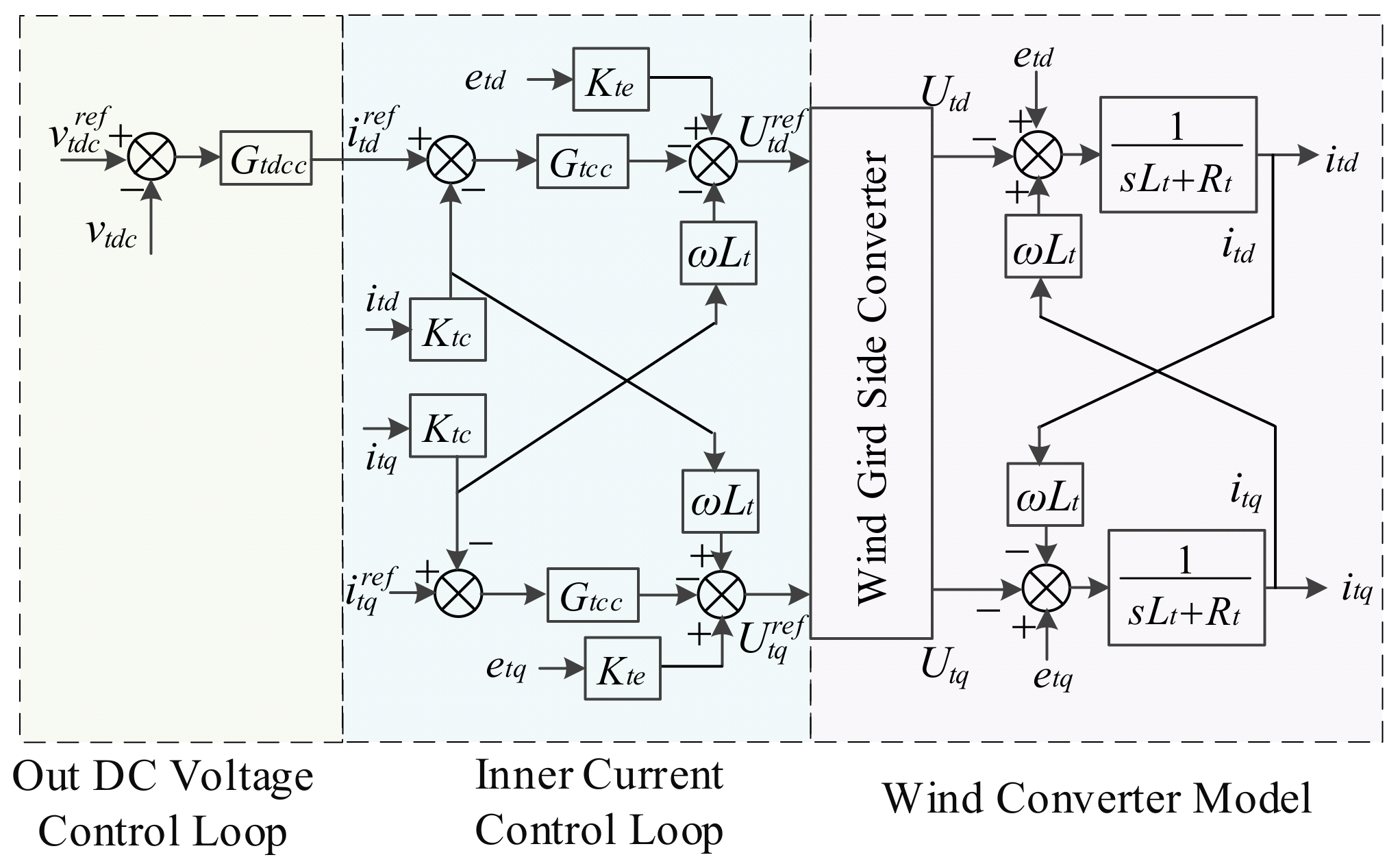
Figure 5 shows the outer DC-link voltage and inner current control loop schematic diagram of the grid side converter. The subscript ‘t’ stands for the wind turbine.

A current closed-loop in the d and q-axes can be obtained with Equation (7), where G_tcc = k_tpcc + k_ticc/s is the current PI controller, and L_t and R_t are the inductor and resistance of L filter, respectively.

$$C_{tcc}=\frac{s{k}_{tpcc}+k_{ticc}}{s^2{L}_t+s\left(R_t+k_{tpcc}\right)+k_{ticc}}$$

(7)

Equation (7) can be modified as a typical first-order transfer function as Equation (8) by k_tpcc = ω_tccL_t and k_ticc = ω_tccR_t, where ω_tcc is the bandwidth of the closed current loop.

$$T_{tcc}=\frac{{\omega }_{tcc}}{s+{\omega }_{tcc}}$$

(8)

The DC-link voltage closed-loop is given by Equation (9), where G_tdcc = k_tpdcc + k_tidcc/s is the DC-link voltage PI controller, and C_tdc is the DC-link capacitor. Setting k_tpdcc = 2ς_tdccω_tndccC_tdc and k_tidcc = ${\omega }_{tndcc}^2$C_tdc, Equation (9) can be modified as a typical second-order transfer function through Equation (10), where the damping ratio and natural frequency are given by ς_tdcc and ω_tndcc, respectively. Introducing the DC-link voltage closed loop bandwidth ${\omega }_{tdcc}$ which makes |T_tdcc| = 0.707, Equation (11) give the relationship between ω_tndcc and ω_tdcc.

$$C_{tdcc}=\frac{\frac{k_{tpdcc}}{C_{tdc}}s+\frac{k_{tidcc}}{C_{tdc}}}{s^2+\frac{k_{tpdcc}}{C_{tdc}}s+\frac{k_{tidcc}}{C_{tdc}}}$$

(9)

$$T_{tdcc}=\frac{2{\varsigma }_{tdcc}{\omega }_{tndcc}+{\omega }_{tdcc}^2}{s^2+2{\varsigma }_{tdcc}{\omega }_{tndcc}+{\omega }_{tndcc}^2}$$

(10)

$${\omega }_{tnecc}={\omega }_{tdcc}{\left({\left(4{\varsigma }_{tdcc}^4+4{\varsigma }_{tdcc}^2+2\right)}^{\frac{1}{2}}-2{\varsigma }_{tdcc}^2-1\right)}^2$$

(11)

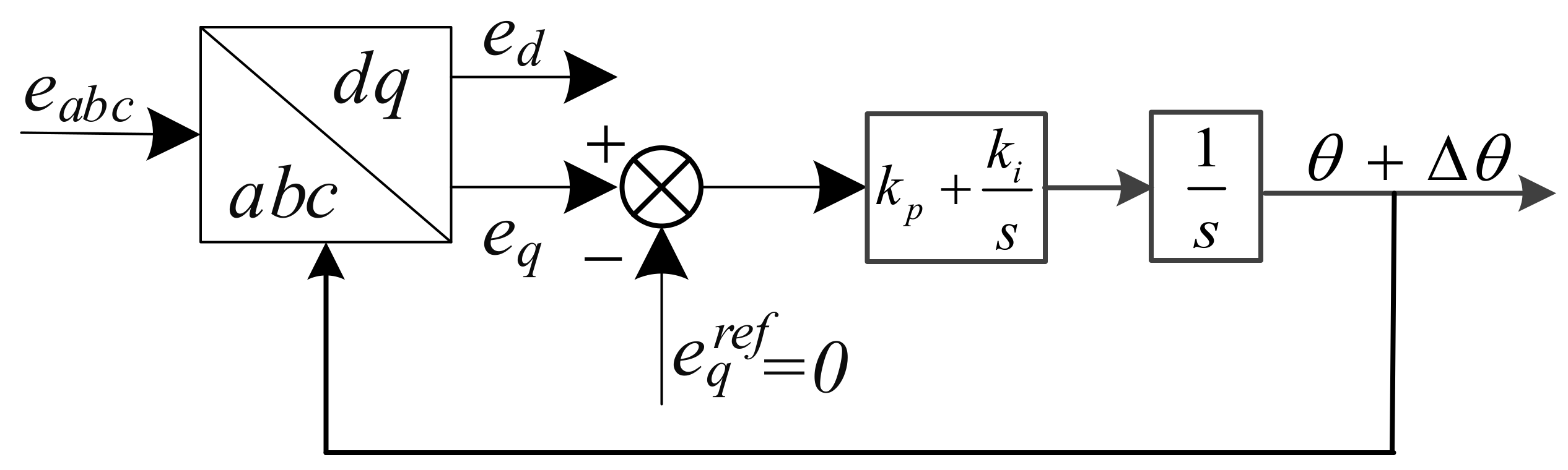
Figure 6 illustrates the block diagram of a common PLL, where the three-phase grid voltage e_abc is needed as the input, and the grid voltage phase θ is the output.

From paper [23], the closed PLL control loop is given as Equation (12), where G_tpllc = k_tppll + k_tipll/s is a PLL PI controller, and e_tx is the grid voltage without perturbation.

$$G_{tpll}=\frac{G_{tpllc}}{s+e_{tx}{G}_{tpllc}}$$

(12)

The closed PLL control loop can be re-expressed as T_tpll by setting k_tppll = 2ς_tpllcω_tnpll/e_td and k_tppll = ${\omega }_{tnpll}^2$/e_tx.

$$T_{tpll}=\frac{1}{e_{tx}}\frac{2{\varsigma }_{tpll}{\omega }_{tnpll}+{\omega }_{tnpll}^2}{s^2+2{\varsigma }_{tpll}{\omega }_{tnpll}+{\omega }_{tnpll}^2}$$

(13)

By defining the bandwidth when |T_tpll| = 0.707, the relationship between the PLL bandwidth and the natural frequency is shown by Equation (14).

$${\omega }_{tnpll}={\omega }_{tpll}{\left({\left(4{\varsigma }_{tpll}^4+4{\varsigma }_{tpll}^2+2\right)}^{\frac{1}{2}}-2{\varsigma }_{tpll}^2-1\right)}^2$$

(14)

2.5. PMSG-Wind Converter Impedance

Based on the outer DC-link voltage control loop and the inner current and PLL control loops, the impedance of the PMSG wind grid side converter can be derived from Equation (15); the detailed impedance-built process can be found in paper [24]. The subscript ‘x’ and ‘y’ stands for the system frame x-axes and y-axes, which are defined as the same as dq-frame when there is no perturbance in grid voltage. e_tx and e_ty and i_tx and i_ty are the grid side voltage and current in x-axes and y-axes.

$$\begin{array}{ll}{Z}_{t0}=& {\left(Z_{tL}-G_{tdel}\left(G_{tdec}-G_{tcc}-G_{tcc}{G}_{tdcc}{G}_{tdc}^i\right)\right)}^{-1}\\ & \left(I-G_{tdel}{G}_{tpll}^u{K}_{te}-G_{tel}{K}_{te}\left(G_{tpll}^e+G_{tdec}{G}_{tpll}^i-G_{tcc}{G}_{tpll}^i-G_{tcc}{G}_{tdcc}{G}_{tdc}^e\right)\right) \end{array}$$

(15)

where

$$\begin{gathered} Z_{tL}=\left[\begin{array}{cc}s{L}_t+R_t& -\omega L_t\\ \omega L_t& s{L}_t+R_t\end{array}\right],G_{tdc}^e=\frac{1}{s{C}_t{v}_{dc}}\left[\begin{array}{cc}{i}_{tx}& i_{ty}\\ 0& 0\end{array}\right], G_{tdc}^i=\frac{1}{s{C}_t{v}_{dc}}\left[\begin{array}{cc}{e}_{tx}& e_{ty}\\ 0& 0\end{array}\right] \\ {G}_{tpll}^e=\left[\begin{array}{cc}1& e_{ty}{G}_{tpll}\\ 0& 1-e_{tx}{G}_{tpll}\end{array}\right],G_{tpll}^i=\left[\begin{array}{cc}0& i_{ty}{G}_{tpll}\\ 0& -i_{tx}{G}_{tpll}\end{array}\right],G_{tpll}^u=\left[\begin{array}{cc}0& -u_{tq}{G}_{tpll}\\ 0& -u_{td}{G}_{tpll}\end{array}\right] \\ {G}_{tcc}=-\left[\begin{array}{cc}{G}_{tcc}& 0\\ 0& G_{tcc}\end{array}\right],G_{tdcc}=-\left[\begin{array}{cc}{G}_{tdcc}& 0\\ 0& 0\end{array}\right],G_{tdec}=-\left[\begin{array}{cc}0& -\omega L_t\\ \omega L_t& 0\end{array}\right] \end{gathered}$$

3. Impedance-Based System Stability Analysis

3.1. Basic Theory of the Impedance-Based System Stability Criterion

To employ the impedance stability criterion, the wind farm system with HVDC is divided into two interconnected parts by the PCC as shown in Figure 7. The impedance of the HVDC sending terminal is given by Z_s and its transformer impedance is Z_st. Meanwhile, Z_t contains the impedance of the remaining parts that include wind grid side converters, step up transformer’s impedance Z_tt and AC transmission line impedance Z_tl. The expressions Z_s and Z_t are given by Equations (16) and (17), respectively.

$$Z_s=N_{st}^2\left(Z_{s0}+Z_{st}\right)$$

(16)

$$Z_t=\frac{N_{tt}^2}{N_t^2}\left(Z_{t0}+Z_{tt}\right)+Z_{tl}$$

(17)

The transformer ratios of the HVDC and wind converter sides are given by N_st and N_tt, respectively. N_t is the number of grid-connected wind power grid side converters.

$$Z_{st}=\left[\begin{array}{cc}s{L}_{st}& -\omega L_{st}\\ \omega L_{st}& s{L}_{st}\end{array}\right], Z_{tt}=\left[\begin{array}{cc}s{L}_{tt}& -\omega L_{tt}\\ \omega L_{tt}& s{L}_{tt}\end{array}\right], Z_{tl}=\left[\begin{array}{cc}s{L}_{tl}& -\omega L_{tl}\\ \omega L_{tl}& s{L}_{tl}\end{array}\right]$$

Both Z_s and Z_t are size 2 × 2 matrices, and the GNC can be used for system stability analysis. The minor loop gain of the equal feedback control system is given as:

$$G(s)H(s)=\frac{Z_t}{Z_s}$$

which is also a 2 × 2 matrix. The minor loop gain matrix is defined as:

$$G(s)H(s)=\left[\begin{array}{cc}{Z}_{dd}& Z_{dq}\\ Z_{qd}& Z_{qq}\end{array}\right]$$

Generally, G(s)H(s) is asymptotically stable if and only if the characteristic loci for the eigenvalues of G(s)H(s), λ₁(s) and λ₂(s) taken together, do not encircle −1 for s = jω, and −∞ < ω < ∞ [21], where:

$${\lambda }_{1,2}(s)=\frac{Z_{dd}+Z_{qq}}{2}\pm \sqrt{{\left(\frac{Z_{dd}-Z_{qq}}{2}\right)}^2-Z_{dq}{Z}_{qd}}$$

If the off-diagonal elements Z_dq and Z_qd are relatively low in gain compared with the diagonal elements Z_dd and Z_qq, the eigenvalues of G(s)H(s) can be simplified to an approximate form with negligible impact on the system stability analysis [25,26].

$${\lambda }_{1,2}(s)=Z_{dd},Z_{qq}$$

Because the Bode plots of Z_dd and Z_qq correspond to their Nyquist plot, the Bode criterion has the same function as the GNC, which will be explained later. Furthermore, the bode criterion can be used to easily observe individual magnitude and phase stability tendency. Therefore, the Bode criterion is used as the main system stability criterion.

Additionally, before using the impedance stability criterion, the two parts from the PPC shown in Figure 7 should be individually stable. This requires the HVDC sending terminal to be stable when unloaded due to its voltage source working mode. Meanwhile, the wind power converter should be kept stable when connected to an ideal voltage source due to its current source working mode. All the cases in this study satisfied these two conditions.

3.2. Impedance Characters Analysis and Impact of Power Ratio on System Stability

To analyze the sub-/super-synchronous phenomenon by using the impedance criterion, detailed expression of Z_s and Z_t should be formulated. To apply the unity power factor control to wind power converters, the voltage and current in the q-axes are all considered to be equal to zero in the stable state. In addition, the wind grid side converter valve side voltage u_td and u_tq can be replaced by the grid voltage and current in the d-axes as u_td = e_td − R_ti_td and u_tq = −ωL_ti_td in the expression for the wind farm impedance in Equation (17). The off-diagonal elements in Equation (17) can also be neglected due to the unity power factor control [17,27,28]. Therefore, the minor loop gain can be simplified to an approximate form as λ₁(s) = Z_sdd/Z_tdd and λ₂(s) = Z_sqq/Z_tqq. The PWM delay and the voltage and current sample delays can also be neglected due to their small impact on the frequency band this paper is concerned with.

Based on the above conditions, the diagonal element expressions are given in Equations (18)–(20), where Z_sdd and Z_sqq represent HVDC sending terminal impedance on d and q-axes, respectively, Z_tdd and Z_tqq are the wind farm impedance in the d and q-axes, respectively.

$$Z_{sdd,sqq}=\frac{N_{st}^2\frac{G_{scc}{G}_{\sec }+(G_{scc}+s{L}_s+R_s)s{C}_s}{s{L}_s+R_s}}{{\left(\frac{G_{scc}{G}_{\sec }+(G_{scc}+s{L}_s+R_s)s{C}_s}{s{L}_s+R_s}\right)}^2+{\left(\omega C_s\right)}^2}+s{L}_{st}$$

(18)

$$Z_{tdd}=\frac{N_{tt}^2}{N_t}\left(\frac{s{L}_t+R_t+G_{tcc}}{G_{tcc}{G}_{tdcc}}\right)\frac{s{C}_{tdc}{v}_{tdc}}{i_{td}}-\frac{N_{tt}^2}{N_t}\frac{e_{td}}{i_{td}}+\frac{N_{tt}^2}{N_t}s{L}_{tt}+s{L}_{tl}$$

(19)

$$Z_{tqq}=\frac{N_{tt}^2}{N_t}\left(\frac{s{L}_t+R_t+G_{tcc}}{i_{td}{G}_{tcc}{G}_{tpll}}\right)+\frac{N_{tt}^2}{N_t}s{L}_{tt}+s{L}_{tl}$$

(20)

According to Equation (18), Z_sdd is equal to Z_sqq, because the HVDC sending terminal impedance does not contain coupling items and nonlinear parts such as PLL. Both Z_sdd and Z_sqq are independent of stable state points such as voltage and current. On the other hand, the inner current controller G_scc, outer AC voltage controller G_sec and LCL-filter parameters influence the HVDC impedance.

In contrast, according to Equations (19) and (20), the wind farm impedance Z_sdd and Z_sqq depend on stable state points such as e_td, i_td and v_tdc. Both Z_tdd and Z_tqq include the inner current controller G_tcc and L filter parameters. Moreover, the Z_tdd contains the DC voltage controller G_tdc because the DC voltage controller acts only on the d-axes, while Z_tqq has the PLL G_tpll for it acts only on the q-axes.

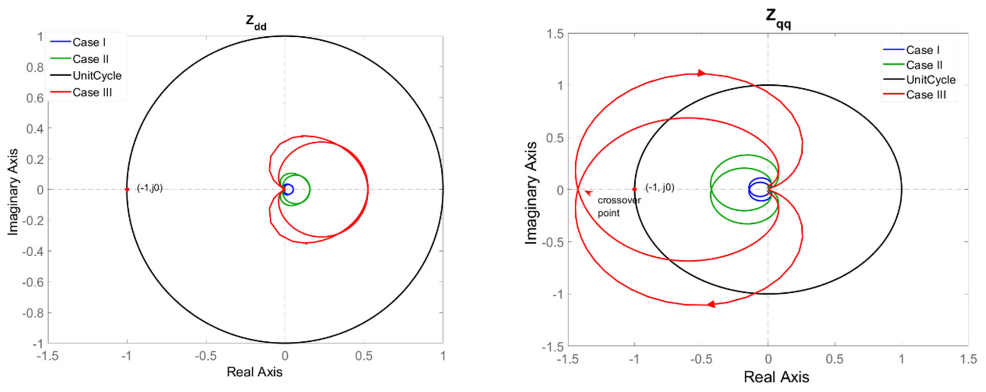
Figure 8 shows the Z_dd and Z_qq Nyquist plot of the HVDC and wind farm impedance interaction in increasing power ratios based on the system parameters in

Table 1. VSC-HVDC and equivalent wind farm system parameters.

Parameters	Value	Parameters	Value
Rated Power	100 MVA	Lt	0.2639 pu
Rated AC Voltage	160 kV	Rt	0.8402 pu
Rated Frequency	50 Hz	Ctdc	0.1486 pu
Ls	0.15 pu	vtdc	1.929 pu
Rs	0.0039 pu	Ltt	0.0123 pu
Cs	6.217 pu
Lst	0.057 pu

. Case I, Case II and Case III represent impedance based on a power ratio of 0.1 pu, 0.6 pu and 2 pu. For Z_dd, the three curves close in but are still far away from encircling the point (−1,j0), which means Z_dd is stable under these power ratios conditions. On the contrary, for Z_qq, the curves close in and finally in Case III the curve encircles the point (−1,j0) clockwise. Therefore, Z_qq is unstable under the highest power ratio. According to the GNC, the system is unstable if either Z_dd or Z_qq satisfies the instability criterion.

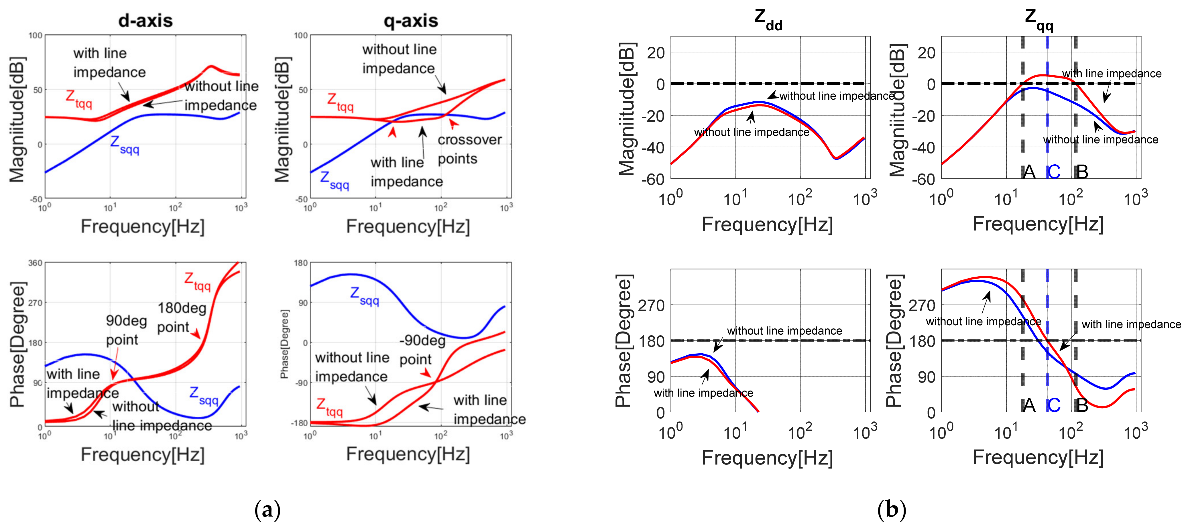
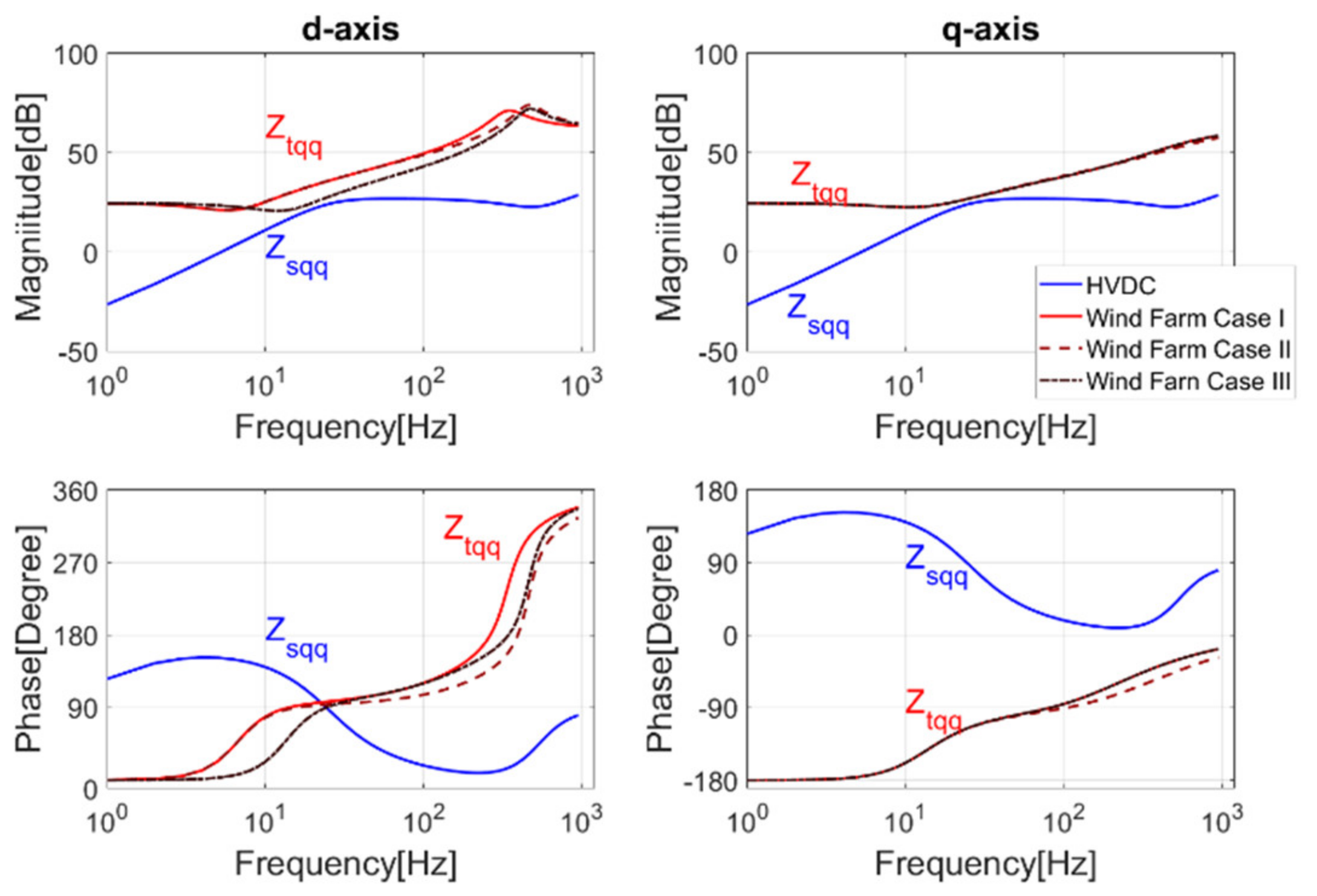
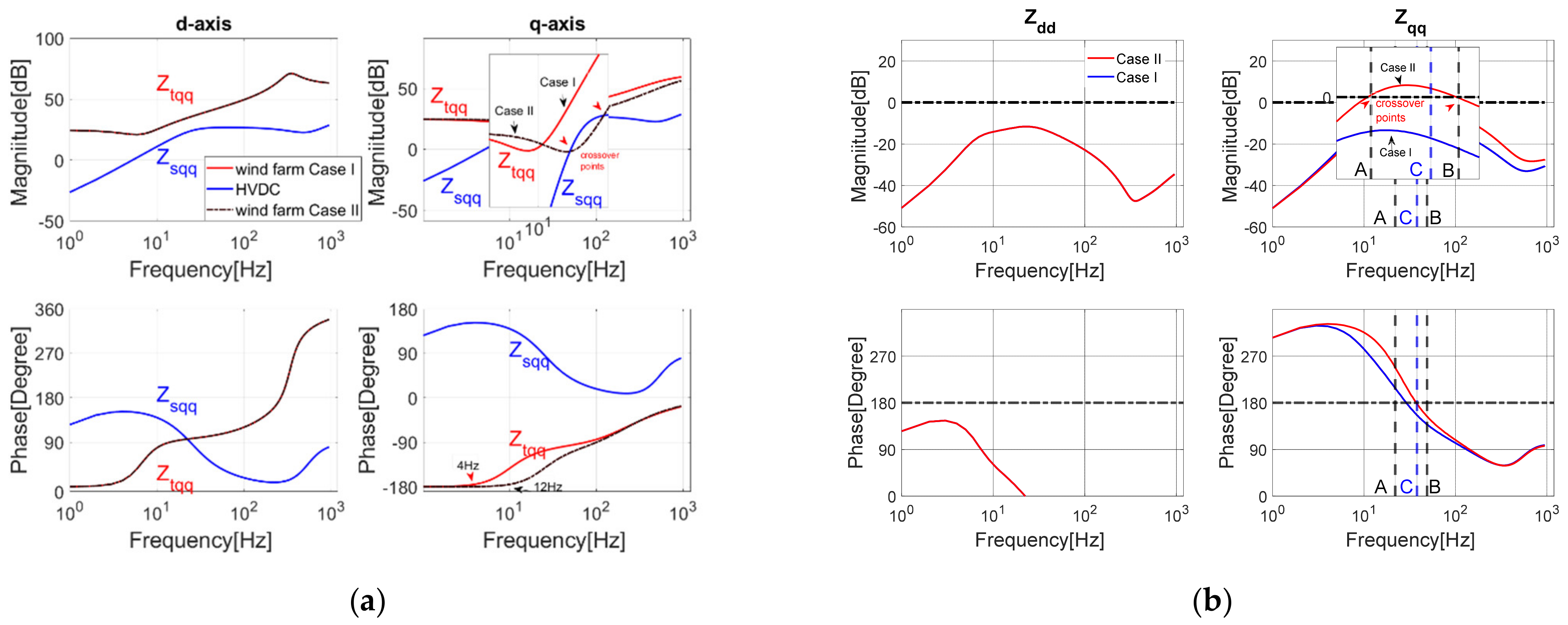
Figure 9a shows the corresponding Bode plots, which show that as the active current i_td increases, the HVDC impedance Z_sdd,sqq remains the same due to the independence of i_td. Meanwhile, the magnitude of wind farm impedance (Z_tdd and Z_tqq) decreases, as shown by the arrow. The Z_tqq in Case III reaches and crosses Z_sqq within 100 Hz. This tendency can be inferred by Equations (19) and (20), in which the active current i_td is the denominator of Z_tdd and Z_tqq.

The magnitude and phase change trends are demonstrated in the Bode plots of Z_dd and Z_qq in Figure 9b. The power ratios have small impact on the phases of Z_dd and Z_qq. The Z_dd phases cross at π on the frequency marked ‘C’. The Z_qq magnitudes for Cases I and II have no crossover at 0 dB. Case III goes up to 0 dB at frequency A and then down to 0 dB on frequency B. If the frequency C is between A and B, Z_qq is unstable for Case III. This is the application of the Bode criterion, which corresponds to encircling the point (−1,j0) in Figure 8. On the other hand, the magnitudes of Z_dd have no crossover point, which demonstrates their stability.

The above discussion shows that the crossover points of magnitude are necessary for system instability, which is also the key reason for the sub/sup-SCI between the HVDC and wind farm system. To increase system stability, it is reasonable to avoid the crossover points by increasing the magnitudes of Z_tdd and Z_tqq, and decreasing those of Z_sdd and Z_sqq in the low range frequency.

Based on Equations (19) and (20), the number of grid-connected wind grid side converters N_t has an impact on the magnitude of wind farm impedance that is similar to that of the power ratio. It is obvious that the worst-case scenario occurs when the whole wind farm delivers its rated power. The following analysis will be based on this extreme condition.

3.3. Impact of Line Impedance on System Stability

To analyze the line impedance impact on the system stability, Z_tdd and Z_tqq are studied without line impedance and with 100 mH line impedance.

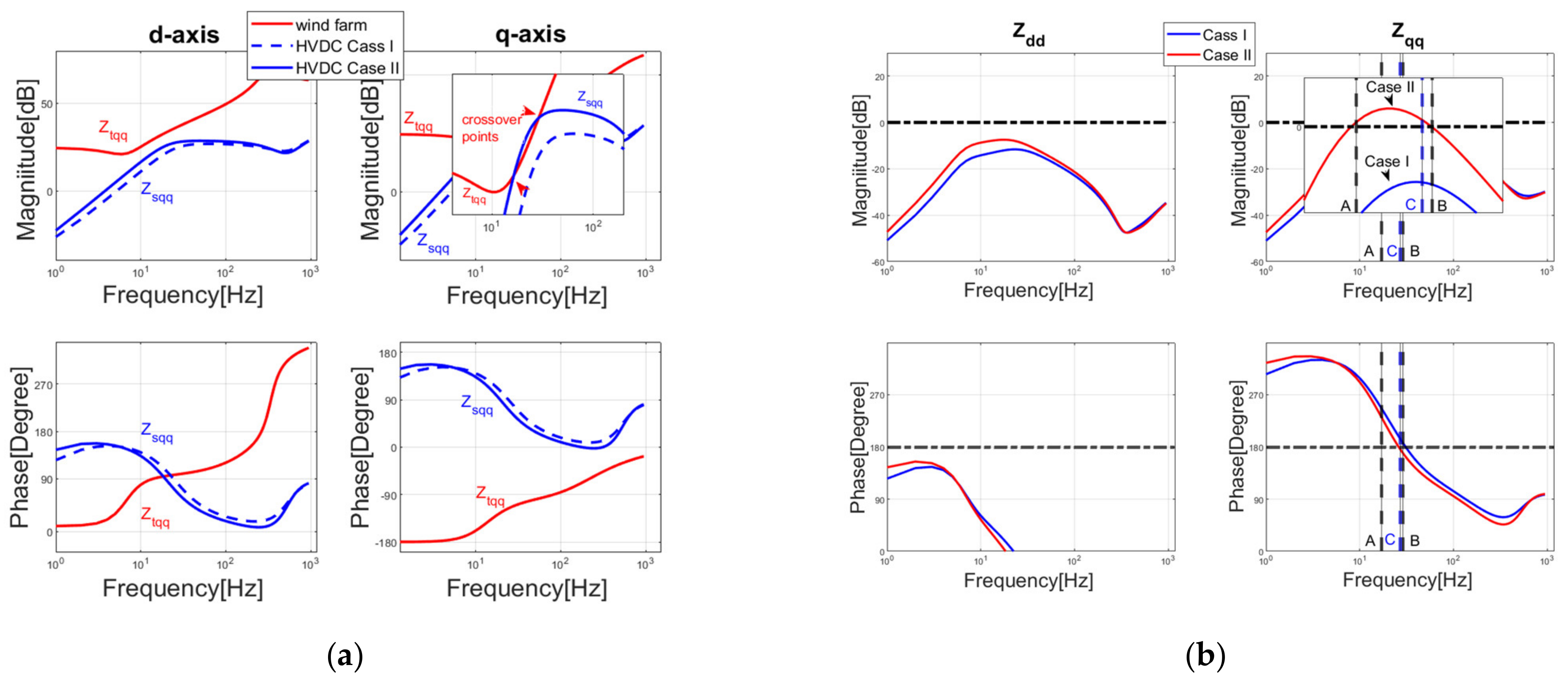
The HVDC and wind farm impedance interactions without and with line impedance are shown in Figure 10a. The phase part of Z_tdd shows that it is a positive resistive-inductive load for very low frequency range (between 0 Hz and about 30 Hz), as the phase is between 0 and 90 degrees. Between 30 Hz and about 310 Hz, the Z_tdd impedance is a negative resistive-inductive load, when its phase is between π/2 and π. This is the main phase characteristic of Z_tdd in the frequency domain.

As the inductive line impedance is added, the magnitudes of Z_tdd increase for frequencies between 0 Hz and around 310 Hz, as shown in Figure 10a. This increases the magnitude difference between the HVDC and wind farm on the d-axes and eliminates the possibilities of crossover. Based on the previous system stability analysis, the increased line impedance decreased the risk of Z_tdd instability.

On the contrary, the Z_tqq impedance has a negative resistive-capacitive load when the frequency is between 0 Hz and around 30 Hz, with its phase between −π and −π/2. The impedance turns to a positive resistive-capacitive load for frequencies between 30 Hz and more than 100 Hz. Consequently, the amplitude of Z_tqq decreases with the added line inductance impedance. This increased the possibility of HVDC and wind farm magnitude crossover points. Based on the previous system stability analysis, it can be stated that the line impedance increases the risk of Z_tqq instability. As the Bode plots of interactions in the q-axes show, with the 100 mH line impedance, the magnitude of wind farm has crossover points with the HVDC magnitude, which will lead to system stability.

Figure 10b shows the Bode plots of Z_dd and Z_qq considering line impedance. Z_dd magnitudes do not have crossover points with the 0 dB line, which indicates their stability. Meanwhile, the line impedance causes crossover points for Z_qq magnitude with 0 dB. With the phase conditions and based on the Bode criterion mentioned previously, Z_qq with line impedance is unstable. This proves theoretically that a certain line impedance can cause system instability.

3.4. Impact of Control Loop Bandwidths on Stability

According to the previous interpretation, the impedance models contain PI controllers, which are designed by considering control loop bandwidth and the damping ratio (set to 0.707). Therefore, it is more reasonable to investigate the relationship between system stability and control loop bandwidths, rather than the individual proportional or integral coefficients.

The controllers can be redefined as follows, by replacing the proportional and integral coefficients by their bandwidth for each PI controller in Equations (3)–(5), and (7)–(14) where the defined damping ratios are equal to 0.707.

$$G_{scc}={\omega }_{scc}\left(L_s+\frac{R_s}{s}\right), G_{sec}={\omega }_{sec}\left(0.6857C_s+{\omega }_{\sec }\frac{0.236C_s}{s}\right)$$

$$G_{tcc}={\omega }_{tcc}\left(L_t+\frac{R_t}{s}\right), G_{tdcc}={\omega }_{tdcc}\left(0.6857C_{tdc}+{\omega }_{tdcc}\frac{0.236C_{tdc}}{s}\right)$$

$$G_{tpll}=\frac{1}{e_{td}}\frac{\left(0.6857{\omega }_{tpll}s+0.236{\omega }_{tdcc}^2\right)}{s^2+0.6857{\omega }_{tpll}s+0.236{\omega }_{tdcc}^2}$$

It is more specific to study the impact of bandwidth on stability by inserting these controllers into Equations (18)–(20) and obtaining Equations (21)–(23) below:

$$Z_{sdd,sqq}=N_{st}^2\frac{{\omega }_{scc}{\omega }_{sec}\left(0.6857+{\omega }_{\sec }\frac{0.236}{s}\right)+(s{\omega }_{scc}+1)}{s{C}_s{\left({\omega }_{scc}{\omega }_{sec}\left(0.6857+{\omega }_{\sec }\frac{0.236}{s}\right)+(s{\omega }_{scc}+1)\right)}^2+{\left(\omega C_s\right)}^2}+s{L}_{st}$$

(21)

$$Z_{tdd}=\frac{N_{tt}^2}{N_t}\left(\frac{\frac{s}{{\omega }_{tcc}}+1}{\left(0.6857+{\omega }_{tdcc}\frac{0.236}{s}\right)}\right)\frac{s{v}_{tdc}}{i_{td}}-\frac{N_{tt}^2}{N_t}\frac{e_{td}}{i_{td}}+\frac{N_{tt}^2}{N_t}s{L}_{tt}+s{L}_{tl}$$

(22)

$$Z_{tqq}=\frac{N_{tt}^2}{N_t}\left(\frac{\frac{s}{{\omega }_{tcc}}+1}{\frac{0.6857{\omega }_{tpll}s+0.236{\omega }_{tdcc}^2}{s^2+0.6857{\omega }_{tpll}s+0.236{\omega }_{tdcc}^2}}\right)\frac{e_{td}}{i_{td}}+\frac{N_{tt}^2}{N_t}s{L}_{tt}+s{L}_{tl}$$

(23)

3.4.1. Impact of HVDC Controller Loop Bandwidths

Due to the inner and outer control loops design principle, the bandwidth of the inner current control loop should be set as 10 times that of the outer AC voltage control loop. Therefore, it is logical to keep the relationship between the two bandwidths fixed when discussing the impact of bandwidths on impedance.

From Equation (21), it is clear that the highest orders of the current control loop bandwidth ω_scc and the AC voltage control loop bandwidth ω_sec in the denominator are two and four, respectively, which are double those in their respective numerators. This signifies that the reduction in ω_scc and ω_sec will increase Bode plots magnitudes, which raises the stability risk.

Figure 11a shows the Z_tdd and Z_tqq Bode plots under different bandwidths in proportional change. In the presence of the wind farm impedance, the current bandwidth is reduced from 10 pu (500 Hz) (Case I) to 9 pu (450 Hz) (Case II), while the outer AC voltage control loop bandwidth is reduced from 1 pu (50 Hz) (Case I) to 0.9 pu (45 Hz) (Case II), and the magnitude of Z_tqq rose and crosses the wind farm impedance.

In Figure 11b, the Bode plots of Z_dd and Z_qq can show this variation from a stable to unstable condition. The magnitude of Case I in the q-axes has no crossover points with the 0 dB line. The magnitude of Case II in the q-axes has a crossover up to the 0 dB line before its phase crosses down to the π line, and subsequently crosses back down to 0 dB after the phase crosses down to π. This indicates that Z_qq changes from stable to unstable when the bandwidths change. Although the magnitude of Z_dd also increases, it is too small and the phase of Z_dd will not affect the system stability.

3.4.2. Impact of Wind Grid Side Controller Loop Bandwidths

According to Z_tdd in Equation (22), ω_tdcc exists only in the denominator. Therefore, the bandwidths and Z_tdd magnitude are inversely proportional. It can be observed from Equations (22) and (23), that ω_tcc exists in the form of s/ω_tcc + 1 the in numerators of both equations. Due to its relatively higher value compared to 1, ω_tcc has a small impact on the magnitudes of Z_tdd and Z_tqq.

Figure 12 compares Z_tdd and Z_tqq for different values of ω_tcc and ω_tdcc. Firstly, only ω_tcc increases from 4 pu (200 Hz) (Case I) to 8 pu (400 Hz) (Case II), while the ω_tdcc is fixed at 0.8 pu (40 Hz). These two cases show little impact on either Z_tdd or Z_tqq in magnitude or phase. Secondly, in Case III, ω_tdcc changes from 0.4 pu (20 Hz) (Case I) up to 0.8 pu (40 Hz), while ω_tcc is kept fixed at 4 pu (200 Hz). The magnitude of Z_tdd decreases while that of Z_tqq remains stable. The lowest magnitude points of Z_tdd move closer to those of Z_sdd, which indicates the rising risk of instability, but considering the phase conditions, it is hard for Z_tdd to lead to system instability.

It can be observed from Equation (23) that the ω_tpll is part of Z_tqq denominator in a form of second-order function. Therefore, when the ω_tpll increases, the Z_tqq magnitude in the increased bandwidth area will decrease rapidly and rest frequency areas almost remain the same.

Figure 13a shows the Z_tqq with ω_tpll from 20 Hz (Case I) to 50 Hz (Case II). The magnitude falls to have crossover with Z_sqq. The range of phase near −π are extended from 4 to 12 Hz, which increased the possibility of phase instability. However, because ω_tpll has no impacts on Z_sdd as mentioned before, Z_sdd remains the same.

Figure 13b is the Bode plot of Z_qq and shows that Z_qq becomes unstable from an originally stable condition.

3.5. Impacts of Wind Grid Side Converter Switching Frequency

Considering the switching losses and limitations of the switching devices, the switching frequency for a wind power converter is in the range of 1–2 kHz. This limits its bandwidths, such as ω_dcc, ω_tcc, and ω_tpll. Developments in power switching devices, such as SiC and the multilevel topology application, have enabled the wind grid side converters to have a higher switching frequency, such as 3 kHz and more. Consequently, wider bandwidths are allowed, especially for ω_tpll. Therefore, the higher switching frequency may have the same impact on system stability as the increased ω_tpll.

4. Simulation Results and Stability Improvement by Bandwidth Modification

In this section, case studies will be presented to verify the previous conclusions by Matlab/Simulation. Subsequently, stability improvements by means of modifying the bandwidths will be proposed.

Table 2. VSC-HVDC and equivalent wind farm system control bandwidths.

Parameters	Value	Parameters	Value
ωscc	7 pu	ωtcc	6 pu
ωsec	0.7 pu	ωtdcc	0.6 pu
		ωtpll	0.9 pu

shows the VSC-HVDC and equivalent wind farm control bandwidths for a stable system.

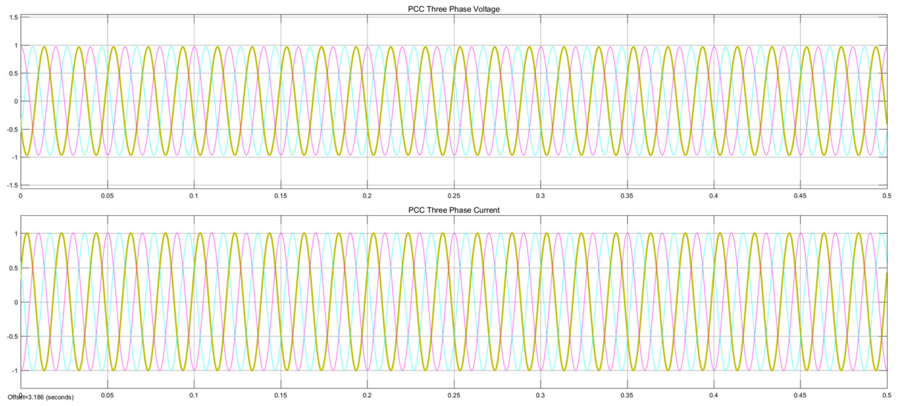
Figure 14 shows the PCC phase voltage and current in the abc-frame under free line impedance, and

Table 3. FFT spectra of PCC voltage and current under stable condition.

	PCC Voltage	Value (50 Hz Based pu)	PCC Current	Value (50 Hz Based pu)
FFT Spectrum	50 Hz (based frequency)	1	50 Hz (based frequency)	1

shows their FFT spectra. This figure and table show that the system only contains voltage and current at a frequency of 50 Hz. Therefore, the system operates in a stable condition.

4.1. Simulations on the Line Impedance Impact

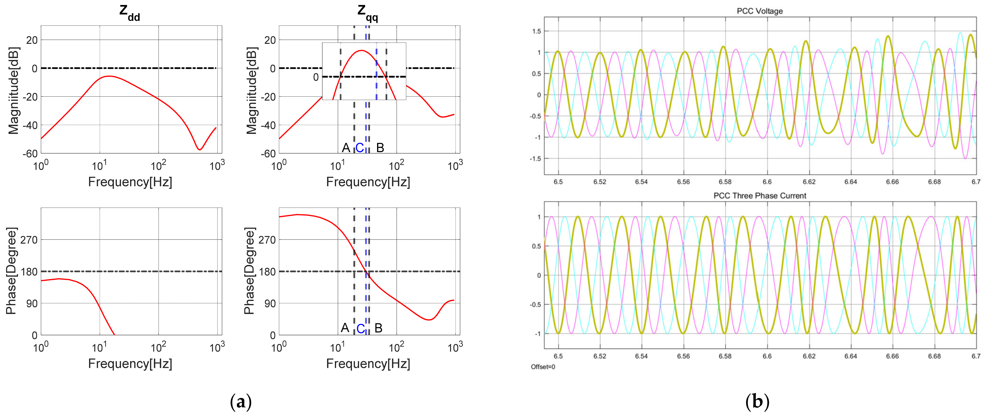
Figure 15a shows the Bode plots of Z_dd and Z_qq when the line impedance is 100 mH. The plot of Z_qq shows that the system becomes unstable. Figure 15b shows the PCC instantaneous voltage and current, and

Table 4. FFT spectra of voltage and current under unstable conditions caused by line impedance.

	PCC Voltage	Value (50 Hz Based pu)	PCC Current	Value (50 Hz Based pu)
	50 Hz (base frequency)	1	50 Hz (base frequency)	1
	8 Hz	0.05	8 Hz	0.07
FFT Spectrum	21 Hz	0.22	21 Hz	0.35
	79 Hz	0.43	79 Hz	0.36
	108 Hz	0.05	108 Hz	0.04

shows their FFT spectra. Both the voltages and currents have low frequency oscillations at around 8 Hz, 108 Hz, 21 Hz and 79 Hz. This proves that line impedance can lead to system instability.

4.2. Simulation on the Bandwidths Impact

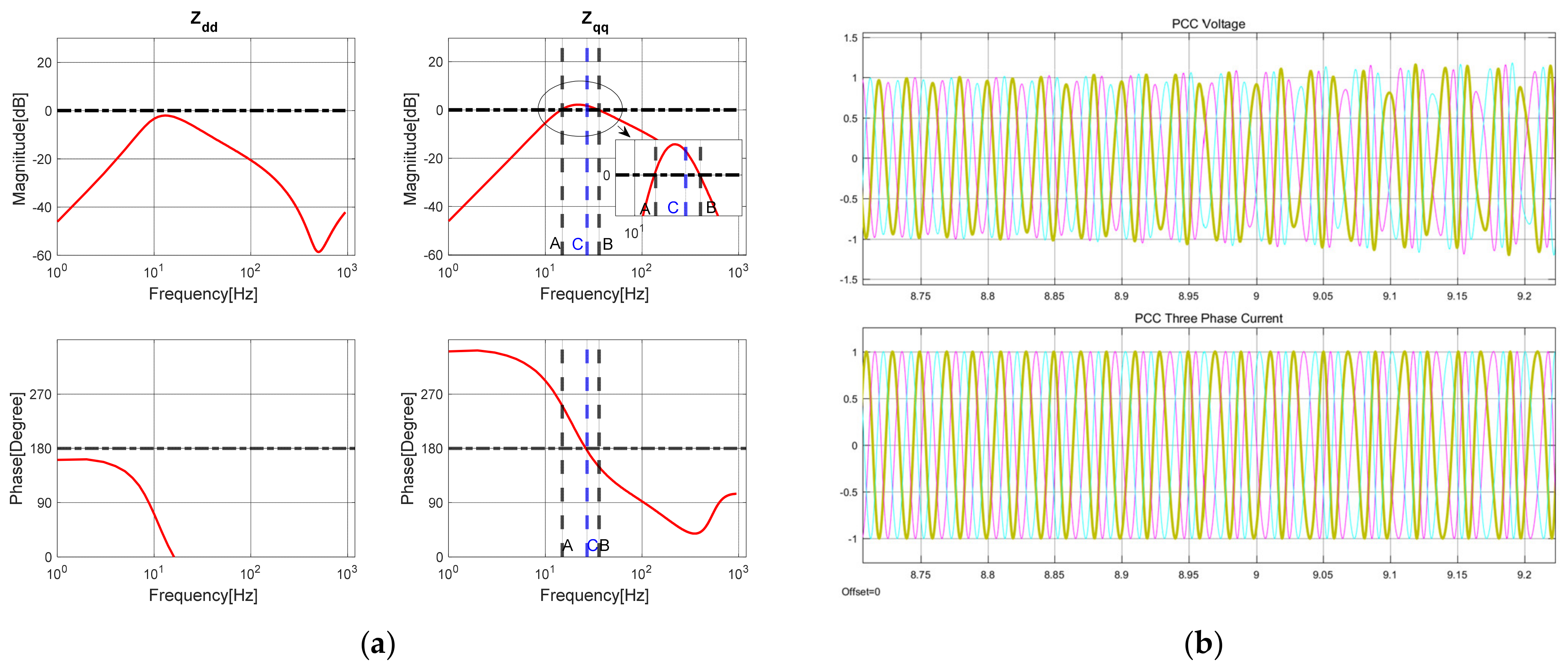
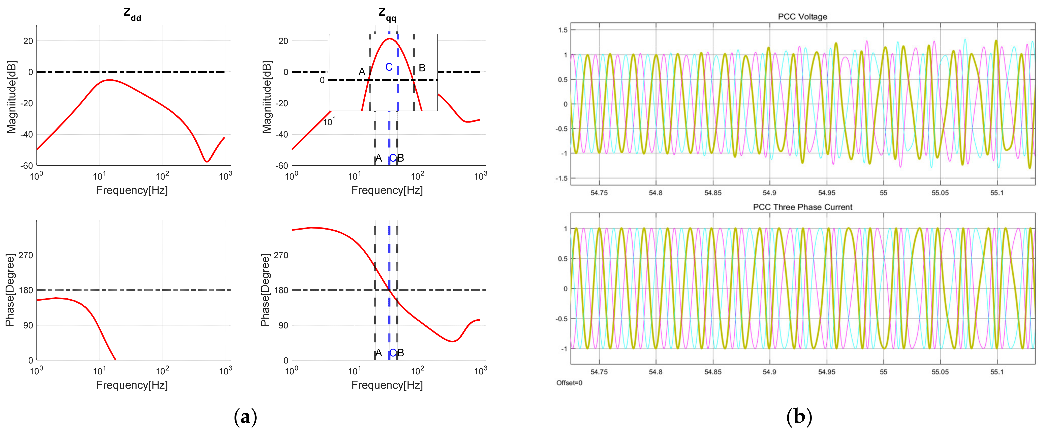
Figure 16a shows the Bode plots of Z_dd and Z_qq where ω_scc and ω_sec are 6 pu (300 Hz) and 0.6 pu (30 Hz), respectively, which are reduced from the original 7 pu (350 Hz) and 0.7 pu (35 Hz), respectively. It shows that the system becomes unstable in Z_qq. The unstable simulation results of the three phases’ voltage and current and their FFT spectra are provided in Figure 16b and

Table 5. FFT spectra of voltage and current under unstable conditions caused by decreased HVDC bandwidths.

	PCC Voltage	Value (50 Hz Based pu)	PCC Current	Value (50 Hz Based pu)
	50 Hz (base frequency)	1	50 Hz (base frequency)	1
	1 Hz	0.12	1 Hz	0.18
FFT Spectrum	24.5 Hz	0.40	24.5 Hz	0.58
	75.5 Hz	0.55	75.5 Hz	0.59
	101 Hz	0.11	101 Hz	0.17

, respectively. The table shows that the oscillation frequency is around 24.5 and 75.5 Hz, respectively. Compared with the three phases’ voltage and current in Figure 14, the reductions in ω_scc and ω_sec are the reasons for this system instability.

Figure 17a shows the Bode plots of Z_dd and Z_qq when the ω_tpll changes from 45 Hz to 68 Hz. The Z_qq is unstable according to the Bode criterion. Figure 17b shows its three-phase voltage and current, in which the oscillation occurs.

Table 6. FFT spectra of voltage and current under unstable conditions caused by increased wind farm PLL bandwidth.

	PCC Voltage	Value (50 Hz Based pu)	PCC Current	Value (50 Hz Based pu)
	50 Hz (based frequency)	1	50 Hz (based frequency)	1
FFT Spectrum	15 Hz	0.29	15 Hz	0.44
	85 Hz	0.38	85 Hz	0.43

shows that the voltage and current oscillation frequencies are about 15 Hz and 85 Hz. The increased ω_tpll could cause the system to become unstable.

To validate the previous analysis about the inner current and outer DC voltage control loop bandwidth impact, simulations that double the bandwidths ω_tcc and ω_tdcc from the original 300 Hz and 30 Hz to 600 Hz and 60 Hz were carried out. The system is still stable, the three-phase voltage and current similar to those in Figure 14. This shows these two bandwidths have little impact on system stability as indicated by the previous study.

4.3. Stability Improvement by Bandwidth Modification

The simulations shown earlier serve as proof of the previous theoretical study. Based on this, there are two ways to improve the system stability by bandwidth modification: (1) reduce the ω_tpll of wind grid side converters; (2) enlarge the HVDC bandwidths.

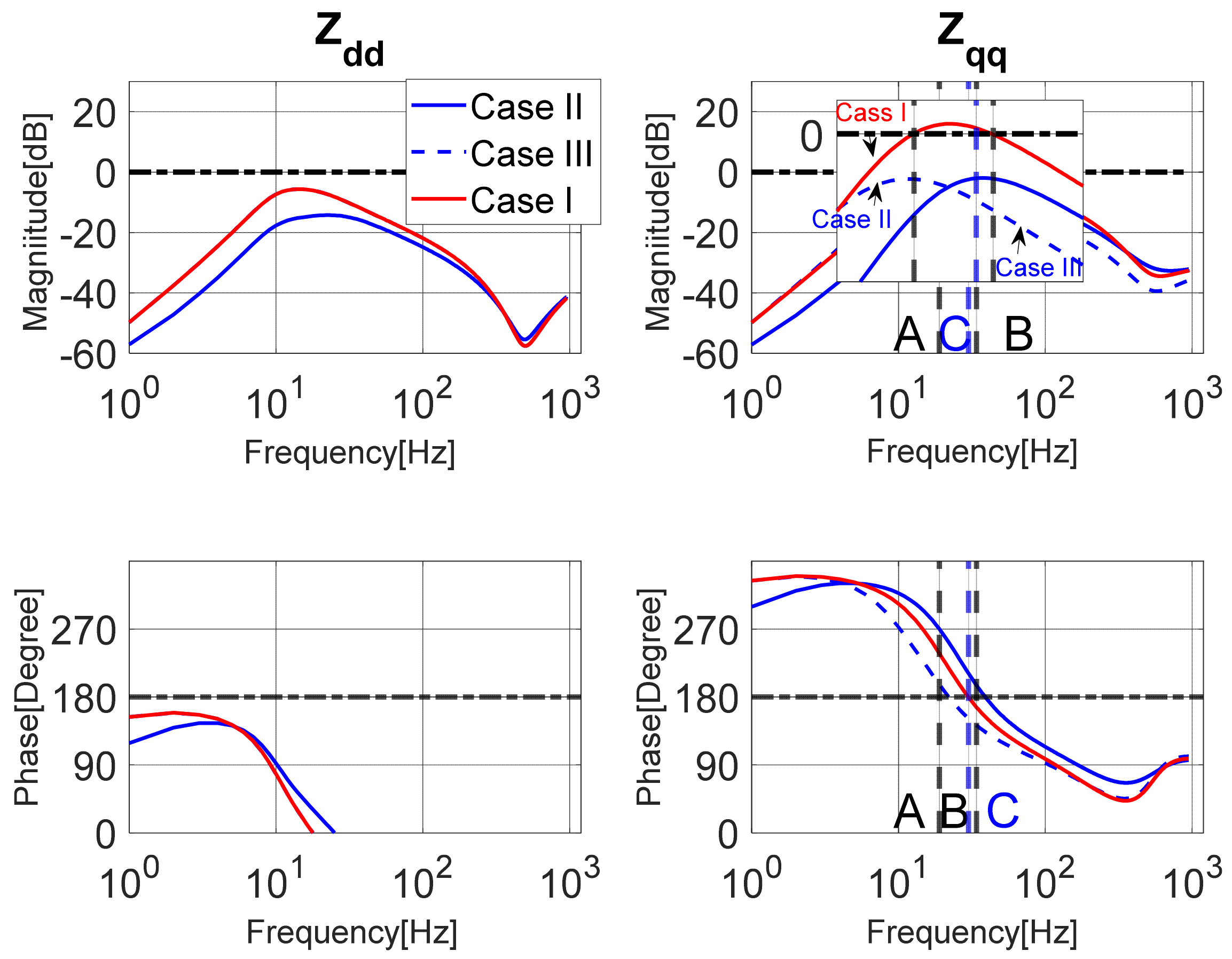
The following simulations compare two methods of system stability improvement by bandwidth modification. Figure 18 shows the Bode plots of Z_dd and Z_qq for three cases. Case I is the unstable system, which is the same as that shown in Figure 14 with 150 mH line impedance. Case II reduces the ω_tpll from the original 0.9 pu (45 Hz) to 0.4 pu (20 Hz), while Case III extends the ω_scc and ω_sec from the original 7 pu (350 Hz) and 0.7 pu (35 Hz) to 10.7 pu (535 Hz) and 1.07 pu (53.5 Hz).

The magnitude of Z_qq in Case I has crossover points with 0 dB, which is the key condition causing instability. Previous simulation has ready shown its unstable result. Both Cases II and III reduce the magnitude of Z_qq, which avoids the crossover points. In Cases II and III the system become stable by the Bode criterion. Simulations validate the impact of bandwidth modification methods.

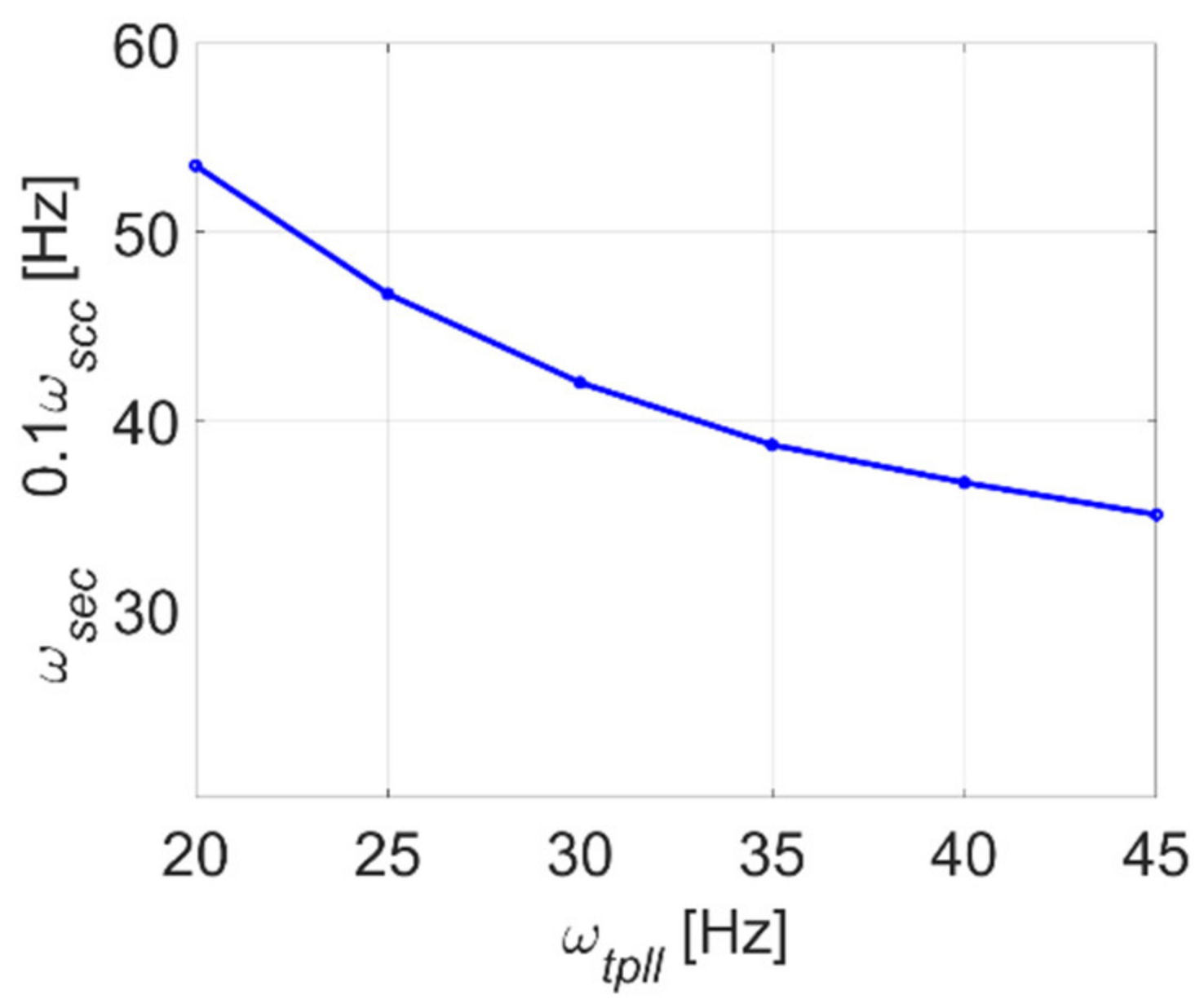
Based on the observation that in Cases II and III that the magnitude reaches Z_qq the same level, it can be gathered that the changes in ω_scc, ω_sec and ω_tpll have an equivalent function. Therefore, the relationship between ω_scc, ω_sec and ω_tpll can be found to have a similar impact on Z_qq magnitude within a certain range. In Figure 19, the original point is (45, 35), which means ω_tpll = 45 Hz and ω_sec = 0.1ω_see = 35 Hz. The point (40, 36.7) in the curve in Figure 19 signified that a 5 Hz reduction in ω_tpll and a 1.7 Hz increment in ω_sec (a 17 Hz increment of ω_scc) can reduce the Z_qq magnitude to the same degree. Based on this figure, it can be concluded that generally the Z_qq magnitude is more sensitive to ω_sec (ω_scc) than ω_tpll within certain a bandwidth range.

However, the LVRT and HVRT require the wind grid side converters to have a fast response, which needs the ω_tpll to be set to a high value. Meanwhile, the HVDC needs to limit its bandwidths to take into consideration the possible disturbance. Consequently, the ability to enhance the system stability by bandwidth modification is effective but has limited utility.

By techno-economic and risk analysis (TERA), bandwidths’ modification to enhance the system stability is an economical method compared with using oscillation suppression devices. The economic losses in sub/sup-synchronous interaction events are also significant. Between only September 2015 and September 2016, there were over 111 cases recorded in China. Each time the lost wind power was at least 50 MW; sometimes it could be up to 300 MW. The approved sub/sup-synchronous interaction depression method application is expected to avoid these losses with minor expense.

5. Discussion and Conclusions

This paper presented an analysis of sub/super-SCI in a VSC-HVDC and PMSG-based wind farm system with AC transmission line. After simplifying the impedance equations, a Bode criterion for system stability was used, which showed the unstable magnitude and phase conditions more clearly than the GNC. The wind farm impedance phase on the q-axes easily satisfied the instability condition due to the negative resistive-capacitive chrematistics. Therefore, the q-axes magnitude crossover points between the wind farm and HVDC were essential for system stability. The mathematical relations between the impedance magnitude and elements were demonstrated explicitly according to the detailed impedance expression. The results suggested that increasing the power ratio and line impedance helped form the crossover point by reducing the wind farm q-axes impedance magnitude. It was also discovered that the reduction in the HVDC and extension of the wind farm PLL control loop bandwidths affected the system stability in a similar manner. The outer DC voltage control loop bandwidth and inner current control loop of the wind converters had a negligible impact on q-axes magnitude and phase.

It is possible to improve system stability by reducing the PLL bandwidth and extending the bandwidths of HVDC, and simulation results supported this analysis. However, the limitations of this improvement approach were also discussed. It was found that the magnitude was more sensitive to HVDC bandwidth than that of the PLL; therefore, it was better to modify the HVDC bandwidth. Thus, the stability was optimized to a certain degree by bandwidth adjustments.

Compared with the oscillation suppression device installations, the approach this paper provided, which offered guidance to redesign the relevant controllers’ bandwidths, was easy to access in application in a low-cost way. However, this method only increased the magnitude margin of Z_qq. The unstable phase condition of Z_qq was hard to change. As a consequence, accurate parameters for impedance models were required and robustness of this approach was reduced.

References

- Mahela, O.P.; Gupta, N.; Khosravy, M.; Patel, N. Comprehensive Overview of Low Voltage Ride through Methods of Grid Integrated Wind Generator. IEEE Access 2019, 7, 99299–99326. [Google Scholar] [CrossRef]
- Dos Santos, M.L.; Jardini, J.A.; Casolari, R.P.; Vasquez-Arnez, R.L.; Saiki, G.Y.; Sousa, T.; Nicola, G.L.C. Power Transmission Over Long Distances: Economic Comparison Between HVDC and Half-Wavelength Line. IEEE Trans. Power Deliv. 2014, 29, 502–509. [Google Scholar] [CrossRef]
- Li, R.; Yu, L.; Xu, L.; Adam, G.P. Coordinated Control of Parallel DR-HVDC and MMC-HVDC Systems for Offshore Wind Energy Transmission. IEEE J. Emerg. Sel. Top. Power Electron. 2020, 8, 2572–2582. [Google Scholar] [CrossRef]
- Flourentzou, N.; Agelidis, V.G.; Demetriades, G.D. VSC-Based HVDC Power Transmission Systems: An Overview. IEEE Trans. Power Electron. 2009, 24, 592–602. [Google Scholar] [CrossRef]
- Wang, Y.; Zhao, C.; Guo, C.; Rehman, A.U. Dynamics and Small Signal Stability Analysis of PMSG-Based Wind Farm with an MMC-HVDC System. CSEE J. Power Energy Syst. 2020, 6, 226–235. [Google Scholar]
- Wang, Y.; Wang, L.; Jiang, Q. Impact of Synchronous Condenser on Sub/Super-Synchronous Oscillations in Wind Farms. IEEE Trans. Power Deliv. 2020, 36, 2075–2084. [Google Scholar] [CrossRef]
- Ebrahimzadeh, E.; Blaabjerg, F.; Wang, X.; Bak, C.L. Reducing Harmonic Instability and Resonance Problems in PMSG-Based Wind Farms. IEEE J. Emerg. Sel. Top. Power Electron. 2018, 6, 73–83. [Google Scholar] [CrossRef]
- Adams, J.; Carter, C.; Huang, S.-H. ERCOT Experience with sub-synchronous control interaction and proposed remediation. In Proceedings of the PES T D 2012, Orlando, FL, USA, 7–10 May 2012; pp. 1–5. [Google Scholar]
- Wang, L.; Xie, X.; Jiang, Q.; Liu, H.; Li, Y.; Liu, H. Investigation of SSR in Practical DFIG-Based Wind Farms Connected to a Series-Compensated Power System. IEEE Trans. Power Syst. 2015, 30, 2772–2779. [Google Scholar] [CrossRef]
- Sun, K.; Yao, W.; Fang, J.; Ai, X.; Wen, J.; Cheng, S. Impedance Modeling and Stability Analysis of Grid-Connected DFIG-Based Wind Farm With a VSC-HVDC. IEEE J. Emerg. Sel. Top. Power Electron. 2020, 8, 1375–1390. [Google Scholar] [CrossRef]
- Zhu, L.; Zhong, D.; Wang, B.; Lin, R.; Xu, M. Understanding Subsynchronous Oscillation in DFIG-Based Wind Farms with Rotor-Side Converter Control Based on the Equivalent RLC Model. IEEE Access 2020, 8, 65371–65382. [Google Scholar] [CrossRef]
- Lv, J.; Dong, P.; Shi, G.; Cai, X.; Rao, H.; Chen, J. Subsynchronous oscillation of large DFIG-based wind farms integration through MMC-Based HVDC. In Proceedings of the 2014 International Conference on Power System Technology, Chengdu, China, 20–22 October 2014; pp. 2401–2408. [Google Scholar]
- Lv, J.; Dong, P.; Shi, G.; Cai, X.; Li, X. Subsynchronous Oscillation and Its Mitigation of MMC-Based HVDC with Large Doubly-Fed Induction Generator-Based Wind Farm Integration. Proc. CSEE 2015, 35, 4852–4860. [Google Scholar]
- Hanchao, L.; Jian, S. Voltage Stability and Control of Offshore Wind Farms with AC Collection and HVDC Transmission. IEEE J. Emerg. Sel. Top. Power Electron. 2014, 2, 1181–1189. [Google Scholar] [CrossRef]
- Sowa, I.; Domínguez-García, J.L.; Gomis-Bellmunt, O. Impedance-Based Analysis of Harmonic Resonances in HVDC Connected Offshore Wind Power Plants. Electr. Power Syst. Res. 2019, 166, 61–72. [Google Scholar] [CrossRef]
- Lv, J.; Cai, X.; Zhang, Z.; Chi, Y. Impedance Modeling and Stability Analysis of MMC-based HVDC for Offshore Wind Farms. Proc. CSEE 2016, 36, 3771–3781. [Google Scholar]
- Amin, M.; Molinas, M. Understanding the Origin of Oscillatory Phenomena Observed Between Wind Farms and HVdc Systems. IEEE J. Emerg. Sel. Top. Power Electron. 2017, 5, 378–392. [Google Scholar] [CrossRef] [Green Version]
- Xie, X.; Liu, H.; He, J.; Zhang, C.; Qiao, Y. Mechanism and Characteristics of Subsynchronous Oscillation Caused by the Interaction between Full-converter Wind Turbines and AC Systems. Proc. CSEE 2016, 36, 2366–2372. [Google Scholar]
- Lv, J.; Cai, X. Controller Parameters Optimization Design for Enhancing the Stability of Wind Farm With VSC-HVDC System. Proc. CSEE 2018, 38, 431–434. [Google Scholar]
- Amin, M.; Molinas, M.; Lyu, J. Oscillatory phenomena between wind farms and HVDC systems: The impact of control. In Proceedings of the 2015 IEEE 16th Workshop on Control and Modeling for Power Electronics (COMPEL), Vancouver, BC, Canada, 12–15 July 2015; pp. 1–8. [Google Scholar]
- Lyu, J.; Cai, X.; Amin, M.; Molinas, M. Sub-synchronous Oscillation Mechanism and Its Suppression in MMC-based HVDC Connected Wind Farms. IET Gener. Transm. Amp Distrib. 2018, 12, 1021–1029. [Google Scholar] [CrossRef] [Green Version]
- Qoria, T.; Gruson, F.; Colas, F.; Guillaud, X.; Debry, M.-S.; Prevost, T. Tuning of cascaded controllers for robust grid-forming voltage source converter. In Proceedings of the 2018 Power Systems Computation Conference (PSCC), Dublin, Ireland, 11–15 June 2018; pp. 1–7. [Google Scholar]
- Wang, X.; Harnefors, L.; Blaabjerg, F. Unified Impedance Model of Grid-Connected Voltage-Source Converters. IEEE Trans. Power Electron. 2018, 33, 1775–1787. [Google Scholar] [CrossRef] [Green Version]
- Wen, B.; Boroyevich, D.; Burgos, R.; Mattavelli, P.; Shen, Z. Analysis of D-Q Small-Signal Impedance of Grid-Tied Inverters. IEEE Trans. Power Electron. 2016, 31, 675–687. [Google Scholar] [CrossRef]
- Harnefors, L. Modeling of Three-Phase Dynamic Systems Using Complex Transfer Functions and Transfer Matrices. IEEE Trans. Ind. Electron. 2007, 54, 2239–2248. [Google Scholar] [CrossRef]
- Burgos, R.; Boroyevich, D.; Wang, F.; Karimi, K.; Francis, G. On the Ac stability of high power factor three-phase rectifiers. In Proceedings of the 2010 IEEE Energy Conversion Congress and Exposition, Atlanta, GA, USA, 12–16 September 2010; pp. 2047–2054. [Google Scholar]
- Wen, B.; Boroyevich, D.; Burgos, R.; Mattavelli, P.; Shen, Z. Inverse Nyquist Stability Criterion for Grid-Tied Inverters. IEEE Trans. Power Electron. 2017, 32, 1548–1556. [Google Scholar] [CrossRef]
- Fan, L.; Miao, Z. Admittance-Based Stability Analysis: Bode Plots, Nyquist Diagrams or Eigenvalue Analysis? IEEE Trans. Power Syst. 2020, 35, 3312–3315. [Google Scholar] [CrossRef]
Figure 1.
Schematic diagram of PMSG-based wind farm and VSC-HVDC system.
Figure 2.
VSC-HVDC sending terminal schematic circuit.
Figure 3.
VSC-HVDC sending terminal control schematic.
Figure 4.
PMSG-based wind system equivalent schematic circuit.
Figure 5.
PMSG-based wind converter control schematic.
Figure 6.
PMSG-based wind system equivalent schematic current.
Figure 7.
PMSG-wind farm with VSC-HVDC system impedance division.
Figure 8.
Nyquist plot of Zdd and Zqq with increasing power ratio.
Figure 9.
System impedance interaction considering increased power ratio. (a) Bode plot of HVDC and wind farm impedance in d and q-axes. (b) Bode plot of Zdd and Zqq for system stability criterion.
Figure 10.
System impedance interaction considering line impedance. (a) Bode plot of HVDC and wind farm impedance on the dq-axis. (b) Bode plots of Zdd and Zqq for system stability criterion.
Figure 11.
System impedance interaction considering reduced HVDC control loop bandwidths. (a) Bode plots of HVDC and wind farm impedance on the dq-axis. (b) Bode plots of Zdd and Zqq for system stability criterion.
Figure 12.
System impedance interaction considering reduced wind converter control loop bandwidth.
Figure 13.
System impedance interaction considering increased wind converter PLL bandwidths. (a) Bode plot of HVDC and wind farm impedance on the dq-axis. (b) Bode plots of Zdd and Zqq for system stability criterion.
Figure 14.
PCC three phase instantaneous voltage and current (pu) in stable condition.
Figure 15.
Unstable conditions by line impedance. (a) Bode plots of Zdd and Zqq for system instability criterion. (b) Instantaneous PCC voltage and current (pu).
Figure 16.
System instability conditions caused by decreasing HVDC bandwidths. (a) Bode plots of Zdd and Zqq for system. (b) Instantaneous PCC voltage and current (pu).
Figure 17.
Unstable system caused increased wind farm PLL bandwidth. (a) Bode plots of Zdd and Zqq. (b) Instantaneous PCC voltage and current (pu).
Figure 18.
System stability improvement by wind farm bandwidths and HVDC bandwidths.
Figure 19.
Equivalent relationship between wind farm PLL bandwidth and HVDC bandwidths.