
MSB R-CNN: A Multi-Stage Balanced Defect Detection Network
by
 , ,
, ,
Zhihua Xu
1, 
Shangwei Lan
2,
Zhijing Yang
2,
Jiangzhong Cao
2,*,
Zongze Wu
3 and
Yongqiang Cheng
4 1
School of Computers, Guangdong University of Technology, Guangzhou 510006, China
2
School of Information Engineering, Guangdong University of Technology, Guangzhou 510006, China
3
School of Automation, Guangdong University of Technology, Guangzhou 510006, China
4
Department of Computer Science and Technology, University of Hull, Hull HU6 7RX, UK
*
Author to whom correspondence should be addressed.
Electronics 2021, 10(16), 1924; https://0-doi-org.brum.beds.ac.uk/10.3390/electronics10161924
Submission received: 11 July 2021
/
Revised: 28 July 2021
/
Accepted: 8 August 2021
/
Published: 10 August 2021
(This article belongs to the Section Computer Science & Engineering)
Abstract
:Deep learning networks are applied for defect detection, among which Cascade R-CNN is a multi-stage object detection network and is state of the art in terms of accuracy and efficiency. However, it is still a challenge for Cascade R-CNN to deal with complex and diverse defects, as the widely varied shapes of defects lead to inefficiency for the traditional convolution filter to extract features. Additionally, the imbalance in features, losses and samples cause lower accuracy. To address the above challenges, this paper proposes a multi-stage balanced R-CNN (MSB R-CNN) for defect detection based on Cascade R-CNN. Firstly, deformable convolution is adopted in different stages of the backbone network to improve its adaptability to the varying shapes of the defect. Then, the features obtained by the backbone network are refined and enhanced by the balanced feature pyramid. To overcome the imbalance of classification and regression loss, the balanced L1 loss is applied at different stages to correct it. Finally, for the sample selection, the interaction of union (IoU) balanced sampler and the online hard example mining (OHEM) sampler are combined at different stages to make the sampling more reasonable, which can bring a better accuracy and convergence effect to the model. The results of our experiments on the DAGM2007 dataset has shown that our network (MSB R-CNN) can achieve a mean average precision (mAP) of 67.5%, an increase of 1.5% mAP, compared to Cascade R-CNN.
1. Introduction
Defect detection [1], an important task in computer vision, has attracted widespread attention in recent years. Defect detection can be applied in a wide range of fields, such as parts manufacturing [2], book printing [3], medical health [4], traffic safety [5], building maintenance [6], etc. In general, defect detection faces challenges of imbalances in different levels of features and multiple loss functions in an object detection network. A balanced network often encourages a better performance of computer vision tasks. For example, Cai et al. [7] proposed Cascade R-CNN to address the interaction of union (IoU) imbalance, and achieved state-of-the-art performance in object detection tasks [8] by designing a cascaded network structure and a gradually increased IoU threshold at each stage. However, the performance is very limited when Cascade R-CNN is directly applied in a defect detection task. For example, compared with Grid R-CNN [9], Cascade R-CNN achieved lower accuracy (66.0% mAP) than Grid R-CNN (66.5% mAP) on the DAGM2007 [10] dataset but with more parameters and computational costs.
The main reason is that defect detection tasks also require balanced features to achieve higher accuracy. The imbalance problem [11] and the shape features are major factors limiting the accuracy of Cascade R-CNN. Specifically, the defect detection task needs to extract the shape features of the defect and requires feature balance, object balance, and loss balance. Deformable convolution [12] calculates the offsets on the standard convolution to extract the shape features of defects, which can improve the detection accuracy. However, it also increases the complexity and computational costs of the model. Moreover, too many deformable convolutions are not conducive to network learning and will lead to a decrease in accuracy. So, the deformable convolution module needs to be carefully integrated into the backbone network. Cascade R-CNN uses feature pyramid networks (FPN) [13] to integrate the features from the backbone network. This also implies that the effects of high-level and low-level features in the first and last layers are different. To solve this problem, Libra R-CNN [14] uses the same deep integration to balance semantic features and enhance multi-level features.
In view of the above challenges, we propose a multi-stage balanced R-CNN (MSB R-CNN) to introduce a feature balanced module to Cascade R-CNN. Firstly, motivated by the fact that the gradients of the outliers still have a negative effect on learning the inliers with smaller gradients in smooth L1 loss [15], we use balanced L1 loss [14] to increase the gradient contribution of the inliers to the total loss value. By applying balanced L1 loss in each stage, the imbalance of loss can be effectively alleviated. Next, we reasonably combine the advantages of OHEM and IoU balance sampling and create a sample screening strategy to address the sample class imbalance problem. According to the statistics in Focal loss [16], simple samples containing less information are usually negative, and the ratio of hard samples that contain useful information varies dramatically. OHEM [17] can sort the loss of the sample, but it is also susceptible to outliers. The IoU balanced sampling [14] takes into account the relationship between IoU and sample difficulty, and can perform balanced sampling more efficiently. The sample difficulty represents how difficult it is for the sample to be detected.
The main contributions of this paper can be summarized as follows:
- We reasonably add deformable convolution modules to the backbone network to improve its ability of shape modeling. Therefore, the network can make more accurate predictions of defects that have large varying shapes.
- We present a balanced network learning strategy for defect detection to improve the convergence effect of the network. For the feature imbalance, we adopt a balanced feature fusion pyramid to make high-level and low-level features more balanced. For the imbalance in regression loss, we apply balanced L1 loss in appropriate stages to better balance the learning benefits between different tasks. For sample class imbalance, we set the sampling method according to the stage to be more in line with the sample distribution characteristics.
- Our MSB R-CNN network shows better performance on defect detection tasks compared to RetinaNet, Cascade R-CNN, and Libra R-CNN. MSB R-CNN can achieve a mean average precision (mAP) of 67.5% on the DAGM2007 dataset, an improvement of 1.5% mAP compared to Cascade R-CNN.
The remaining parts of this paper are organized as follows: related works are briefly reviewed in Section 2; the proposed method is introduced in Section 3; Section 4 provides the details of the experimental results and analysis; and finally, Section 5 concludes the paper with prospective future work.
2. Introductions of Related Works
In this section, we review the existing works for object detection and introduce two important methods for the accuracy improvement of defect detection: deformable convolution and feature balances.
2.1. Model Architectures for Object Detection
Recently, object detection models have become popularized by both two-stage and single-stage detectors. A two-stage detector is firstly proposed in R-CNN [18], which produced a significant performance improvement on VOC2007 [19]. SPPNet [20] introduces the spatial pyramid pool (SPP) layer, which allows CNN [21] to generate fixed-length representations. Then, Fast R-CNN [15] allows simultaneous training of the detector and the bounding box regressor under the same network configuration, which successfully integrates the advantages of R-CNN and SPPNet. Faster R-CNN [22] proposes a region proposal network to improve the efficiency of detectors and allow the detectors to be trained end-to-end. Following the Faster R-CNN, lots of methods are proposed, such as FPN [13], Cascade R-CNN [7], HTC [23] and Mask R-CNN [24]. On the other hand, single-stage detectors are simpler and faster, and they are popularized by Single Shot MultiBox Detector (SSD) [25] and YOLO [26,27]. RetinaNet [28] introduces a loss function called Focal loss for the imbalance of foreground and background categories in the model, which is used to reduce the weight of a large number of easy negative samples in the standard cross-entropy, thereby making the model more focused on the hard negative samples. Other methods focus on cascade procedures [29], duplicate removal [30], multi-scales features [31], adversarial learning and more contextual information fusion [32].
2.2. Deformable Convolution
Dai et al. [12] first propose deformable convolution, in which additional offsets are learned to allow the network to obtain information further from its regular local neighborhood, to improve the capability of regular convolution. Zhu et al. [33] present an improved Deformable ConvNets, which gives the network the ability to focus on regions of interests in the image through increased modeling power and better training. Specifically, the modeling power is enhanced by integrating a modulation mechanism to expand the scope of the deformation, and a more comprehensive convolution mechanism into the network. The authors also guide the network training via a feature mimicking scheme that helps the network to learn features that reflect the object focus and classification power of R-CNN features, to effectively use the enhanced capability.
2.3. Imbalance Problems in Detection
Oksuz et al. [11] define the problem of imbalance as the occurrence of a distributional bias regarding an input property in the object detection training pipeline. They identify eight different imbalance problems, which can be grouped into four main categories: class imbalance, scale imbalance, spatial imbalance and objective imbalance. Class imbalance can occur in two different ways from the object detection perspective: foreground–background imbalance and foreground–foreground imbalance. OHEM [17] and prime sample attention (PISA) [34] are two representative methods for solving the class imbalance. OHEM considers the sample loss value to select positive samples and negative samples in a more balanced manner. PISA proposes importance-based sample reweighting, which assigns weights to positive and negative examples based on the IoU of the samples. The scale imbalance is caused by the unbalanced distribution between the object scale and the marked bounding box, and the general solution is to use a balanced feature pyramid. Feature pyramid networks [13], multi-scale contextual features (MSCF) [35], scale aware trident networks [36], and path aggregation network (PANet) [37] are all proposed for solving the scale imbalance. Spatial imbalance can be divided into three types: imbalance in regression loss, IoU distribution imbalance and object location imbalance. Smooth L1 loss, Balanced L1 loss, Kullback–Leibler loss (KL loss) [38], hierarchical shot detector (HSD) [39], and Cascade R-CNN are all proposed for tackling the spatial imbalance. Objective imbalance appears in the process of minimizing the objective loss function during training. Classification-aware regression loss (CARL) [35] and GIoU Loss [40] are proposed for solving the objective imbalance. CARL is a more prominent approach combining classification and regression tasks. GIoU Loss is in the [−1, 1] range and used together with cross-entropy loss.
3. The Proposed MSB R-CNN
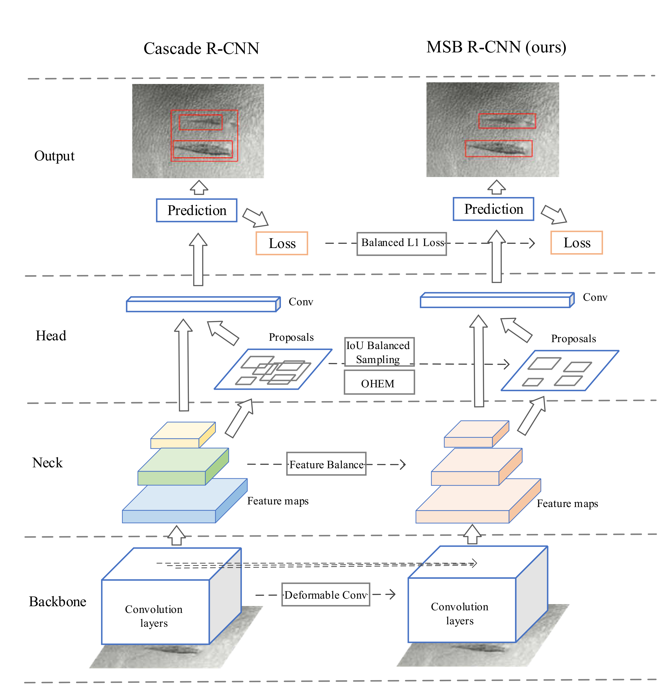
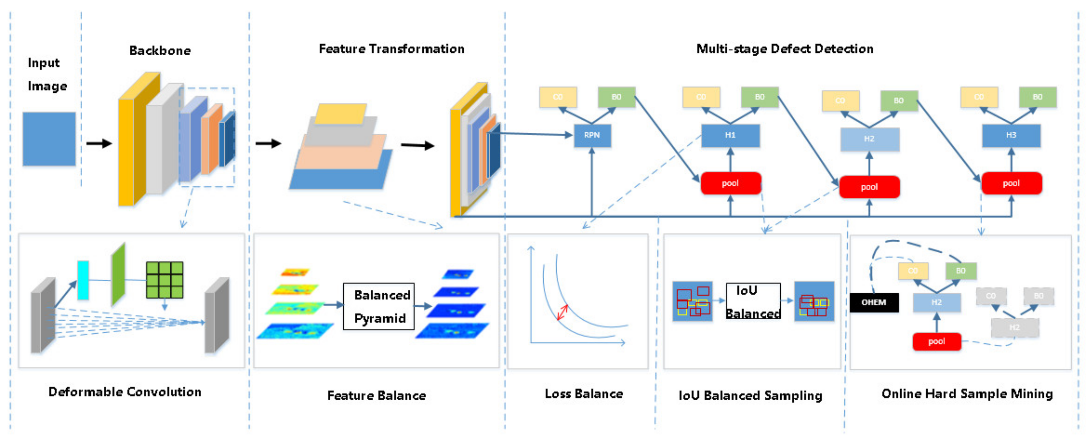
MSB R-CNN is an object detection network designed for defect detection. It can better balance the learning of the network and effectively improve the detection accuracy. The network includes five parts, which can be seen in Figure 1: backbone network, feature transformation pyramid, multi-stage detection head, the loss functions, and sampling strategies of the training process. The following subsections will focus on the deformable convolution in the backbone network, the balanced feature pyramid, the staged balanced L1 loss, and the sample selection strategy.
3.1. Deformable Convolution for Defect Detection
Convolutional neural networks have an inherent deficiency in the modeling of large and unknown shape transformations. This deficiency comes from the geometric structure of the convolution module: the convolution unit samples the fixed position of the input feature map, and the pooling layer is performed at a fixed ratio. Even the area of interest pooling segments the area of interest into fixed areas. These characteristics are influential, as the shapes of the defect object in the defect detection may have great differences in shapes. Deformable convolution and deformable region of interest pooling can effectively improve the ability of the modeling defect deformation. Figure 2 shows that the appropriate addition of variable-shape convolution to the backbone convolutional network can improve the adaptability of the network for different shapes of defects. The integration of deformable convolution to the backbone network not only effectively improves the extraction of defect shape features, but also regulates the number of parameters.
3.2. Feature Balance Transformation
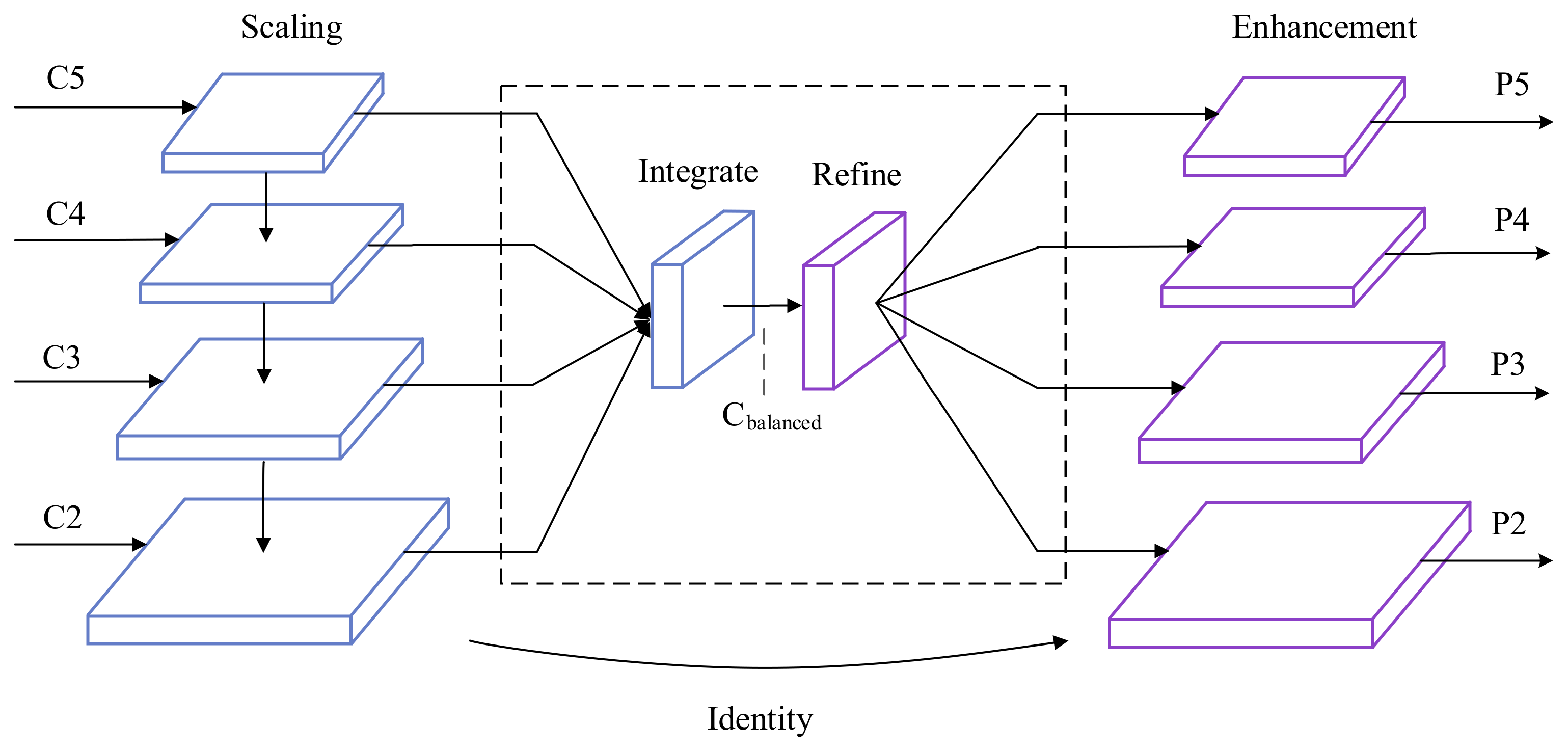
The high-level features extracted by the backbone network have more semantic meaning, while the low-level features have more descriptive content. Both level features have a huge impact on defect detection. Therefore, the method of integrating the high-level and low-level characteristics of defects in MSB R-CNN is particularly important. The feature integration through horizontal connections in FPN [13] and PANet [37] promotes the development of defect detection. However, the integrated feature maps are not balanced from each resolution. Different from using horizontal connections to integrate multi-level features, the key to feature balance is to use the same deep integration of each resolution to balance semantic features to enhance multi-level features [14]. It consists of four steps: scaling, integration, refinement and enhancement, as shown in Figure 3. The feature with a -level resolution is denoted as . In Figure 3, has the largest resolution. In order to integrate multi-level features and retain their semantic hierarchical structure, we first reshape the multi-level features to an intermediate size, i.e., the same size as , with interpolation and maximum pooling. Once the features are rescaled, the balanced semantic features are obtained by the following average formula:
where denotes the number of multi-level features, and and are denoted as the lowest and highest levels indicators involved. Then, we further refine the balanced semantic features by an embedded Gaussian non-local attention module [41], to make the features more discriminative. After refinement, the features are restored to the original feature map sizes through up-sampling or down-sampling. Then, each one passes through a 3 × 3 convolution for enhancement. Using this method, features from low-level to high-level are aggregated at the same time. The output is used for object detection in the same pipeline as in FPN. Therefore, by feeding these balanced features to the multi-stage detector, the performance of defect detection can be improved.
3.3. Staged Balanced Loss
A defect detector usually needs to perform the classification task and localization task; hence, there is a tradeoff to balance the classification loss and location loss during training process. If the two losses are not balanced, the training effect will be affected. There are also imbalances between simple samples and hard samples. The difficulty of the sample represents the difficulty of the sample to be detected, and usually the difficulty of small targets is greater than that of large targets. If they are not properly balanced, the small gradients produced by simple samples may be submerged by the large gradients produced by hard samples, which will limit the ability for further refinement. Therefore, the losses and samples both need to be rebalanced to achieve the best convergence.
Let us first review the commonly used smooth L1 loss. Smooth L1 loss is defined as follows:
where is the absolute difference between the predicted value and the true value of the target bounding box coordinate. However, the gradients of the outliers still have a negative effect on learning the inliers with smaller gradients in smooth L1 loss. To solve this problem, balanced L1 loss [14] considers the gradient balance across inliers and outliers, and clips the large gradients produced by outliers. After adding gradient restriction to the derivative equation of smooth L1 loss, the gradient formulation of balanced L1 loss can be defined as follows:
where represents the contribution of inliers, and is the upper bound of the error of outliers to balance the tasks. According to Equation (3), can be obtained as follows [14]:
where is used to ensure is continuous at , C is a constant, and the condition between the parameters is the following:
The effect of the loss function in different detection stages of MSB R-CNN is different. The experimental results seem to indicate that applying the balanced L1 loss to the first and second stages can achieve the best results.
3.4. Sample Screening Strategy
In the process of model training, a lot of regional suggestions are proposed, and the positive and negative samples are distinguished according to the IoU of the original marked bounding box. Assuming that the threshold is set to 0.5, the samples with the IoU in the interval of [0.5, 1] are marked as positive samples, and those with IoU in the interval of [0, 0.5) are marked as negative samples. Most of the regional suggestions are negative samples, which cause a large number of meaningless negative samples to cover a few meaningful positive samples, especially in the multi-stage process in MSB R-CNN. Therefore, the method of constructing the sampling mechanism has a great impact on the training and accuracy of the model.
If there are no objects identified in the regional proposals, all these proposals are considered as the background. Then, the classifier can easily and correctly classify them into the background. The following case is also called a simple sample, that is, the IoU of the regional proposal and the original marked box is between [0, 0.1]. In this case, the object has few features and is easy to be classified. If the IoU of the regional proposal and the original marker box is close to but less than 0.5, such as 0.4, the regional proposal is considered a negative sample. However, this sample is closer to the original marked box. In this case, this sample becomes a hard sample. Another intuitive indicator to distinguish simple samples from hard samples is the loss value of the sample. The larger the loss value is, the more difficult the sample is to be detected correctly.
In view of this, OHEM and Focal loss are the main methods to solve the sample imbalance problem. OHEM automatically selects hard samples according to their confidence. This process significantly increases the use of memory and computational costs. In addition, there are still noisy samples in OHEM and during the sampling process, so it does not work well in some cases. Focal loss uses an elegant loss function to solve the problem of the imbalance of additional foreground categories in the single-stage detector. However, this brings little improvement on multi-stage detectors, due to the differences between multiple types of imbalances.
In order to overcome the disadvantages of OHEM and Focal loss, the IoU balanced sampling [35] takes into account the relationship between IoU and sample difficulty. The public statistical data [14] show that more than 60% of the hard samples have IoU values that are greater than 0.05, compared to the original marked box. However, only 30% of the samples selected by the random sampler have IoU values greater than 0.05. This also indicates that random sampler can easily lead to unbalanced samples with many hard samples being buried in a large number of simple samples. Based on this observation, the IoU balance sampling strategy is applied for mining hard samples.
4. Experimental Results and Analysis
Data sets: This paper conducts training and testing on the DAGM2007 data set [10] and GC10 data set [42].
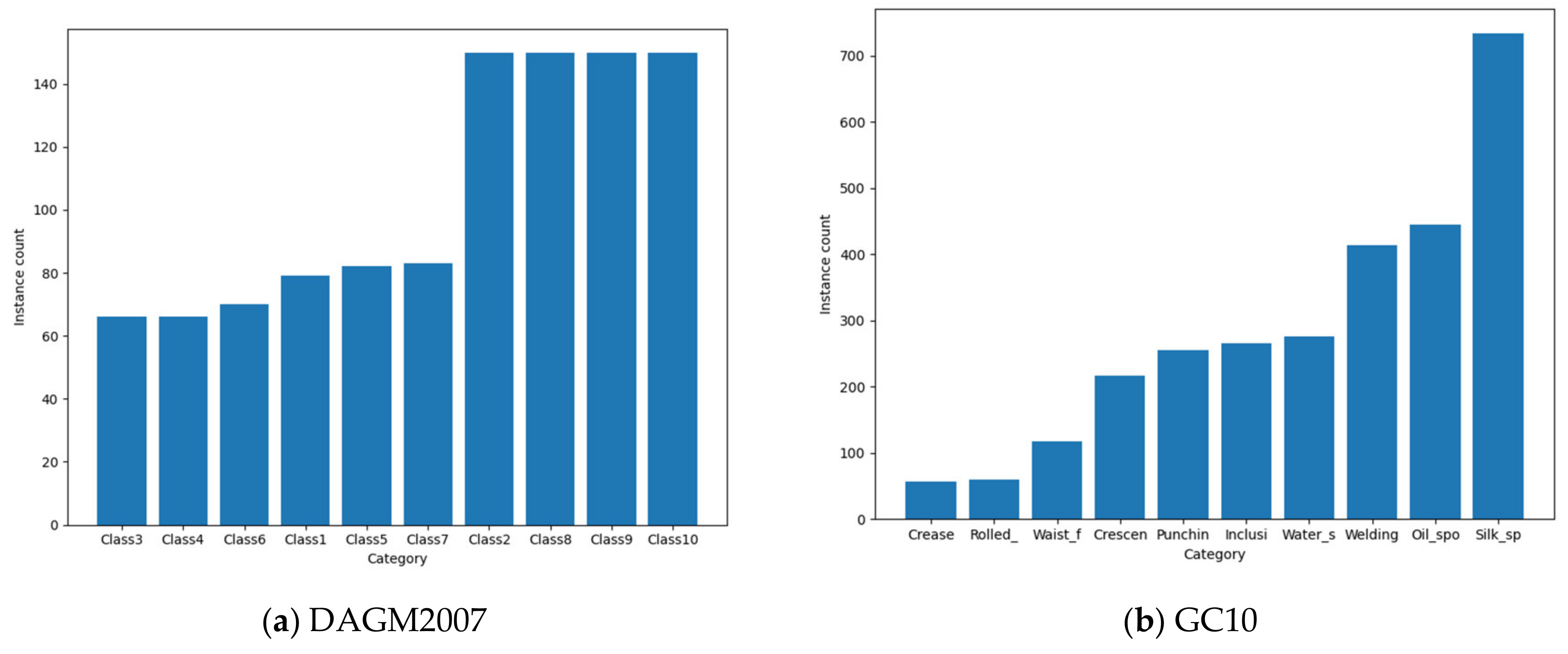
- The DAGM2007 data set is used to detect miscellaneous defects on various background textures. It contains 10 categories of different kinds of defects. Both training set and test set consist of 1000 images with one labeled defect each on the background texture. The class distribution of samples in DAGM2007 training set is shown in Figure 4a.
- The GC10 data set contains 10 categories of different types of steel surface defects, for steel defect detection. It consists of 2000 images in the training set and 500 images in the test set. Each image has multiple labeled defects. The class distribution of samples in the GC10 training set is shown in Figure 4b.
Training settings: The optimizer used in training is Stochastic Gradient Descent (SGD); the basic learning rate is 0.02; the momentum factor is 0.9; and the weight decay factor is set to 0.0001. In the initial 500 iterations, a linear warm-up is used to increase the learning rate from 0.0001 to the basic learning rate. A total of 40 epochs are trained, and a multi-stage learning rate decay strategy is adopted, which reduces the learning rate to 10% at 16 and 38 epochs, respectively. Then, we save the model, test the results in each period, and calculate its mAP and the AP of each AR of targets. The stop condition is either the loss stops decreasing or the validation accuracy reaching the peak, whichever condition comes first. The above settings are directly taken from mmdetection [43]. All models use the same training settings in both databases.
4.1. Experiments on DAGM2007
Table 1 shows the overall defect detection performances of MSB R-CNN compared with the experimental results of the previous mainstream single-stage detection algorithms SSD, RetainNet, and multi-stage detection algorithms, Faster R-CNN, Grid R-CNN, Cascade R-CNN and Libra R-CNN. Our network obtains the highest accuracy of 67.5%, which is 1.5% higher than that of Cascade R-CNN. On the AP50 value, although we do not achieve the best results, the detection accuracy reaches 98.9%, which is above the expectation of the industrial application (usually above 95% is acceptable for industrial applications). The mAP of MSB R-CNN on the AP75 project achieves the best accuracy of 79.8%. In the defect detection of medium and large defects, the mAP of our network reaches the best accuracy of 65.8% and 69%, indicating that MSB R-CNN has a better detection effect for medium and large objects but less so for detecting small objects.
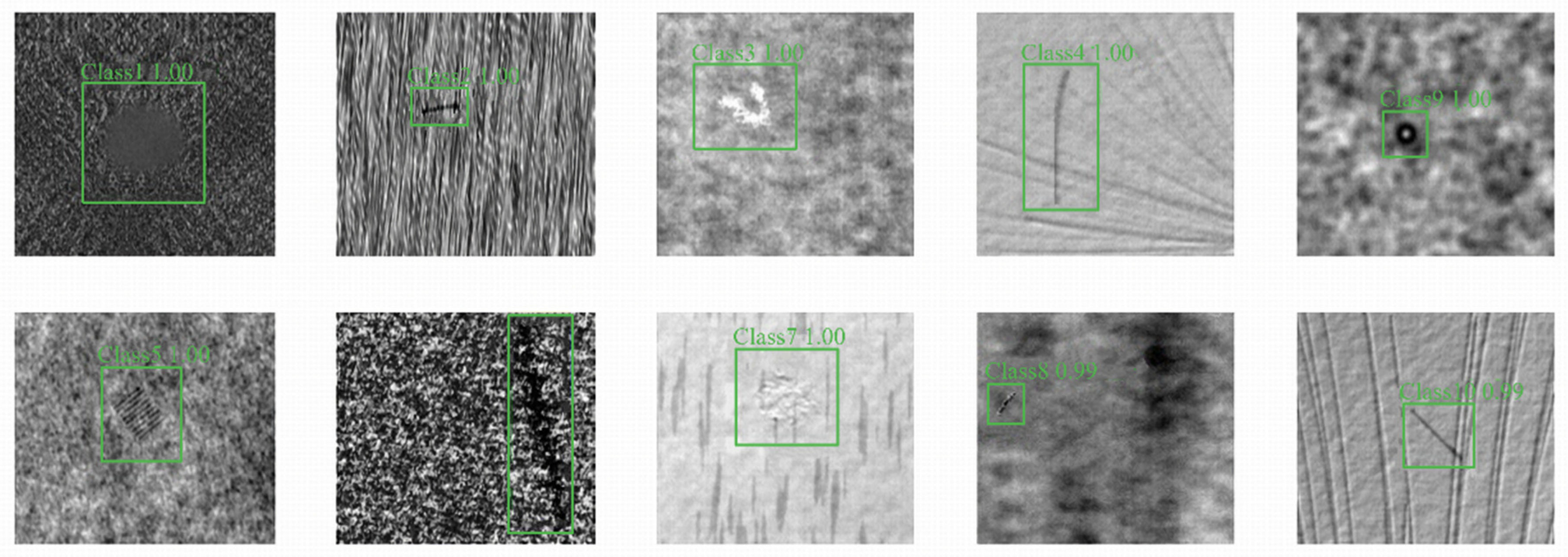
Next, we analyze the detection effect of each category. Table 2 compares the results of each class of defect detection with the state of the art one-stage detection algorithms, i.e., SSD, RetainNet and multi-stage detection algorithms, Faster R-CNN, Grid R-CNN, Cascade R-CNN and Libra R-CNN. In the accuracy of the second, fifth, seventh, and tenth classes, MSB R-CNN achieves the best result. Especially in the tenth category, the mAP of 76.7% achieved by our network significantly outperforms other algorithms. It can also be seen from Figure 5 that these are larger targets. The third type of object is relatively small, and the edges are more complex. The results achieved by our algorithm are much better than those of others.
4.2. Experiments on GC10
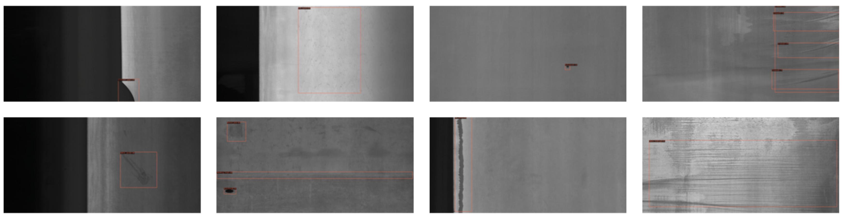
In order to verify the performance of the model in data sets of varying complexity, we also evaluate our model and other state-of-the-art models on the GC10 data set, which has much greater complexity than DAGM2007. Since the number of samples with a small area is few in GC10 data set, we ignore the APS. As shown in Table 3, our model MSB R-CNN obtains the highest mAP of 34.0%, compared to Faster R-CNN, Grid R-CNN, RetinaNet, Cascade R-CNN, SSD and Libra R-CNN. Compared with Cascade R-CNN, the mAP of MSB R-CNN is 0.6% higher. MSB R-CNN achieves the best accuracy both in AP50 and AP75. However, there is no advantage for MSB R-CNN on APM. Table 4 shows the comparison of accuracy in each category. MSB R-CNN achieves the best results in the second, fourth, fifth, sixth, eighth, and tenth categories. The visualization of the MSB R-CNN prediction results is shown in Figure 6.
4.3. Ablation Study
All ablation experiments are based on the DAGM2007 data set. We train the models on the training subset and test on the test subset.
4.3.1. Effectiveness of Our Method
We perform ablation experiments to prove the influence of each module on the accuracy of MSB R-CNN. Table 5 summarizes the experimental results of multiple sets of ablation experiments, where the baseline is Cascade R-CNN, dcn represents a deformable convolutional network, bf represents feature balance, bl represents balanced loss, and sam represents a combination of OHEM and IoU balanced sampling. The baseline’s mAP is 66.0% After adding deformable convolution, the mAP of our network is increased to 66.5%, and the mAP for detection of small defects reaches the highest of 62.6%. With the deformable convolution, the feature balance is performed, and the mAP of the network reaches 66.7%. After the feature is balanced, the loss is also balanced at a specific stage, and the mAP of the network reaches 67.0%. Finally, on the basis of the previous network, the sampling is selected in stages for IoU balanced sampling and OHEM sampling, making the network’s mAP reaches a maximum of 67.5%, which is 1.5% higher than the benchmark. Moreover, the ability to detect large-scale defects reaches the highest level.
4.3.2. Impact of Fusion Deformable Convolution Parameters
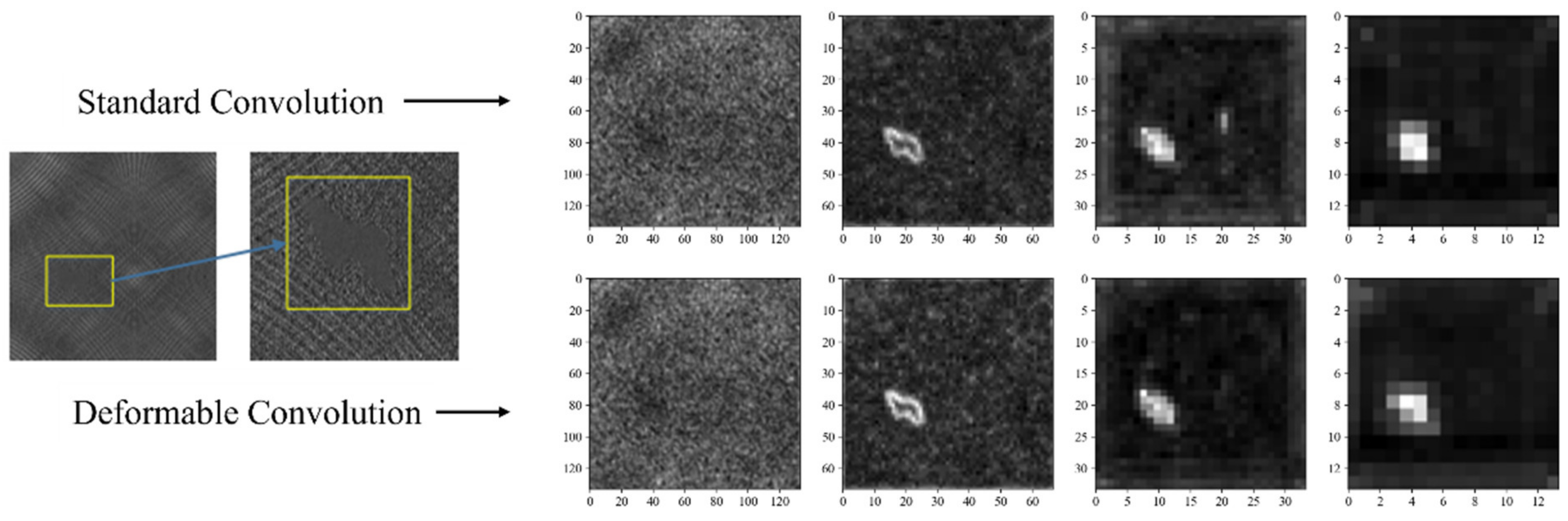
It can be seen from Table 6 that adding deformable convolution in the first and third stages can obtain the highest mAP of 66.6%; the number of parameters is also increased by 0.33 M, compared to the benchmark. The more deformable convolutions are added, the larger the number of the parameters. The feature map comparison between deformable convolution and standard convolution is given in Figure 7.
4.3.3. Impact of Feature Balance Transformation
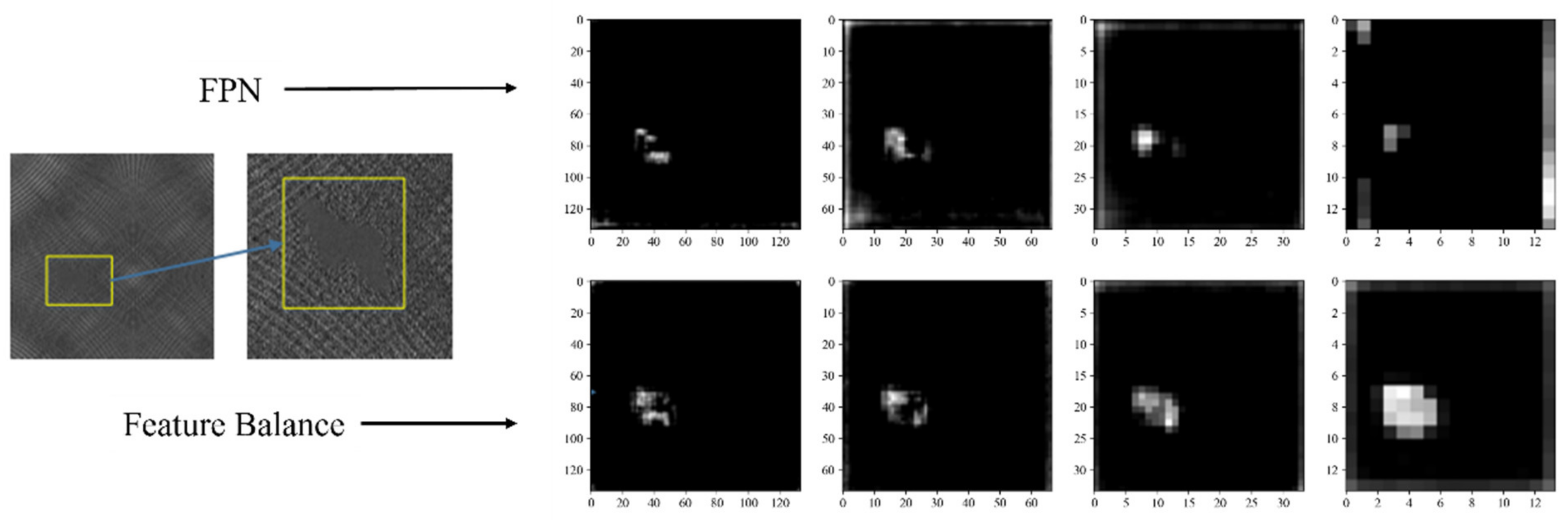
As seen from Table 7, although the value of mAP does not increase much after feature balancing, the APS is increased from 60.7% to 63.0%. This shows that feature imbalance mainly occurs in small targets. At the same time, the detection accuracy of each size is improved to different degrees. Figure 8 shows that the balanced feature has a higher degree of recognition.
4.3.4. Impact of Staged Loss Balance Parameters
Balanced L1 loss balances the contribution of difficult and simple samples to make the network converge better. It can be seen from Table 8 that applying balanced L1 loss in all three stages does not promise better results, as mAP drops to 65.9%. When the balanced L1 loss is applied in the first and second stages, the detection accuracy is the highest where the mAP reaches 66.7%. Therefore, we apply balanced L1 loss in the first and second stages of MSB R-CNN to achieve better results.
4.3.5. Impact of Construction Sample Screening Method
First, we analyze the impact of OHEM sampling on defect detection. The experimental results are shown in Table 9. Applying OHEM at every stage is not the most effective. That is because OHEM is used to sort the recommended regions with larger losses, and then choose to learn the recommended regions with larger losses. The influence of noise on the recommended regions is still unavoidable. Therefore, adding OHEM in specific stages can improve detection performance, but adding it in all stages will result in a decrease in detection accuracy. Moreover, Table 9 also shows that setting OHEM in one stage is usually better than setting OHEM in multiple stages. So, we apply OHEM in the first stage of MSB R-CNN.
Next, we analyze the impact of IoU balanced sampling on defect detection. Table 10 shows that IoU balanced sampling can effectively improve the accuracy of the network. The mAP of IoU balanced sampling in the first and third stages and IoU balanced sampling in the first and second stages is 66.6%. Using IoU balanced sampling for all three stages, the mAP is 66.5%. On considering the accuracy and complexity, we apply IoU balanced sampling in the first and second stages.
Here, we analyze the influence of OHEM sampling and IoU balanced sampling on defect detection. From the experimental results in Table 11, it can be concluded that the usage of three different sampling methods has a greater impact on the accuracy of the network. From the results, the optimal setting is to apply the IoU balanced sampling in the first and second stages and use OHEM in the third stage. In this case, we can obtain the best results, and the mAP reaches 66.8%.
5. Conclusions
In the face of complex defect types, it is difficult for general object detection networks to achieve accurate detection. We optimized Cascade R-CNN for defect detection task and proposed MSB R-CNN, which can better balance the learning of the network and effectively improve the detection accuracy. MSB R-CNN adopts deformable convolution in backbone network to improve the detection accuracy of defects with different shapes and uses balanced feature pyramid to make high-level and low-level features more balanced. During training, the balanced L1 loss is applied to better balance the learning benefits between different tasks, and IoU balanced sampling is used to balance the hard samples and simple samples. Based on the network architecture design and experiment results, MSB R-CNN shows more advantages in terms of accuracy and network balance than other popular detection networks. MSB R-CNN uses a multi-stage detector, which is suitable for high-precision detection, but it is relatively time-consuming. In the future, the proposed method can be further applied to a single-stage detector to meet the needs of real-time detection.
Author Contributions
Z.X., S.L. and Z.Y. implemented the proposed method, analyzed results and drafted the paper; Z.X., S.L. and J.C. conceived and designed the experiments; J.C. analyzed results and also revised the paper with Z.W. and Y.C. All authors have read and agreed to the published version of the manuscript.
Funding
This work is supported in part by the Grants of National Key R&D Program of China 2020AAA0108304, the Science and Technology Project of Guangdong Province (No. 2019A050513011), Guangzhou Science and Technology Plan Project (No. 202002030386), National Natural Science Foundation of China (U1911401, U1701261), and Guangdong Provincial Key Laboratory of Intellectual Property and Big Data under Grant (No. 2018B030322016).
Conflicts of Interest
The authors declare no conflict of interest.
References
- Ngan, H.Y.T.; Pang, G.K.H.; Yung, N.H.C. Automated fabric defect detection—A review. Image Vis. Comput. 2011, 29, 442–458. [Google Scholar] [CrossRef]
- Yang, J.; Li, S.; Wang, Z. Real-time tiny part defect detection system in manufacturing using deep learning. IEEE Access 2019, 7, 89278–89291. [Google Scholar] [CrossRef]
- Xiao, Z.; Nguyen, M.; Maggard, E. Real-time print quality diagnostics. Electron. Imaging 2017, 2017, 174–179. [Google Scholar] [CrossRef]
- Kim, S.; Jo, Y.; Cho, J. Spatially Variant Convolutional Autoencoder Based on Patch Division for Pill Defect Detection. IEEE Access 2020, 8, 216781–216792. [Google Scholar] [CrossRef]
- Wei, X.; Yang, Z.; Liu, Y. Railway track fastener defect detection based on image processing and deep learning techniques: A comparative study. Eng. Appl. Artif. Intell. 2019, 80, 66–81. [Google Scholar] [CrossRef]
- Valero, E.; Forster, A.; Bosché, F. Automated defect detection and classification in ashlar masonry walls using machine learning. Autom. Constr. 2019, 106, 102846. [Google Scholar] [CrossRef]
- Cai, Z.; Vasconcelos, N. Cascade r-cnn: Delving into high quality object detection. In Proceedings of the IEEE Conference on Computer Vision and Pattern Recognition, Salt Lake City, UT, USA, 18–22 June 2018; pp. 6154–6162. [Google Scholar]
- Zhao, Z.Q.; Zheng, P.; Xu, S. Object detection with deep learning: A review. IEEE Trans. Neural Netw. Learn. Syst. 2019, 30, 3212–3232. [Google Scholar] [CrossRef] [PubMed] [Green Version]
- Lu, X.; Li, B.; Yue, Y. Grid R-CNN. In Proceedings of the IEEE/CVF Conference on Computer Vision and Pattern Recognition, Long Beach, CA, USA, 15–20 June 2019; pp. 7363–7372. [Google Scholar]
- Wieler, M.; Hahn, T. Weakly supervised learning for industrial optical inspection. In Proceedings of the 29th Annual Symposium of the German Association for Pattern Recognition (DAGM 2007), Heidelberg, Germany, 12–14 September, 2007. [Google Scholar]
- Oksuz, K.; Cam, B.C.; Kalkan, S.; Akbas, E. Imbalance Problems in Object Detection: A Review. IEEE Trans. Pattern Anal. Mach. Intell. 2020. [Google Scholar] [CrossRef] [PubMed] [Green Version]
- Dai, J.; Qi, H.; Xiong, Y. Deformable convolutional networks. In Proceedings of the IEEE International Conference on Computer Vision, Venice, Italy, 22–29 October 2017; pp. 764–773. [Google Scholar]
- Lin, T.Y.; Dollár, P.; Girshick, R. Feature pyramid networks for object detection. In Proceedings of the IEEE Conference on Computer Vision and Pattern Recognition, Honolulu, HI, USA, 21–26 July 2017; pp. 2117–2125. [Google Scholar]
- Pang, J.; Chen, K.; Shi, J. Libra r-cnn: Towards balanced learning for object detection. In Proceedings of the IEEE/CVF Conference on Computer Vision and Pattern Recognition, Long Beach, CA, USA, 15–20 June 2019; pp. 821–830. [Google Scholar]
- Girshick, R. Fast r-cnn. In Proceedings of the IEEE International Conference on Computer Vision, Santiago, Chile, 7–13 December 2015; pp. 1440–1448. [Google Scholar]
- Lin, T.Y.; Goyal, P.; Girshick, R. Focal loss for dense object detection. In Proceedings of the IEEE International Conference on Computer Vision, Venice, Italy, 22–29 October 2017; pp. 2980–2988. [Google Scholar]
- Shrivastava, A.; Gupta, A.; Girshick, R. Training region-based object detectors with online hard example mining. In Proceedings of the IEEE Conference on Computer Vision and Pattern Recognition, Las Vegas, CA, USA, 26 June–1 July 2016; pp. 761–769. [Google Scholar]
- Girshick, R.; Donahue, J.; Darrell, T. Rich feature hierarchies for accurate object detection and semantic segmentation. In Proceedings of the IEEE Conference on Computer Vision and Pattern Recognition, Columbus, OH, USA, 23–28 June 2014; pp. 580–587. [Google Scholar]
- Van Everingham, M.; Gool, L.; Williams, C.K.I. The pascal visual object classes (voc) challenge. Int. J. Comput. Vis. 2010, 88, 303–338. [Google Scholar] [CrossRef] [Green Version]
- He, K.; Zhang, X.; Ren, S. Spatial pyramid pooling in deep convolutional networks for visual recognition. IEEE Trans. Pattern Anal. Mach. Intell. 2015, 37, 1904–1916. [Google Scholar] [CrossRef] [PubMed] [Green Version]
- Zeiler, M.D.; Fergus, R. Visualizing and understanding convolutional networks. In European Conference on Computer Vision; Springer: Cham, Switzerland, 2014; pp. 818–833. [Google Scholar]
- Ren, S.; He, K.; Girshick, R. Faster R-CNN: Towards real-time object detection with region proposal networks. Adv. Neural Inf. Process. Syst. 2015, 28, 91–99. [Google Scholar] [CrossRef] [PubMed] [Green Version]
- Chen, K.; Pang, J.; Wang, J. Hybrid task cascade for instance segmentation. In Proceedings of the IEEE/CVF Conference on Computer Vision and Pattern Recognition, Long Beach, CA, USA, 15–20 June 2019; pp. 4974–4983. [Google Scholar]
- He, K.; Gkioxari, G.; Dollár, P. Mask r-cnn. In Proceedings of the IEEE International Conference on Computer Vision, Venice, Italy, 22–29 October 2017; pp. 2961–2969. [Google Scholar]
- Liu, W.; Anguelov, D.; Erhan, D. SSD: Single shot multibox detector. In European Conference on Computer Vision; Springer: Cham, Switzerland, 2016; pp. 21–37. [Google Scholar]
- Redmon, J.; Farhadi, A. Yolov3: An incremental improvement. arXiv 2018, arXiv:1804.02767. [Google Scholar]
- Bochkovskiy, A.; Wang, C.Y.; Liao, H.Y.M. Yolov4: Optimal speed and accuracy of object detection. arXiv 2020, arXiv:2004.10934. [Google Scholar]
- Ouyang, W.; Wang, K.; Zhu, X. Chained cascade network for object detection. In Proceedings of the IEEE International Conference on Computer Vision, Venice, Italy, 22–29 October 2017; pp. 1938–1946. [Google Scholar]
- Hu, H.; Gu, J.; Zhang, Z. Relation networks for object detection. In Proceedings of the IEEE Conference on Computer Vision and Pattern Recognition, Salt Lake City, UT, USA, 18–22 June 2018; pp. 3588–3597. [Google Scholar]
- Singh, B.; Davis, L.S. An analysis of scale invariance in object detection snip. In Proceedings of the IEEE Conference on Computer Vision and Pattern Recognition, Salt Lake City, UT, USA, 18–22 June 2018; pp. 3578–3587. [Google Scholar]
- Zhu, X.; Pang, J.; Yang, C. Adapting object detectors via selective cross-domain alignment. In Proceedings of the IEEE/CVF Conference on Computer Vision and Pattern Recognition, Long Beach, CA, USA, 15–20 June 2019; pp. 687–696. [Google Scholar]
- Zeng, X.; Ouyang, W.; Yan, J. Crafting gbd-net for object detection. IEEE Trans. Pattern Anal. Mach. Intell. 2017, 40, 2109–2123. [Google Scholar] [CrossRef] [PubMed] [Green Version]
- Zhu, X.; Hu, H.; Lin, S. Deformable convnets v2: More deformable, better results. In Proceedings of the IEEE/CVF Conference on Computer Vision and Pattern Recognition, Long Beach, CA, USA, 15–20 June 2019; pp. 9308–9316. [Google Scholar]
- Cao, Y.; Chen, K.; Loy, C.C. Prime sample attention in object detection. In Proceedings of the IEEE/CVF Conference on Computer Vision and Pattern Recognition, Seattle, WA, USA, 14–19 June 2020; pp. 11583–11591. [Google Scholar]
- Yu, F.; Koltun, V. Multi-scale context aggregation by dilated convolutions. arXiv 2015, arXiv:1511.07122. [Google Scholar]
- Li, Y.; Chen, Y.; Wang, N. Scale-aware trident networks for object detection. In Proceedings of the IEEE/CVF International Conference on Computer Vision, Seoul, Korea, 27–28 October 2019; pp. 6054–6063. [Google Scholar]
- Liu, S.; Qi, L.; Qin, H. Path aggregation network for instance segmentation. In Proceedings of the IEEE Conference on Computer Vision and Pattern Recognition, Salt Lake City, UT, USA, 18–22 June 2018; pp. 8759–8768. [Google Scholar]
- He, Y.; Zhu, C.; Wang, J. Bounding box regression with uncertainty for accurate object detection. In Proceedings of the IEEE/CVF Conference on Computer Vision and Pattern Recognition, Long Beach, CA, USA, 15–20 June 2019; pp. 2888–2897. [Google Scholar]
- Cao, J.; Pang, Y.; Han, J. Hierarchical shot detector. In Proceedings of the IEEE/CVF International Conference on Computer Vision, Seoul, Korea, 27–28 October 2019; pp. 9705–9714. [Google Scholar]
- Rezatofighi, H.; Tsoi, N.; Gwak, J.Y. Generalized intersection over union: A metric and a loss for bounding box regression. In Proceedings of the IEEE/CVF Conference on Computer Vision and Pattern Recognition, Long Beach, CA, USA, 15–20 June 2019; pp. 658–666. [Google Scholar]
- Wang, X.; Girshick, R.; Gupta, A. Non-local neural networks. In Proceedings of the IEEE Conference on Computer Vision and Pattern Recognition, Salt Lake City, UT, USA, 18–22 June 2018; pp. 7794–7803. [Google Scholar]
- GC10. Available online: https://aistudio.baidu.com/aistudio/datasetdetail/89446/0 (accessed on 21 May 2021).
- Chen, K.; Wang, J.; Pang, J. MMDetection: Open mmlab detection toolbox and benchmark. arXiv 2019, arXiv:1906.07155. [Google Scholar]
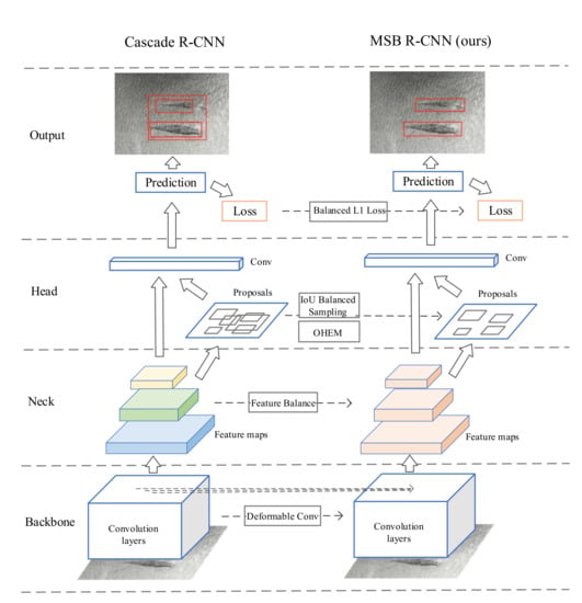
Figure 1.
Multi-stage balanced R-CNN (MSB R-CNN) network framework. The backbone of the network incorporates deformable convolution to balance high-level and low-level features. The balanced features then pass through the three-stage detector. The loss balancing is carried out in each stage where different sampling methods are adopted at different stages.

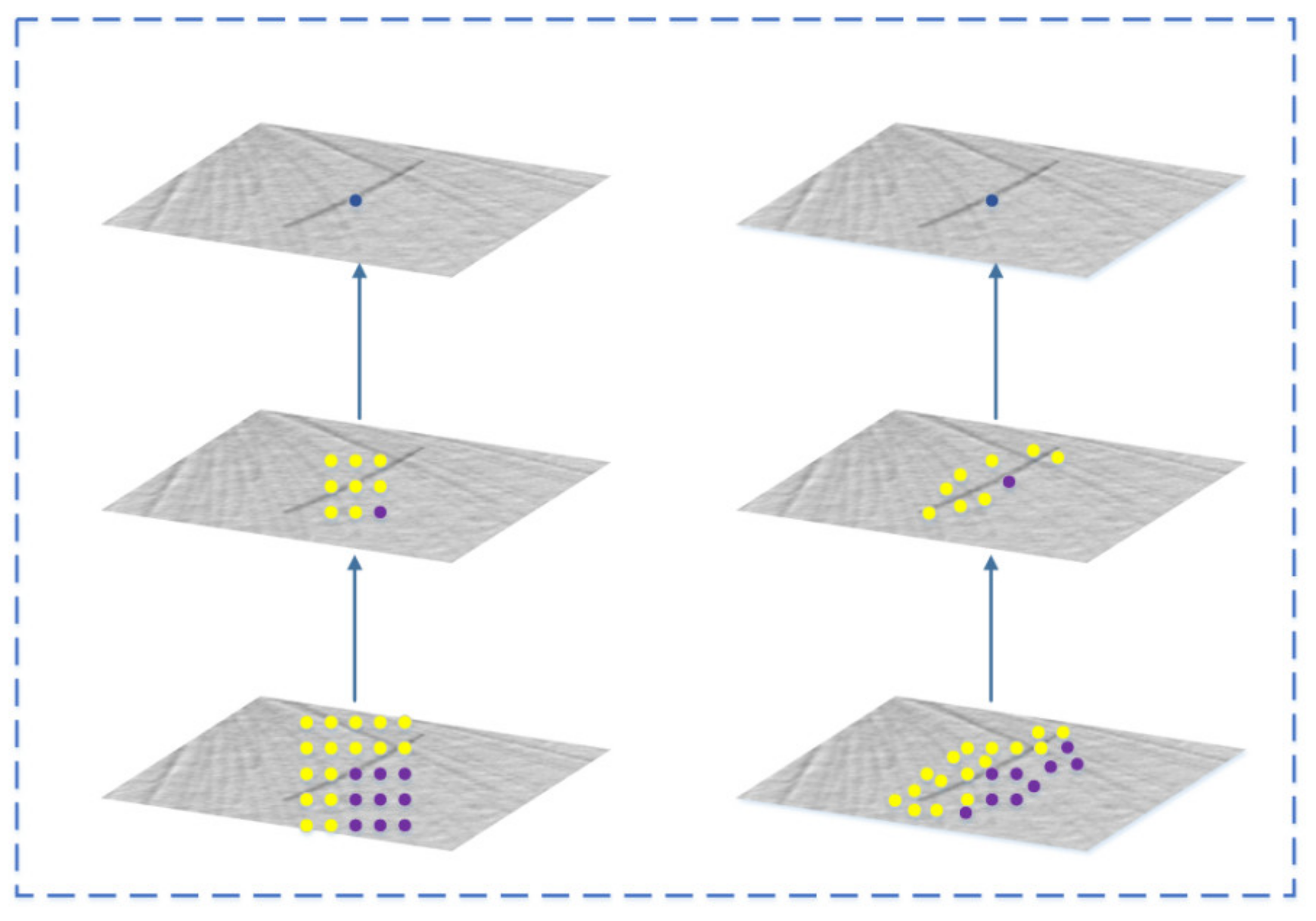
Figure 2.
Regular convolution (left) and deformable convolution (right) for defect images. Unlike regular convolution, which uses a fixed-shape convolution kernel, deformable convolution calculates offsets and the orientation for sampling points, which makes the shape of the convolution kernel variable, thereby improving the ability to extract shape features.

Figure 3.
Pipeline and heat map visualization of balanced feature pyramid. C1–C5 represent different levels of feature maps output from the backbone network and C2–C5 are used for feature integration. With multi-scale feature integration and refinement, we obtain the balanced feature pyramid. Finally, identity connect is performed, that is, adding the original features to the output.

Figure 4.
The class distribution of samples in the training set of (a) DAGM2007 and (b) GC10.

Figure 5.
Examples of detection result on DAGM2007 data set.

Figure 6.
Examples of detection result on GC10 data set.

Figure 7.
Feature comparison of deformable convolution and standard convolution. Judging from the features of the four stages extracted from the backbone network, the deformable convolution fits the shape of the defect better than the original convolution in the last stage.
Figure 7.
Feature comparison of deformable convolution and standard convolution. Judging from the features of the four stages extracted from the backbone network, the deformable convolution fits the shape of the defect better than the original convolution in the last stage.

Figure 8.
Comparison of balanced feature and FPN feature. The features after feature balance is strengthened, and the defect area is more obvious.
Figure 8.
Comparison of balanced feature and FPN feature. The features after feature balance is strengthened, and the defect area is more obvious.


Table 1.
Detection accuracy in DAGM2007 (%). mAP is AP (IoU = 0.5:0.95, AR = all), AP50 is AP (IoU = 0.5, AR = all), AP75 is AP (IoU = 0.75, AR = all), APS is AP (IoU = 0.5:0.95, AR = S), APM is AP (IoU = 0.5:0.95, AR = M), and APL is AP (IoU = 0.5:0.95, AR = L). AR is the average recall for objects, AR = S is AR for small objects (area < ), AR = M is AR for medium objects ( < area < ), and AR = L is AR for large objects (area > ).
| AP | Faster R-CNN [22] | Grid R-CNN [9] | RetinaNet [28] | Cascade R-CNN [7] | SSD [25] | Libra R-CNN [14] | Ours |
|---|---|---|---|---|---|---|---|
| mAP | 64.6 | 66.5 | 65.2 | 66.0 | 63.2 | 66.7 | 67.5 |
| AP50 | 99.1 | 98.7 | 99.4 | 99.2 | 98.6 | 98.9 | 98.9 |
| AP75 | 74.5 | 78.9 | 75.5 | 77.6 | 73.3 | 77.7 | 79.8 |
| APS | 54.7 | 56.7 | 57.1 | 60.7 | 55.9 | 61.6 | 60.1 |
| APM | 63.2 | 65.8 | 63.5 | 64.7 | 62.8 | 65.6 | 65.8 |
| APL | 66.0 | 67.4 | 65.2 | 66.8 | 65.5 | 66.1 | 69.0 |
Table 2.
Detection accuracy (%) in each category (mAP).
| Class | Faster R-CNN [22] | Grid R-CNN [9] | RetinaNet [28] | Cascade R-CNN [7] | SSD [25] | Libra R-CNN [14] | Ours |
|---|---|---|---|---|---|---|---|
| Class1 | 60.5 | 63.2 | 62.5 | 63.1 | 52.6 | 63.5 | 62.4 |
| Class2 | 64.4 | 68.3 | 66.9 | 66.2 | 67.3 | 70.1 | 70.8 |
| Class3 | 56.5 | 55.0 | 56.0 | 56.4 | 56.1 | 57.0 | 54.3 |
| Class4 | 69.2 | 72.2 | 70.2 | 66.5 | 68.5 | 68.3 | 70.9 |
| Class5 | 69.6 | 73.6 | 72.8 | 72.0 | 71.7 | 71.5 | 74.2 |
| Class6 | 70.6 | 70.7 | 71.7 | 75.4 | 65.8 | 73.9 | 75.1 |
| Class7 | 58.8 | 63.4 | 60.9 | 62.8 | 59.5 | 62.8 | 65.1 |
| Class8 | 51.9 | 54.9 | 53.7 | 53.0 | 48.2 | 54.9 | 53.9 |
| Class9 | 72.2 | 70.7 | 69.8 | 69.8 | 69.7 | 71.0 | 71.2 |
| Class10 | 72.0 | 74.1 | 71.9 | 73.4 | 72.6 | 74.7 | 76.7 |
Table 3.
Detection accuracy in GC10 (%).
| AP | Faster R-CNN [22] | Grid R-CNN [9] | RetinaNet [28] | Cascade R-CNN [7] | SSD [25] | Libra R-CNN [14] | Ours |
|---|---|---|---|---|---|---|---|
| mAP | 29.7 | 27.9 | 25.6 | 33.4 | 24.7 | 29.1 | 34.0 |
| AP50 | 64.5 | 61.4 | 53.9 | 66.6 | 55.9 | 62.3 | 67.2 |
| AP75 | 25.8 | 20.3 | 21.3 | 30.7 | 19.7 | 23.1 | 32.7 |
| APS | - | - | - | - | - | - | - |
| APM | 18.2 | 18.2 | 16.7 | 18.3 | 14.7 | 17.5 | 17.5 |
| APL | 29.3 | 27.1 | 24.2 | 32.5 | 23.0 | 28.4 | 34.0 |
Table 4.
Detection accuracy (%) in each category (mAP).
| Class | Faster R-CNN [22] | Grid R-CNN [9] | RetinaNet [28] | Cascade R-CNN [7] | SSD [25] | Libra R-CNN [14] | Ours |
|---|---|---|---|---|---|---|---|
| Crease | 7.0 | 9.1 | 3.0 | 13.3 | 5.0 | 4.2 | 9.6 |
| Crescent_gap | 59.4 | 54.9 | 54.5 | 61.3 | 47.7 | 60.3 | 62.2 |
| Inclusion | 10.0 | 8.6 | 7.1 | 9.7 | 4.4 | 9.9 | 9.4 |
| Oil_spot | 25.4 | 22.2 | 22.9 | 24.2 | 16.5 | 22.6 | 26.6 |
| Punching | 54.0 | 54.3 | 53.5 | 54.2 | 52.0 | 54.5 | 54.8 |
| Rolled_pit | 16.0 | 16.5 | 2.6 | 15.9 | 6.0 | 17.7 | 19.6 |
| Silk_spot | 23.1 | 21.7 | 22.4 | 25.0 | 15.6 | 21.8 | 22.9 |
| Waist_folding | 34.6 | 35.5 | 30.6 | 36.2 | 22.0 | 30.8 | 41.8 |
| Water_spot | 41.2 | 40.5 | 40.1 | 44.0 | 33.5 | 41.5 | 42.9 |
| Welding_line | 26.6 | 16.0 | 22.2 | 49.9 | 44.7 | 27.9 | 50.4 |
Table 5.
Results of ablation experiments (%).
| AP | Baseline | Baseline + dcn | Baseline + dcn + bf | Baseline + dcn + bf + bl | Baseline + dcn + bf + bl + sam |
|---|---|---|---|---|---|
| mAP | 66.0 | 66.5 | 66.7 | 67.0 | 67.5 |
| AP50 | 99.2 | 99.1 | 98.7 | 98.6 | 98.9 |
| AP75 | 77.6 | 77.8 | 79.0 | 78.6 | 79.8 |
| APS | 60.7 | 62.6 | 59.1 | 59.7 | 60.1 |
| APM | 64.7 | 65.4 | 64.9 | 66.0 | 65.8 |
| APL | 66.8 | 66.4 | 68.3 | 65.5 | 69.0 |
Table 6.
Impact of deformable convolution being added at different stages (check symbol √ means deformable convolution being applied).
Table 6.
Impact of deformable convolution being added at different stages (check symbol √ means deformable convolution being applied).
| Experiment | Stage 1 | Stage 2 | Stage 3 | mAP@IoU = 0.5:0.95 (%) | Params(M) |
|---|---|---|---|---|---|
| 1 | 66.0 | 68.96 | |||
| 2 | √ | 66.5 | 69.04 | ||
| 3 | √ | 66.4 | 69.04 | ||
| 4 | √ | 66.5 | 69.04 | ||
| 5 | √ | √ | 66.3 | 69.29 | |
| 6 | √ | √ | 66.6 | 69.29 | |
| 7 | √ | √ | 66.1 | 69.29 | |
| 8 | √ | √ | √ | 66.5 | 69.54 |
Table 7.
Feature balance result (bf means feature balance).
| AP | Baseline | Baseline + bf |
|---|---|---|
| mAP | 66.0 | 66.3 |
| AP50 | 99.2 | 99.0 |
| AP75 | 77.6 | 77.9 |
| APS | 60.7 | 63.0 |
| APM | 64.7 | 65.1 |
| APL | 66.8 | 67.8 |
Table 8.
Experimental results of adding balanced L1 loss function at different stages (check symbol √ means applying balanced L1 loss function).
Table 8.
Experimental results of adding balanced L1 loss function at different stages (check symbol √ means applying balanced L1 loss function).
| Experiment | Stage 1 | Stage 2 | Stage 3 | mAP@IoU = 0.5:0.95 (%) |
|---|---|---|---|---|
| 1 | 66.0 | |||
| 2 | √ | 66.5 | ||
| 3 | √ | 66.5 | ||
| 4 | √ | 66.2 | ||
| 5 | √ | √ | 66.5 | |
| 6 | √ | √ | 66.6 | |
| 7 | √ | √ | 66.7 | |
| 8 | √ | √ | √ | 65.9 |
Table 9.
Experimental results of adding OHEM sampler in different stages (check symbol √ indicates OHEM is applied).
Table 9.
Experimental results of adding OHEM sampler in different stages (check symbol √ indicates OHEM is applied).
| Experiment | Stage 1 | Stage 2 | Stage 3 | mAP@IoU = 0.5:0.95 (%) |
|---|---|---|---|---|
| 1 | 66.0 | |||
| 2 | √ | 66.7 | ||
| 3 | √ | 66.5 | ||
| 4 | √ | 66.2 | ||
| 5 | √ | √ | 66.5 | |
| 6 | √ | √ | 66.7 | |
| 7 | √ | √ | 66.1 | |
| 8 | √ | √ | √ | 66.4 |
Table 10.
Experimental results of IoU balanced sampler in different stages (check symbol √ indicates IoU balanced sampling is applied).
Table 10.
Experimental results of IoU balanced sampler in different stages (check symbol √ indicates IoU balanced sampling is applied).
| Experiment | Stage 1 | Stage 2 | Stage 3 | mAP@IoU = 0.5:0.95 (%) |
|---|---|---|---|---|
| 1 | 66.0 | |||
| 2 | √ | 66.3 | ||
| 3 | √ | 66.0 | ||
| 4 | √ | 66.3 | ||
| 5 | √ | √ | 66.4 | |
| 6 | √ | √ | 66.6 | |
| 7 | √ | √ | 66.6 | |
| 8 | √ | √ | √ | 66.5 |
Table 11.
Experimental results of adding IoU balance and OHEM sampler combination in different stages (check symbol √ indicates IoU balanced sampling is applied; otherwise, OHEM sampler is used).
Table 11.
Experimental results of adding IoU balance and OHEM sampler combination in different stages (check symbol √ indicates IoU balanced sampling is applied; otherwise, OHEM sampler is used).
| Experiment | Stage 1 | Stage 2 | Stage 3 | mAP@IoU = 0.5:0.95 (%) |
|---|---|---|---|---|
| 1 | 66.5 | |||
| 2 | √ | 66.4 | ||
| 3 | √ | 66.3 | ||
| 4 | √ | 66.3 | ||
| 5 | √ | √ | 66.2 | |
| 6 | √ | √ | 66.4 | |
| 7 | √ | √ | 66.8 | |
| 8 | √ | √ | √ | 66.6 |
Publisher’s Note: MDPI stays neutral with regard to jurisdictional claims in published maps and institutional affiliations. |
© 2021 by the authors. Licensee MDPI, Basel, Switzerland. This article is an open access article distributed under the terms and conditions of the Creative Commons Attribution (CC BY) license (https://creativecommons.org/licenses/by/4.0/).
Share and Cite
MDPI and ACS Style
Xu, Z.; Lan, S.; Yang, Z.; Cao, J.; Wu, Z.; Cheng, Y. MSB R-CNN: A Multi-Stage Balanced Defect Detection Network. Electronics 2021, 10, 1924. https://0-doi-org.brum.beds.ac.uk/10.3390/electronics10161924
AMA Style
Xu Z, Lan S, Yang Z, Cao J, Wu Z, Cheng Y. MSB R-CNN: A Multi-Stage Balanced Defect Detection Network. Electronics. 2021; 10(16):1924. https://0-doi-org.brum.beds.ac.uk/10.3390/electronics10161924
Chicago/Turabian StyleXu, Zhihua, Shangwei Lan, Zhijing Yang, Jiangzhong Cao, Zongze Wu, and Yongqiang Cheng. 2021. "MSB R-CNN: A Multi-Stage Balanced Defect Detection Network" Electronics 10, no. 16: 1924. https://0-doi-org.brum.beds.ac.uk/10.3390/electronics10161924
Note that from the first issue of 2016, this journal uses article numbers instead of page numbers. See further details here.