
NDF and PSF Analysis in Inverse Source and Scattering Problems for Circumference Geometries


Department of Engineering, University of Campania “Luigi Vanvitelli”, 80128 Naples, Italy
*
Author to whom correspondence should be addressed.
Electronics 2021, 10(17), 2157; https://0-doi-org.brum.beds.ac.uk/10.3390/electronics10172157
Submission received: 23 July 2021
/
Revised: 31 August 2021
/
Accepted: 2 September 2021
/
Published: 4 September 2021
(This article belongs to the Section Microwave and Wireless Communications)
Abstract
:This paper aims at discussing the resolution achievable in the reconstruction of both circumference sources from their radiated far-field and circumference scatterers from their scattered far-field observed for the 2D scalar case. The investigation is based on an inverse problem approach, requiring the analysis of the spectral decomposition of the pertinent linear operator by the Singular Value Decomposition (SVD). The attention is focused upon the evaluation of the Number of Degrees of Freedom (NDF), connected to singular values behavior, and of the Point Spread Function (PSF), which accounts for the reconstruction of a point-like unknown and depends on both the NDF and on the singular functions. A closed-form evaluation of the PSF relevant to the inverse source problem is first provided. In addition, an approximated closed-form evaluation is introduced and compared with the exact one. This is important for the subsequent evaluation of the PSF relevant to the inverse scattering problem, which is based on a similar approximation. In this case, the approximation accuracy of the PSF is verified at least in its main lobe region by numerical simulation since it is the most critical one as far as the resolution discussion is concerned. The main result of the analysis is the space invariance of the PSF when the observation is the full angle in the far-zone region, showing that resolution remains unchanged over the entire source/investigation domain in the considered geometries. The paper also poses the problem of identifying the minimum number and the optimal directions of the impinging plane waves in the inverse scattering problem to achieve the full NDF; some numerical results about it are presented. Finally, a numerical application of the PSF concept is performed in inverse scattering, and its relevance in the presence of noisy data is outlined.
1. Introduction
Inverse problems have been widely studied by mathematicians, scientists, and engineers. Broadly speaking, the direct problem can be defined as given the cause, find the effect, whereas for the inverse problem, given an effect, the cause would be determined. The inverse problem solution provides fruitful information valuable to many applications, such as inverse seismic methods in geophysics, ultrasonic methods in medical imaging, computed tomography [1], and inverse electromagnetic problems.
The inverse electromagnetic problem includes inverse source and inverse scattering problems. The inverse source problem is a linear problem that entails reconstructing a current source, using information about its radiated field in the frequency domain and some prior knowledge; for instance, the current distribution of an antenna can be evaluated from its radiation pattern. As a result, it is meaningful in a range of applications, including antenna design, testing, and diagnostics.
When a known electromagnetic field illuminates a scatterer, the inverse scattering problem aims at reconstructing its features, such as its material, geometry (shape), and location, based on the sensing of the scattered field data. It is a non-linear problem and can be linearized under suitable approximations.
The imaging system and the inversion algorithm determine the achievable resolution in reconstructions. In particular, the Point Spread Function (PSF) represents the reconstruction of a point-like source/scatterer in the spatial domain, and the resolution can be defined in terms of the PSF of the system. The PSF is a suitable tool for understanding the efficiency of the system because it provides the minimum detail that can be reconstructed.
The analysis of PSF behavior is additionally connected to the Number of Degrees of Freedom (NDF) of the problem, i.e., the number of independent pieces of information which can be reconstructed faithfully by an imaging algorithm in the presence of noise on data [2]. The NDF for a few decades has been researched in Refs. [3,4,5] to be used for optical imaging applications. The concept of the NDF in solving inverse source [6,7,8] and inverse scattering problems [9,10,11,12] has been widely proposed and turns out to be very helpful.
The Singular Values Decomposition (SVD) of the relevant operator is the mathematical tool to provide the NDF; in fact, it is related to the number of its significant singular values and might be roughly supposed as the number of independent point-like sources/scatterers that can be reconstructed reliably in the presence of noisy data. Therefore, it can be helpful to provide the maximum achievable resolution.
The most critical criterion for evaluating the efficiency of a radar system is its ability to differentiate between two close objects. The resolution [13] describes this criterion, and it can be measured by using a numerical analysis based on the system function. The concept of PSF has been studied in Refs. [14,15]. For instance, in Ref. [16], a new analytical PSF for 3D inverse source imaging based on integral analytical solutions has been proposed. Furthermore, characterizing the PSF behavior of radially displaced point scatterers for circular synthetic aperture radar has been presented in Ref. [17]. In Ref. [18], an analytical estimation for achievable resolution and linking it to configuration parameters have been addressed by using the PSF for the magnetic and electric strip sources.
In Ref. [19], we have addressed the PSF analysis of inverse source and scattering problem for strip geometry; moreover, an approximated PSF, the achievable resolution, and two applications of PSF have been provided. For the considered geometries, and resolution have also been appreciated for the inverse source and scattering problems, respectively.
This paper aims at providing a PSF analysis for far-field observations to investigate achievable resolution in imaging. To this end, we address circumference geometries for investigation, as it is possible to find the NDF in closed-form, at the variance of Ref. [19]. Moreover, again a valuable approximation of the relevant PSFs for both inverse source and inverse scattering problems in the 2D scalar geometry is introduced. The relationship between NDF, PSF, and resolution in reconstructions can be highlighted in this way. Some numerical simulations for each geometry are presented to validate the analytical NDF, the analytical evaluation of the PSFs, and their role in the resolution. In addition, we deal with the problem of investigating the minimum number of independent plane waves and their directions in the inverse scattering problem.
The inversion of linear operators, as the radiation operator, connecting the source current to the far-field, depends not only on their kernel function but also on the geometry of both the domain and the codomain sets. We have considered a circumference source geometry in different papers, mainly for a full angle observation domain. In Ref. [20], for the first time, we examined the PSF for this geometry and compared the numerical results for an approximate evaluation for both the full and the limited observation angle far-field cases. Then, we observed a spatially variant resolution for the latter case of limited angular observation domains.
In Ref. [21], we examined more general conic geometries and, for the first time, introduced a closed-form approximate evaluation of the PSF for the full observation angle case. This leads to a uniform resolution in point-like source reconstructions, i.e., it does not depend on the source position.
In Ref. [22], we investigated the role of a limited observation domain in the source radiation by a similar inverse problem approach. An original accurate closed-form evaluation of the pertinent PSF allows us to establish its angular variant behavior. This leads to introducing a numerical procedure to define an optimal source discretization: the spacing of the array elements whose radiated field has the same Number of Degrees of Freedom of the continuous circumference source. A non-uniform spacing is derived, which means that the resolution in reconstructions of point-like sources depends on the source position.
In the present paper, again, we consider a full angle observation domain, and we not only recall the previous results of the inverse source problem but also extend the approximate evaluation of the PSF to the (linearized) inverse scattering operator. Again, a different, but uniform, resolution is achieved.
The paper is organized as follows. Section 2 is devoted to the NDF and PSF analysis in the inverse source problem. The same analysis is addressed in Section 3 for the inverse scattering problem. The discussion in Section 4 focuses on the optimal number of independent plane waves, and their directions in the inverse scattering are found for some examples. Finally, an example referring to the application of the present PSF in inverse scattering imaging is provided in Section 5. Conclusions follow in Section 6.
2. The Inverse Source Problem
This section aims at providing an analysis of the PSF in the inverse source problem for circumference geometries. In particular, we consider the case of a source domain composed of two concentric circumferences and evaluate the NDF and the PSF in closed form (the details are provided in Appendix A). Next, we introduce and validate an approximate evaluation of the PSF to establish a helpful approach in the following section. We start by demonstrating the relationship between the PSF definition and the NDF and introducing its approximated evaluation. To this end, we investigate how to estimate them when the radiated field is obtained over the whole observation domain in the far zone over the angular observation sector , because the whole discussion is strictly linked to the behavior of the singular values of the radiation operator.
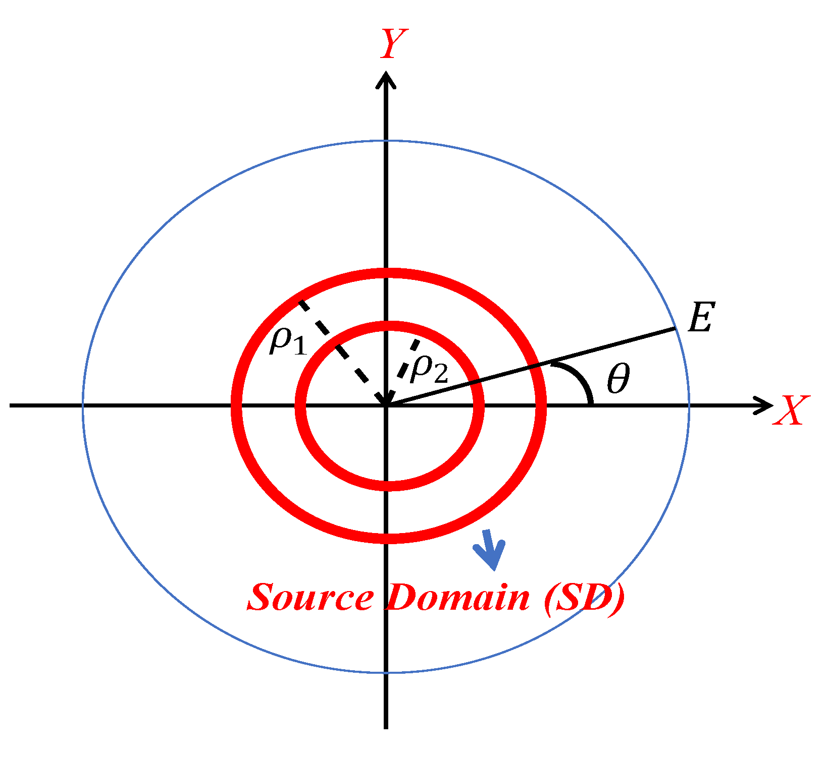
Let us consider two circumferences sources, as shown in Figure 1. The geometry is a z-invariant electric current source =, where means transpose, defined on each circumference, where and are the radius of the inner and outer circumference, respectively, and are the angular variable on each circumference. The source is embedded in a homogeneous medium with the free-space dielectric permittivity () and magnetic permeability ().
At a single frequency, the total electric far-field in the angular source sector can be provided by the linear integral operator.
where
and
The wavenumber is , and and denote the angular frequency and the wavelength, respectively.
Since the operator (1) is linear and compact, the SVD can be defined for each source geometry and consists of the triple [23], where and are the singular functions, and is the n-th singular value. In Appendix A, it is shown that the exponentially vanish when , where stands for the nearest integer and because of the asymptotic behavior of the Bessel functions for orders much larger than arguments. Consequently, the closed-form NDF can be achieved by as the number of significant singular values for a stable inversion [24].
The adjoint operator of (1) can also be defined to find the solution to the inverse problem as , where we have the following:
The PSF is now considered to evaluate the performance of the reconstruction algorithm. The PSF analysis is used in the inverse source problem to determine how the source geometry and observation domain affect the resolution. Here, we intend to analyze only the influence of the source geometry. The final goal is to obtain an analytical estimation of the achievable resolution and link it to geometrical parameters.
The PSF of our interest is provided by the current distribution in the source domain for a point source located at . It is defined mathematically as the impulsive response of the system provided by the cascade operator , as follows:
where is the regularized inverse operator of , is the Dirac delta function, and can be either 1 or 2.
The PSF is given by the completeness relation truncated to the singular functions with non-zero singular values because the minimum–norm solution of the inverse source problem is a projection of the actual source onto the singular function with non-zero singular values. Thus, the PSF is dependent on the number of retained singular values, i.e., the NDF. Based on the SVD properties, the actual closed-form PSF function (see Appendix A) is analytically provided by (A9).
Now the approximated PSF is introduced as follows. From the spectral theorem for compact self-adjoint operators applied to the cascade , we can compute the following:
whose kernel is as follows:
Finally, by substituting Equations (7) to (6), it reads as follows:
where is the zeroth-order Bessel function of the first kind.
Now, a general strategy to build a good approximation of the PSF concerns the approximation of the inverse operator in Equation (5) by the adjoint one [19,25,26]. This happens when the singular values of the pertinent operator exhibit a nearly constant behavior before the knee of their curve. As a result, we define the approximated as follows:
Therefore, Equation (8) provides the analytical evaluation of (9) for the geometry under consideration.
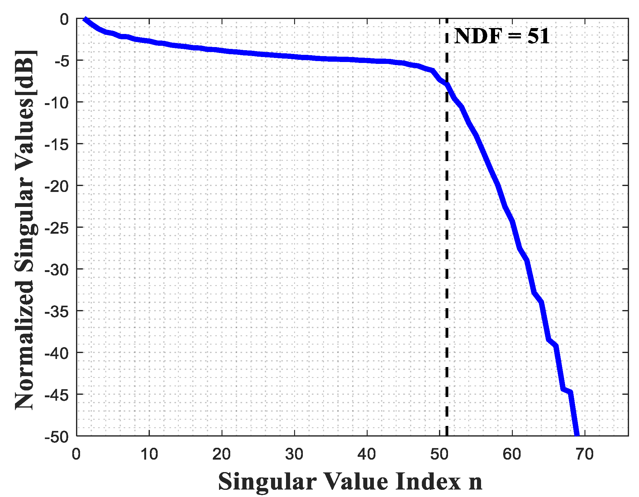
We now provide some numerical simulations to examine the results of the above-mentioned exact and analytical evaluations of the PSF. In this way, we can also investigate how adding an inner circumference inside an outer circumference affects the NDF, and whether it is possible to reconstruct the inner source or not. We addressed the same analysis to evaluate the NDF for two square sources in Ref. [27]. It has been shown that increasing the size of the inner square has no noticeable effect on singular value behavior, and regardless of how small the inner square is, the behavior of singular values in the outer square would be similar to that of two squares. Thus, it can be confirmed that the inner source cannot add the NDF by considering a comparison of different sizes of the inner source.
Let us consider the geometry of Figure 1, for and different values of . The upper bound of the NDF is 51. Figure 2 shows that changing the size of the inner source can affect the behavior of singular values only slightly; however, as expected by the result of Appendix A, the NDF does not change. It can be concluded that the contribution of the inner circumference is negligible, and it is possible to ignore it to achieve the whole NDF. Furthermore, it is difficult to understand whether the inner source is present or not, and it may be impossible to reconstruct it. This problem is still challenging in inverse source problems, and maybe it can be reconstructed by using more prior information about it.
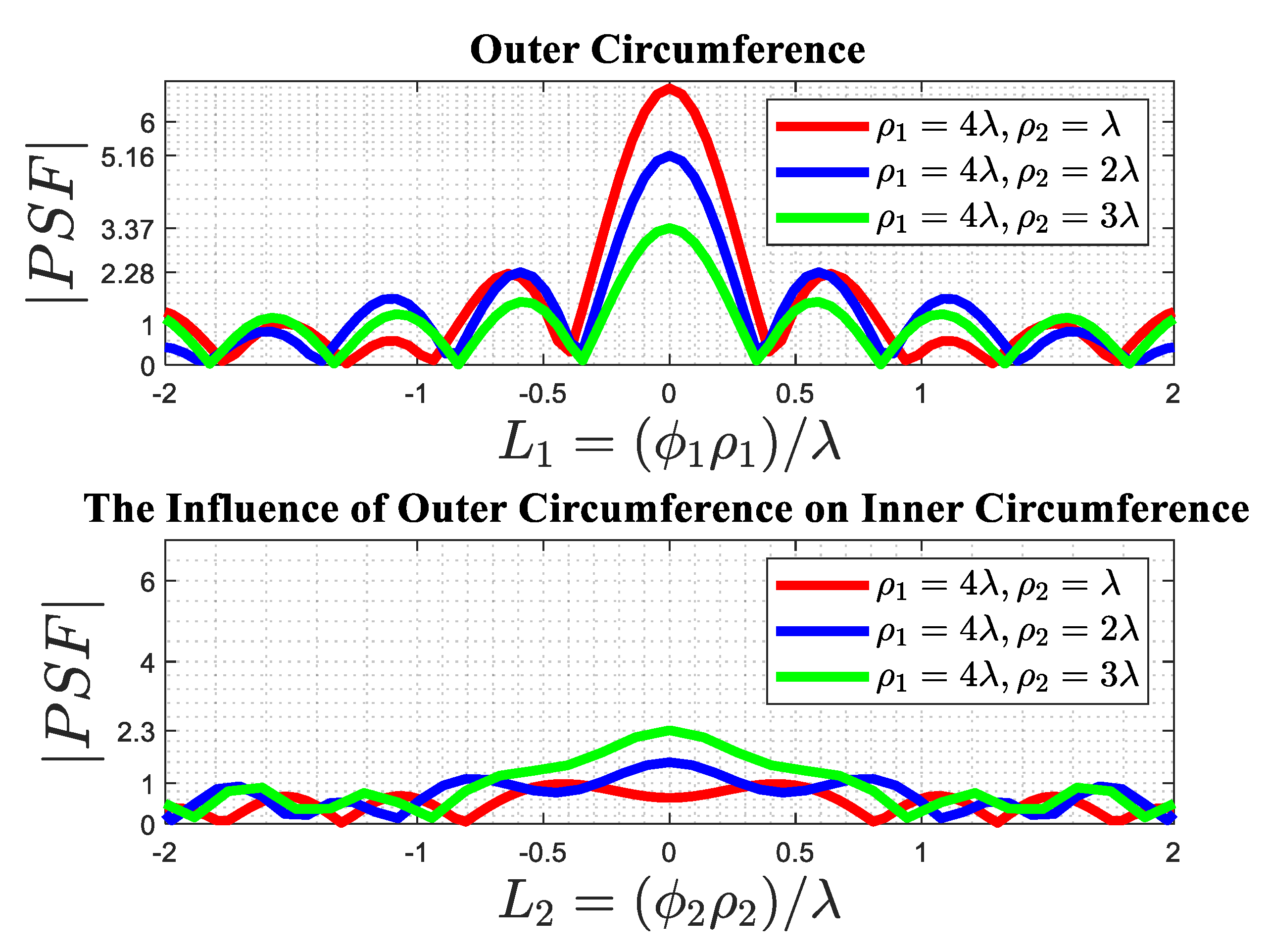
Next, the behavior of the analytical PSF is verified. Since the PSF is a function only of it can be arbitrarily selected the point source locations in the source domain: it is the angularly invariant function; that is all point-like sources can be imaged in the same way, independent of their positions. Figure 3 shows the actual PSF of the outer circumference and its influence on the inner circumference for a point-like source located at . Generally, the resolution result is evaluated by the Full-Width Half Maximum (FWHM) criterion. The result confirms that the resolution is equal to in the inverse source problem. In addition, the PSF result of the outer circumference cannot significantly affect the inner one.
It can be observed that increasing the size of the inner source can reduce the amplitude of the PSF of the outer source; in addition, the amplitude of its influence on the inner rises, but the resolution remains unchanged. This means that, when it is known in advance that the source is composed of two circumferences, it can be expected that, for spacing smaller than , the resolution along the radius is about .
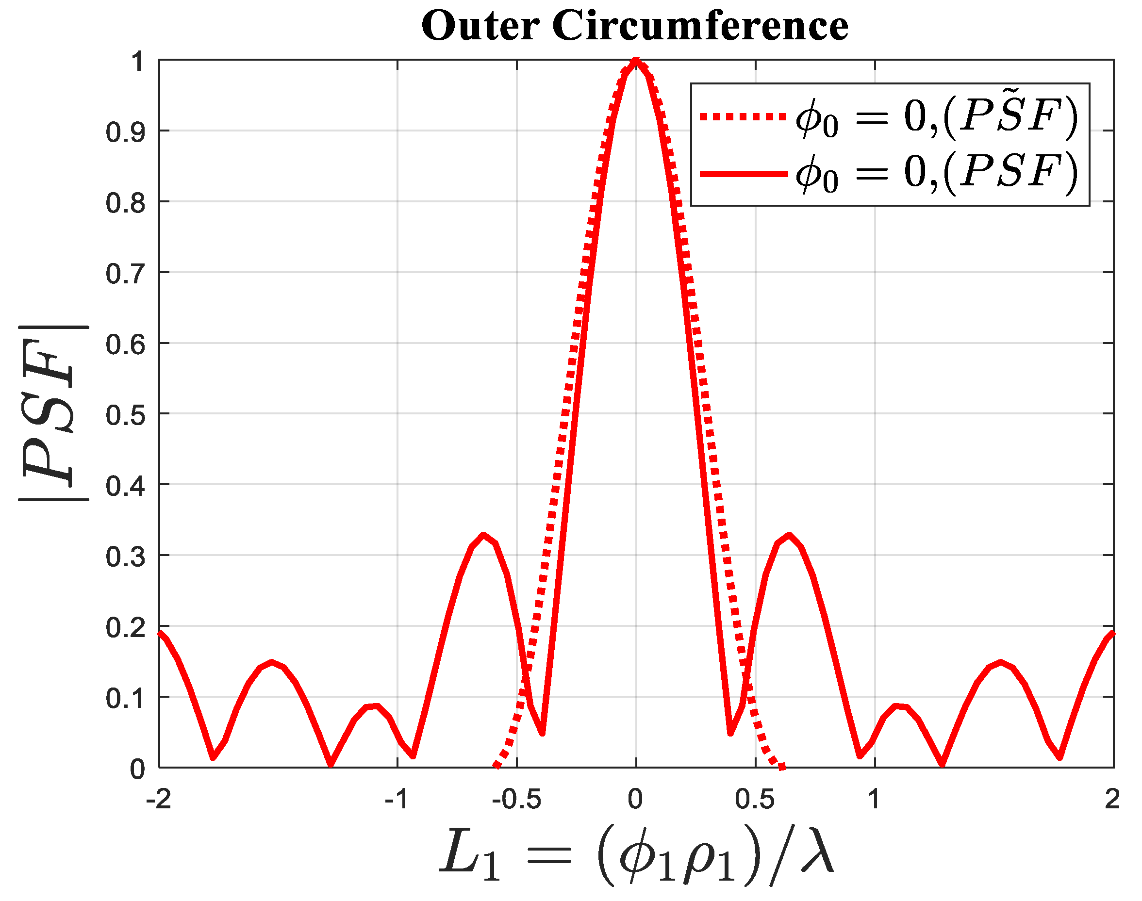
Finally, a comparison between the approximated and the actual PSF is provided in Figure 4. The amplitude of both PSF normalized to 1. It is confirmed that, in the main lobe region, the closed-form approximation is acceptable.
3. The Inverse Scattering Problem
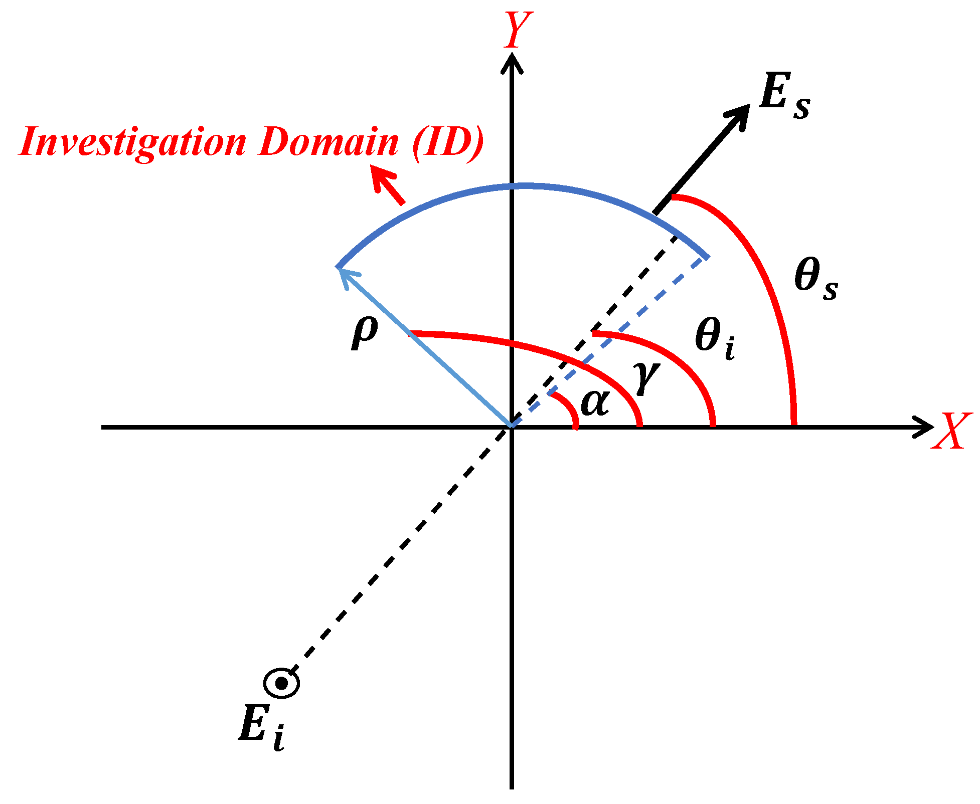
In this section, we address the analysis of the PSF in inverse scattering problem as in Section 2; additionally, the NDF of an arc of the circumference is provided analytically. Let us consider a dielectric scatterer, with as relative permittivity, belonging to a domain referred to as the investigation domain (ID), which is located in a homogenous background, with the free-space permittivity, , and illuminated by incident plane waves from different angles. Figure 5 depicts the general circumference geometry of the problem. The direction of plane wave and direction of observation is denoted by and , respectively. For each incident plane wave, the scattered field is observed in the far zone; and are the extremal angles of the scatterer, respectively, and is the radius of the arc of circumference.
Hence, for the forward problem, the scattered far-field () under the Born approximation is provided by the following:
where is the contrast function. Now, since is a linear and compact operator for the multi-view and single frequency scattering configurations of our present interest, the SVD can be applied to evaluate the NDF in terms of the pertinent singular values and the PSF in terms of the corresponding singular functions.
Since it is difficult to find an explicit expression of the SVD of (10), in order to provide some clues about it, we apply the method proposed in Ref. [28] to estimate the NDF of an arc source to present the scattering problem. First, we rewrite Equation (10) as follows:
Then we expand the contrast function under a Fourier series as and to examine the contribution that each of the contrast harmonics can provide to the scattered field.
Next, by exploiting the Jacobi-Anger expansion [29] and the orthogonal property of the exponential functions over the interval [0, 2π], we compute the scattered field by one of harmonics as follows:
consequently resulting in a double Fourier series, where and . Now, the expansion coefficients peak at the order , because of the sinc function dependence, and, because of the exponential decay of the Bessel functions for arguments much larger than the order, the maximum order is . Since , then . Accordingly, the maximum number of Fourier harmonics of the contrast function that can provide a contribution to the scattered field is . This also provides the upper bound of the NDF of (10).
In an inverse scattering problem, the scattered fields for all plane waves are observed, and then the task is to reconstruct the contrast function. In order to solve the inverse scattering problem, the adjoint operator of (10) can be helpful, and it is defined as follows:
From the spectral theorem for compact self-adjoint operators applied to , it follows that
whose kernel is as follows:
is provided by the square of the Bessel function of the first kind and zeroth order. Finally, substituting Equations (15) to (14) results as follows:
The PSF analysis is used in the inverse scattering problem to determine how the scatterer geometry and observation domain may influence the resolution. Only the effect of scatterer geometry on the resolution is considered here. The reconstruction of a point-like scatterer is provided by the PSF. As pointed out in Section 2, when the PSFs for the inverse source problem have been introduced, the adjoint operator can be used to approximate the inverse operator and hence an approximated can be introduced as well, in Section 2, by replacing and with and , respectively, in Equations (5) and (9).
3.1. Two Circumferences
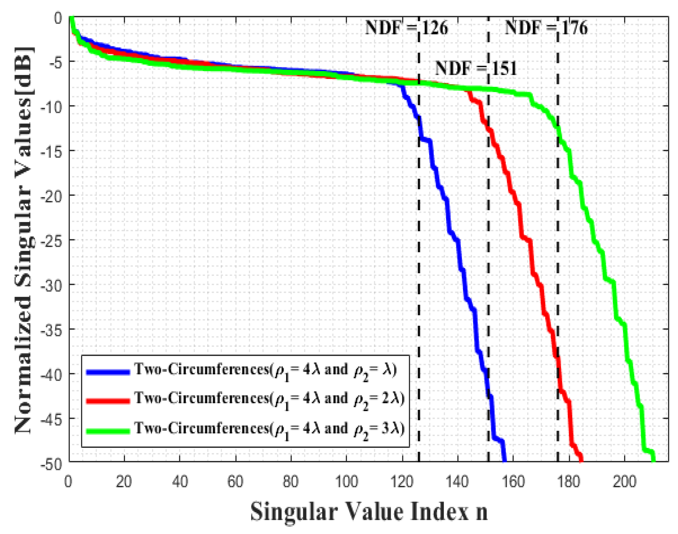
This subsection considers two circumferences to show the difference between this case and the considered geometry in the inverse source problem. As in Section 2, we consider different sizes of inner circumference.
First of all, we consider the NDF of this geometry and follow the same approach as in (1) to define a block operator accounting for more than one scattering object. Following the same reasoning of Refs. [27,30,31], if the distance between two scatterers is sufficiently large, the kernel norms and, consequently, the operator norms for the diagonal contributions of the pertinent operator are expected larger than for the off-diagonal ones. Therefore, the operator becomes a diagonal block operator, and its eigenvalues are the combination of each block. This result implies that the whole functional space of the scattered far fields can be approximately decomposed under two individual orthogonal subspaces. Thus, the NDF of an arbitrary number of scattered fields can be given as follows:
and the total NDF can be obtained approximately by summing the and of each scatterer.
The implication of the increase of the NDF for the inverse scattering problem compared to the inverse source problem for the same geometry concerns the possibility of reconstructing a point-like scatterer lying on the inner circumference. As mentioned before, inserting another circumference source inside the outer circumference source cannot increase the NDF; on the other hand, the NDF will be increased in the inverse scattering problem. Furthermore, it is impossible to reconstruct the inner circumference source in the inverse source problem, whereas the inner circumference object can be reconstructed in the inverse scattering problem. To this end, some numerical simulations will be presented.
The behavior of normalized singular values of the relevant operator is plotted in Figure 6. The characteristic of the two circumferences are , , , and the different sizes of , where the index 1 and 2 indicate the outer and the inner circumference, respectively. It can be seen that the total NDF is achieved approximately by summing the NDF of two circumferences. The NDF is varied by changing the radius of the inner circumference compared to the inverse source problem. For reference, we just choose a sufficiently large number of plane waves to ensure to achieve all the predicted NDF so that the number of plane waves for this simulation is 60.
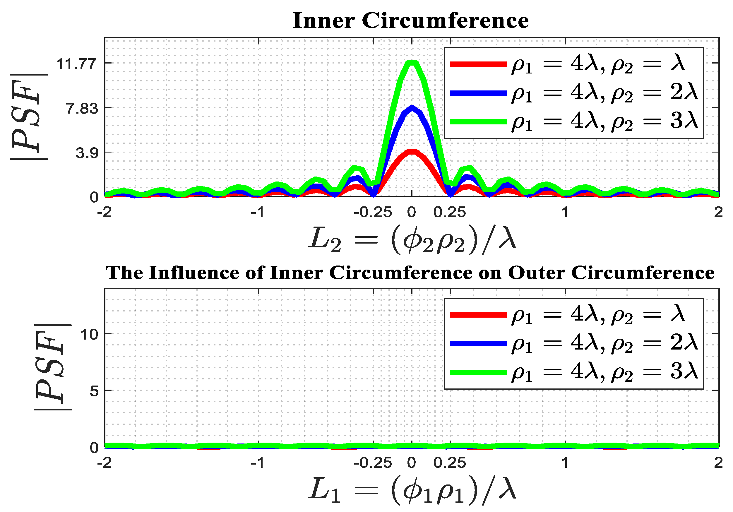
Figure 7 shows the actual PSF of the outer circumference and its influence on the inner one for a point scatterer located at . The actual PSF is numerically computed by a custom numerical code run in MATLAB environment by discretization of the relevant operator over a sufficiently fine grid. The FWHM criterion evaluates the achievable resolution result. The result confirms that the achievable resolution is . As can be observed, the amplitude of the main lobe of the outer circumference does not change when the radius of the inner varies. Furthermore, the PSF of the outer circumference cannot influence the inner.
The actual PSF of the inner circumference and its influence on the outer circumference for a point-like scatterer located at is plotted in Figure 8. It can be observed that the amplitude of the main lobe of the inner circumference varies when the radius of the inner changes. The amplitude of the main lobes of the inner circumference is larger than the amplitude of the side lobes of the outer circumference in Figure 7. The PSF of the inner circumference cannot affect the outer one. Consequently, it is possible to reconstruct the inner circumference, and a point-like scatterer can be distinguished lying either on it or on the outer one.
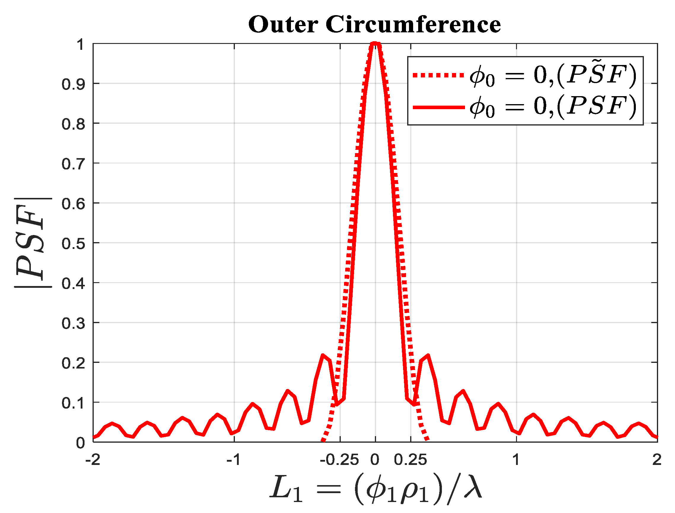
Next, a comparison between the actual PSF and the approximated one is provided to appreciate the accuracy of the approximated PSF. Figure 9 confirms that the main lobes of approximated (dotted red curve) and the actual PSF (solid red curve) are nearly overlapped. It means that the approximation is very accurate at estimating the achievable resolution that can be achieved.
3.2. Two Arcs of Circumferences
In this subsection, in order to provide a more general example, we address the case of two arcs of two different circumferences. The geometry of this problem is depicted in Figure 5 so that , , and , and . The aim is twofold: to confirm that the whole NDF is approximately equivalent to the summation of the NDF of each scatterer and to appreciate the validity of the approximation of the PSF for resolution purposes.
Figure 10 shows the behavior of normalized singular values of the relevant operator with 60 plane waves. The upper bound NDF of the two scatterers is 51. The result proves that the total NDF is approximately achieved by summing the NDF of two scatterers.
The next numerical simulation refers to the influence of the actual PSF of the arc of circumference 1 on the other one. The considered point positions are , and and the corresponding PSFs results are shown in Figure 11. In this way, we can appreciate how imaging performance remains constant when the position of the point scatterer changes. In fact, if the location of the point scatterer changes, the width of the main lobe does not change, which means the resolution remains constant. Furthermore, the PSF of scatterer 2 cannot affect the other one.
A numerical simulation is presented to show the influence of the actual PSF of scatterer 2 on the other. The position of the considered points are , and and the corresponding PSFs results are displayed in Figure 12. Again, we observed that the width of the main lobes does not vary when the position of the point scatterers changes. It indicates that the PSF is space invariant, which means that the resolution of a point-like scatterer is independent of its location.
The same simulation as in the previous subsection is here provided to compare the results of the relevant PSF and the for different positions of . As demonstrated in Figure 13, the main lobes of the approximated (dotted lines) are approximately overlapped with the actual PSF (solid lines).
It can be concluded that in the inverse source and inverse scattering problem, when the observation domain is between and , while the PSF maximum value may depend on the point source/scatterer, the width of its main lobe does not change and is independent of the position of the point source/scatterer. Since the resolution of a point-like source/scatterer is limited by the width of the PSF, it is the same over the whole source/investigation domain.
4. Optimal Number of Incident Plane Waves
In the previous section, we performed an NDF analysis of the field scattered by circumference geometries under plane wave incidence. It was assumed that a sufficiently high number of waves impinge on the object so that the NDF is achieved. In inverse scattering problems, the scattered field data can be acquired by changing either the observation direction or the direction of the impinging plane wave. The knowledge of the NDF of the linearized scattering operator cannot provide any clue about how to discretize the scattered field data optimally. Therefore, from the theoretical point of view, two questions arise when multiple plane waves are used to achieve the NDF: The first one is, how many independent plane waves are needed? The second one is, which directions of plane waves are the optimal ones, in the sense that they allow us to achieve the total NDF of the operator? In the absence of theoretical arguments, we choose to investigate numerically only the question of the minimum number of impinging plane waves that can be significant in achieving the total NDF. An answer to this point can be valuable in decreasing the cost of imaging systems, as for instance, in radar imaging, since it allows us to reduce the number of transmitters (and receivers) to a minimum.
In principle, increasing the number of independent plane waves can increase the NDF, namely the number of significant singular values of the operator; after that, it can only affect their behavior in the decaying region. Generally, finding the exact optimal number and its direction for each geometry is complicated because they are dependent on the geometry of the problem, i.e., the number of the scatterers, the distance between them, their location, size, and shape. It means that it is difficult to introduce a general rule for every geometry, and it cannot be predicted easily how many independent plane waves are enough and which directions are the best.
To this end, the reciprocity theorem might be helpful, as the inverse scattering problem reduces to an inverse source problem for a single plane wave incidence. According to it, the far-field scattered along a direction for a plane wave impinging on the direction is the same when we consider a plane wave impinging on and observe the far-field at the direction . Therefore, if we call the NDF of the corresponding inverse source problem, it would result from for the pertinent inverse scattering problem and NDF, and plane waves would be needed, as each individual one might add pieces of information to the total scattered field. While this reasoning can provide an upper bound about the NDF and the number and directions of the independent plane waves, the actual number is lower.
Likewise, in Ref. [31], we have analyzed the same problem for strip geometries in and variable. It has been shown that two incident plane waves for two strips and four incident plane waves for the cross-strip are adequate for achieving all NDF of these scattering geometries. Moreover, optimum directions of the plane waves for each geometry were introduced. It was proved that the same NDF could be achieved independently on the observation variable, and the only difference is the behavior of singular values.
The purpose of this section is to investigate the minimum number of independent plane waves for the considered geometries to achieve the whole NDF, as well as to introduce the optimal directions of plane waves. To this end, a comparison between different numbers of plane waves for each geometry is presented. Since, at the moment, it is difficult to introduce a closed-form rule to define the optimal number and its direction, we provide them numerically.
We first consider an arc of a circumference that its radius is equal to , and . Figure 14 illustrates the behavior of the singular value of the relevant operator for different numbers of plane waves. For reference, we just choose a sufficiently large number of plane waves to ensure to achieve all the predicted NDF.
As can be observed in Figure 14, the NDF is added by increasing the number of plane waves; however, the NDF will not add after two plane waves (purple line), and the behavior of the singular values can only change within the decay region. Overall, it can be seen that the NDF can be approximately achieved by considering only two plane waves, which are and . It must be noticed that finding the optimal number is dependent on the size of the circumference, which means that, if its size increases, the optimal number of the plane wave will increase. However, two plane waves are only adequate for this geometry. This result agrees with Ref. [31], as this circumference geometry is not far from a rectilinear one.
The second numerical simulation is the same as the first one to represent the behavior of the normalized singular values for two arcs of two different circumferences at various numbers of incident plane waves from different directions, as shown in Figure 15. The result shows again that the NDF increases by increasing the number of plane waves from one to two (purple line) plane waves; only the behavior of the singular values varies beyond two. The direction of two plane waves is . It can be observed that when we consider three plane waves with , the total NDF is achieved as well. Consequently, the optimal direction of the plane waves depends on the scattering geometry compared with the previous simulation.
The third simulation is devoted to considering one circumference whose radius is equal to . Figure 16 shows the behavior of the singular value of the relevant operator for different numbers of plane waves. It can be viewed that increasing the number of plane waves can increase the NDF; however, the NDF will not increase after four plane waves (red line), and the behavior of the singular values can only change. Overall, the NDF can be approximately achieved by considering only four plane waves, which are , , , and .
The fourth numerical simulation concerns the behavior of the normalized singular values for two different circumferences, which the radius of the outer and inner are equal to and , respectively, as shown in Figure 17. As can be illustrated, the NDF is added by increasing the number of plane waves; however, the NDF will not add after four plane waves (green line), and the behavior of the singular values can only change. Thus, four plane waves are approximately adequate because the exponential decay of the singular values is met approximately at the same point compared to six and 60 plane waves, although the only difference is the behavior of their singular values. The directions of the four plane waves are .
In conclusion, the numerical simulations confirm that finding the optimal number of the plane waves and their directions are dependent on the size of the scatterer, the number of the scatterer, their shapes, and their locations. Therefore, it may be difficult to find a general rule.
5. A Numerical Application in Inverse Scattering
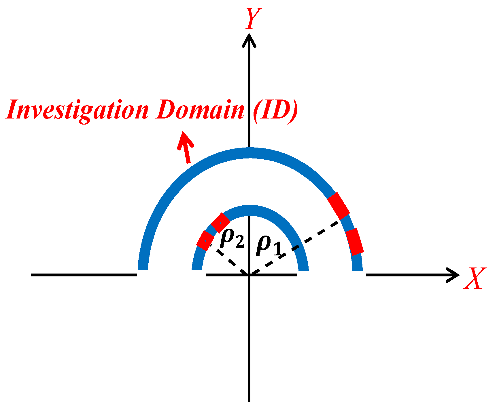
This section aims at showing the practical relevance of the above theoretical discussions by the numerical reconstruction of an object dielectric located in free space. It consists of two dielectric semi-circumference strips with , and the width 0.4λ, as illustrated in Figure 18, and the contrast is .
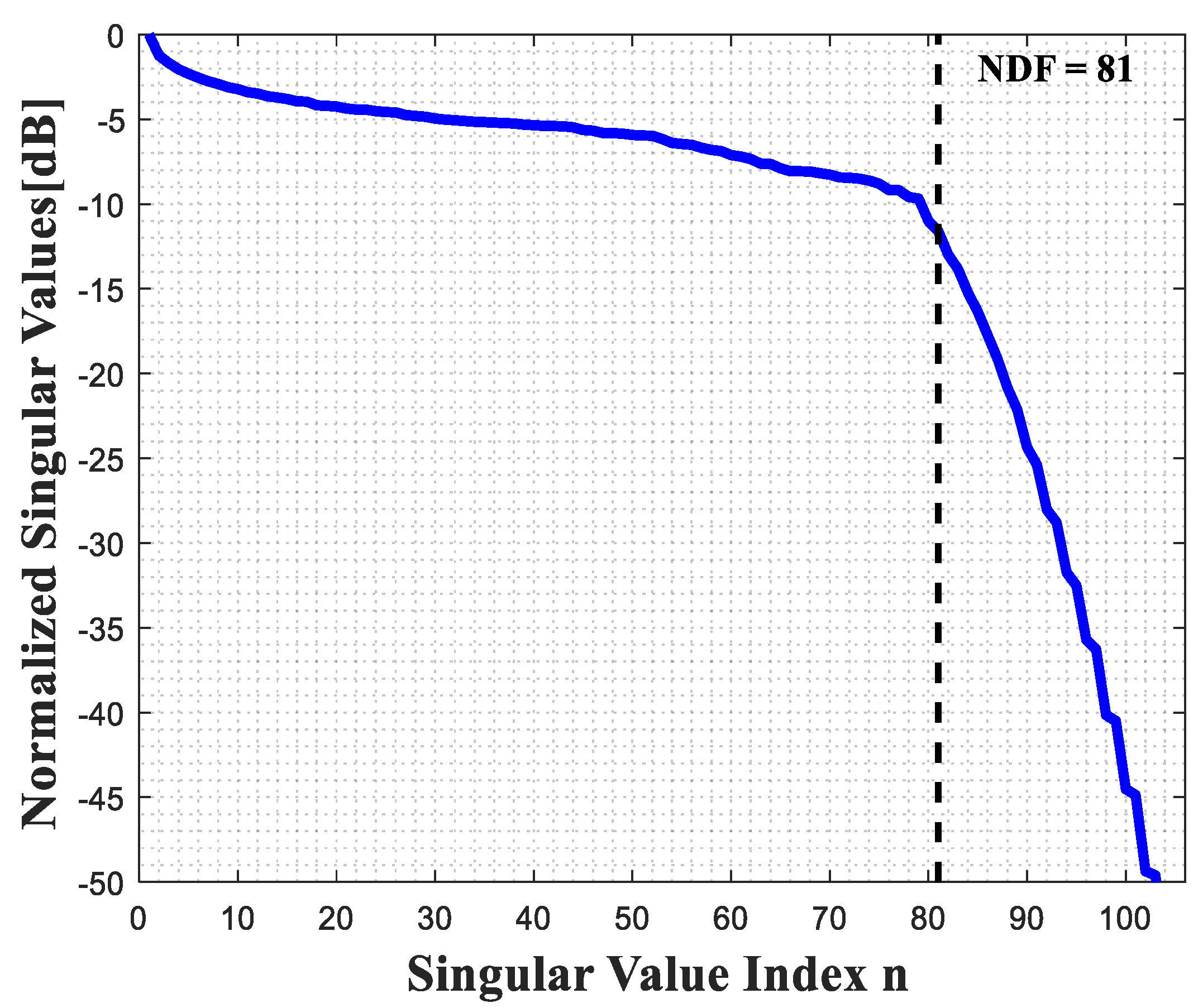
Then, we assume that two cracks (free space condition, ) exist in the outer semi-circumference, and two cracks are present in the inner semi-circumference. In the outer semi-circumference, the width of each crack and the distance between them is ; the length of each crack and the distance between them is in the inner semi-circumference. All the simulation parameters are the same as in the previous section. The normalized singular values of the related operator is plotted in Figure 19 to compute the NDF. For this simulation, the number of plane waves is 60, and the expected NDF is 81.
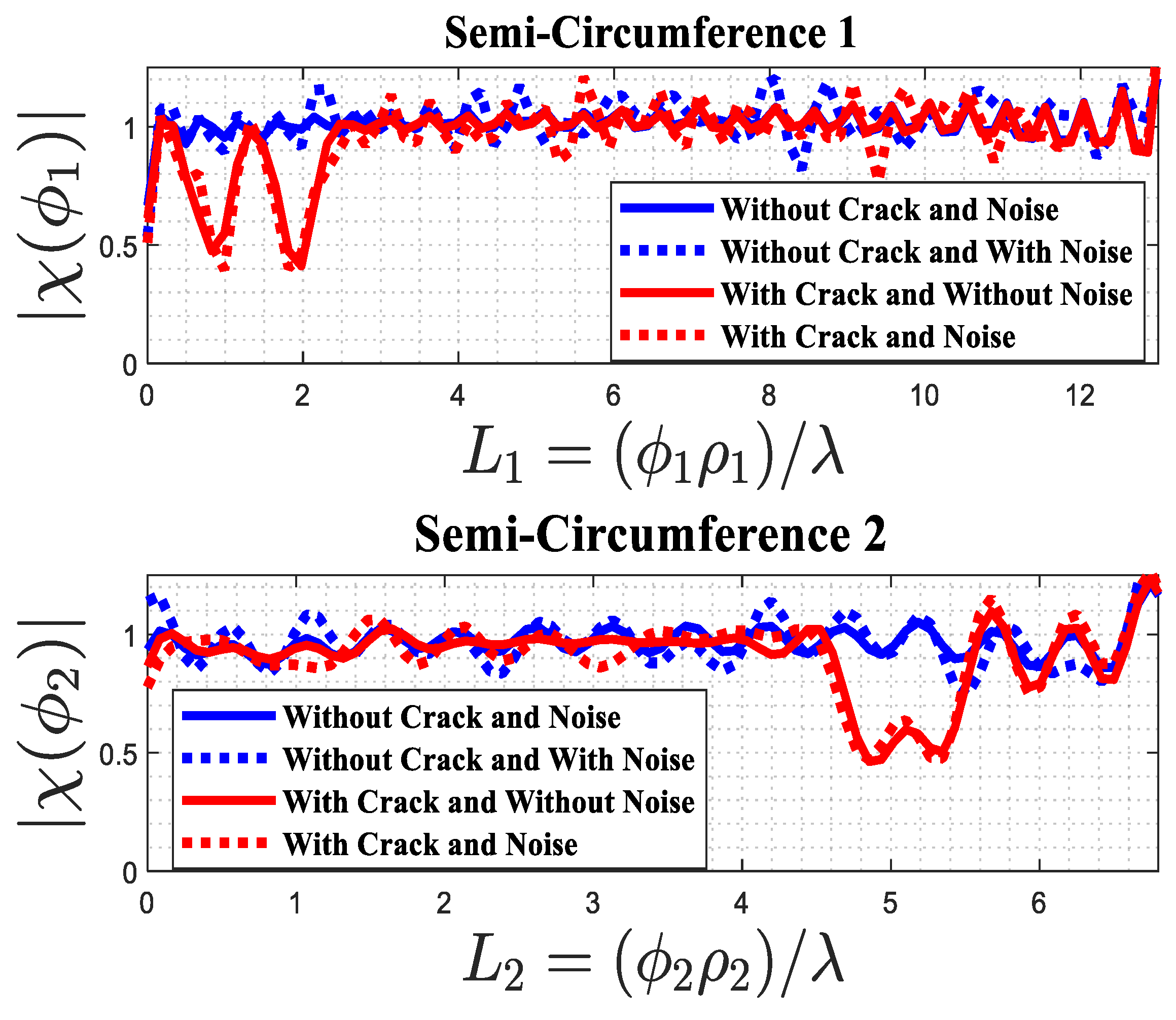
It must be noted that the mathematical procedure of the reconstruction algorithm is significant to solve the problem. Since all actual scattered fields always include noise, the reconstructed image may also be noisy, and the cracks may not be detected. Therefore, it is crucial that the inversion algorithm can mitigate the noise effect. To this end, the Truncated SVD algorithm is adopted to reconstruct the contrast function, and we fix the threshold value to include the first NDF singular values. Then additive white Gaussian noise is added to the simulated scattered field, with a noise level such that the Signal-to-Noise Ratio (SNR) is 10 dB, and results are shown in Figure 20.
As can be observed, it can be distinguished that two cracks are present along the outer semi-circumference; oppositely, it is impossible to differentiate between two cracks in the inner semi-circumference. It is important to note that the two cracks separated by the distance can be resolved well also in the presence of noise on data. Hence, the resolution analysis is important for the reliable reconstruction of defects in dielectric objects in inverse scattering problems.
6. Conclusions
We have investigated the role of the NDF and the PSF in the linear electromagnetic inverse for both source and scattering problems to estimate the achievable resolution. Since the results may depend on the geometry, we have taken into consideration one different from Ref. [19], that is, the circumference one. The PSF can be implemented by the numerical solution of the relevant inverse problem. Since finding the exact evaluation of the PSF is complicated and can only be performed numerically for most geometries, an approximate analytical assessment was introduced, and its accuracy was assessed against the actual PSF for each geometry by numerical simulations. In addition, the closed-form evaluation of the PSF in inverse source and the analysis of the closed-form NDF in inverse scattering were provided. Two circumferences were addressed to prove that the inner source is negligible to achieve the NDF and cannot add the NDF; conversely, the inner circumference can increase the NDF in inverse scattering.
We have demonstrated that, when the observation domain scans the full angle in the far zone region, space invariant PSF is achieved, which means that the maximum resolution of the reconstruction of point-like sources/objects is obtained independently of their locations within the investigation domain, and the resolution remains unchanged. Specifically, the achievable resolutions for considered geometries are and for the inverse source and scattering problems, respectively, as in Ref. [19]. Furthermore, we have shown that increasing the number of independent plane waves can add the NDF until the minimum number of plane waves that are needed to achieve the whole NDF; thus, the optimal number of independent plane waves and their direction was introduced numerically. The result illustrated that finding optimal number and their direction is dependent on the characteristics of the scatterer, such as its size and the number of the scatterer. In Section 5, the numerical example has shown the relevance of the approach to microwave tomography of dielectric objects, and when noise is present, the two cracks separated by the distance can be reconstructed well.
Author Contributions
Conceptualization, G.L. and R.P.; methodology, G.L. and R.P.; software, E.A.S.; validation, E.A.S. and G.L.; formal analysis, E.A.S. and G.L.; investigation, E.A.S. and G.L.; resources, E.A.S.; data curation, E.A.S.; writing—original draft preparation, E.A.S.; writing—review and editing, G.L.; visualization, G.L.; supervision, R.P.; project administration, G.L.; funding acquisition, R.P. All authors have read and agreed to the published version of the manuscript.
Funding
This research received no external funding.
Data Availability Statement
Data supporting reported results are generated during the study.
Conflicts of Interest
The authors declare no conflict of interest.
Appendix A
In this appendix, we derive the singular system of the operator (1) to compute the closed-form of the PSF in inverse source problems. For a circle source, the singular system is readily provided in the closed-form [29] by the following:
where is the n-th Bessel function of the first kind.
As is well-known, the singular functions and the singular values of the operator satisfy the equations , and (see (2)). Therefore, the following two eigenvalue problems arise: , and . We start considering the latter one and evaluate the following:
By exploiting the Jacobi–Anger expansion [29] and the orthogonal property of the exponential in θ; over the interval [0, 2π], (A2) becomes the following:
Therefore, the following is apparent:
It is possible to show that decay exponentially for , where stands for the nearest integer and . Now, we consider the following equation to compute the singular functions:
Then we get the following:
By substituting Equation (A6) to (A5), it follows that we get the following:
Then the singular functions are given by the following:
Finally, the closed-form PSF is given by the following:
which holds both for and .
References
- Buzug, T.M. Computed tomography. In Springer Handbook of Medical Technology; Springer: Berlin/Heidelberg, Germany, 2011; pp. 311–342. [Google Scholar]
- Piestun, R.; Miller, D.A. Electromagnetic degrees of freedom of an optical system. J. Opt. Soc. Am. A Opt. Image Sci. Vis. 2000, 17, 892–902. [Google Scholar] [CrossRef] [PubMed]
- Miller, D.A.B. Communicating with waves between volumes: Evaluating orthogonal spatial channels and limits on coupling strengths. Appl. Opt. 2000, 39, 1681–1699. [Google Scholar] [CrossRef] [PubMed] [Green Version]
- Toraldo di Francia, G. Degrees of Freedom of an Image. J. Opt. Soc. Am. 1969, 59, 799–804. [Google Scholar] [CrossRef]
- Bendinelli, M.; Consortini, A.; Ronchi, L.; Frieden, B.R. Degrees of freedom, and eigenfunctions, for the noisy image. J. Opt. Soc. Am. 1974, 64, 1498–1502. [Google Scholar] [CrossRef]
- Solimene, R.; Pierri, R. Number of degrees of freedom of the radiated field over multiple bounded domains. Opt. Soc. Am. 2007, 32, 3113–3115. [Google Scholar] [CrossRef]
- Solimene, R.; Maisto, M.A.; Pierri, R. Inverse source in the near field: The case of a strip current. J. Opt. Soc. Am. A 2018, 35, 755–763. [Google Scholar] [CrossRef] [PubMed]
- Pierri, R.; Moretta, R. Asymptotic Study of the Radiation Operator for the Strip Current in Near Zone. Electronic 2020, 9, 911. [Google Scholar] [CrossRef]
- Bucci, O.M.; Franceschetti, G. On the degrees of freedom of scattered fields. IEEE Trans. Antennas Propag. 1989, 37, 918–926. [Google Scholar] [CrossRef]
- Bertero, M.; Viano, G.A.; Pasqualetti, F.; Ronchi, L.; Di Francia, G.T. The Inverse Scattering Problem in the Born Approximation and the Number of Degrees of Freedom. Opt. Acta Int. J. Opt. 1980, 27, 1011–1024. [Google Scholar] [CrossRef]
- Brancaccio, A.; Leone, G.; Pierri, R. Information content of Born scattered fields: Results in the circular cylindrical case. J. Opt. Soc. Am. A 1998, 15, 1909–1917. [Google Scholar] [CrossRef]
- Solimene, R.; Maisto, M.A.; Pierri, R. Inverse scattering in the presence of a reflecting plane for the strip case. J. Opt. 2015, 18, 025603. [Google Scholar] [CrossRef]
- Rihaczek, A.W. Radar resolution of ideal point scatterers. IEEE Trans. Aerosp. Electron. Syst. 1996, 32, 842–845. [Google Scholar] [CrossRef]
- Solimene, R.; Leone, G.; Pierri, R. Resolution in two-dimensional tomographic reconstructions in the Fresnel zone from Born scattered fields. J. Opt. A Pure Appl. Opt. 2004, 6, 529. [Google Scholar] [CrossRef]
- Mensa, D.L. High Resolution Radar Cross-Section Imaging; Artech House: Boston, MA, USA, 1991. [Google Scholar]
- Schnattinger, G.; Eibert, T.F. Dyadic Point Spread Functions for 3D Inverse Source Imaging Based on Analytical Integral Solutions. Prog. Electromagn. Res. 2014, 58, 1–17. [Google Scholar] [CrossRef] [Green Version]
- Majumder, U.K.; Temple, M.A.; Minardi, M.J.; Zelnio, E.G. Point spread function characterization of a radially displaced scatterer using circular synthetic aperture radar. In Proceedings of the 2007 IEEE Radar Conference, Waltham, MA, USA, 17–20 April 2007. [Google Scholar]
- Maisto, M.A.; Solimene, R.; Pierri, R. Resolution limits in inverse source problem for strip currents not in Fresnel zone. JOSA A 2019, 36, 826–833. [Google Scholar] [CrossRef] [PubMed]
- Sekehravani, E.; Leone, G.; Pierri, R. PSF Analysis of the Inverse Source and Scattering Problems for Strip Geometries. Electronics 2021, 10, 754. [Google Scholar] [CrossRef]
- Leone, G.; Maisto, M.A.; Pierri, R. Inverse Source of Circumference Geometries: SVD Investigation based on Fourier Analysis. Prog. Electromagn. Res. M 2018, 76, 217–230. [Google Scholar] [CrossRef] [Green Version]
- Leone, G.; Munno, F.; Pierri, R. Inverse Source on Conformal Conic Geometries. IEEE Trans. Antennas Propag. 2021, 69, 1596–1609. [Google Scholar] [CrossRef]
- Leone, G.; Munno, F.; Pierri, R. Radiation of a Circular Arc Source in a Limited Angle for Non-uniform Conformal Arrays. IEEE Trans. Antennas Propag. 2021, 69, 4955–4966. [Google Scholar] [CrossRef]
- Bertero, M.; Boccacci, P.P. Introduction to Inverse Problems in Imaging; IOP Publishing: Bristol, UK, 1998. [Google Scholar]
- Leone, G. Source geometry optimization for hemispherical radiation pattern coverage. IEEE Trans. Antennas Propag. 2016, 64, 2033–2038. [Google Scholar] [CrossRef]
- Pierri, R.; Liseno, A.; Soldovieri, F.; Solimene, R. In-depth resolution for a strip source in the Fresnel zone. J. Opt. Soc. Am. A Opt. Image Sci. Vis. 2001, 18, 352–359. [Google Scholar] [CrossRef] [PubMed]
- Solimene, R.; Maisto, M.A.; Pierri, R. Sampling approach for singular system computation of a radiation operator. J. Opt. Soc. Am. A Opt. Image Sci. Vis. 2019, 36, 353–361. [Google Scholar] [CrossRef] [PubMed]
- Sekehravani, E.A.; Leone, G.; Pierri, R. NDF of the far zone field radiated by square sources. In Proceedings of the XXXIVth General Assembly and Scientific Symposium of the International Union of Radio Science, Rome, Italy, 28 August–4 September 2021. [Google Scholar]
- Leone, G.; Maisto, M.A.; Pierri, R. Application of Inverse Source Reconstruction to Conformal Antennas Synthesis. IEEE Trans. Antennas Propag. 2018, 66, 1436–1445. [Google Scholar] [CrossRef]
- Devaney, A.J. Mathematical Foundations of Imaging, Tomography and Wavefield Inversion; Cambridge University Press: Cambridge, UK, 2012. [Google Scholar]
- Leone, G.; Munno, F.; Pierri, R. Synthesis of Angle Arrays by the NDF of the Radiation Integral. IEEE Trans. Antennas Propag. 2020, 69, 2092–2102. [Google Scholar] [CrossRef]
- Sekehravani, E.A.; Leone, G.; Pierri, R. NDF of Scattered Fields for Strip Geometries. Electronics 2021, 10, 202. [Google Scholar] [CrossRef]
Figure 1.
The geometry of the problem.

Figure 2.
Comparison of the behavior of the normalized singular values of the relevant operator of the inverse source problem for one and two circumferences cases.
Figure 2.
Comparison of the behavior of the normalized singular values of the relevant operator of the inverse source problem for one and two circumferences cases.

Figure 3.
The Point Spread Function (PSF) of the outer circumference and its effectiveness on the inner one.
Figure 3.
The Point Spread Function (PSF) of the outer circumference and its effectiveness on the inner one.

Figure 4.
Comparison of normalized amplitude of the actual PSF and the approximated PSF for .

Figure 5.
The geometry of the general circumference problem.

Figure 6.
Comparison of the behavior of the normalized singular values of the linearized inverse scattering for two different circumferences cases.
Figure 6.
Comparison of the behavior of the normalized singular values of the linearized inverse scattering for two different circumferences cases.

Figure 7.
The PSF of the outer circumference and its effectiveness on the one.

Figure 8.
The PSF of the inner circumference and its effectiveness on the one.

Figure 9.
Comparison of the normalized amplitude of the actual PSF and approximated PSF for .

Figure 10.
The normalized singular values of the linearized inverse scattering operator for the circumference arc case.
Figure 10.
The normalized singular values of the linearized inverse scattering operator for the circumference arc case.

Figure 11.
The influence of the PSF of the arc of circumference 1 on the other one, with and .

Figure 12.
The influence of the PSF of the arc of circumference 2 on the other one, with
and .

Figure 13.
Comparison of the actual and approximated normalized PSFs for .

Figure 14.
Comparison of the behavior of the normalized singular values of the linearized inverse scattering operator for different numbers of impinging plane waves for a single arc of the circumference ID.
Figure 14.
Comparison of the behavior of the normalized singular values of the linearized inverse scattering operator for different numbers of impinging plane waves for a single arc of the circumference ID.

Figure 15.
Comparison of the behavior of the normalized singular values of the linearized inverse scattering operator for various numbers of impinging plane waves for a double arc of circumference ID.
Figure 15.
Comparison of the behavior of the normalized singular values of the linearized inverse scattering operator for various numbers of impinging plane waves for a double arc of circumference ID.

Figure 16.
Comparison of the behavior of the normalized singular values of the linearized inverse scattering operator for different numbers of impinging plane waves for a circumference ID.
Figure 16.
Comparison of the behavior of the normalized singular values of the linearized inverse scattering operator for different numbers of impinging plane waves for a circumference ID.

Figure 17.
Comparison of the behavior of the normalized singular values of the linearized inverse scattering operator for various numbers of impinging plane waves for a double circumference ID.
Figure 17.
Comparison of the behavior of the normalized singular values of the linearized inverse scattering operator for various numbers of impinging plane waves for a double circumference ID.

Figure 18.
The geometry of the dielectric object (blue color) with cracks (red color).

Figure 19.
The normalized distribution of singular values of the relevant operator.

Figure 20.
The reconstructions of the two semi-circumferences.

Publisher’s Note: MDPI stays neutral with regard to jurisdictional claims in published maps and institutional affiliations. |
© 2021 by the authors. Licensee MDPI, Basel, Switzerland. This article is an open access article distributed under the terms and conditions of the Creative Commons Attribution (CC BY) license (https://creativecommons.org/licenses/by/4.0/).
Share and Cite
MDPI and ACS Style
Sekehravani, E.A.; Leone, G.; Pierri, R. NDF and PSF Analysis in Inverse Source and Scattering Problems for Circumference Geometries. Electronics 2021, 10, 2157. https://0-doi-org.brum.beds.ac.uk/10.3390/electronics10172157
AMA Style
Sekehravani EA, Leone G, Pierri R. NDF and PSF Analysis in Inverse Source and Scattering Problems for Circumference Geometries. Electronics. 2021; 10(17):2157. https://0-doi-org.brum.beds.ac.uk/10.3390/electronics10172157
Chicago/Turabian StyleSekehravani, Ehsan Akbari, Giovanni Leone, and Rocco Pierri. 2021. "NDF and PSF Analysis in Inverse Source and Scattering Problems for Circumference Geometries" Electronics 10, no. 17: 2157. https://0-doi-org.brum.beds.ac.uk/10.3390/electronics10172157
Note that from the first issue of 2016, this journal uses article numbers instead of page numbers. See further details here.