Robust Adaptive Filtering Algorithm for Self-Interference Cancellation with Impulsive Noise

Abstract

Self-interference (SI) is usually generated by the simultaneous transmission and reception in the same system, and the variable SI channel and impulsive noise make it difficult to eliminate. Therefore, this paper proposes an adaptive digital SI cancellation algorithm, which is an improved normalized sub-band adaptive filtering (NSAF) algorithm based on the sparsity of the SI channel and the arctangent cost function. The weight vector is hardly updated when the impulsive noise occurs, and the iteration error resulting from impulsive noise is significantly reduced. Another major factor affecting the performance of SI cancellation is the variable SI channel. To solve this problem, the sparsity of the SI channel is estimated with the estimation of the weight vector at each iteration, and it is used to adjust the weight vector. Then, the convergence performance and calculation complexity are analyzed theoretically. Simulation results indicate that the proposed algorithm has better performance than the referenced algorithms.

1. Introduction

The integrated system of underwater detection and communication (ISUDC) [1] and in-band full-duplex (IBFD) underwater acoustic communication (UWC) [2] face the problem of SI, which is caused by the near-end transmission [3]. SI has a negative impact on the subsequent extraction of useful signals, so SI cancellation is necessary and mainly studied in the analog domain and the digital domain [4]. In most related research, the adaptive filter is the main solution used in digital SI cancellation.

The main application of SI cancellation technology underwater is the full-duplex underwater acoustic communication. Traditionally, the adaptive filter reconstructs SI and eliminates SI by estimating the impulse response of the SI channel [5]. For the full-duplex UWC system, SI is efficiently canceled by the recursive least-squares (RLS) adaptive filter for single-carrier communication [6]. For the multiple SI paths generated by the reflection of the sea surface and seabed, a two-stage SI cancellation strategy with two hydrophones is proposed for the multiple SI paths [7]. However, most research on SI cancellation assumes that the environmental noise is white Gaussian noise. Unfortunately, there is some non-Gaussian impulsive noise in the practical application environment [8], and the performance of the traditional adaptive filtering algorithms deteriorates severely with the non-Gaussian impulsive noise [9]. Many methods have been researched to eliminate the adverse effects of impulsive noise on the conventional algorithms. The maximum correntropy criterion (MCC) algorithm was presented and successfully applied to the adaptive filter for impulsive environment noise [10,11]. A novel robust normalized least mean absolute third (RNLMAT) algorithm has been proposed by using the third-order in the estimation error as the normalization [12], and it provides good robustness and filtering accuracy in impulsive noises. Some researchers used the cost function to suppress the performance degradation caused by excessive iteration error. The arctangent function has been introduced into the normalized least mean squares (NLMS) algorithm (Arc-NLMS) to resist impulsive noise [13]. However, the impulse response of the SI channel usually requires a high-order adaptive FIR filter to cover, and this filter has high computational complexity and slower convergence. Moreover, the colored input signals also lead to slower convergence [14]. The sub-band adaptive filter (SAF) and the normalized SAF (NSAF) [15] algorithms have been proposed to address this problem. The input signal is decomposed into sub-band signals and processed by the adaptive filter, respectively. Subsequently, an improved SAF algorithm has been proposed, minimizing Huber’s cost function [16], which has good robustness to impulsive noises. The NSAF algorithm requires a low-order filter and decorrelation to the input signal.

The SI channel may be sparse for SI cancellation in some scenarios, and the sparsity of the channel causes the performance of some classic adaptive algorithms to deteriorate [17,18]. Some proportionate adaptive filtering algorithms have been proposed for the sparse SI channel, like the proportionate NLMS (PNLMS) algorithm, the proportionate NSAF (PNSAF) algorithm, the improved PNLMS (IPNLMS) algorithm, and improved PNSAF (IPNSAF) algorithm [19]. The general zero attraction proportionate normalized maximum correntropy criterion algorithm was proposed in [20], and it has a superior performance for a sparse system in a non-Gaussian noise environment. In addition, the impulsive noise and sparse SI channel often coexist in practical application, so the sparse system identification in impulsive noise is a common problem [21]. For example, the channels of UAC have sparse characteristics [22]. Some relevant adaptive filtering algorithms are studied for this problem, and the work in [23] incorporated MCC into the proportionate-type adaptive filtering to develop a proportionate MCC (PMCC) algorithm for sparse system identification, while the work in [24] improved the convergence speed with the underlying system sparsity.

However, most existing adaptive SI cancellation algorithms aim at the single state of the SI channel, and the performance of some algorithms is greatly reduced when the SI channel changes. Unfortunately, the most SI channel is a time-space-frequency variant channel, such as the underwater acoustic channel [25]. Therefore, an improved IPNSAF algorithm based on the sparsity of the SI channel and the arctangent function has been proposed for the impulsive noise with the variable SI channel, and its application has been considered in ISUDC. The main content is arranged as follows: Firstly, the NSAF algorithm and impulsive noise model are introduced. Secondly, the derivation process of the proposed algorithm is described. Furthermore, the convergence performance and computational complexity of the proposed algorithm are analyzed theoretically. Finally, several simulation experiment results are presented to prove the effectiveness of the proposed algorithm.

2. NSAF Algorithm and Impulsive Noise Model

2.1. Review of the NSAF Algorithm

For the original NSAF algorithm, the desired output signal $d\left(n\right)$ is as follows:

$$d\left(n\right)={\mathbf{u}}^T\left(n\right){\mathbf{w}}_0+\eta \left(n\right)$$

(1)

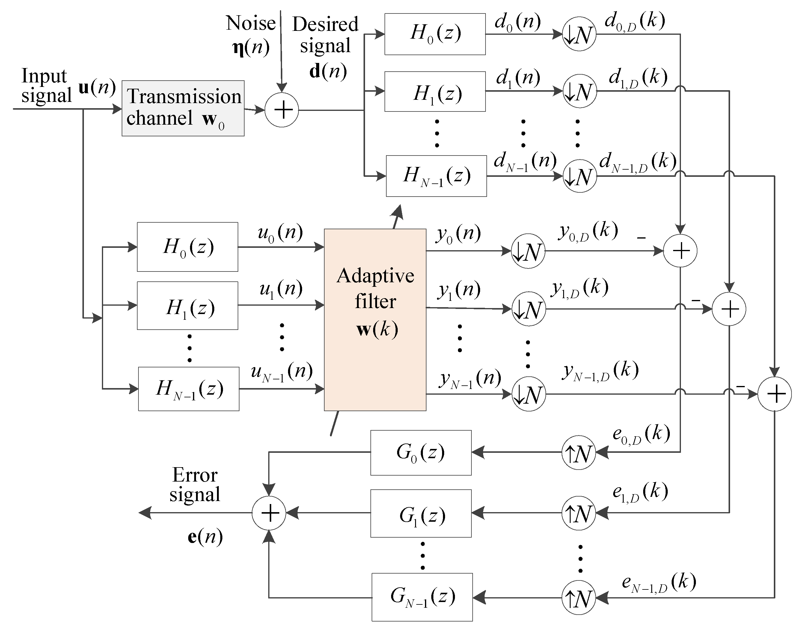
where ${\mathbf{w}}_0$ is the unknown weight vector, which should be estimated, and the length of ${\mathbf{w}}_0$ is M. $\mathbf{u}\left(n\right)=\left[u\right(n),u(n-1),\dots ,u(n-M+1\left)\right]$ is the input signal; the environment noise $\eta \left(n\right)$ is the white Gaussian noise; and the variance of $\eta \left(n\right)$ is ${\sigma }_{\eta }^2$. The structure of the NSAF algorithm is shown in Figure 1.

Subsequently, $\mathbf{u}\left(n\right)$, $d\left(n\right)$, and $\eta \left(n\right)$ are divided into N sub-band signals by the filters $H_0\left(z\right),H_1\left(z\right),\dots ,H_{N-1}\left(z\right)$, respectively. ${\mathbf{u}}_i\left(n\right)$, $d_i\left(n\right)$, and ${\eta }_i\left(n\right)$ are the corresponding sub-band signals, $i=0,1,\dots ,N-1$. The sub-band signals $y_i\left(n\right)$ and $d_i\left(n\right)$ are critically decimated to generate the signals $y_{i,D}\left(k\right)$ and $d_{i,D}\left(k\right)$, respectively. $y_{i,D}\left(k\right)={\mathbf{u}}_i^T\left(k\right)\mathbf{w}\left(k\right)$ is the output of the ith sub-band filter. In each of the above equations, n indicates the sequence number of the original signal, and k indicates the sequence number of the decimated sequences. Therefore, the input signal, the desired output signal, and the output error can be represented as:

$$\mathbf{U}\left(k\right)=[{\mathbf{u}}_0\left(k\right),{\mathbf{u}}_1\left(k\right),\dots ,{\mathbf{u}}_{N-1}\left(k\right)]$$

(2)

$${\mathbf{d}}_D\left(k\right)=[d_{0,D}\left(k\right),d_{1,D}\left(k\right),...,d_{N-1,D}\left(k\right)]={\mathbf{U}}^T\left(k\right){\mathbf{w}}_0+\eta \left(k\right)$$

(3)

$${\mathbf{e}}_D\left(k\right)={\mathbf{d}}_D\left(k\right)-{\mathbf{U}}^T\left(k\right)\mathbf{w}\left(k\right)=[e_{0,D}\left(k\right),e_{1,D}\left(k\right),...,e_{N-1,D}\left(k\right)]$$

(4)

The original NSAF algorithm is proposed with the principle of minimal disturbance, and the Lagrangian multiplier method is used to determine the optimal solution. Thus, the update weight vector of the NSAF algorithm is obtained as follows:

$$\mathbf{w}(k+1)=\mathbf{w}\left(k\right)+\mu \sum _{i=0}^{N-1}\frac{e_{i,D}\left(k\right){\mathbf{u}}_i\left(k\right)}{\parallel {\mathbf{u}}_i{\left(k\right)\parallel }^2+\delta }$$

(5)

where $\mu$ is the step-size, $\parallel ·\parallel$ indicates the norm of a vector, and the term $\delta$ is the regularization parameter.

2.2. The $\alpha$-Stable Distribution Impulsive Noise

For SI cancellation in ISUDC, the environmental noise (wave noise, wind noise, biological activity, etc.) is a non-Gaussian distribution in the underwater acoustic channel. Its amplitude is much higher than its uniform value at some moments, and it has remarkable pulse characteristics. The impulsive noise with the $\alpha$-stable distribution is more consistent with the description of this noise model in the actual environment by related research [26], and its characteristic function can be expressed as:

$$f\left(t\right)=exp\{j\delta t-\gamma |t{|}^{\alpha }\left[1+j\beta \mathrm{sgn}\left(t\right)S(t,\alpha )\right]\}$$

(6)

with the notation:

$$S(t,\alpha )=\left\{\begin{array}{cc}tan\frac{\alpha \pi }{2},\hfill & \mathrm{when}\alpha \ne 1;\hfill \\ \frac{2}{\pi }log\left|t\right|,\hfill & \mathrm{when}\alpha =1.\hfill \end{array}\right.$$

(7)

Form Equation (6), we know that the characteristic function can be determined by $\left[\alpha ,\beta ,\gamma ,\delta \right]$. The four parameters reflect the different characteristics of the impulse noise; $\alpha \in (0,2]$ represents the characteristic factor; $\beta \in [-1,1]$ represents the symmetry parameter; $\gamma >0$ represents the dispersion parameter; and $\delta$ represents the location parameter. The impulse noise mentioned in the following research is generated by this impulse noise model.

3. Proposed Algorithm

3.1. Arctangent Cost Function

To improve the robustness of the original NSAF algorithm against the impulsive noise, the arctangent cost function is applied to the LMS algorithm [27], and the updated weight vector is adjusted. The relationship between $\mathbf{w}\left(k\right)$ and the arctangent cost function can be expressed as follows:

$$J\left(\mathbf{w}\left(k\right)\right)=E\left[\frac{arctan\left(\beta {\left(\frac{e_i\left(k\right)}{\parallel {\mathbf{u}}_i\left(k\right)\parallel }\right)}^2\right)}{2\beta }\right]$$

(8)

where $\beta (0<\beta \le 100)$ is the control parameter, and it reflects the cost function to the output error $e_i\left(k\right)$.

The arctangent cost function is simple to construct and only needs $e_i\left(k\right)$ and input signal ${\mathbf{u}}_i\left(k\right)$, and two variables can be obtained directly. Its calculation complexity is small, which is convenient for engineering implementation. The input signal is divided into several sub-bands by an adaptive filter, respectively, in the NSAF algorithm. According to Equation (8), we apply the arctangent cost function to the NSAF algorithm and can get:

$$J\left(\mathbf{w}\left(k\right)\right)=\sum _{i=0}^{N-1}E\left[\frac{arctan\left(\beta {\left(\frac{e_{i,D}\left(k\right)}{\parallel {\mathbf{u}}_i\left(k\right)\parallel }\right)}^2\right)}{2\beta }\right]$$

(9)

To reduce the iteration error along the direction of the iteration, Equation (9) can be transformed as the following equation by the negative stochastic gradient method.

$$\nabla J\left(\mathbf{w}\left(k\right)\right)=\sum _{i=0}^{N-1}E\left(\frac{{\mathbf{u}}_i\left(k\right)e_{i,D}\left(k\right)}{\parallel {\mathbf{u}}_i{\left(k\right)\parallel }^2+\frac{{\beta }^2{e}_{i,D}^4\left(k\right)}{\parallel {\mathbf{u}}_i{\left(k\right)\parallel }^2}}\right)$$

(10)

so the weight update formula is written as:

$$\mathbf{w}(k+1)=\mathbf{w}\left(k\right)+\mu \sum _{i=0}^{N-1}\frac{e_{i,D}\left(k\right){\mathbf{u}}_i\left(k\right)}{\parallel {\mathbf{u}}_i{\left(k\right)\parallel }^2+\frac{{\beta }^2{e}_{i,D}^4\left(k\right)}{\parallel {\mathbf{u}}_i{\left(k\right)\parallel }^2}}$$

(11)

According to Equation (11), the output error $e_{i,D}\left(k\right)$ is small when there is no impulsive noise, and ${\beta }^2{e}_{i,D}^4\left(k\right)/{\parallel {\mathbf{u}}_i\left(k\right)\parallel }^2$ tends to zero with the increasing of the iteration times. The signal is distorted, and the amplitude increases sharply when the impulsive noise appears. As a result, ${\beta }^2{e}_{i,D}^4\left(k\right)/{\parallel {\mathbf{u}}_i\left(k\right)\parallel }^2$ increases sharply, and the latter term of the weight update formula tends to zero, that is the descending direction tends to be unchanged. Therefore, the weight vector update error resulting from the impulsive noise can be effectively reduced.

Hence, the weight vector hardly changes, and it is approximately equal to the weight vector of the previous step when impulsive noise occurs. The weight vector update is close to the NSAF algorithm when there is no impulsive noise. Therefore, the improved NSAF algorithm is insensitive to the impulsive noise and has excellent impulsive noise resistance. This algorithm is an improved NSAF algorithm based on the arctangent cost function, so it is called Arc-NSAF.

3.2. Arc-IPNSAF Algorithm

The proportionate adaptation technique can be combined with the Arc-NSAF algorithm to adapt to the sparse SI channel. We introduce this technique into the Arc-NSAF algorithm, and $\mathbf{w}\left(k\right)$ is represented as:

$$\mathbf{w}(k+1)=\mathbf{w}\left(k\right)+\mu \sum _{i=0}^{N-1}\frac{e_{i,D}\left(k\right)\mathbf{Q}\left(k\right){\mathbf{u}}_i\left(k\right)}{{\mathbf{u}}_i^T\left(k\right)\mathbf{Q}\left(k\right){\mathbf{u}}_i\left(k\right)+\frac{{\beta }^2{e}_{i,D}^4\left(k\right)}{\parallel {\mathbf{u}}_i{\left(k\right)\parallel }^2}}$$

(12)

The gain matrix $\mathbf{Q}\left(k\right)=diag\{q_1\left(k\right),q_2\left(k\right),\dots ,q_M\left(k\right)\}$ is an $M\times M$ diagonal matrix, and its diagonal elements can be calculated as follows:

$$q_m\left(k\right)=\frac{1-\kappa }{2M}+\left(1+\kappa \frac{|w_m\left(k\right)|}{{2\parallel \mathbf{w}\left(k\right)\parallel }_1+\xi }\right)$$

(13)

with $\xi$ a small positive constant and the control parameter $\kappa \in [-1,1]$, and it is usually taken as −0.5 or zero.

3.3. Improved Arc-IPNSAF Algorithm

The underwater acoustic channel is a stochastic acoustic propagation channel with time, space, and frequency varying, and the sparsity of the channel varies with the environment. The degree of sparsity for a channel [28] can be quantified as follows:

$$\psi \left({\mathbf{w}}_0\right)=\frac{M}{M-1}\left(1-\frac{\parallel {\mathbf{w}}_0{\parallel }_1}{\sqrt{M}{\parallel {\mathbf{w}}_0\parallel }_2}\right)$$

(14)

Obviously, we can get $0\le \psi \left({\mathbf{w}}_0\right)\le 1$ by Equation (14). The sparser the channel is, the larger the value $\psi \left({\mathbf{w}}_0\right)$ is. Since ${\mathbf{w}}_0$ is unknown, $\mathbf{w}\left(k\right)$ is used to approximate substitution ${\mathbf{w}}_0$ at each iteration, and the sparsity estimates for each iteration are shown below:

$$\widehat{\psi }\left(\mathbf{w}\left(k\right)\right)=\frac{M}{M-\sqrt{M}}\left(1-\frac{{\parallel \mathbf{w}\left(k\right)\parallel }_1}{\sqrt{M}{\parallel \mathbf{w}\left(k\right)\parallel }_2}\right)$$

(15)

Apparently, $\widehat{\psi }\left(\mathbf{w}\left(k\right)\right)$ will gradually converge to $\psi \left({\mathbf{w}}_0\right)$ with the increasing of the iteration times. Therefore, the sparsity of the channel can be estimated and quantified in each iteration of the algorithm.

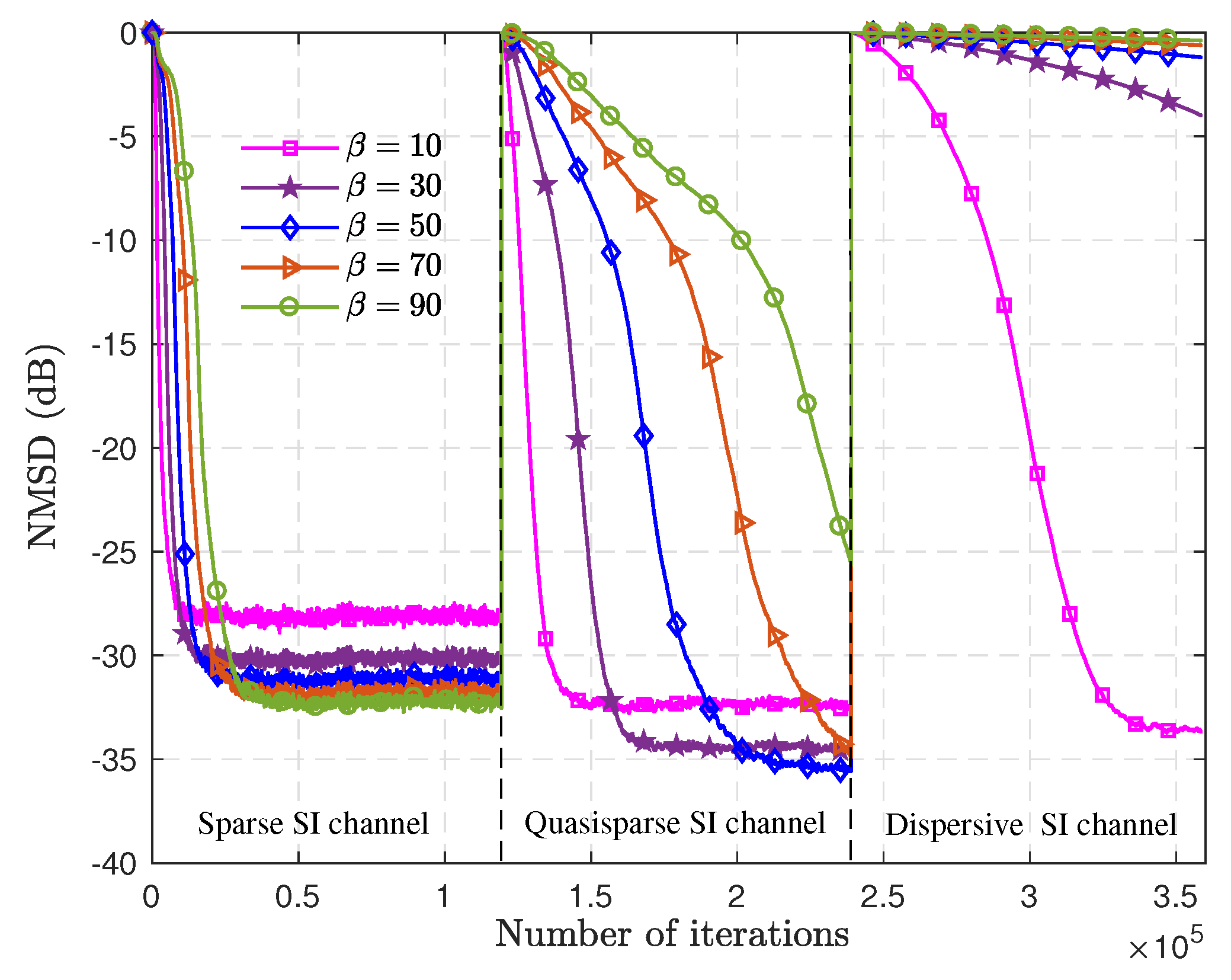
Analyzing Equation (12) again, the control parameter $\beta$ in Equation (12) has some effect on the performance of the algorithm. Some simulation results are used to illustrate the effect of the control parameter on the algorithm. The performance is evaluated by the normalized mean squared deviation (NMSD), which is:

$$NMSD=10log\left(\frac{\parallel \widehat{\mathbf{w}}{\left(k\right)\parallel }_2^2}{\parallel {\mathbf{w}}_0{\parallel }_2^2}\right)$$

(16)

We define $\widehat{\mathbf{w}}\left(k\right)={\mathbf{w}}_0-\mathbf{w}\left(k\right)$. NMSD reflects the closeness between the estimated weight vector $\widehat{\mathbf{w}}\left(k\right)$ and the real weight vector ${\mathbf{w}}_0$, and it can also be regarded as the steady-state error of the algorithm. Figure 2 shows the performance comparison in three different SI channels with different $\beta$.

Figure 2 shows the influence of $\beta$ on the convergence speed and steady-state error of the algorithm. Comparing the performance of the algorithm with different $\beta$ in the same SI channel, we can know that the steady-state error decreases with an increase of $\beta$, and the convergence speed decreases. The sparsity of the SI channel also affects the convergence speed and steady-state error of the algorithm. Comparing the performance of the algorithm with the same $\beta$ in different SI channels, the convergence speed decreases with the increase of the sparsity, while the steady-state error decreases. Therefore, we make a compromise on the convergence speed and steady-state error of the algorithm and improve the robustness of the algorithm to the SI channel with different sparsity. It is necessary to take a relatively large value of $\beta$ when the sparsity of the SI channel is large, so that the algorithm can obtain a smaller steady-state error. Similarly, $\beta$ should take a relatively small value to obtain a faster convergence speed when the sparsity of the SI channel is small. According to the relevant research on the influence of the sparsity of the SI channel on the performance of IPNLMS algorithm in [29,30], we construct the adaptive control parameter $\beta \left(k\right)$ with the sparsity measurement values $\widehat{\psi }\left(\mathbf{w}\left(k\right)\right)$ to approximate the curve of the relationship, which is expressed as:

$$\beta \left(k\right)=\left\{\begin{array}{cc}ϵ,\hfill & \mathrm{if}k<MN;\hfill \\ \gamma ·e^{\lambda (\widehat{\psi }\left(\mathbf{w}\left(k\right)\right)-1)},\hfill & \mathrm{others}.\hfill \end{array}\right.$$

(17)

where $ϵ$ is an initial value, which is a small positive constant. $\gamma$ determines the amplitude change, and $\lambda$ determines the rate of change; they are constants greater than one. When $\gamma =1$, the corresponding conversion function values $\beta \left(k\right)$ with different $\lambda$ are as shown in Figure 3.

As shown in Figure 3, the larger the value of $\lambda$, the faster the changer of $\beta \left(k\right)$ is, and the smaller the value of $\beta \left(k\right)$. Therefore, $\beta \left(k\right)$ should be larger for the sparse channel and smaller for the dispersive channel. Based on the relationship between sparseness and the optimal value of $\beta$, as well as the simulation analysis, $\gamma =80$ and $\lambda =8$ are used in the subsequent research. Then, we replace $\beta$ in Equation (12) with $\beta \left(k\right)$, and we can get the final weight vector update equation of Arc-IPNSAF based on sparsity control.

$$\mathbf{w}(k+1)=\mathbf{w}\left(k\right)+\mu \sum _{i=0}^{N-1}\frac{e_{i,D}\left(k\right)\mathbf{Q}\left(k\right){\mathbf{u}}_i\left(k\right)}{{\mathbf{u}}_i^T\left(k\right)\mathbf{Q}\left(k\right){\mathbf{u}}_i\left(k\right)+\frac{{\beta }^2\left(k\right)e_{i,D}^4\left(k\right)}{\parallel {\mathbf{u}}_i{\left(k\right)\parallel }^2}}$$

(18)

The proposed algorithm is an improved IPNSAF algorithm based on sparsity control and the arctangent cost function, so we call the above proposed algorithm Sc-Arc-IPNSAF. The proposed algorithm can be applied to the same signal types as the traditional NSAF algorithm. The main iterative process of the algorithm is shown is shown as Algorithm 1.

Algorithm 1: Proposed the Sc-Arc-IPNSAF algorithm

Initialization:  $\mathbf{w}\left(0\right)=\mathbf{0}$; Parameter:  $\lambda$, $\gamma$ and $\xi$ are predefined;   1: Update:   2:    For each iteration k   3:       1. Calcuate the sparsity $\widehat{\psi }\left(\mathbf{w}\left(k\right)\right)$ of the SI channel   4:          $\widehat{\psi }\left(\mathbf{w}\left(k\right)\right)=\frac{M}{M-\sqrt{M}}\left(1-\frac{{\parallel \mathbf{w}\left(k\right)\parallel }_1}{\sqrt{M}{\parallel \mathbf{w}\left(k\right)\parallel }_2}\right)$   5:       2. The adaptive control parameters $\beta \left(k\right)$   6:          $\beta \left(k\right)=\left\{\begin{array}{c}ϵ,\mathrm{if}k<MN;\hfill \\ \gamma ·e^{\lambda (\widehat{\psi }\left(\mathbf{w}\left(k\right)\right)-1)},\mathrm{others}.\end{array}\right.$   7:     8:       3. Obtain the gain proportional matrix $\mathbf{Q}\left(k\right)$   9:          $q_m\left(k\right)=\frac{1-\kappa }{2M}+(1+\kappa \frac{|w_m\left(k\right)|}{{2\parallel \mathbf{w}\left(k\right)\parallel }_1+\xi })$ 10:       4. Weight vector update 11:          $\mathbf{w}(k+1)=\mathbf{w}\left(k\right)+\mu {\sum }_{i=0}^{N-1}\frac{e_{i,D}\left(k\right)\mathbf{Q}\left(k\right){\mathbf{u}}_i\left(k\right)}{{\mathbf{u}}_i^T\left(k\right)\mathbf{Q}\left(k\right){\mathbf{u}}_i\left(k\right)+\frac{{\beta }^2\left(k\right)e_{i,D}^4\left(k\right)}{\parallel {\mathbf{u}}_i{\left(k\right)\parallel }^2}}$ 12:    End

4. Algorithm Performance Analysis

4.1. Convergence Performance

The convergence performance of the Sc-Arc-IPNSAF algorithm is analyzed. To calculate the analysis, substitute $\widehat{\mathbf{w}}\left(k\right)={\mathbf{w}}_0-\mathbf{w}\left(k\right)$ into Equation (18); we can get:

$$\widehat{\mathbf{w}}(k+1)=\widehat{\mathbf{w}}\left(k\right)-\mu \mathbf{Q}\left(k\right)\mathbf{U}\left(k\right){\Lambda }^{-1}\left(k\right){\mathbf{e}}_D\left(k\right)$$

(19)

with $\Lambda \left(k\right)={\mathbf{U}}^T\left(k\right)\mathbf{Q}\left(k\right)\mathbf{U}\left(k\right)+\phi \mathbf{I}$, and the notation $\mathbf{I}$ expresses an $M\times M$ identity matrix, and $\phi ={\beta }^2\left(k\right)e_{i,D}^4\left(k\right)/{\parallel {\mathbf{u}}_i\left(k\right)\parallel }^2$.

Define ${\mathbf{e}}_a\left(k\right)={\mathbf{U}}^T\left(k\right)\widehat{\mathbf{w}}\left(k\right)$ and ${\mathbf{e}}_b\left(k\right)={\mathbf{U}}^T\left(k\right)\widehat{\mathbf{w}}(k+1)$; their physical meanings are the a-priori and b-posteriori sub-band error vectors, respectively. It can be noted that ${\mathbf{e}}_a\left(k\right)$ and ${\mathbf{e}}_b\left(k\right)$ do not contain the error of the system noise, so we can get:

$${\mathbf{e}}_b\left(k\right)={\mathbf{e}}_a\left(k\right)-\mu {\mathbf{U}}^T\left(k\right)\mathbf{Q}\left(k\right)\mathbf{U}\left(k\right){\Lambda }^{-1}{\mathbf{e}}_D\left(k\right)$$

(20)

Assume that $\mathbf{U}\left(k\right)$ is column full rank, so ${\mathbf{U}}^T\left(k\right)\mathbf{Q}\left(k\right)\mathbf{U}\left(k\right)$ is invertible. Substitute Equation (20) into Equation (19), and define ${\parallel \mathbf{U}\left(k\right)\parallel }_{{\mathbf{Q}}^{-1}\left(k\right)}{\parallel }^2={\mathbf{U}}^T\left(k\right){\mathbf{Q}}^{-1}\left(k\right)\mathbf{U}\left(k\right)$ as the squared weighted Euclidean norm of $\mathbf{U}\left(k\right)$. Then, taking the expectation on both sides and supposing $k\to +\infty$, we have:

$$\begin{array}{cc}\hfill & \underset{k\to +\infty }{lim}\parallel \widehat{\mathbf{w}}{(k+1)\parallel }_{{\mathbf{Q}}^{-1}\left(k\right)}^2-\underset{k\to +\infty }{lim}{\parallel \widehat{\mathbf{w}}\left(k\right)\parallel }_{{\mathbf{Q}}^{-1}\left(k\right)}^2\hfill \\ \hfill =& \underset{k\to +\infty }{lim}E\left({\mathbf{e}}_b^T\left(k\right){\left({\mathbf{U}}^T\left(k\right)\mathbf{Q}\left(k\right)\mathbf{U}\left(k\right)\right)}^{-1}{\mathbf{e}}_b\left(k\right)\right)\hfill \\ \hfill & -\underset{k\to +\infty }{lim}E\left({\mathbf{e}}_a^T\left(k\right){\left({\mathbf{U}}^T\left(k\right)\mathbf{Q}\left(k\right)\mathbf{U}\left(k\right)\right)}^{-1}{\mathbf{e}}_a\left(k\right)\right)\hfill \end{array}$$

(21)

It is known that $\phi$ goes to zero as the number of iterations increases $k\to \infty$, so we can get ${lim}_{k\to +\infty }E\left({\mathbf{U}}^T\left(k\right)\mathbf{Q}\left(k\right)\mathbf{U}\left(k\right)\right)\approx {lim}_{k\to +\infty }E\left(\Lambda \left(k\right)\right)$. Substituting Equation (20) into Equation (21) results in:

$$\begin{array}{cc}\hfill & \underset{k\to +\infty }{lim}\parallel \widehat{\mathbf{w}}{(k+1)\parallel }_{{\mathbf{Q}}^{-1}\left(k\right)}^2-\underset{k\to +\infty }{lim}{\parallel \widehat{\mathbf{w}}\left(k\right)\parallel }_{{\mathbf{Q}}^{-1}\left(k\right)}^2\hfill \\ & \approx {\mu }^2\underset{k\to +\infty }{lim}E\left({\mathbf{e}}_D^T\left(k\right){\Lambda }^{-1}\left(k\right){\mathbf{e}}_D\left(k\right)\right)-2\mu \underset{k\to +\infty }{lim}E\left({\mathbf{e}}_a^T\left(k\right){\Lambda }^{-1}\left(k\right){\mathbf{e}}_D\left(k\right)\right)\hfill \end{array}$$

(22)

When the algorithm is convergent and stable, $\parallel \widehat{\mathbf{w}}{\left(k\right)\parallel }_{{\mathbf{Q}}^{-1}\left(k\right)}^2$ should decrease monotonically, and it tends to a stable value. Therefore, the left side of the Equation (22) tends to zero. Following this requirement, if the algorithm can converge to a stable state, $\mu$ has to be constrained as follows:

$$0<\mu <2\frac{{lim}_{k\to +\infty }E\left({\mathbf{e}}_a^T\left(k\right){\Lambda }^{-1}\left(k\right){\mathbf{e}}_D\left(k\right)\right)}{{lim}_{k\to +\infty }E\left({\mathbf{e}}_D^T\left(k\right){\Lambda }^{-1}\left(k\right){\mathbf{e}}_D\left(k\right)\right)}$$

(23)

In a noiseless situation, ${\mathbf{e}}_D\left(k\right)$ is approximately equal to ${\mathbf{e}}_a\left(k\right)$, and the maximum value for the right side of Equation (23) is two. Based on this fact, the step-size must satisfy $0<\mu <2$ when the algorithm can converge to a stable state.

Meanwhile, analyze Equation (22) again. The algorithm converges to a stable state when the number of iterations $k\to \infty$, and we can know that the left side of Equation (22) tends to zero. Let us assume that sub-band system noise ${\eta }_i\left(k\right)$ and input signal ${\mathbf{u}}_i\left(k\right)$ are statistically independent. Equation (22) is rewritten as:

$$(2-\mu )\sum _{i=0}^{N-1}\underset{k\to +\infty }{lim}E\left(\frac{e_{a,i}^2\left(k\right)}{\Lambda \left(k\right)}\right)=\mu \sum _{i=0}^{N-1}\underset{k\to +\infty }{lim}E\left(\frac{{\eta }_i^2\left(k\right)}{\Lambda \left(k\right)}\right)$$

(24)

Because of the inherent decorrelation property of the sub-band structure, each signal in the sub-bands is independent by critical decimation, so Equation (24) is approximated as:

$$(2-\mu )\underset{k\to +\infty }{lim}E\left(\frac{e_{a,i}^2\left(k\right)}{\Lambda \left(k\right)}\right)=\mu \underset{k\to +\infty }{lim}E\left(\frac{{\eta }_i^2\left(k\right)}{\Lambda \left(k\right)}\right).$$

(25)

When the algorithm is effective, the disturbance of $\Lambda \left(k\right)$ is small for a high-order adaptive filter in the process of iterative convergence, such that:

$$(2-\mu )\underset{k\to +\infty }{lim}\frac{E\left(e_{a,i}^2\left(k\right)\right)}{E\left(\Lambda \left(k\right)\right)}=\mu \underset{k\to +\infty }{lim}\frac{E\left({\eta }_i^2\left(k\right)\right)}{E\left(\Lambda \left(k\right)\right)}$$

(26)

Simplify Equation (26); it can be given as:

$$E\left(e_{a,i}^2(\infty )\right)\simeq \frac{\mu }{2-\mu }E\left({\eta }_i^2(\infty )\right).$$

(27)

Then, substituting Equation (27) into Equation (22) yields the excess mean squared error (EMSE) of the steady-state for the Sc-Arc-IPNSAF algorithm.

$$J_{EMSE}(\infty )=\frac{1}{N}\sum _{i=0}^{N-1}\underset{k\to +\infty }{lim}E\left(e_{i,D}^2\left(k\right)\right),$$

(28)

where ${\sigma }_{{\eta }_i}^2$ expresses the variance of ${\eta }_i$, and its physical meaning is the power of the sub-band system noise. Meanwhile, inserting Equation (27) into Equation (28) leads to the theoretical steady-state EMSE, expressed as:

$$EMSE(\infty )\simeq \frac{\mu }{2-\mu }\frac{1}{N}\sum _{i=0}^{N-1}{\sigma }_{{\eta }_i}^2.$$

(29)

According to [28], the steady-state MSE can be calculated based on Equation (29) as follows:

$$\begin{array}{cc}\hfill MSE(\infty )& \simeq EMSE(\infty )+\frac{1}{N}\sum _{i=0}^{N-1}{\sigma }_{{\eta }_i}^2\hfill \\ \hfill & \simeq \frac{2}{2-\mu }\frac{1}{N}{\sigma }_{{\eta }_i}^2\hfill \end{array}$$

(30)

The above expressions show that the steady-state EMSE and MSE depend on the system noise of each sub-band ${\sigma }_{{\eta }_i}^2$ and the number of sub-bands N, independent of $\mathbf{G}\left(k\right)$.

4.2. Computational Complexity

The computational complexity of the Sc-Arc-IPNSAF algorithm is analyzed and compared with other referenced algorithms in this section. The computation complexity of these algorithms is mainly represented by M, N, and the length of analysis filter L. For the Sc-Arc-IPNSAF algorithm, the sparsity estimation of the SI channel and the coefficient calculation of the arctangent cost function need additional $M/N+4$ multiplications and $3M/N$ addition for each sub-band in each iteration. Moreover, the calculation of ${\beta }^2\left(k\right)e_{i,D}^4\left(k\right)/{\parallel {\mathbf{u}}_i\left(k\right)\parallel }^2$ needs additional $M/N+6$ multiplication and $M/N$ addition.

Table 1. Computational complexity of updating $\mathbf{w}\left(k\right)$ for one iteration. MCC, maximum correntropy criterion; IPNLMS, improved proportionate normalized least mean squares; Sc, sparsity control.

Algorithm	Multiplication	Addition
MCC	2M + 6	2M
Arc-NLMS	4M + 8	4M − 1
Arc-IPNLMS	6M + 9	6M − 2
NSAF	3M + 3$NL$ + 1	3M + 3$NL$ − 3N
IPNSAF	5M + 3$NL$ + 1	5M + 3$NL$ + 2$M/N$ − 3N
Arc-NSAF	4M + 3$NL$ + 6N + 1	4M + 3$NL$ − 3N
Arc-IPNSAF	6M + 3$NL$ + 6N + 1	6M + 3$NL$ + 2$M/N$ − 3N
Sc-Arc-IPNSAF	7M + 3$NL$ + 10N + 1	8M + 3$NL$ + 2$M/N$

shows that the Sc-Arc-IPNSAF algorithm has the highest computational complexity, and the MCC algorithm is the lowest because the sparsity of the SI channel is estimated. The coefficient of the cost function is adaptively adjusted to satisfy the SI channel with different sparsity. The Sc-Arc-IPNSAF algorithm only increases the 2M + 10N multiplication and 3M−3N addition compared with the IPNSAF algorithm. As a comparison, the additional computational complexity of Sc-Arc-IPNSAF is still in the same order of magnitude as other referenced algorithms, and it can be acceptable and easy to implement in engineering hardware.

The memory requirements of each algorithm can be calculated according to the storage of the filter structure and the data storage required in the iterative process. The memory requirement of the traditional NSAF algorithm is M(N + 1) + N(3L + 4) + 2 [14]. Because the IPNSAF algorithm needs to calculate the gain matrix, it requires an additional $NM+2$ memory to store the gain matrix and the parameters compared with the NSAF algorithm. The Sc-Arc-IPNSAF algorithm needs to store the sparsity of the SI channel $\widehat{\psi }\left(\mathbf{w}\left(k\right)\right)$, the control parameters $\beta \left(k\right)$, and $\phi$. Therefore, it needs an additional 3N memory compared with the IPNSAF algorithm. Therefore, we can get the memory requirements of the algorithms, as shown in

Table 2. Memory requirements for each algorithm.

Algorithm	Memory
MCC	2M + 5
Arc-NLMS	2M + 6
Arc-IPNLMS	3M + 8
NSAF	M(N + 1) + N(3L + 4) + 2
IPNSAF	M(2N + 1) + N(3L + 4) + 4
Arc-NSAF	M(N + 1) + N(3L + 5) + 2
Arc-IPNSAF	M(2N + 1) + N(3L + 5) + 4
Sc-Arc-IPNSAF	M(2N + 1) + N(3L + 7) + 4

.

5. Simulation

The proposed algorithm is evaluated in different system identification scenarios. Considering the application of the SI channel with variable sparsity, three different SI channels with 512 coefficients are used in the following simulation experiments. The impulse response of three SI channels is shown in Figure 4. For all algorithms, the initial weight vector $\mathbf{w}\left(0\right)=\mathbf{0}$, the initial step-size ${\mu }_0=0.1$, and the relevant parameters of the NSAF class algorithms are set to $L=64$, $N=8$. Therefore, we can get that each iteration of the proposed algorithm requires 5201 multiplications and 5760 additions according to Table 1. The two-order autoregressive (AR(2)) signal is used as an input signal to validate the proposed algorithm. Furthermore, SI is the communication signal leaked from the transmitter in ISUDC, so the BPSK modulated signal as the common communication signal is also used as another input signal to validate the feasibility of SI cancellation in ISUDC. For the BPSK modulated signal, the frequency bandwidth is 4–8 kHz, the sampling frequency is $f_s$ = 48 kHz, and the carrier frequency is $f_c$ = 6 kHz. The performance of the algorithms is compared with the same number of iterations. In the simulation experiment, when the input signal is the AR(2) signal, the number of iterations is set to 119,500, and the number of iterations is set to 180,000 when the input signal is the BPSK signal. The purpose of SI cancellation is to improve the performance of target parameter estimation, and the direction of arrival (DOA) is an important estimation parameter of ISUDC, so we compare the DOA estimation performance for the output signal after the SI cancellation. We consider two kinds of noise models in the following simulation experiments, the white Gaussian noise and the $\alpha$-stable distribution impulsive noise.

5.1. White Gaussian Noise

When the environment noise is the white Gaussian noise and the SNR is 40 dB, different algorithms are compared in three SI channels with different sparsity. Then, independent Monte Carlo simulation experiments are conducted 1000 times to obtain these results as Figure 5 and Figure 6.

The above simulation results show the NMSD results of different algorithms when the input signal has white Gaussian noise. As can be seen, the IPNSAF and the Sc-Arc-IPNSAF algorithms have similar performance, and even better than the others when the BPSK signal is input. Meanwhile, the IPNSAF and the Sc-Arc-IPNSAF algorithms have faster convergence speed than the others with the AR(2) signal input. In comparison, the Arc-IPNSAF algorithm without sparsity control has a slower convergence speed as the sparsity of the SI channel increases, but it is superior to the MCC algorithm. Therefore, the Sc-Arc-IPNSAF algorithm has excellent performance under the white Gaussian noise environment, and it is robust to the SI channel with different sparsity.

5.2. Impulsive Noise

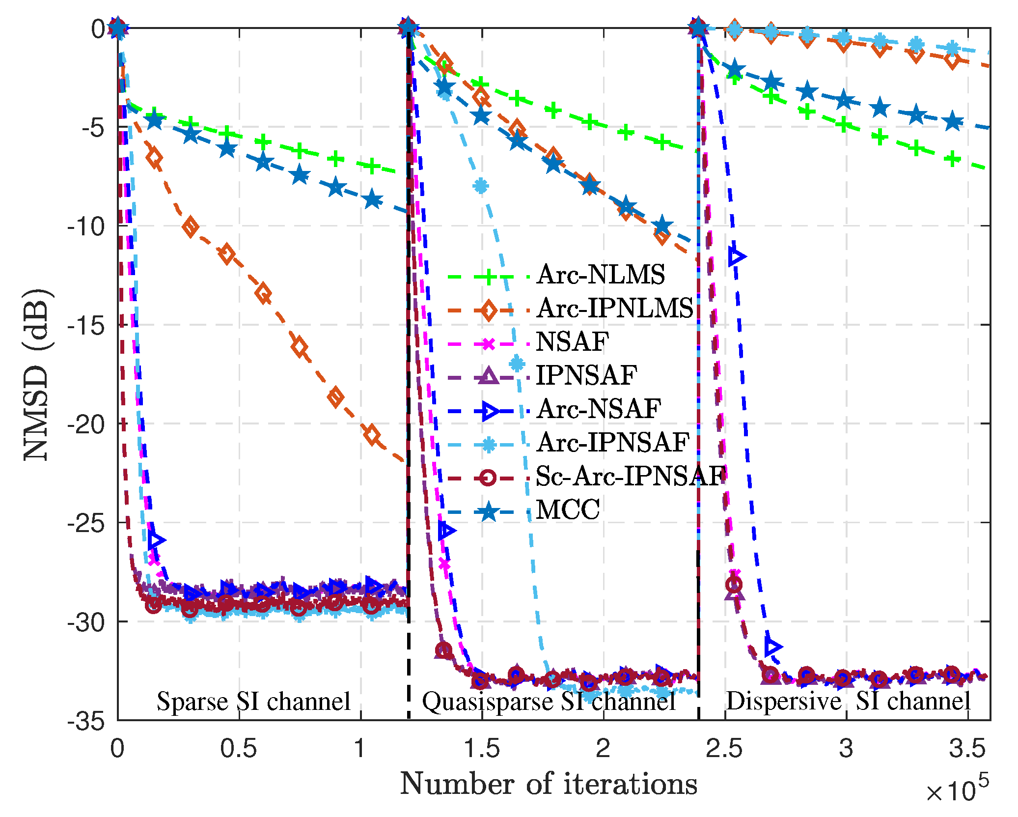
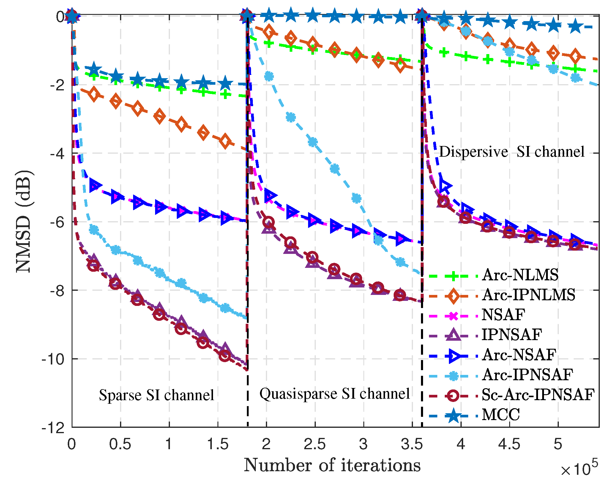
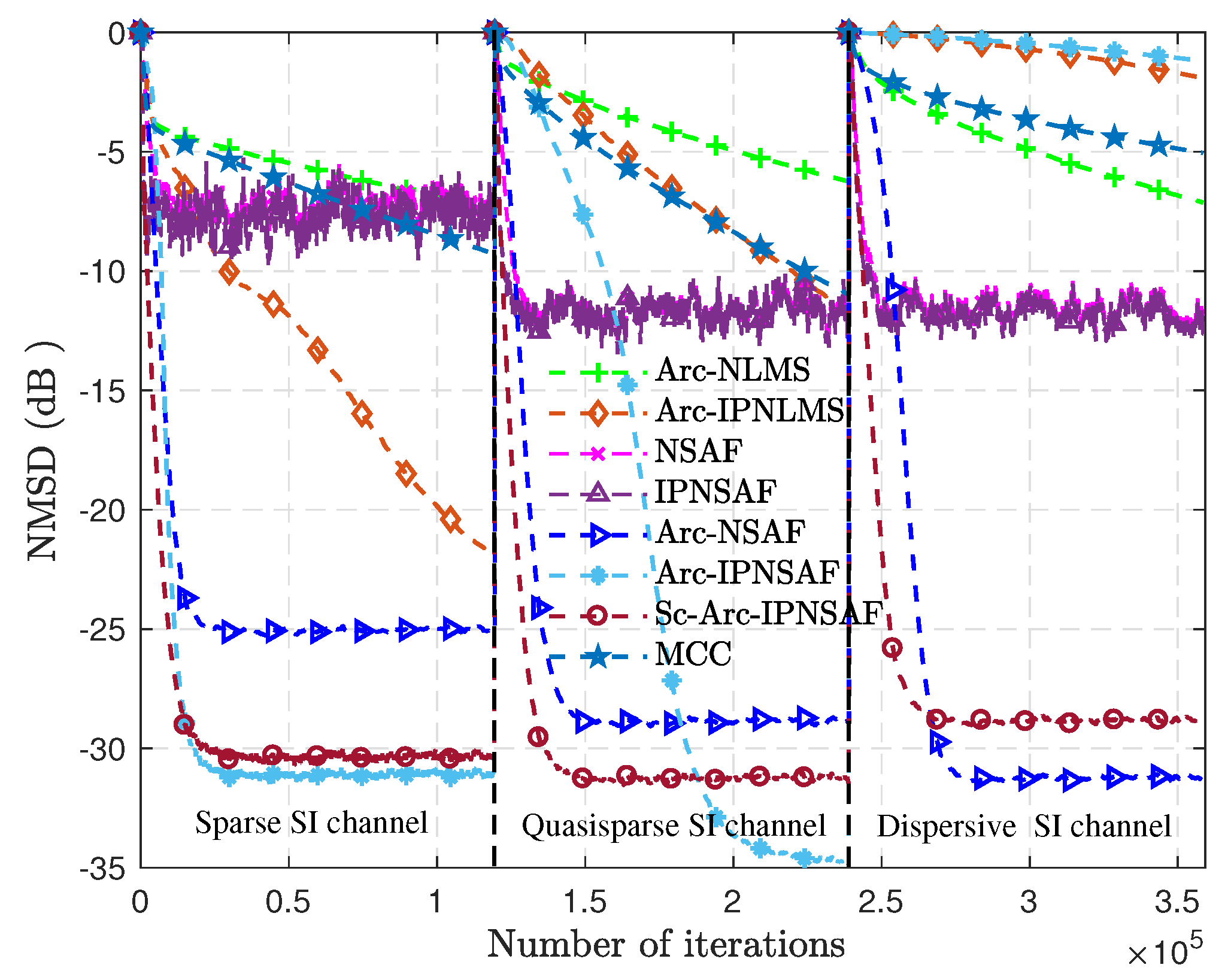
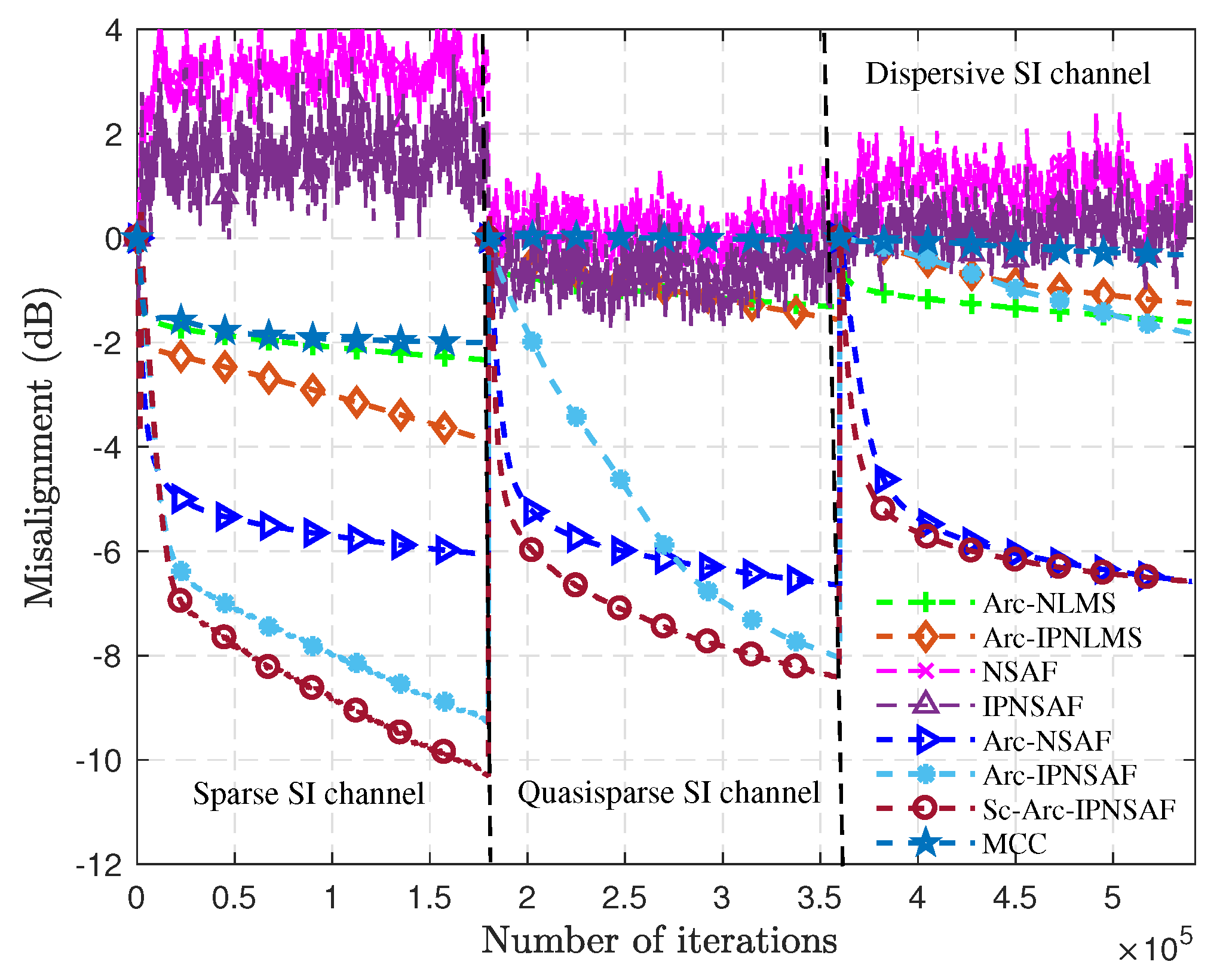
When the environment noise is the $\alpha$-stable distribution impulsive noise, which is produced by Equation (6), $\left(\alpha ,\beta ,\gamma ,\delta \right)=\left(1.2,0,0.2,0\right)$. The power of impulsive noise is set as ${\sigma }_I^2=1000{\sigma }_y^2$, where ${\sigma }_y^2$ is the power of the filter output for each sub-band $y_i\left(k\right)$. Then, different algorithms are compared in sparse, quasisparse, and dispersive SI channels with different input signals. Figure 7 and Figure 8 are obtained by Monte Carlo simulation experiments conducted 1000 times.

As can be seen from Figure 7 and Figure 8, the Sc-Arc-IPNSAF algorithm has a faster convergence speed for different SI channels, and its NMSD is smaller when the BPSK signal is input. Still, the NSAF and the IPNSAF algorithms are ineffective and cannot eliminate SI normally. In addition, the Sc-Arc-IPNSAF algorithm has stable performance for different SI channels and is better than the MCC, Arc-NLMS, Arc-IPNLMS, NSAF, and IPNSAF algorithms when the AR(2) signal is input. Unfortunately, it is unacceptable that the convergence speed of the Arc-IPNSAF algorithm drops sharply under the dispersive SI channel. Therefore, the Sc-Arc-IPNSAF algorithm improves the robustness for different sparsity SI channels with sparsity control.

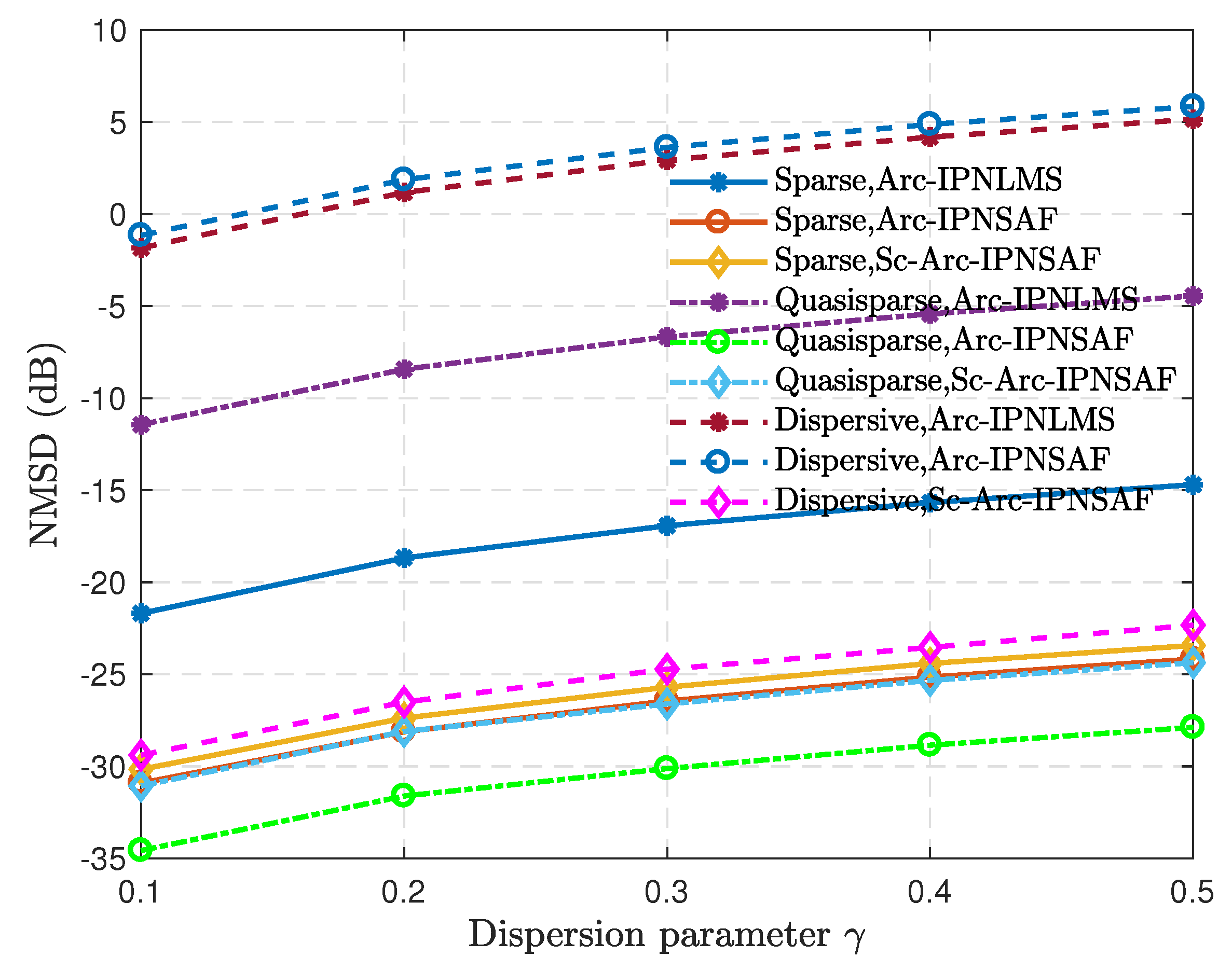
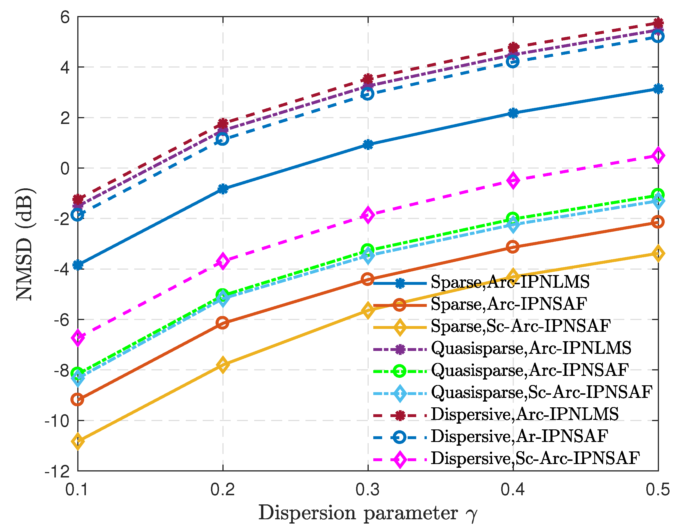
To compare the robustness of the algorithm with different impulsive noises, $\gamma$ in the $\alpha$-state distribution function is set to different values ($\gamma$ = 0.1:0.1:0.5). Monte Carlo simulation experiments conducted 1000 times obtain the results in Figure 9 and Figure 10.

From the simulation results, the performance of these algorithms deteriorates with the increase of $\gamma$, and these algorithms without sparsity control fail as $\gamma$ increases to some degree. Moreover, the Sc-Arc-IPNSAF algorithm has a low steady-state NMSD for different SI channels when the BPSK signal is the input signal. The Arc-type algorithms without sparsity control have a significant difference in performance under the different sparsity SI channels. The Sc-Arc-IPNSAF algorithm has stable performance for different SI channels, and the Arc-IPNSAF has similar performance in the sparse and quasisparse SI channels. Besides, the Sc-Arc-IPNSAF algorithm also has the best performance when the SI channel is dispersive, but the Arc-IPNSAF algorithm has the worst performance.

In other words, the proposed Sc-Arc-IPNSAF algorithm has good robustness and performance for different input signals and SI channels. Especially for the BPSK communication signal, the proposed Sc-Arc-IPNSAF algorithm has the best performance compared to the other referenced algorithms.

5.3. DOA Estimation Performance after SI Cancellation

In this simulation, consider the application of SI cancellation in ISUDC. For the integrated system, the transmitter transmits the BPSK communication modulation signal, and the signal parameter is as mentioned above. The receiver is an eight element uniform line array (ULA), and the separation between the elements is a half wavelength. The underwater speed of sound is c = 1490 m/s, and we assume that the SI direction is 0. In this section, the multiple signal classification (MUSIC) algorithm is used to estimate the DOA.

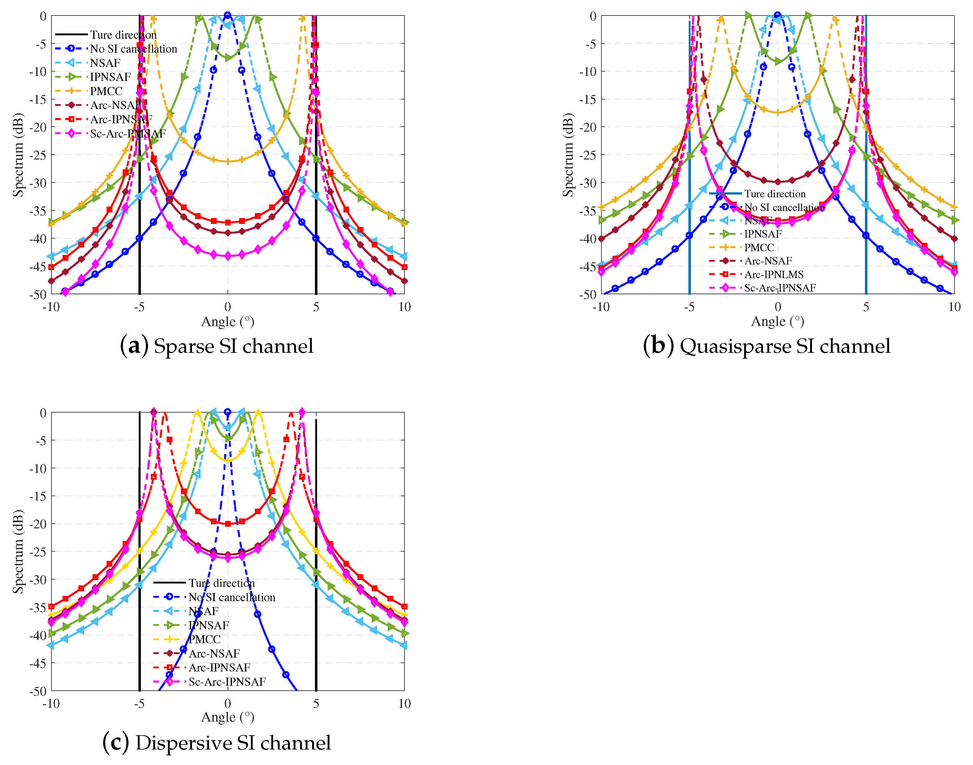
Compare the beamforming spectrum of the received signal after SI cancellation by different algorithms. In the simulation, the directions of two targets are at $-5$ and 5, and impulse noise is added to the target echo. The power of the target echo to the power of the SI ratio is called SIR, and the SIR is −16 dB in the subsequent simulation. The spatial spectra of the received signal after SI cancellation are as follow.

Figure 11 shows the spatial spectra of the received signal processed by different SI cancellation algorithms under three different SI channels. We know that the target cannot be estimated correctly without SI cancellation processing because the SI masks the target. While the two targets can be estimated after some adaptive filtering processing, the DOA estimation value of the received signal processed by the proposed algorithm is closest to the real value, which indicates that the estimation accuracy is the highest. The proposed algorithm has the optimal performance for different SI channels. Therefore, the Sc-Arc-IPNSAF algorithm has a good effect on the SI cancellation of ISUDC.

6. Conclusions

An improved IPNSAF algorithm is proposed for the SI channel with varying sparsity in impulsive noise, and it is called the Sc-Arc-IPNSAF algorithm. The proposed Sc-Arc-IPNSAF algorithm has a similar performance to the original NSAF algorithm when there is no impulsive noise. To suppress the error caused by the impulsive noise, the arctangent cost function is introduced so that the algorithm can resist impulse noise interference. Meanwhile, for the SI channel with varying sparsity, the sparsity of the SI channel is estimated and used to control the weight vector further. Comparing with some referenced algorithms, the simulation results confirm that the Sc-Arc-IPNSAF algorithm has a fast convergence speed, low NMSD, and good robustness against impulsive noise and a variable SI channel. From the results of DOA estimation, the SI cancellation improves the accuracy of DOA estimation, and the proposed algorithm has better performance of SI cancellation in ISUDC.

References

- Lu, J.; Zhang, Q.; Shi, W.; Zhang, L. High accuracy phase-matching delay estimation method based on phase correction. Iet Electron. Lett. 2020, 56, 456–459. [Google Scholar] [CrossRef]
- Qiao, G.; Gan, S.; Liu, S.; Song, Q. Self-Interference channel estimation algorithm based on Maximum-Likelihood estimator in In-Band Full-Duplex Underwater Acoustic communication system. IEEE Access 2018, 6, 62324–62334. [Google Scholar] [CrossRef]
- Qiao, G.; Gan, S.; Liu, S.; Ma, L.; Sun, Z. Digital self-interference cancellation for asynchronous in-band full-duplex underwater acoustic communication. Sensors 2018, 18, 1700–1716. [Google Scholar] [CrossRef] [PubMed] [Green Version]
- Li, C.; Zhao, H.; Wu, F.; Tang, Y. Digital Self-Interference Cancellation with Variable Fractional Delay FIR Filter for Full-Duplex Radios. IEEE Commun. Lett. 2018, 22, 1082–1085. [Google Scholar] [CrossRef]
- Ahmed, E.; Eltawil, A.M. All-Digital Self-Interference Cancellation Technique for Full-Duplex Systems. IEEE Trans. Wirel. Commun. 2015, 14, 3519–3532. [Google Scholar] [CrossRef] [Green Version]
- Shen, L.; Henson, B.; Zakharov, Y.; Mitchell, P. Digital self-interference cancellation for full-duplex underwater acoustic systems. IEEE Trans. Circ. Syst. 2020, 67, 192–196. [Google Scholar] [CrossRef] [Green Version]
- Shen, L.; Henson, B.; Zakharov, Y.; Mitchell, P. Two-Stage Self-Interference Cancellation for Full-Duplex Underwater Acoustic Systems. In Proceedings of the OCEANS 2019-Marseille, Marseille, France, 17–20 June 2019; pp. 1–6. [Google Scholar]
- Zha, D.; Qiu, T. Underwater sources location in non-Gaussian impulsive noise environments. Digit. Signal Process. 2006, 16, 149–163. [Google Scholar] [CrossRef]
- Mula, S.; Gogineni, V.C.; Dhar, A.S. Robust Proportionate Adaptive Filter Architectures Under Impulsive Noise. IEEE Trans. Very Large Scale Integr. (Vlsi) Syst. 2019, 27, 1223–1227. [Google Scholar] [CrossRef]
- Liu, W.; Pokharel, P.P.; Principe, J.C. Correntropy: Properties and Applications in Non-Gaussian Signal Processing. IEEE Trans. Signal Process. 2007, 55, 5286–5298. [Google Scholar] [CrossRef]
- He, R.; Hu, B.G.; Zheng, W.S.; Kong, X.W. Robust Principal Component Analysis Based on Maximum Correntropy Criterion. IEEE Trans. Image Process. 2011, 20, 1485–1494. [Google Scholar]
- Xiong, K.; Wang, S.; Chen, B. Robust normalized least mean absolute third algorithms. IEEE Access 2019, 7, 10318–10330. [Google Scholar] [CrossRef]
- Fu, Z.; Lin, Y. Robust Proportionate Adaptive Filtering Algorithms Against Impulsive Interference. In Proceedings of the International Conference on Computer, Mechatronics and Electronic Engineering 2017, Xiamen, China, 24–25 December 2017; pp. 258–264. [Google Scholar]
- Kuo, S.M.; Gan, W.S.; Lee, K.A. Subband Adaptive Filtering: Theory and Implementation; Wiley: Hoboken, NJ, USA, 2009. [Google Scholar]
- Lee, K.A.; Gan, W.S. Improving Convergence of the NLMS Algorithm Using Constrained Subband Updates. IEEE Signal Process. Lett. 2004, 11, 736–739. [Google Scholar] [CrossRef]
- Yu, Y.; Zhao, H.; He, Z.; Chen, B. A robust band-dependent variable step size NSAF algorithm against impulsive noises. Signal Process. 2016, 119, 203–208. [Google Scholar] [CrossRef]
- Diniz, P.S.R. Adaptive Filtering: Algorithms and Practical Implementation; Springer: Boston, MA, USA, 2002. [Google Scholar]
- Sayed, A.H. Fundamentals of Adaptive Filtering; Wiley: Hoboken, NJ, USA, 2003. [Google Scholar]
- Kadkhodazadeh, A.S. A family of proportionate normalized sub-band adaptive filter algorithms. J. Frankl. Inst. 2011, 348, 212–238. [Google Scholar]
- Li, Y.; Wang, Y.; Albu, F.; Jiang, J. A general zero attraction proportionate normalized maximum correntropy criterion algorithm for sparse system identification. Symmetry 2017, 9, 229. [Google Scholar] [CrossRef] [Green Version]
- Pelekanakis, K.; Chitre, M. Adaptive Sparse Channel Estimation under Symmetric alpha-Stable Noise. IEEE Trans. Wirel. Commun. 2014, 13, 3183–3195. [Google Scholar] [CrossRef]
- Pelekanakis, K.; Liu, H.; Chitre, M. An Algorithm for Sparse Underwater Acoustic Channel Identification under Symmetric alpha-Stable Noise. In Proceedings of the OCEANS 2011 IEEE-Spain, Santander, Spain, 6–9 June 2011. [Google Scholar]
- Ma, W.; Zheng, D.; Zhang, Z.; Duan, J.; Chen, B. Robust proportionate adaptive filter based on maximum correntropy criterion for sparse system identification in impulsive noise environments. Signal Image Video Process. 2018, 12, 117–124. [Google Scholar] [CrossRef]
- Gogineni, V.C.; Mula, S. Improved proportionate-type sparse adaptive filtering under maximum correntropy criterion in impulsive noise environments. Digit. Signal Process. 2018, 79, 190–198. [Google Scholar] [CrossRef]
- Kochanska, I. Assessment of Wide-Sense Stationarity of an Underwater Acoustic Channel Based on a Pseudo-Random Binary Sequence Probe Signal. Appl. Sci. 2020, 10, 1221. [Google Scholar] [CrossRef] [Green Version]
- Peng, S.; Chen, B.; Sun, L. Constrained maximum correntropy adaptive filtering. Signal Process. 2017, 140, 116–126. [Google Scholar] [CrossRef] [Green Version]
- Zeng, J.; Lin, Y.; Shi, L. A Normalized Least Mean Square Algorithm Based on the Arctangent Cost Function Robust Against Impulsive Interference. Circ. Syst. Signal Process. 2016, 35, 3040–3047. [Google Scholar] [CrossRef]
- Yu, Y.; Zhao, H. Proportionate NSAF algorithms with sparseness-measured for acoustic echo cancellation. Aeu-Int. J. Electron. Commun. 2017, 75, 53–62. [Google Scholar] [CrossRef] [Green Version]
- Liu, L.; Fukumoto, M.; Zhang, S. A variable parameter improved proportionate normalized LMS algorithm. IEEE Asia Pac. Conf. Circ. Syst. 2008, 201–204. [Google Scholar]
- Hirano, G.; Shimamura, T. A modified IPNLMS algorithm using system sparseness. In Proceedings of the 2012 International Symposium on Intelligent Signal Processing and Communications Systems, Taipei, Taiwan, 4–7 November 2012; pp. 876–879. [Google Scholar]
Figure 1.
The structure of normalized sub-band adaptive filtering (NSAF).
Figure 2.
Normalized mean squared deviation (NMSD) curves of Arc-improved proportionate NSAF (IPNSAF) with different under different self-interference (SI) channel environments.
Figure 3.
The adaptive control parameter varies with sparsity value when .
Figure 4.
The impulse response of three SI channels with different sparsity .
Figure 5.
NMSD of different algorithms in sparse, quasisparse, and dispersive SI channels, and the input signal is the AR(2) signal.
Figure 6.
NMSD of different algorithms in sparse, quasisparse, and dispersive SI channels, and the input signal is the BPSK signal.
Figure 7.
Figure 8.
Figure 9.
Steady-state NMSD with different for the AR(2) signal.
Figure 10.
Steady-state NMSD with different for the BPSK signal.
Figure 11.
The spatial spectra.