Constant Envelope Multiplexing of Multi-Carrier DSSS Signals Considering Sub-Carrier Frequency Constraint

Abstract

With the development of global navigation satellite systems (GNSS), multiple signals modulated on different sub-carriers are needed to provide various services and to ensure compatibility with previous signals. As an effective method to provide diversified signals without introducing the nonlinear distortion of High Power Amplifier (HPA), the multi-carrier constant envelope multiplexing is widely used in satellite navigation systems. However, the previous method does not consider the influence of sub-carrier frequency constraint on the multiplexing signal, which may lead to signal power leakage. By determining the signal states probability according to the sub-carrier frequency constraint and solving the orthogonal bases according to the homogeneous equations, this article proposed multi-carrier constant envelope multiplexing methods based on probability and homogeneous equations. The analysis results show that the methods can multiplex multi-carrier signals without power leakage, thereby reducing the impact on signal ranging performance. Meanwhile, the methods could reduce the computation complexity. In the case of three different carriers multiplexing, the number of optimization equations is reduced by nearly 66%.

1. Introduction

With the development of the global navigation satellite systems (GNSS), there is a great demand for providing diversified services and ensuring that the services are compatible with previous signals [1,2,3,4]. However, the limitation of power on satellite requests the signal to have a constant envelope. The most important reason is that the high power amplifier (HPA) has to operate in its full-saturation for maximum efficiency, ensuring that most of the energy is converted into signal power and transmitted to the earth. When the high power amplifier is working in the saturation region, the non-constant envelope signal will introduce amplitude modulation-amplitude modulation (AM-AM) and amplitude modulation-phase modulation (AM-PM) distortion, resulting in ranging distortion and power loss [5]. Therefore, how to construct a constant envelope signal has become a research hotspot, especially in the GNSS field.

Early GNSS signals only had two binary direct spread spectrum sequences (DSSS) modulated on the same carrier. It is easy to construct a constant envelope signal by modulating one binary DSSS signal on the in-phase and the other on the quadrature-phase, such as the C/A code and P(Y) code in the legacy GPS. The modulation is called quaternary phase shift keying (QPSK) [6]. As the number of DSSS signals increases, constant envelope multiplexing is not so simple. Interplex [7] and coherent adaptive subcarrier modulation (CASM) [8] are used to construct a constant envelope signal when more than two signals are multiplexed, and these two methods are proved to be mathematically equivalent. Although Interplex and CASM are very useful for three binary DSSS signals, as the number of DSSS signals increases, the multiplexing efficiency will reduce rapidly. Spiker and Orr proposed majority voting to use for the constant envelope multiplexing [9], and the upper bound of its multiplexing efficiency is not good enough. Cangiani, Orr, etc., proposed Inter-Vote, which is mixed Interplex and majority voting [10]. Although it improves multiplexing efficiency, it is still unsatisfactory in the case of more than five signals to be multiplexed. P. A. Dafesh and C. R. Cahn proposed phase-optimized constant-envelope transmission (POCET) [11], which is a very effective method for multiplexing more than 3 binary DSSS signals. This method is a constant envelope multiplexing method with optimal multiplexing efficiency. K. Zhang, H. Zhou, etc., proposed the multi-level POCET [12], which extended the multiplexed signals from binary to multi-level. Nevertheless, the POCET cannot intuitively reveal the relationship between various signal components. X.M. Zhang, X. Zhang, etc., proposed an inter-modulation construction method, revealing how to use the signal and its inter-modulation components to construct a POCET signal [13].

In addition to multiplexed signals at the same frequency point, there is also a need to multiplex signals with a constant envelope at multiple adjacent frequency points. Because if the signals modulated using different channels, the low interval between the bands would generate high propagation delays inside the desired band potentially leading to signal distortion and propagation time instability [14]. The first multi-frequency constant envelope signal in GNSS is the AltBOC [15], which is used in the Galileo system to emit the near band signals. ZuPing Tang, etc., proposed TD-AltBOC multiplexing different signals in different time slot [16]. The compatibility of this method is not well, and the number of multiplexed signals is limited. Zheng Yao, J Zhang, etc., proposed ACE-BOC, which is used for different signals power ratio [17]. Rotating POCET method is proposed by P. A. Dafesh and C. R. Cahn used for different frequency point [18]. Based on the inter-modulation construction method, Yao Zheng and Guo Fu, etc., proposed a method of constructing constant envelope signals at different frequencies based on the orthogonal basis [19]. Ma Junjie and Yao Zheng proposed the sub-carrier vector to describe the sub-carrier space on above method [20]. This method can flexibly multiplex multi-frequency and multi-level signals with constant envelope. However, the influence of sub-carrier frequency constraint on the signal states probability is not considered, and the method of constructing the orthogonal basis of multi-frequency signals based on tensor product is computationally expensive.

On the basis of orthogonal base multi-carrier constant envelope multiplexing, this article proposed multi-carrier constant envelope multiplexing methods based on probability and homogeneous equations. On the one hand, this method analyzes the influence of sub-carrier frequency constraint on the multiplexing signal by introducing the signal states probability, and constructs the multiplexing signal without signal power leakage based on this. On the other hand, this method solves orthogonal bases by homogeneous equations, which effectively reduces the number of orthogonal bases and optimization equations. As an effective multi-carrier constant envelope multiplexing method, it can flexibly select different frequency parameters to achieve constant envelope multiplexing according to frequency resources and signal design requirements, thereby improving the diversity and compatibility of GNSS signals.

This article is organized as follows: Section 2 will depict the constant envelope multiplexing principles. Section 3 will describe the constant envelope multiplexing based on probability and homogeneous equations. Section 4 provides the application of the method proposed in Section 3. Section 5 provides the analysis of the multiplexing signals. Section 6 gives the paper’s conclusions.

2. Constant Envelope Multiplexing Principles

Consider the combination of N independent DSSS signal components located at several adjacent frequencies, a generalized mixed radio frequency (RF) signal can be expressed as [17]:

$$S_{RF}={\displaystyle \sum _{i=1}^N\mathrm{Re}\left\{\sqrt{P_i}{s}_i\left(t\right)e^{j\left(2\pi f_{i}t+{\varphi }_i\right)}\right\}},$$

(1)

where $P_i$, $f_i$ and ${\varphi }_i$ are the nominal power, carrier frequency, and initial phase of the ith component, respectively; $s_i\left(t\right)$ is the ith baseband code signal decided by the data and pseudo-random noise (PRN) code.

As the signal’s RF frequency to emit is $f$, its initial phase is ${\varphi }_0$ and power is $P$, then the multiplexing RF signal can be expressed as:

$$\begin{gathered} S_{RF}=\mathrm{Re}\left\{\sqrt{P}\left[{\displaystyle \sum _{i=1}^N\sqrt{\frac{P_i}{P}}{s}_i\left(t\right)e^{j\left(2\pi \left(f_i-f\right)t+\left({\varphi }_i-{\varphi }_0\right)\right)}{e}^{j\left(2\pi ft+{\varphi }_0\right)}}\right]\right\}\hspace{0.17em}\hspace{0.33em} \\ =\mathrm{Re}\left\{\sqrt{P}\left[{\displaystyle \sum _{i=1}^N{A}_i{e}^{j\left(2\pi \Delta f_{i}t+\Delta {\varphi }_i\right)}{s}_i\left(t\right)}\right]e^{j\left(2\pi ft+{\varphi }_0\right)}\right\}\hspace{0.33em}\hspace{0.17em} \\ =\mathrm{Re}\left\{\sqrt{P}{S}_{SUM}{e}^{j\left(2\pi ft+{\varphi }_0\right)}\right\}, \end{gathered}$$

(2)

where $A_i=\sqrt{P_i/P}$ is the relative amplitude; $\Delta f_i$ and $\Delta {\varphi }_i$ are the frequency difference and initial phase difference between the ith signal and the emitting RF signal respectively; $e^{j\left(2\pi \Delta f_{i}t+\Delta {\varphi }_i\right)}$ is the sub-carrier of the ith signal; $S_{SUM}$ is the complex envelope of the N sum signals.

From the discussion above, $S_{SUM}$ could be expressed as:

$$S_{SUM}={\displaystyle \sum _{i=1}^N{A}_i{e}^{j\Delta {\varphi }_i}{e}^{j2\pi \Delta f_{i}t}{s}_i}\left(t\right).$$

(3)

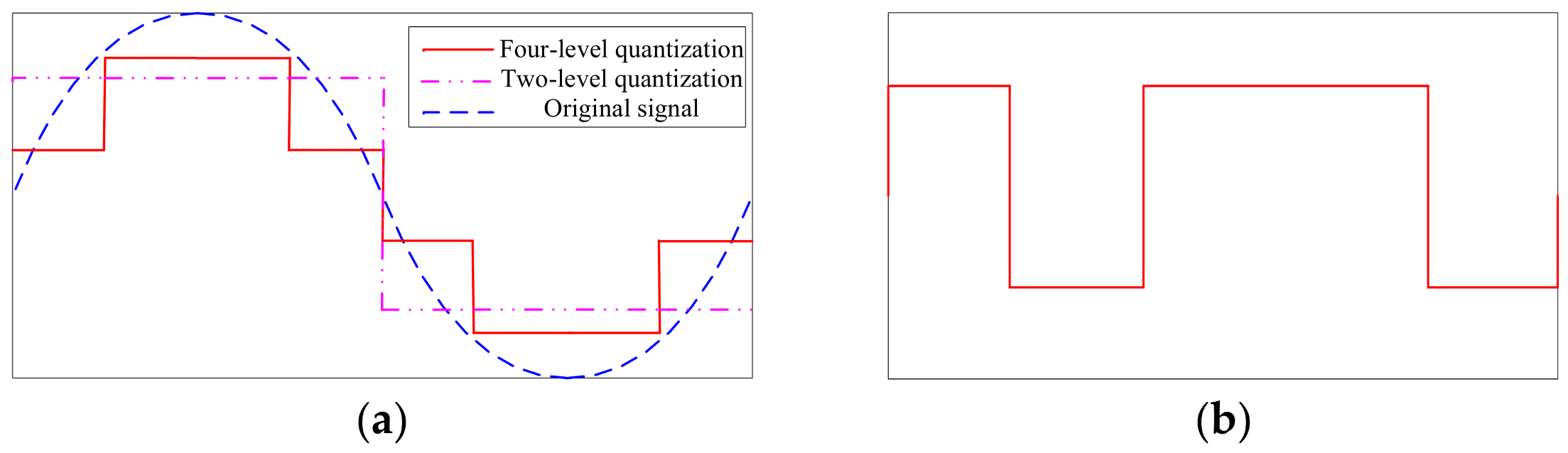
Generally, $s_i\left(t\right)$ is a binary sequence, and for digital circuit processing the carrier $e^{j2\pi \Delta f_{i}t}$ needs to be sampled and quantified, as shown in Figure 1 below.

Abbreviate $e^{j2\pi \Delta f_{i}t}{s}_i\left(t\right)$ as ${\tilde{s}}_i\left(t\right)$, and ${\tilde{s}}_i$ is the sampled and quantized signal of ${\tilde{s}}_i\left(t\right)$, which has ${\kappa }_i$ levels $\left\{{\tilde{L}}_1,{\tilde{L}}_2,\cdots ,{\tilde{L}}_i,\cdots ,{\tilde{L}}_{{\kappa }_i}\right\},{\tilde{L}}_i\in ℂ$. For N signals $\left\{{\tilde{s}}_1,{\tilde{s}}_2,\cdots ,{\tilde{s}}_N\right\}$, the ith signal state could be expressed as ${\left\{{\tilde{s}}_1,{\tilde{s}}_2,\cdots ,{\tilde{s}}_N\right\}}_i=\left\{K_{1i},K_{2i},\cdots ,K_{Ni}\right\}$, where $K_{ji}$ is one level of the ${\kappa }_j$, $K_{ji}\in \left\{{\tilde{L}}_1,{\tilde{L}}_2,\cdots ,{\tilde{L}}_i,\cdots ,{\tilde{L}}_{{\kappa }_i}\right\}$, and there are $H$ signal states in total, $i=1~H$.

For ${\tilde{s}}_i$, any two signals of N, such as ${\tilde{s}}_i$ and ${\tilde{s}}_j$, are required to be orthogonal. This means that the correlation result of ${\tilde{s}}_i$ and ${\tilde{s}}_j$ is 0. If the probability that ${\tilde{s}}_i$ selects level ${\tilde{L}}_k$ and ${\tilde{s}}_j$ selects level ${\tilde{L}}_m$ is $p_{k,m}$, then

$$Corr\left({\tilde{s}}_i,{\tilde{s}}_j\right)={\displaystyle \sum _H{p}_{k,m}{\tilde{L}}_k{\tilde{L}}_m^{\hspace{0.17em}*}}=0.$$

(4)

Define $c_i=a_i+j{b}_i=A_i{e}^{j\Delta {\varphi }_i}$, then

$$S_{SUM}={\displaystyle \sum _{i=1}^N{c}_i{\tilde{s}}_i},$$

(5)

where $c_i$ is the coefficient of the signal ${\tilde{s}}_i$, and $c_i\in ℂ$ is a complex number, which describes the amplitude and phase of the signal ${\tilde{s}}_i$.

Generally, the multiplexing signal $S_{SUM}$ would not be a constant envelop signal. To construct a constant envelope signal, an extra signal denoted as $E$ needs to be provided. Then the constant envelope signal could be expressed as:

$$S_{CE}=S_{SUM}+E={\displaystyle \sum _{i=1}^N{c}_i{\tilde{s}}_i+E}.$$

(6)

To get the signal ${\tilde{s}}_i$ at the receiver, the received signal needs to be correlated with ${\tilde{s}}_i$, which can be expressed as follows:

$$Corr\left(S_{CE},{\tilde{s}}_i\right)=Corr\left(c_i{\tilde{s}}_i,{\tilde{s}}_i\right)+Corr\left(E,{\tilde{s}}_i\right).$$

(7)

To avoid the interference of the extra signal to the receiving signal, the extra signal needs to be orthogonal to the receiving signal expressed as below:

$$Corr\left(E,{\tilde{s}}_i\right)=0.$$

(8)

This means that if the signal space is $\mathcal{S}$, $\forall {\tilde{s}}_i\in \mathcal{S}$, then the extra signal $E\in {\mathcal{S}}^{\perp }$ must be satisfied, where ${\mathcal{S}}^{\perp }$ is the orthogonal complement space of the signal space. The extra signal $E$ does not carry any information, it is only used to construct a constant envelope signal. Therefore, when the transmission power is limited, the lower the power of the extra signal, the higher the power of the useful signal transmitted. This means that the optimization goal is to construct a complete orthogonal complement space of the signal space, and select an extra signal $E$ with the lowest power from the space.

As the multiplexing signal is a phase modulation signal, different signal states will be mapped to different phases ${\left\{{\tilde{s}}_1,{\tilde{s}}_2,\cdots ,{\tilde{s}}_N\right\}}_i\to C{e}^{j{\theta }_i}$. To obtain a complete orthogonal complement space, construct a set of the following orthogonal basis:

$$l_i=\left\{\begin{array}{cc}1& {\left\{{\tilde{s}}_1,{\tilde{s}}_2,\cdots ,{\tilde{s}}_N\right\}}_i \mathrm{is} \mathrm{the} i{\mathrm{th}}^{} \mathrm{signal} \mathrm{state} \mathrm{of} H \\ 0& \mathrm{other} \mathrm{signal} \mathrm{states}\end{array}\right.,$$

(9)

where $i$ is from 1 to $H$. Then the constant envelope signal based on phase modulation could be described as:

$$S_{CE}=C{e}^{j{\theta }_1}{l}_1+C{e}^{j{\theta }_2}{l}_2+\cdots +C{e}^{j{\theta }_H}{l}_H=\theta l,$$

(10)

where ${\theta }_i$ is the ith phase mapping when ${\left\{{\tilde{s}}_1,{\tilde{s}}_2,\cdots ,{\tilde{s}}_N\right\}}_i$ is the ith signal state; $C$ is the constant modulus of those phase mapping; $\theta =\left[C{e}^{j{\theta }_1},C{e}^{j{\theta }_2},\cdots ,C{e}^{j{\theta }_H}\right]$ is the phase mapping vector; $l={\left[l_1,l_2,\cdots ,l_H\right]}^T$ is the phase orthogonal basis vector.

In order to understand the relationship between signal and phase mapping, make the following linear transformation:

$$s=\left[\begin{array}{c}\begin{array}{c}{\tilde{s}}_1\\ ⋮\\ {\tilde{s}}_N\end{array}\\ \begin{array}{c}{\tilde{e}}_{N+1}\\ ⋮\\ {\tilde{e}}_H\end{array}\end{array}\right]=\left[\begin{array}{cc}\begin{array}{ccc}{K}_{11}& \cdots & K_{1i}\\ ⋮& \ddots & ⋮\\ K_{N1}& \cdots & K_{Ni}\end{array}& \begin{array}{cc}\begin{array}{c}\cdots \\ \ddots \\ \cdots \end{array}& \begin{array}{c}{K}_{1H}\\ ⋮\\ K_{NH}\end{array}\end{array}\\ \begin{array}{ccc}{J}_{N+11}& \cdots & J_{N+1i}\\ ⋮& \ddots & ⋮\\ J_{H1}& \cdots & J_{Hi}\end{array}& \begin{array}{cc}\begin{array}{c}\cdots \\ \ddots \\ \cdots \end{array}& \begin{array}{c}{J}_{N+1H}\\ ⋮\\ J_{HH}\end{array}\end{array}\end{array}\right]\left[\begin{array}{c}\begin{array}{c}{l}_1\\ ⋮\\ l_N\end{array}\\ \begin{array}{c}{l}_{N+1}\\ ⋮\\ l_H\end{array}\end{array}\right]=Kl,$$

(11)

where $s={\left[{\tilde{s}}_1,\cdots ,{\tilde{s}}_N,{\tilde{e}}_{N+1},\cdots ,{\tilde{e}}_H\right]}^T$ is the vector describing the signals and the extra signals; $\tilde{s}=\left[{\tilde{s}}_1,\cdots ,{\tilde{s}}_N\right]$ describe $N$ signals and $e=\left[{\tilde{e}}_{N+1},\cdots ,{\tilde{e}}_H\right]$ describe $H-N$ extra signals; $K$ is the state matrix describing signal state. It can be seen from the definition of $l$ that ${\left\{{\tilde{s}}_1,\cdots ,{\tilde{s}}_N\right\}}_i=\left\{K_{1i},\cdots ,K_{Ni}\right\}$ is the ith signal state, and ${\left\{{\tilde{e}}_{N+1},\cdots ,{\tilde{e}}_H\right\}}_i=\left\{J_{N+1i},\cdots ,J_{Hi}\right\}$ at this time; $\left\{{\tilde{s}}_1,\cdots ,{\tilde{s}}_N\right\}$ is a set of complete orthogonal bases in the signal space $\mathcal{S}$, and $\left\{{\tilde{e}}_{N+1},\cdots ,{\tilde{e}}_H\right\}$ is a set of complete bases in the orthogonal complement space ${\mathcal{S}}^{\perp }$.

Then, the constant envelope multiplexing signal could be expressed as:

$$S_{CE}=\theta l=\theta K^{-1}s=cs,$$

(12)

where $\theta =\left[C{e}^{j{\theta }_1},C{e}^{j{\theta }_2},\cdots ,C{e}^{j{\theta }_H}\right]$ is the phase mapping vector; define $c=\theta K^{-1}$, and $c=\left[c_1,\cdots ,c_N,c_{N+1},\cdots ,c_H\right]$ are the coefficients of the signals and the extra signals. The constant envelope could be expressed as:

$$‖cK‖=‖\theta ‖=C,$$

(13)

where $‖•‖$ is the l₂-norm; $C$ is a constant, which can be normalized to 1, that’s $‖cK‖=‖\theta ‖=1$.

To maximize the power of the useful signal, it is necessary to select the coefficients of the extra signal that minimize the power of the extra signal. For DSSS constant envelope multiplexing signal, its power could be expressed as:

$$Corr\left(S_{CE},S_{CE}\right)=Corr\left(S_{SUM},S_{SUM}\right)+Corr\left(E,E\right),$$

(14)

where $Corr\left(•,•\right)$ is the correlation between the two signals; $S_{SUM}={\displaystyle \sum _{i=1}^N{c}_i{\tilde{s}}_i}$ is the signal; $E={\displaystyle \sum _{i=N+1}^H{c}_i{\tilde{e}}_i}$ is the extra signal. As the bases of extra signal space $\left\{{\tilde{e}}_{N+1},\cdots ,{\tilde{e}}_H\right\}$ are orthogonal to each other, there is no cross-correlation, and the power of constant multiplexing signal could be expressed as:

$$\begin{array}{ll}Corr\left(S_{CE},S_{CE}\right)& =Corr\left({\displaystyle \sum _{i=1}^N{c}_i{\tilde{s}}_i},{\displaystyle \sum _{i=1}^N{c}_i{\tilde{s}}_i}\right)+Corr\left({\displaystyle \sum _{i=N+1}^H{c}_i{\tilde{e}}_i},{\displaystyle \sum _{i=N+1}^H{c}_i{\tilde{e}}_i}\right)\\ & ={\displaystyle \sum _{i=1}^N‖c_i‖Corr\left({\tilde{s}}_i,{\tilde{s}}_i\right)}+{\displaystyle \sum _{i,j=1,i\ne j}^N{c}_i{c}_{j}Corr\left({\tilde{s}}_i,{\tilde{s}}_j\right)}+{\displaystyle \sum _{i=N+1}^H‖c_i‖Corr\left({\tilde{e}}_i,{\tilde{e}}_i\right)}+{\displaystyle \sum _{i,j=N+1,i\ne j}^H{c}_i{c}_{j}Corr\left({\tilde{e}}_i,{\tilde{e}}_j\right)}\\ & ={\displaystyle \sum _{i=1}^N‖c_i‖Corr\left({\tilde{s}}_i,{\tilde{s}}_i\right)}+{\displaystyle \sum _{i=N+1}^H‖c_i‖Corr\left({\tilde{e}}_i,{\tilde{e}}_i\right)}\end{array},$$

(15)

where ${\tilde{s}}_i$ and ${\tilde{s}}_j$ are orthogonal, $Corr\left({\tilde{s}}_i,{\tilde{s}}_j\right)=0$; ${\tilde{e}}_i$ and ${\tilde{e}}_j$ are orthogonal, $Corr\left({\tilde{e}}_i,{\tilde{e}}_j\right)=0$.

From the above description, for $N$ signals with H signal states, the method of constructing a multi-carrier constant envelope multiplexing signal is to find $H-N$ orthogonal bases in the extra signal space and select their coefficients to satisfy the following Equation (16):

$$\left\{\begin{array}{c}\left\{c_1,\cdots ,c_N\right\}\hspace{1em}\mathrm{decided} \mathrm{by} \mathrm{signals}\\ ‖cK‖=1\\ \max \left\{Corr\left(S_{SUM},S_{SUM}\right)/Corr\left(S_{CE},S_{CE}\right)\right\}\end{array}\right.,$$

(16)

where $\left\{{\theta }_1,\cdots ,{\theta }_H\right\}=\arg \left\{cK\right\}$ is the phase of different signal states.

The Equation (16) is actually a nonlinear constrained optimization problem. The objective function is $\left\{Corr\left(S_{SUM},S_{SUM}\right)/Corr\left(S_{CE},S_{CE}\right)\right\}$, and the constraint is $‖cK‖=1$. Any method of solving nonlinear constraint optimization can be used to solve the equation. One of the effective methods is the quasi-Newton algorithm based on penalty function, which construct the optimization function as follows:

$$\begin{array}{ll}\mathcal{F}& =\left(1-Corr\left(S_{SUM},S_{SUM}\right)/Corr\left(S_{CE},S_{CE}\right)\right)+\mu \left(‖cK‖-1\right)\\ & =\left(Corr\left(E,E\right)/Corr\left(S_{CE},S_{CE}\right)\right)+\mu \left(‖cK‖-1\right)\end{array},$$

(17)

where $\mu$ is the penalty factor. According to quasi-Newton method, find the minimum value of $\mathcal{F}$ and the coefficient vector $c$.

3. Constant Envelope Multiplexing Based on Probability and Homogeneous Equations

3.1. General Constuction Based on Probability and Homogeneous Equations

For binary signals, the method of constructing orthogonal bases is Inter-Modulation. There are N binary signals $s_1,s_2,s_3,\cdots ,s_i,\cdots s_N$, the Inter-Modulation to construct $2^N$ orthogonal bases is

$$\underset{C_N^0}{\underbrace{1}},\underset{C_N^1}{\underbrace{s_1,s_2,\cdots s_i,\cdots s_N}},\underset{C_N^2}{\underbrace{s_1{s}_2,s_1{s}_i,\cdots ,s_{N-1}{s}_N}},\underset{C_N^3}{\underbrace{s_1{s}_2{s}_3,\cdots }},\cdots ,\underset{C_N^N}{\underbrace{s_1{s}_2\cdots s_N}}$$

(18)

where $C_N^m$ is the number of m-combinations from a set of N elements. For multi-level signals, the orthogonal bases are constructed by Gram–Schmidt orthogonalization based on the Inter-Modulation. The method of multi-carrier constant envelope multiplexing method based on Inter-Modulation (CEMIM) first constructs a set of orthogonal bases in baseband code space and a set of orthogonal bases in subcarrier space, as shown in Equations (19) and (20) respectively.

$$s_{bb-code}=\left\{s_1,\cdots ,s_N,I{M}_{N+1},\cdots ,I{M}_{2^N}\right\},$$

(19)

$$s_{sub}=\left\{Q\left[e^{j2\pi \Delta f_{1}t}\right],\hspace{0.17em}\cdots ,Q\left[e^{j2\pi \Delta f_{N}t}\right],I{M}_{N+1},\cdots ,I{M}_F\right\},$$

(20)

where $s_{bb-code}$ are a set of orthogonal bases in baseband code space; $s_{sub}$ are a set of orthogonal bases in subcarrier space; $2^N$ and $F$ are the dimension of baseband code space and subcarrier space respectively; $IM$ is the Inter-Modulation; $Q\left[•\right]$ is quantization function. Then, the tensor product of two sets of orthogonal bases is used to construct the orthogonal base of multi-carrier signal space, as shown in Equation (21).

$$s=s_{bb-code}\otimes s_{sub}$$

(21)

However, the frequency constraint of the sub-carriers will affect the orthogonality of the orthogonal bases in Equation (20). At the same time, because the two sets of orthogonal bases are not considered uniformly, the construction of the orthogonal bases of the signal space by the tensor product will greatly increase the computational complexity. The signal states probability and homogeneous equations are introduced in this article to solve these problems.

Let ${\tilde{s}}_i\left(t\right)=e^{j2\pi \Delta f_{i}t}{s}_i\left(t\right)$, and after quantization, it can be expressed as:

$${\tilde{s}}_i=Q\left[e^{j2\pi \Delta f_{i}t}\right]s_i=Q\left[\cos \left(2\pi \Delta f_{i}t\right)\right]s_i+jQ\left[\sin \left(2\pi \Delta f_{i}t\right)\right]s_i,$$

(22)

where $Q\left[•\right]$ is quantization function. For N independent baseband code signals $s_1,s_2,\cdots ,s_N$ with M-level $\left\{L_1,-L_1,\cdots ,L_{M/2},-L_{M/2}\right\}$, $L_i\in ℝ$, there are $M^N$ baseband code states ${\left\{s_1=L_{j1},s_2=L_{j2},\cdots ,s_N=L_{jN}\right\}}_k$, $L_{ji}\in \left\{L_1,-L_1,\cdots ,L_{M/2},-L_{M/2}\right\}$, $k=1~M^N$, where $L_{ji}$ is the level of the ith code; $k$ is the kth baseband code state. Since sub-carriers are known signals with symmetry, after T-level quantization of N subcarriers $\left\{{\zeta }_1,-{\zeta }_1,\cdots ,{\zeta }_{T/2},-{\zeta }_{T/2}\right\}$, ${\zeta }_i\in ℂ$, there are F subcarrier states ${\left\{Q\left[e^{j2\pi \Delta f_{1}t}\right]={\zeta }_{j1},Q\left[e^{j2\pi \Delta f_{2}t}\right]={\zeta }_{j2},\cdots ,Q\left[e^{j2\pi \Delta f_{N}t}\right]={\zeta }_{jN}\right\}}_k$, ${\zeta }_{ji}\in \left\{{\zeta }_1,-{\zeta }_1,\cdots ,{\zeta }_{T/2},-{\zeta }_{T/2}\right\}$, $k=1~F$, where F is determined by the number of quantization levels and the subcarrier frequency constraint; ${\zeta }_{ji}$ is the level of the ith sub-carrier; $k$ is the kth sub-carrier state. The symmetry of the code and sub-carrier will make the value of the ith multiplexed signal equal in the following cases, ${\tilde{s}}_i=Q\left[e^{j2\pi \Delta f_{i}t}\right]s_i={\zeta }_{ji}{L}_{ji}=\left(-{\zeta }_{ji}\right)\left(-L_{ji}\right)$, so the dimension of the signal state space can be reduced. Define the kth valid sub-carrier state as:

$${\left\{\mathrm{ab}\left(Q\left[e^{j2\pi \Delta f_{1}t}\right]\right),\cdots ,\mathrm{ab}\left(Q\left[e^{j2\pi \Delta f_{N}t}\right]\right)\right\}}_k,$$

(23)

where $\mathrm{ab}\left(•\right)$ is that if ${\zeta }_i\in \left\{-{\zeta }_1,\cdots ,-{\zeta }_{T/2}\right\}$, then $\mathrm{ab}\left({\zeta }_i\right)=-{\zeta }_i$, else $\mathrm{ab}\left({\zeta }_i\right)={\zeta }_i$; $k=1~U$, and $U$ is the number of valid sub-carrier states in F sub-carrier states. Then the dimension of the signal state space is $H=U{M}^N$. For binary code, it would be $H=2^{N}U$.

One of the signal state probability is

$$P_i\left(\mathrm{ab}\left(Q\left[e^{j2\pi \Delta f_{1}t}\right]\right)s_1=L_{i1}{\zeta }_{j1},\cdots ,\mathrm{ab}\left(Q\left[e^{j2\pi \Delta f_{N}t}\right]\right)s_N=L_{iN}{\zeta }_{jN}\right),$$

(24)

where $L_{i1},\cdots ,L_{iN}\in \left\{L_1,-L_1,\cdots ,L_{M/2},-L_{M/2}\right\}$ and ${\zeta }_{j1},\cdots ,{\zeta }_{jN}\in \left\{{\zeta }_1,\cdots ,{\zeta }_{T/2}\right\}$. Using the principle of conditional probability, the probability of one signal state could be gotten:

$$\begin{gathered} P_i\left(\mathrm{ab}\left(Q\left[e^{j2\pi \Delta f_{1}t}\right]\right)s_1=L_{i1}{\zeta }_{j1},\cdots ,\mathrm{ab}\left(Q\left[e^{j2\pi \Delta f_{N}t}\right]\right)s_N=L_{iN}{\zeta }_{jN}\right) \\ =P_i\left(\mathrm{ab}\left(Q\left[e^{j2\pi \Delta f_{1}t}\right]\right)={\zeta }_{j1},\cdots ,\mathrm{ab}\left(Q\left[e^{j2\pi \Delta f_{N}t}\right]\right)={\zeta }_{jN}|s_1=L_{i1},\cdots ,s_N=L_{iN}\right)\cdot P\left(s_1=L_{i1},\cdots ,s_N=L_{iN}\right) \\ =P_i\left(\mathrm{ab}\left(Q\left[e^{j2\pi \Delta f_{1}t}\right]\right)={\zeta }_{j1},\cdots ,\mathrm{ab}\left(Q\left[e^{j2\pi \Delta f_{N}t}\right]\right)={\zeta }_{jN}|s_1=L_{i1},\cdots ,s_N=L_{iN}\right)\cdot P\left(s_1=L_{i1}\right)\cdots P\left(s_N=L_{iN}\right), \end{gathered}$$

(25)

where baseband codes $s_1,s_2,\cdots ,s_N$ are independent each other.

As there are $H$ signal states, $H-N$ orthogonal bases need to be constructed. Supposing a basis is $x=\left[x_1,x_2,\cdots ,x_H\right]$, it needs to be orthogonal with any signal ${\tilde{s}}_i$. The homogenous equations could be listed as follows:

$$\left\{\begin{array}{c}Corr\left({\tilde{s}}_i,x\right)=0,\hspace{1em}i=1~H-1\\ Corr\left(1,x\right)=0\hspace{1em}\hspace{1em}\hspace{1em}\hspace{1em}\hspace{1em}\hspace{1em}\end{array}\right.,$$

(26)

where $Corr({\tilde{s}}_i,x)={\displaystyle \sum _{i=1}^H{P}_i{\tilde{L}}_i}{x}_i$, ${\tilde{L}}_i=L_{ii}{\zeta }_{ji}$ is the ith value; $Corr\left(1,x\right)=0$ means that $x$ does not contain DC component. The solution space of the equations together with the space of DC component forms the signal orthogonal complement space. Solving the homogeneous linear equations and orthogonalize its solutions, the orthogonal bases could be gotten:

$$\left\{{\tilde{e}}_{N+1},\cdots ,{\tilde{e}}_H\right\}=\left\{1,so{l}_1,\cdots ,so{l}_{H-N-1}\right\}$$

(27)

where $so{l}_i$ is the ith solution vector. Using Equations (12) and (16) could get the constant envelope multiplexing signal. The algorithm to construct general multi-carrier constant envelope multiplexing signal based on probability and homogeneous equations (GCEMPH) is listed in Algorithm 1.

Algorithm 1: General construction based on probability and homogeneous equations

Input:$c_1{\tilde{s}}_1,c_2{\tilde{s}}_2,\cdots ,c_N{\tilde{s}}_N$

Output: GCEMPH signal

1 Determine the U valid sub-carrier states and H signal states according to the DSSS codes and sub-carriers;

2 According to Equation (25), find the probability of each signal states $P_i,\hspace{0.17em}i=1,\cdots ,H;$

3 According to homogeneous Equation (26) and orthogonal bases Equation (27) to find the H − N extra signals $\left\{{\tilde{e}}_{N+1},\cdots ,{\tilde{e}}_H\right\};$

4 GCEMPH signal $S_{CE}=S_{SUM}+E={\displaystyle \sum _{i=1}^N{c}_i{\tilde{s}}_i}+{\displaystyle \sum _{i=N+1}^H{c}_i{\tilde{e}}_i}$ , where $\left\{c_{N+1},\cdots ,c_H\right\}$ are the H − N unknowns;

5 According to Equations (15) and (16), use the optimization algorithms such as Equation (17) to find $\left\{c_1,\cdots ,c_H\right\}.$

3.2. Constuction Based on Probability and Homogeneous Equations without Sub-Carrier Interference

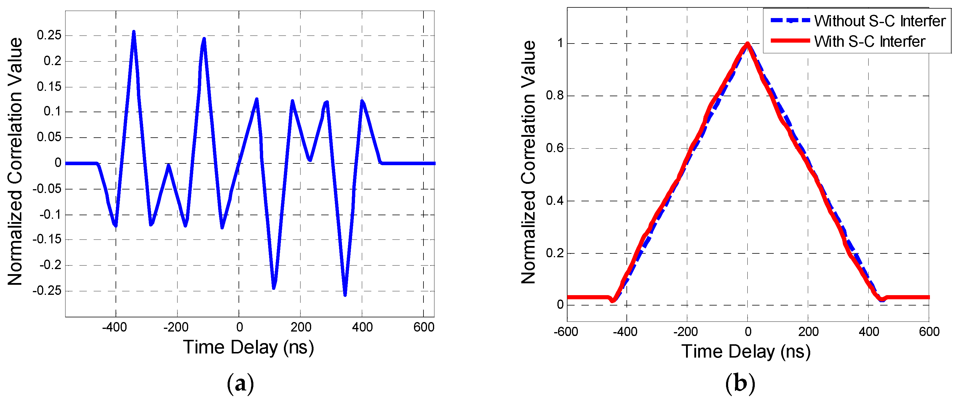
There are two orthogonal bases, they are signal $s_1(t)Q[\cos ({\omega }_{s}t)]$ and extra signal $s_1(t)Q[\cos ({\omega }_{s}t)]\cdot Q[\sin ({\omega }_{s}t)]$. The correlation result of the two bases will introduce interference as shown in Figure 2. The interference is actually introduced by the sub-carrier with the same PRN code, which is called sub-carrier (S-C) interference. Figure 2b shows the influence of S-C interference on the correlation curve, and it can be seen that it causes the distortion of the correlation curve.

The reason for generating the interference is the period of PRN code and sub-carrier are different. To eliminate the interference, the product of the subcarrier space bases $s_{sub}$ and the baseband codes $\left\{s_1,\cdots ,s_N\right\}$ cannot appear in the extra signal term, which means the orthogonal bases of the signal complement space is incomplete, and will lead to a reduction in multiplexing efficiency.

To get the constant envelope multiplexing signal without sub-carrier interference conveniently, an optimization method based on the combination of orthogonal basis and phase shift is proposed. There are N signals ${\tilde{s}}_1,{\tilde{s}}_2,\cdots ,{\tilde{s}}_N$, on which $s_1,s_2,\cdots ,s_N$ are baseband codes with M-level and sub-carrier signals have $U$ valid sub-carrier states ${\left\{\mathrm{ab}\left(Q\left[e^{j2\pi \Delta f_{1}t}\right]\right),\mathrm{ab}\left(Q\left[e^{j2\pi \Delta f_{2}t}\right]\right),\cdots ,\mathrm{ab}\left(Q\left[e^{j2\pi \Delta f_{N}t}\right]\right)\right\}}_k$, $k=1,\cdots ,U$, and the ith valid sub-carrier state probability is $P_i$. The baseband codes $s_1,s_2,\cdots ,s_N$ and their extra parts construct a group of orthogonal bases $\left\{s_1,\cdots ,s_N,e_{N+1},\cdots ,e_{M^N}\right\}$. Because the extra parts $\left\{e_{N+1},\cdots ,e_{M^N}\right\}$ are orthogonal to the baseband codes $\left\{s_1,\cdots ,s_N\right\}$, the baseband codes $\left\{s_1,\cdots ,s_N\right\}$ won’t appear in the extra parts. The N baseband code coefficients are $\left\{c_1,c_2,\cdots ,c_N\right\}$, $c_i\in ℂ$, then the constant envelope signals could be expressed as:

$$‖S_{CE}‖=‖c_1{s}_1\mathrm{ab}\left(Q\left[e^{j2\pi \Delta f_{1}t}\right]\right)+\cdots +c_N{s}_N\mathrm{ab}\left(Q\left[e^{j2\pi \Delta f_{N}t}\right]\right)+d_{N+1}{e}_{N+1}+\cdots +d_{M^N}{e}_{M^N}‖=1.$$

(28)

where $\left\{d_{N+1},\cdots ,d_{M^N}\right\}$ are the coefficients of the extra parts which varies with the value of $\left\{\mathrm{ab}\left(Q\left[e^{j2\pi \Delta f_{1}t}\right]\right),\cdots ,\mathrm{ab}\left(Q\left[e^{j2\pi \Delta f_{N}t}\right]\right)\right\}$. If the ith valid sub-carrier state is $\left\{\mathrm{ab}{\left(Q\left[e^{j2\pi \Delta f_{1}t}\right]\right)}_i,\cdots ,\mathrm{ab}{\left(Q\left[e^{j2\pi \Delta f_{N}t}\right]\right)}_i\right\}$, and the extra part coefficients in the ith valid sub-carrier state are $\left\{d_{N+1,i},\cdots ,d_{M^N,i}\right\}$, $d_i\in ℂ$. The constant envelope equations could be listed as:

$$\left\{\begin{array}{c}‖c_1{s}_1\mathrm{ab}{\left(Q\left[e^{j2\pi \Delta f_{1}t}\right]\right)}_1+\cdots +c_N{s}_N\mathrm{ab}{\left(Q\left[e^{j2\pi \Delta f_{N}t}\right]\right)}_1+d_{N+1,1}{e}_{N+1}+\cdots +d_{M^N,1}{e}_{M^N}‖=1\\ ⋮\\ ‖c_1{s}_1\mathrm{ab}{\left(Q\left[e^{j2\pi \Delta f_{1}t}\right]\right)}_U+\cdots +c_N{s}_N\mathrm{ab}{\left(Q\left[e^{j2\pi \Delta f_{N}t}\right]\right)}_U+d_{N+1,U}{e}_{N+1}+\cdots +d_{M^N,U}{e}_{M^N}‖=1\end{array}\right..$$

(29)

If the amplitude ratio of the baseband code is $A_1:A_2:\cdots :A_N=1:{\alpha }_2:\cdots :{\alpha }_N$, then the amplitude of the N signals could be expressed as $\left\{A_1=a,A_2={\alpha }_{2}a,\cdots ,A_N={\alpha }_{N}a\right\}$, where $a$ is an unknown. If the phase relationship of N baseband code is $\left\{e^{j{\phi }_1},e^{j{\phi }_2},\cdots ,e^{j{\phi }_N}\right\}$, then the baseband code coefficients are $\left\{c_1,c_2,\cdots ,c_N\right\}=\left\{a{e}^{j{\phi }_1},{\alpha }_{2}a{e}^{j{\phi }_2},\cdots ,{\alpha }_{N}a{e}^{j{\phi }_N}\right\}$. Optimization $\left\{a,d_{N+1,1},\cdots ,d_{M^N,1},\cdots ,d_{N+1,U},\cdots ,d_{M^N,U}\right\}$, to get the maximum of multiplexing efficiency:

$$P_1\frac{Corr\left(S_1,S_1\right)}{Corr\left(S_1+E_1,S_1+E_1\right)}+\cdots +P_U\frac{Corr\left(S_U,S_U\right)}{Corr\left(S_U+E_U,S_U+E_U\right)},$$

(30)

where $S_i=c_1{s}_1\mathrm{ab}{\left(Q\left[e^{j2\pi \Delta f_{1}t}\right]\right)}_i+\cdots +c_N{s}_N\mathrm{ab}{\left(Q\left[e^{j2\pi \Delta f_{N}t}\right]\right)}_i$, $E_i=d_{N+1,i}{e}_{N+1}+\cdots +d_{M^N,i}{e}_{M^N}$.

Taking Equation (30) as the objective function and Equation (29) as the constraint, those unknown could be easily obtained by using the nonlinear constrained optimization algorithm, such as the quasi-Newton method based on the penalty function.

Actually, the AltBoc modulation used in the Galileo System can be seen as a special case of this method. The algorithm to construct multi-carrier constant envelope multiplexing signal based on probability and homogeneous equations no sub-carrier interference (CEMPHNSI) is listed in Algorithm 2.

Algorithm 2: Construction based on probability and homogeneous equations without sub-carrier interference

Input:$c_1{s}_1,c_2{s}_2,\cdots ,c_N{s}_N, \left\{Q\left[e^{j2\pi \Delta f_{1}t}\right],Q\left[e^{j2\pi \Delta f_{2}t}\right],\cdots ,Q\left[e^{j2\pi \Delta f_{N}t}\right]\right\}$

Output: CEMPHNSI signal

1 Determine the baseband code states $M^N$ and the valid sub-carrier states U;

2 Find the probability of each valid sub-carrier state $P_i,\hspace{0.17em}i=1,\cdots ,U;$

3 According to homogeneous Equation (26) or Inter-modulation Equation (18) to find the $M^N-N$ extra signals $\left\{e_{N+1},\cdots ,e_{M^N}\right\};$

4 According to Equations (29) and (30), find the coefficients of extra parts $\left\{d_{N+1,i},\cdots ,d_{M^N,i}\right\}$ and signals $\left\{c_1,c_2,\cdots ,c_N\right\}$ by the optimization algorithm;

5 CEMPHNSI signal:

$S_{CE}=c_1{s}_1\mathrm{ab}{\left(Q\left[e^{j2\pi \Delta f_{1}t}\right]\right)}_i+\cdots +c_N{s}_N\mathrm{ab}{\left(Q\left[e^{j2\pi \Delta f_{N}t}\right]\right)}_i+d_{N+1,i}{e}_{N+1}+\cdots +d_{M^N,i}{e}_{M^N}.$

4. Constant Envelope Multiplexing of Three Different Frequency Signals

There are three independent binary DSSS signals $s_1,s_2,s_3$ with code frequency $2.046$ MHz and BPSK(2) modulation:

$$s_i={\displaystyle \sum _{k=-\infty }^{\infty }cod{e}_i{\psi }_{T_c}\left(t-k{T}_c\right)},$$

(31)

where $cod{e}_i$ is the PRN code of the ith signal $s_i$, its value is 1 or −1; ${\psi }_{T_c}$ is the duration of each chip and the code frequency is $f_c=1/T_c=2.046$ MHz. The amplitude ratio of the three signals is $A_{s_1}:A_{s_2}:A_{s_3}=1:1:1$, and the phase relationship is $\left\{P{h}_{s_1},P{h}_{s_2},P{h}_{s_3}\right\}=\left\{e^{j0},e^{j0},e^{j\pi /2}\right\}$. $s_1$ has a frequency offset $e^{j{\omega }_{s}t}$ from the center frequency, $s_2$ has the frequency offset $e^{-j3{\omega }_{s}t}$ from the center frequency, and $s_3$ has no frequency offset, where ${\omega }_s=2\pi f_s$ and $f_s=4.092$ MHz.

According to the principle of constant envelope multiplexing, the CE signal could be expressed as:

$$\begin{gathered} S_{CE}=a_1{s}_1{e}^{j{\omega }_{s}t}+a_1{s}_2{e}^{-j3{\omega }_{s}t}+j{a}_1{s}_3+E \\ =\left(a_1{s}_1\cos \left({\omega }_{s}t\right)+a_1{s}_2\cos \left(3{\omega }_{s}t\right)+S_{extra-I}\right)+j\left(a_1{s}_1\sin \left({\omega }_{s}t\right)-a_1{s}_2\sin \left(3{\omega }_{s}t\right)+a_1{s}_3+S_{extra-Q}\right), \end{gathered}$$

(32)

where $S_{extra-I}$ is the in-phase component of the extra signal and $S_{extra-Q}$ is the quadrature-phase component of the extra signal; the coefficients of signals are $c_1=a_1,c_2=a_1,c_3=j{a}_1$ decided by amplitude and phase relationship. After two-level quantization, the sub-carrier could be expressed as follows:

$$\begin{array}{l}s{c}_{c-{\omega }_s}=\mathrm{sign}\left[\cos \left({\omega }_{s}t\right)\right],\hspace{1em}s{c}_{s-{\omega }_s}=\mathrm{sign}\left[\sin \left({\omega }_{s}t\right)\right]\\ s{c}_{c-3{\omega }_s}=\mathrm{sign}\left[\cos \left(3{\omega }_{s}t\right)\right],\hspace{0.17em}s{c}_{s-3{\omega }_s}=\mathrm{sign}\left[\sin \left(3{\omega }_{s}t\right)\right]\end{array},$$

(33)

then the multiplexing signal could be expressed as follows:

$$S_{CE}=\left(a_1{s}_{1}s{c}_{c-{\omega }_s}+a_1{s}_{2}s{c}_{c-3{\omega }_s}+S_{extra-I}\right)+j\left(a_1{s}_{1}s{c}_{s-{\omega }_s}-a_1{s}_{2}s{c}_{s-3{\omega }_s}+a_1{s}_3+S_{extra-Q}\right).$$

(34)

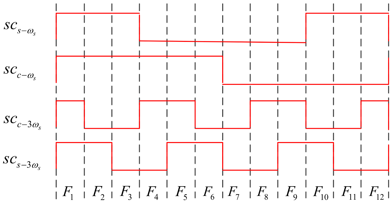
For the 3 multiplexed signals, there are $2^3=8$ baseband code states and $F=12$ sub-carrier states. The sub-carrier states are decided by the frequency constraint and quantization level as shown in Figure 3. The probability of each code state is $P_{C_i}=1/8$ and the probability of each sub-carrier state is $P_{F_i}=1/12$.

According to the definition of valid sub-carrier states, there are only four valid sub-carrier states in the 12 sub-carrier states, they are $U_1:\left\{1+j,1+j,1\right\}$, $U_2:\left\{1+j,-1+j,1\right\}$, $U_3:\left\{-1+j,-1+j,1\right\}$, and $U_4:\left\{-1+j,1+j,1\right\}$, the probability of valid sub-carrier states are $P_{U_1}=1/3$, $P_{U_2}=1/6$, $P_{U_3}=1/3$ and $P_{U_4}=1/6$, respectively. Where ${\zeta }_1=1+j$, $-{\zeta }_1=-1-j$, ${\zeta }_2=-1+j$ and $-{\zeta }_2=1-j$. The number of signal states is $H=2^3\cdot 4=32$ in total. The probability of one of the signal states is

$$\begin{array}{l}{P}_1=P\left(s_{1}s{c}_{c-{\omega }_s}=1,s_{1}s{c}_{s-{\omega }_s}=1,s_{2}s{c}_{c-3{\omega }_s}=1,s_{2}s{c}_{s-3{\omega }_s}=1,s_3=1\right)\\ \hspace{1em}=P\left(U_1|s_1=1,s_2=1,s_3=1\right)P\left(s_1=1,s_2=1,s_3=1\right)=1/24\end{array}$$

(35)

and other probability of the signal states could be gotten as well. From homogeneous Equation (26) and orthogonal bases Equation (27) the extra signals could be gotten and from Equations (16) and (17) the coefficients of extra signals could be gotten.

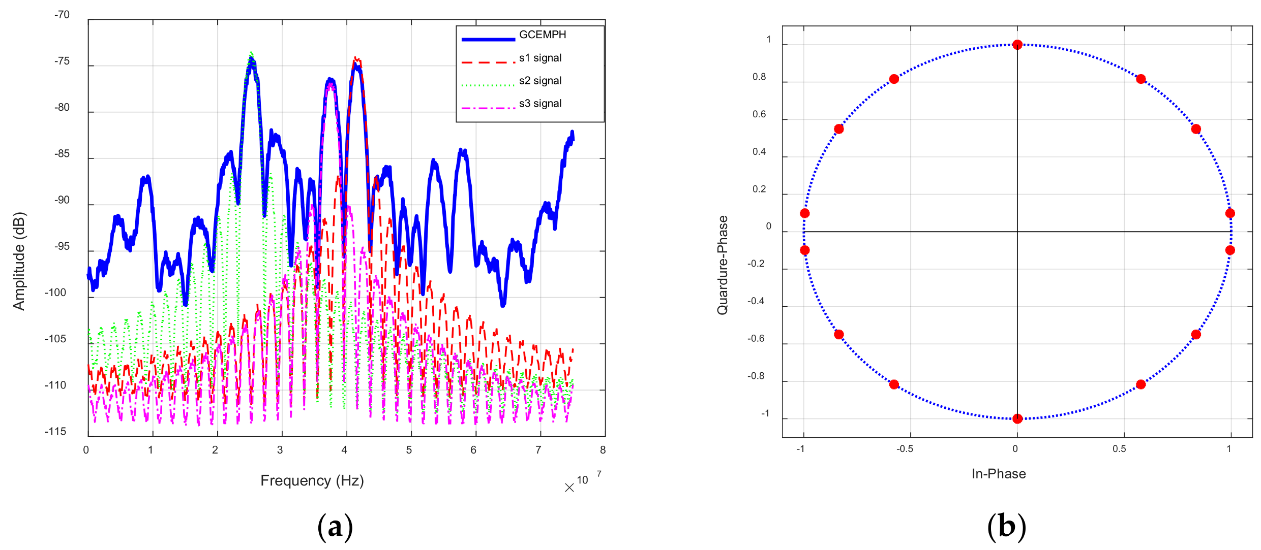
After optimization, the GCEMPH could be gotten, and according to Equations (16) and (17), its multiplexing efficiency is 83.88%. The Figure 4 provides the power spectrum and the constellation of GCEMPH.

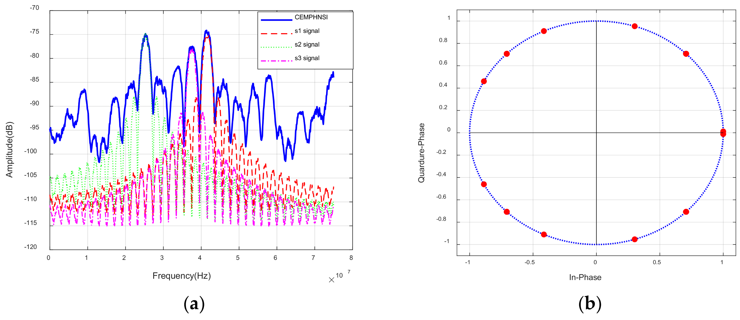
According to Algorithm 2, the CEMPHNSI could be gotten, and its multiplexing efficiency is 62.50%. The Figure 5 provides the power spectrum and the constellation of CEMPHNSI. Compared with GCEMPH, its multiplexing efficiency is reduced by 21.38%, which is the price paid for not introducing sub-carrier interference.

5. Multiplexing Signal Analysis

5.1. Receiving Correlation Results and Power Ratio

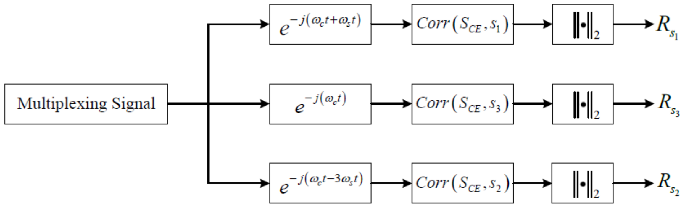
The receiving module of constant envelope multiplexing signal is shown in Figure 6.

The normalized cross-correlation between the ith signal and the multiplexing signal is defined as:

$$R_{s_i}\left(\tau \right)=\left|Corr\left(S_{CE}\left(t\right),s_i\left(t+\tau \right)\right)\right|/\max \left[Corr\left(s_i,s_i\right)\right].$$

(36)

And the normalized cross-correlation between the ith signal and the extra signal is defined as:

$$R_{(E,s_i)}\left(\tau \right)=\left|Corr\left(E\left(t\right),s_i\left(t+\tau \right)\right)\right|/\max \left[Corr\left(s_i,s_i\right)\right]$$

(37)

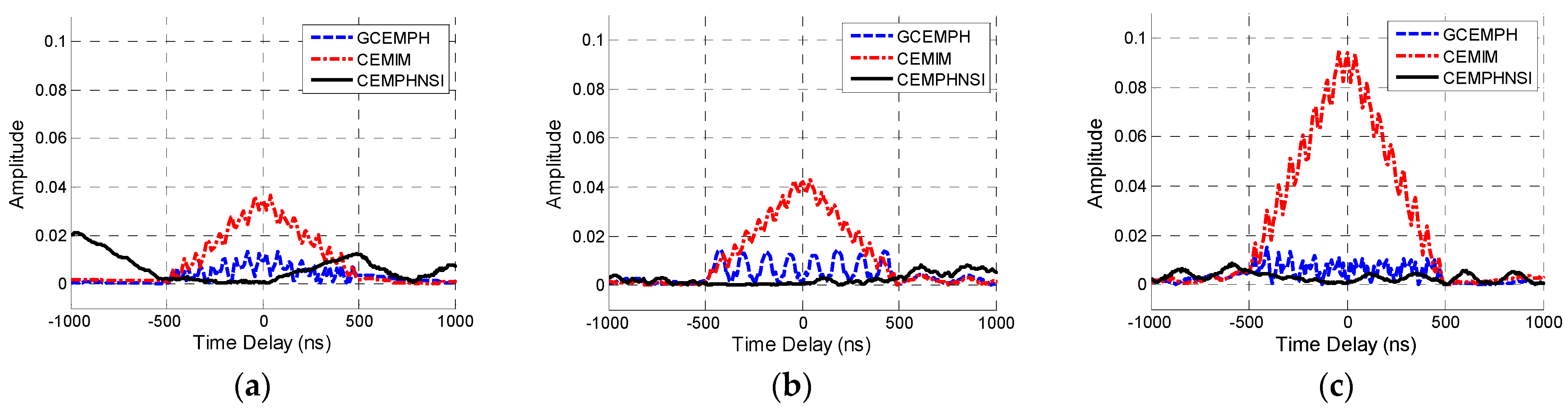
Figure 7a shows the normalized cross-correlation results of $s_1$ and three multiplexing signals. The three multiplexing signals are implemented using CEMIM, GCEMPH and CEMPHNSI methods, respectively. Figure 7b shows the normalized cross-correlation results of $s_2$ and three multiplexing signals; Figure 7c shows the normalized cross-correlation results of $s_3$ and three multiplexing signals. Figure 8a shows the normalized cross-correlation results of $s_1$ and three extra signals. The three extra signals are extra parts of CEMIM, GCEMPH and CEMPHNSI, respectively. Figure 8b shows the normalized cross-correlation results of $s_2$ and three extra signals; Figure 7c shows the normalized cross-correlation results of $s_3$ and three extra signals. In Figure 7, the maximum correlation result of CEMPHNSI is lower than GCEMPH that because the multiplexing efficiency of CEMPHNSI is lower than GCEMPH. In Figure 7c, the maximum correlation result of CEMIM has a noticeable drop, the reason is CEMIM has power leakage shown in Figure 8c and it is negatively correlated with the correlation result. From Figure 8, it can be seen that the CEMIM has more power leakage in extra signal compared with GCEMPH proposed in this paper, and GCEMPH and CEMIM all introduced sub-carrier interference compared with CEMPHNSI.

The receiving power ratio of the three signals could be expressed as:

$$P_{s_1}:P_{s_2}:P_{s_3}=\max \left[R_{s_1}\right]:\max \left[R_{s_2}\right]:\max \left[R_{s_3}\right].$$

(38)

Due to the influence of the quantization, the receiving signal power of a designed signal is $P_{s_1}:P_{s_2}:P_{s_3}=1:1:0.79$. The receiving power ratio of the three situations and designed situation are listed in

Table 1. The receiving power ratio of different multiplexing signal and of designed signal.

Different Situation	The Receiving Power Ratio
Design	$P_{s_1}:P_{s_2}:P_{s_3}=1:1:0.79$
GCEMPH	$P_{s_1}:P_{s_2}:P_{s_3}=1:1.01:0.80$
CEMIM	$P_{s_1}:P_{s_2}:P_{s_3}=1:1.01:0.64$
CEMPHNSI	$P_{s_1}:P_{s_2}:P_{s_3}=1:1:0.79$

, respectively.

From Table 1, the received power ratio of GCEMPH and CEMPHNSI is the same as the designed power ratio. Due to the power leakage, the received power ratio of CEMIM is different from the designed power ratio and is smaller than the design power ratio.

5.2. S-Curve Bias and Slope

Define the normalized cross-correlation-function (CCF) as [21]:

$$CCF\left(S_{CE},s_i,\tau \right)=\frac{Corr\left(S_{CE},s_i,\tau \right)}{\sqrt{Corr\left(S_{CE},S_{CE},0\right)}\cdot \sqrt{Corr\left(s_i,s_i,0\right)}},$$

(39)

Then the normalized S-Curve with early-late spacing $\delta$ is given by [21]:

$$SC\left(S_{CE},s_i,\tau \right)={\left|CCF\left(S_{CE},s_i,\tau +\delta /2\right)\right|}^2-{\left|CCF\left(S_{CE},s_i,\tau -\delta /2\right)\right|}^2.$$

(40)

With the smallest zero-crossing of the S-Curve ${\tau }_0$ according to the S-Curve bias, the relative change of S-Curve slope “dSlope”, relative to the ideal S-Curve slope for the undistorted signal is given by:

$$dSlope\left(S_{CE},s_i,{\tau }_0\right)=1-\frac{dSC\left(S_{CE},s_i,{\tau }_0\right)/d\tau }{dSC\left(s_i,s_i,0\right)/d\tau }.$$

(41)

Generally, the cross-correlation function affects the S-Curve bias and slope. In practical applications, the cross-correlation function will not be zero, so the S-Curve bias will be introduced, but it should not be too large. Otherwise, it will affect the ranging performance. In order to measure the influence of extra signals on the S-Curve bias and slope, define the S-Curve bias introduced by extra signals as:

$$SC\left(E,s_i,\tau \right)=SC\left(S_{CE},s_i,\tau \right)-SC\left(S_{SUM},s_i,\tau \right),$$

(42)

and the S-Curve slope introduced by extra signals as:

$$dSlope\left(E,s_i,{\tau }_0\right)=dSlope\left(S_{CE},s_i,{\tau }_0\right)-dSlope\left(S_{SUM},s_i,{\tau }_0\right).$$

(43)

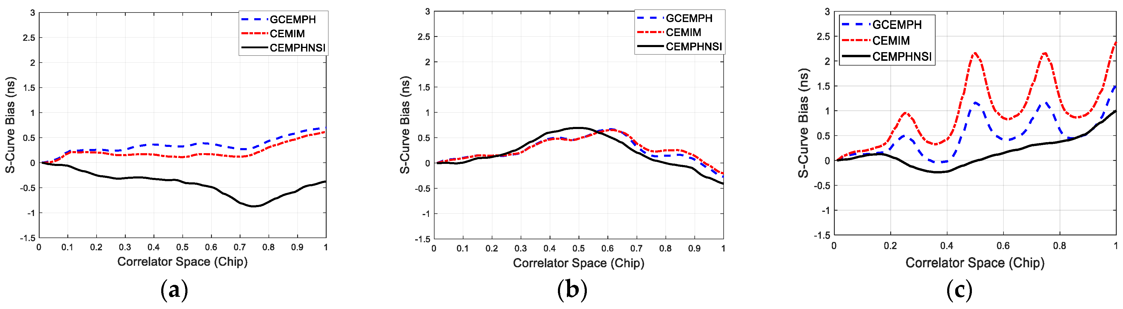
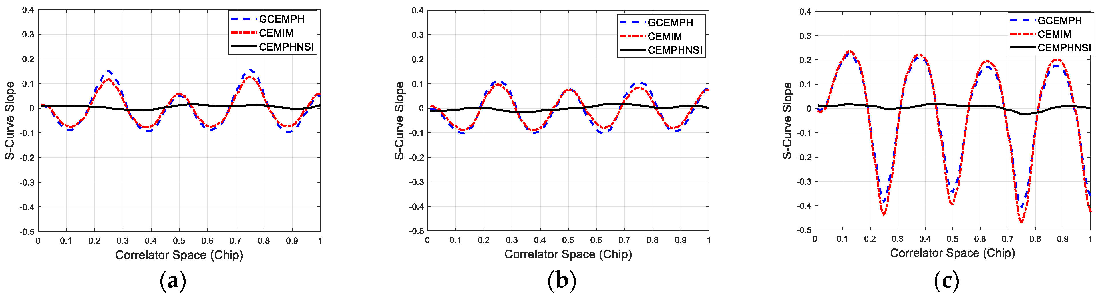
Figure 9 and Figure 10 provides the S-Curve bias and slope of 3 multiplexing signals introduced by extra signal, respectively. From Figure 9, it can be seen that the S-Curve bias of the $s_1$ and $s_2$ are no more than 1 ns, while for the $s_3$, the CEMIM introduces the more S-Curve bias compared with GCEMPH and CEMPHNSI, which more than 2 ns, that because the CEMIM has more power leakage. From Figure 10, it can be seen that the sub-carrier interference will cause the S-Curve slope fluctuations, and because the CEMPHNSI doesn’t have sub-carrier interference, it won’t introduce the S-Curve slope fluctuations.

5.3. Computational Complexity

As mentioned before, the dimension of the baseband code space is $2^3=8$ and the dimension of the sub-carrier space is $F=12$. The number of valid sub-carrier states is $U=4$. As the signal space dimension of CEMIM is based on the tensor product, then it would be $H=2^{3}F=96$. The GCEMPH and CEMPHSI are based on homogenous equations, they uniformly consider code space and sub-carrier space, the signal space dimension of them are $H=2^{3}U=32$.

The signals to be multiplexed are provided in Section 4.

Table 2. The number of optimization equations for different multiplexing methods.

Multiplexing Method	The Number of Optimization Equations
CEMIM	96
GCEMPH	32
CEMPHNSI	32

shows the number of optimization equations for 3 multiplexing methods.

From Table 2, it can be seen that the GCEMPH and CEMPHNSI proposed in this paper has much less number optimization equations than CEMIM, which greatly reduces the computational complexity in the orthogonal basis and optimization solution.

6. Conclusions

Flexible construction of diverse signals is the trend of next-generation satellite navigation systems. On the basis of the previous constant envelope multiplexing methods, this article considers the influence of the sub-carriers frequency constraint on the signal states probability of multi-carrier constant envelope multiplexing, and proposed multi-carrier constant envelope multiplexing methods based on probability and homogeneous equations including GCEMPH and CEMPHNSI. The analysis results reveal that, compared with previous methods, the methods can easily multiplex signals with any adjacent frequency offset and multiplex multi-carrier signals without power leakage, thereby reducing the impact on signal ranging performance. Meanwhile, the methods could reduce the computation complexity. Furthermore, compared with GCEMPH, CEMPHNSI could not introduce the sub-carrier interference, while its multiplexing efficiency is less than GCEMPH.

References

- Dunn, M.J. Global Positioning Systems Directorate Systems Engineering & Integration, Interface Specification (IS-GPS-200), NAVSTAR GPS Space Segment/Navigation User Segment Interfaces; IRN-IS-200H; GPS Directorate: Los Angeles, CA, USA, 2014. [Google Scholar]
- European Union. European GNSS (Galileo) Open Service Signal in Space Interface Control Document (GAL OS SIS ICD), Issue 1.3; European Commission: Strateburgum, France, 2016. [Google Scholar]
- China Satellite Navigation Office. BeiDou Navigation Satellite System Signal in Space Interface Control Document Open Service Signal B2a, 1st ed.; China Satellite Navigation Office: Beijing, China, 2017. [Google Scholar]
- United Nations. Current and Planned Global and Regional Navigation Satellite Systems and Satellite-Based Augmentations Systems. In Proceedings of the International Committee on Global Navigation Satellite Systems Provider’s Forum, New York, NY, USA, 7 June 2010; pp. 35–40. [Google Scholar]
- Yuan, G.Y.; Gang, W.; Jun, X. Assessing impact of payload non-linear distortion on CBOC signal. Space Electron. Technol. 2014, 58–62. [Google Scholar] [CrossRef]
- Elliott, D.K.; Christopher, J.H. Understanding GPS Principles and Applications, 2nd ed.; Publishing House of Electronics Industry: Beijing, China, 2012; pp. 81–85. [Google Scholar]
- Butman, S.; Timor, U. Interplex: An effificient multichannel PSK/PM telemetry system. IEEE Trans. Commun. Technol. 1972, 20, 415–419. [Google Scholar] [CrossRef]
- Dafesh, P.A.; Nguyen, T.M.; Lazar, S. Coherent adaptive subcarrier modulation (CASM) for GPS modernization. In Proceedings of the 1999 National Technical Meeting of the Institute of Navigation, San Diego, CA, USA, 25–27 January 1999; pp. 649–660. [Google Scholar]
- Spilker, J.J.; Orr, R.S. Code multiplexing via majority logic for GPS modernization. In Proceedings of the 1th International Technical Meeting of the Satellite Division of the Institute of Navigation (ION GPS 1998), Nashville, TN, USA, 15–18 September 1998; pp. 265–273. [Google Scholar]
- Cangiani, G.L.; Orr, R.S.; Nguyen, C.Q. Methods and Apparatus for Generating a Constant-Envelope Composite Transmission Signal. U.S. Patent 7,154,962, 26 December 2006. [Google Scholar]
- Dafesh, P.A.; Cahn, C.R. Phase-optimized constant-envelope transmission (POCET) modulation method for GNSS signals. In Proceedings of the 22nd International Technical Meeting of the Satellite Division of the Institute of Navigation (ION GNSS 2009), Savannah, GA, USA, 22–25 September 2009; pp. 2860–2866. [Google Scholar]
- Zhang, K.; Zhou, H.; Wang, F. Unbalanced AltBOC: A Compass B1 candidate with generalized MPOCET technique. GPS Solut. 2013, 17, 153–164. [Google Scholar] [CrossRef]
- Zhang, X.; Zhang, X.; Yao, Z.; Lu, M. Implementations of constant envelope multiplexing based on extended Interplex and inter-modulation construction method. In Proceedings of the 25th International Technical Meeting of the Satellite Division of the Institute of Navigation (ION GNSS 2012), Nashville, TN, USA, 17–21 September 2012; pp. 893–900. [Google Scholar]
- Lestarquit, L.; Artaud, G.; Issler, J.L. AltBOC for dummies or everything you always wanted to know about AltBOC. In Proceedings of the 21st International Technical Meeting of the Satellite Division of the Institute of Navigation (ION GNSS 2008), Savannah, GA, USA, 16–19 September 2008; pp. 961–970. [Google Scholar]
- Nagaraj, C.S.; Andrew, G.D. The Galileo E5 AltBOC: Understanding the signal structure. International global navigation satellite systems. In Proceedings of the Society IGNSS Symposium, Holiday Inn Surfers Paradise, Gold Coast, QLD, Australia, 1–3 December 2009. [Google Scholar]
- Tang, Z.; Zhou, H.; Wei, J. TD-AltBOC: A new COMPASS B2 modulation. Sci. China Phys. Mech. Astron. 2011, 54, 1014–1021. [Google Scholar] [CrossRef]
- Yao, Z.; Zhang, J.; Lu, M. ACE-BOC: Dual-frequency constant envelope multiplexing for satellite navigation. IEEE Trans. Aerosp. Electron. Syst. 2016, 52, 466–485. [Google Scholar] [CrossRef]
- Dafesh, P.A.; Cahn, C.R. Application of POCET method to combine GNSS signals at different carrier frequencies. In Proceedings of the 2011 International Technical Meeting of the Institute of Navigation, San Diego, CA, USA, 21–26 January 2011; pp. 1201–1206. [Google Scholar]
- Yao, Z.; Guo, F.; Ma, J.; Lu, M. Orthogonality-based generalized multicarrier constant envelope multiplexing for DSSS signals. IEEE Trans. Aerosp. Electron. Syst. 2017, 53, 1685–1697. [Google Scholar] [CrossRef]
- Ma, J.; Yao, Z.; Lu, M. Multicarrier constant envelope multiplexing technique by subcarrier vectorization for new generation GNSS. IEEE Commun. Lett. 2019, 23, 991–994. [Google Scholar] [CrossRef]
- Soellner, M.; Kohl, R.; Luetke, W. The impact of linear and non-linear signal distortions on Galileo code tracking accuracy. Pac. J. Math. 2002, 162, 27–44. [Google Scholar]
Figure 1.
(a) Four-level and two-level quantization within one cycle of the carrier, respectively; (b) The binary sequence of DSSS signal.
Figure 2.
(a) The S-C interference of and ; (b) The influence of S-C interference on the correlation curve.
Figure 3.
The sub-carrier state of the multiplexing signal.
Figure 4.
(a) The spectrum of GCEMPH and multiplexed signals; (b) The constellation of GCEMPH.
Figure 5.
(a) The spectrum of CEMPHNSI and multiplexed signals; (b) The constellation of CEMPHNSI.
Figure 6.
The receive module of the constant envelope multiplexing signal in Section 4.
Figure 7.
(a) The correlation between 3 multiplexing signals and signal s1; (b) The correlation between 3 multiplexing signals and signal s2; (c) The correlation between 3 multiplexing signals and signal s3.
Figure 8.
(a) The correlation between 3 extra signals and signal s1; (b) The correlation between 3 extra signals and signal s2; (c) The correlation between 3 extra signals and signal s3.
Figure 9.
(a) The S-Curve bias of 3 multiplexing signals with signal s1; (b) The S-Curve bias of 3 multiplexing signals with signal s2; (c) The S-Curve bias of 3 multiplexing signals with signal s3.
Figure 10.
(a) The S-Curve slope of 3 multiplexing signals with signal s1; (b) The S-Curve slope of 3 multiplexing signals with signal s2; (c) The S-Curve slope of 3 multiplexing signals with signal s3.