Article

Adaptive Sliding Mode Neural Network Control and Flexible Vibration Suppression of a Flexible Spatial Parallel Robot

1
School of Computer Science and Engineering, Tianjin University of Technology, Tianjin 300384, China
2
Tianjin Key Laboratory for Advanced Mechatronic System Design and Intelligent Control, National Demonstration Center for Experimental Mechanical and Electrical Engineering Education, Tianjin University of Technology, Tianjin 300384, China
*
Author to whom correspondence should be addressed.
Submission received: 4 December 2020 / Revised: 15 January 2021 / Accepted: 15 January 2021 / Published: 18 January 2021

Abstract

:
With the goal of creating a flexible spatial parallel robot system in which the elastic deformation of the flexible link causes a rigid moving platform to produce small vibrations, we proposed an adaptive sliding mode control algorithm based on a neural network. To improve the calculation efficiency, the finite element method was used to discretize the flexible spatial link, and then the displacement field of the flexible spatial link was described based on floating frame of reference coordinates, and the dynamic differential equation of the flexible spatial link considering high-frequency vibrations was established through the Lagrange equation. This was combined with the dynamic equation of the rigid link and the dynamic equation considering small displacements of the rigid movable platform due to elastic deformation, and a highly nonlinear and accurate dynamic model with a rigid–flexible coupling effect was obtained. Based on the established accurate multi-body dynamics model, the driving torque with coupling effects was calculated in advance for feedforward compensation, and the adaptive sliding mode controller was used to improve the tracking performance of the system. The nonlinear error was examined to determine the performance of the neural network’s approximation of the nonlinear system. The trajectory errors of the moving platform in the X-, Y-, and Z-directions were reduced by 12.1%, 38.8%, and 50.34%, respectively. The results showed that the designed adaptive sliding mode neural network control met the control accuracy requirements, and suppressed the vibrations generated by the deformation of the flexible spatial link.

1. Introduction

Parallel robots exhibit good dynamic performance, small cumulative errors, and fast response speeds. They are widely used in equipment manufacturing, aviation, precision machining, and other fields [1,2,3]. As the development of parallel robots has tended toward high speeds and low weights, the flexible deformation in the system has a significant influence on the accuracy of trajectory tracking. Therefore, determining how to improve the precise control of the trajectory and suppress the vibrations generated by the flexible deformation has become a popular subject of study in flexible parallel robots [4,5,6,7]. The elastic deformation and vibrations caused by the link and joint flexibility are important factors that affect the accuracy and stability of the system’s trajectory. Most of the current research focuses on the analysis of joint flexibility [8,9,10,11], but there has been less analysis of the flexibility of the robot arm [12,13,14]. In one study, the control problems of rigid–flexible coupled spatial manipulators using a wavelet fuzzy neural network were analyzed [15]. Yang et al. [16] applied a nonlinear proportional–derivative (PD) algorithm to study the control strategy of the self-excited vibrations caused by large deformations of the flexible link in the parallel mechanism. Zhang et al. [17] used a hybrid control algorithm with a PD feedback controller and strain rate feedback (SRF) controller to actively control the vibrations of a flexible parallel platform. However, the above research mainly adopted hypothetical modal methods to describe the displacement field of flexible connecting rods, ignoring the problem of control and observation overflow caused by high-frequency vibrations. Since a parallel robot with flexible links is a high-dimensional nonlinear multi-body system with multiple inputs and outputs, it is very difficult to establish a correct dynamics model and numerically solve it, which affects the complexity and response speed of the controller. To improve the calculation efficiency of the control system, the deformation of the flexible link and the establishment of an accurate dynamic model that considers the rigid–flexible coupling effects are essential. In one study, a sliding film variable structure controller was used to control a flexible two-freedom-degree parallel machine [18]. In other studies, the control problems of planar flexible parallel robots were mainly studied [19,20,21], but there have been few studies on the control analysis of flexible spatial parallel robots. To study the control of a spatial parallel robot with a flexible link, Zhang and Han [22] used the link in the spatial parallel robot as a flexible component to analyze the elastic vibrations, and combined this with optimal control theory to control the vibrations of the moving platform at a lower level. To ensure the control accuracy, Stefan et al. [23] suppressed the vibrations by optimizing the control based on the influence of dynamic parameters on the system. However, there have been few studies on the control strategy analysis of highly coupled and highly nonlinear time-varying systems with rigid and spatial flexible links.
Various control strategies, including proportional–integral–derivative (PID), sliding mode, and neural network control, are commonly used control strategies in the field of robot control. However, for the parallel robot with flexible spatial links, its dynamic model is a strongly coupled, highly nonlinear and high index differential algebraic equation. Its mass matrix is no longer a symmetric matrix, and its stiffness matrix is no longer a constant matrix, which brings great challenges to the accurate establishment and numerical solution of the dynamic model. At the same time, it also brings difficulties to the reasonable design of control strategy. Thus, it is difficult to obtain better control performance through a single control strategy. To achieve high control accuracy, suppress flexible vibrations, and achieve dynamic control of the system, a combination of a neural network controller and an adaptive sliding mode controller was used in this work to study the control of flexible spatial parallel robots.
This article presents five new contributions:
(1)
Unlike previous models, in order to reduce the influence of deformation uncertainty on the dynamic performance of the system, this model uses the FFR method to establish an accurate dynamic model with rigid–flexible coupling effects and a small displacement of the moving platform caused by flexible deformation. Based on the established precise dynamics model of the system, the pre-calculated driving torque with coupling effects is subjected to feedforward compensation, and the adaptive sliding mode controller is used to ensure the tracking performance and improve the response speed of the system.
(2)
The dynamics equation of a flexible spatial beam with high-frequency vibrations is established through a combination of the finite element method and the Lagrange equation.
(3)
The displacement field of the flexible spatial link is described based on a floating frame of reference so that the coupling effects in the dynamic model can be considered. Through the boundary conditions and the coordination matrix, the dynamics equation of the moving platform that causes a small displacement of the moving platform due to elastic deformation is considered.
(4)
Approximating the effects of nonlinear errors and unknown interference through neural networks is crucial for achieving high positioning accuracy.
(5)
The controller can reach the optimal control performance with only a small number of hidden layer nodes, which shows that the controller has a simple structure, easy implementation, and universal applicability.

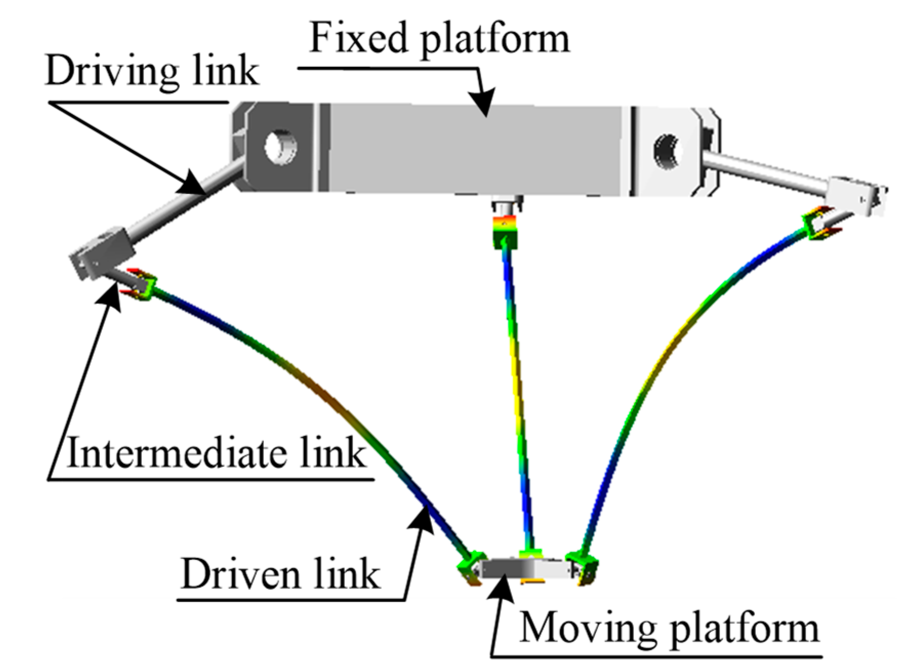
2. Flexible Spatial Parallel Robot

The flexible spatial parallel robot is a strongly coupled, time-varying, nonlinear multi-body system model. In this study, a spatial parallel robot with both flexible and rigid links in the kinematic branch chain was analyzed as an example, as shown in Figure 1.
The flexible spatial parallel robot is composed of a fixed platform, a moving platform, and three triangular symmetrical kinematic chains. The kinematic chain contains a total of three components: a driving link, an intermediate link, and a driven link. The driven link is a slender beam with a uniform circular cross section, and its length-to-diameter ratio is greater than 20. Therefore, the elastic deformation of the driven link during the movement of the system will affect the trajectory accuracy of the moving platform and the system stability. In addition, since the rotation axis of the driven link is perpendicular to the rotation axis of the driving link and the intermediate link, the driven link is a spatial flexible link in the global coordinate system. The constraint relationship of the flexible spatial parallel robot is shown in Table 1.

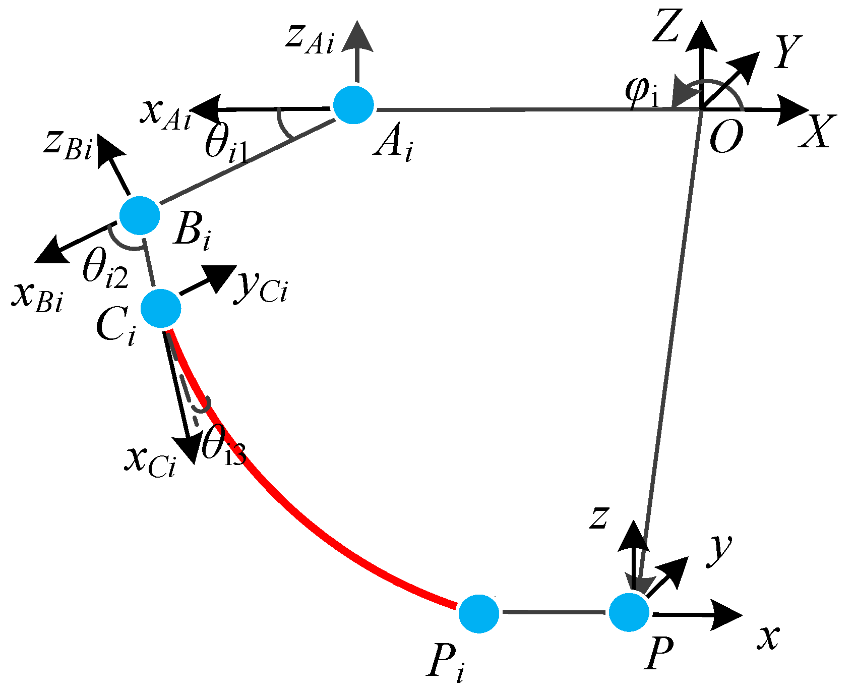
3. Dynamic Model of the Flexible Spatial Parallel Robot

3.1. Dynamic Model of the Flexible Spatial Link

Since the three kinematic chains are triangularly symmetric, after performing dynamic analysis on any one of the kinematic chains, the other two kinematic chains can be obtained through transformation relationships. The global coordinate system O-XYZ is set at the geometric center of the fixed platform, the local coordinate system is set at the joint of each component, and the angle between each component and its own rotation axis is θ i j , where i = 1 ,   2 ,   3 refers to the kinematic chain, and j = 1, 2, and 3 correspond to the driving link, intermediate link, and flexible spatial link, respectively. φi (i = 1, 2, 3) denotes the angle between the global coordinate system and the local coordinate system in the Z direction. The coordinate system P-xyz of the rigid moving platform is set at its geometric center. The system analysis model is shown in Figure 2.
To consider the impact of high-frequency vibrations on the system, the flexible spatial link can be divided into a series of discrete units by the finite element method, and then based on the boundary conditions, the deformation displacement of the flexible spatial link in the local coordinate system can be obtained as:
u f = N q f = [ u v w ] T
where N is the interpolation function matrix; q f is the generalized elastic coordinate in the local coordinate system; and u, v, and w represent the deformation displacements of the generalized elastic coordinates for any point of the flexible spatial link relative to the X-, Y-, and Z-axes of the local coordinate system, respectively.
The large-scale rigid motion of the system and the deformation motion of the flexible spatial links produce strong coupling effects, and the displacement field vector of any point w on a flexible spatial link considering the coupling effects can be established by the floating frame of reference method as:
r w = r 0 + T ( u 0 + u f )
where r 0 is the displacement vector of the origin of the floating frame of reference coordinate system in the global coordinate system, T is the transformation matrix, and u 0 is the undeformed vector of the flexible spatial link in the floating frame of reference coordinate system.
The absolute rotation angle of the flexible spatial link in the global coordinate system can be written as:
θ ˙ i 3 O = [ 0 θ ˙ i 1 + θ ˙ i 2 0 ] + T [ 0 0 θ ˙ i 3 + θ ˙ i 3 f ]
where θ ˙ i j is the rigid absolute angular velocity of the link, θ ˙ i 3 f is the elastic angle of the flexible spatial link, and θ ˙ i 3 O is the absolute angular velocity of the flexible spatial link in the global coordinate system. The deformation diagram of the flexible spatial link is shown in Figure 3.
Using the kinetic energy formula, the translational and rotational kinetic energy of the flexible spatial link can be calculated. At the same time, the elastic potential energy of the flexible spatial link can be directly calculated according to the deformation energy formula. The kinetic and potential energy formulas are as follows:
{ T 3 = 1 2 V ρ ( r ˙ w ) T r ˙ w d V + 1 2 0 l θ ˙ i 3 O d J f V 3 = 1 2 E 0 l [ a ( u ( x , t ) x ) 2 + I z ( 2 v ( x , t ) x 2 ) 2 + I y ( 2 w ( x , t ) x 2 ) 2 ] d x + 1 2 0 l G I p ( φ ( x , t ) x ) 2 d x
where l j and m j are the length and mass of the link, respectively; J 3 is the moment of inertia of the flexible spatial link; E is the elastic modulus; a is the cross-sectional area; Ip, Iy, and Iz are the moments of inertia of the flexible spatial beam cross-section along the x-, y-, and z-axes, respectively; u 0 , v 0 , and w 0 are the elastic displacement of any point on the flexible spatial link along the x-, y-, and z-axes, respectively; and φ 0 is the elastic angular displacement about the z-axis.

3.2. Dynamic Model of Rigid Links

Similarly, according to the kinetic energy formula, the kinetic and potential energy of the rigid driving link and the rigid intermediate link can be calculated as:
{ T 1 = 1 2 m 1 v 1 2 T 2 = 1 2 m 2 v 2 2 + 1 2 J 2 w 2 2 V 1 = 1 2 m 1 g l 1 V 2 = m 2 g l 1 sin ( θ i 1 ) 1 2 m 2 g l 2 sin ( θ i 1 + θ i 2 )
where m 1 and m 2 are the masses of the driving link and the intermediate link, respectively; l 1 and l 2 are the lengths of the driving link and intermediate link, respectively; v 1 and v 2 are the absolute angular velocities of the driving link and intermediate link, respectively; and J f represents the area moment of inertia of the intermediate link.

3.3. Dynamic Model of Flexible Spatial Parallel Robot

The kinetic energy and potential energy of the kinematic chain can be written as
{ T i = T 1 + T 2 + T 3 V i = V 1 + V 2 + V 3
where:
T 1 = 1 6 m 1 l 1 2 θ ˙ i 1 2 , T 2 = 1 2 m 2 l 1 2 θ ˙ i 1 2 + 1 6 m 2 l 2 2 θ ˙ i 1 2 + 1 2 m 2 l 1 l 2 θ ˙ i 1 θ ˙ i 2 cos ( θ i 2 ) , T 3 = 1 2 q ˙ T M q ˙ V 1 = 1 2 m 1 g l 1 sin ( θ i 1 ) , V 2 = 1 2 m 2 g l 2 sin ( θ i 1 + θ i 2 ) .
V 3 = 1 2 q T K q
where q and q ˙ represent the generalized position coordinates and the generalized velocity coordinates, respectively; and M and K represent the mass matrix and the stiffness matrix, respectively. The specific expression of M and K are shown in Appendix A.
Lagrange’s equations are typically used to derive the dynamics equations as follows:
d d t ( L q ˙ ) L q = Q
where L = T V , T is the kinetic energy, V is the potential energy, and Q is the generalized force.
By substituting Equation (6) into Lagrange’s equation, the dynamic equation of the kinematic chain can be derived.
Since the elastic deformation of the flexible link will cause a small displacement of the rigid moving platform and affect the control performance of the system, it is necessary to establish a dynamic equation of the moving platform considering the small displacement. Based on the coordination matrix [24] and boundary conditions, the actual displacement of the rigid moving platform in the global coordinate system can be written as:
P = P + J P Δ P
where J P = [ 1 0 0 0 P z P y 0 1 0 P z 0 P x 0 0 1 P y P x 0 ] is the coordination matrix, P = [ P x P y P z ] is the desired trajectory of the rigid moving platform, and Δ P is a small displacement. The kinetic and potential energies of the rigid moving platform can be written as:
{ T P = 1 2 ( P ˙ ) T m P P ˙ + 1 2 J w P T V P = m P g Z P
where m P , J, and w P T are the mass, moment of inertia, and absolute angular velocity vector of the rigid moving platform, respectively, and Z P is the displacement of the moving platform in the Z-direction in the global coordinate system. By substituting Equation (7) into Lagrange’s equation, the dynamics equation of the moving platform can be derived.
Assembling the dynamics equations of the kinematic chains and the moving platform, the dynamics equation of the flexible spatial parallel robot can be written as:
M q ¨ + K q + C q ˙ + G = τ
Since the inertia matrix of the flexible spatial link must be multiplied by the asymmetric transformation matrix to be expressed in the global coordinate system, the inertia matrix in the global coordinate system is also an asymmetric matrix. In the same way, the stiffness matrix will become a time-varying matrix after being transformed to the global coordinate system. C q ˙ is the vector containing the centrifugal and Coriolis forces, G is the generalized gravity vector of the system, and τ is the system-control torque.

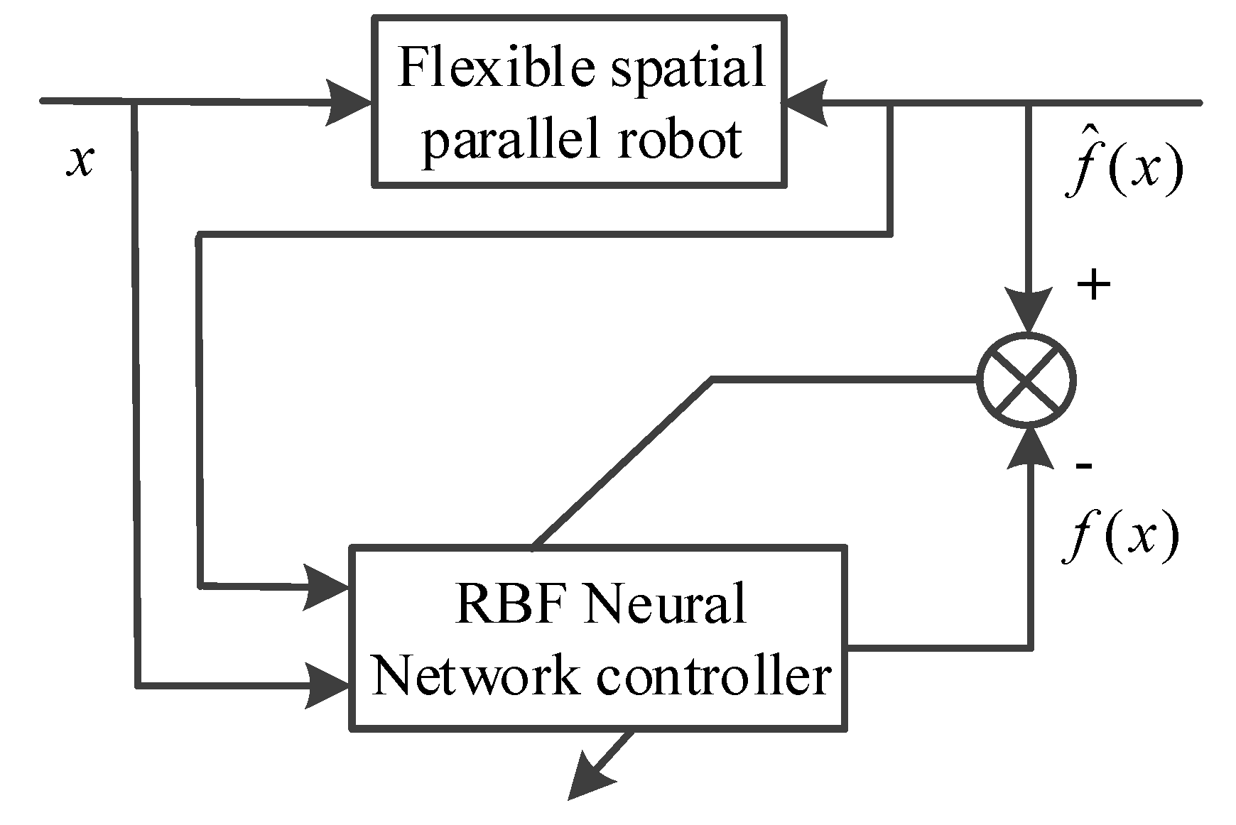
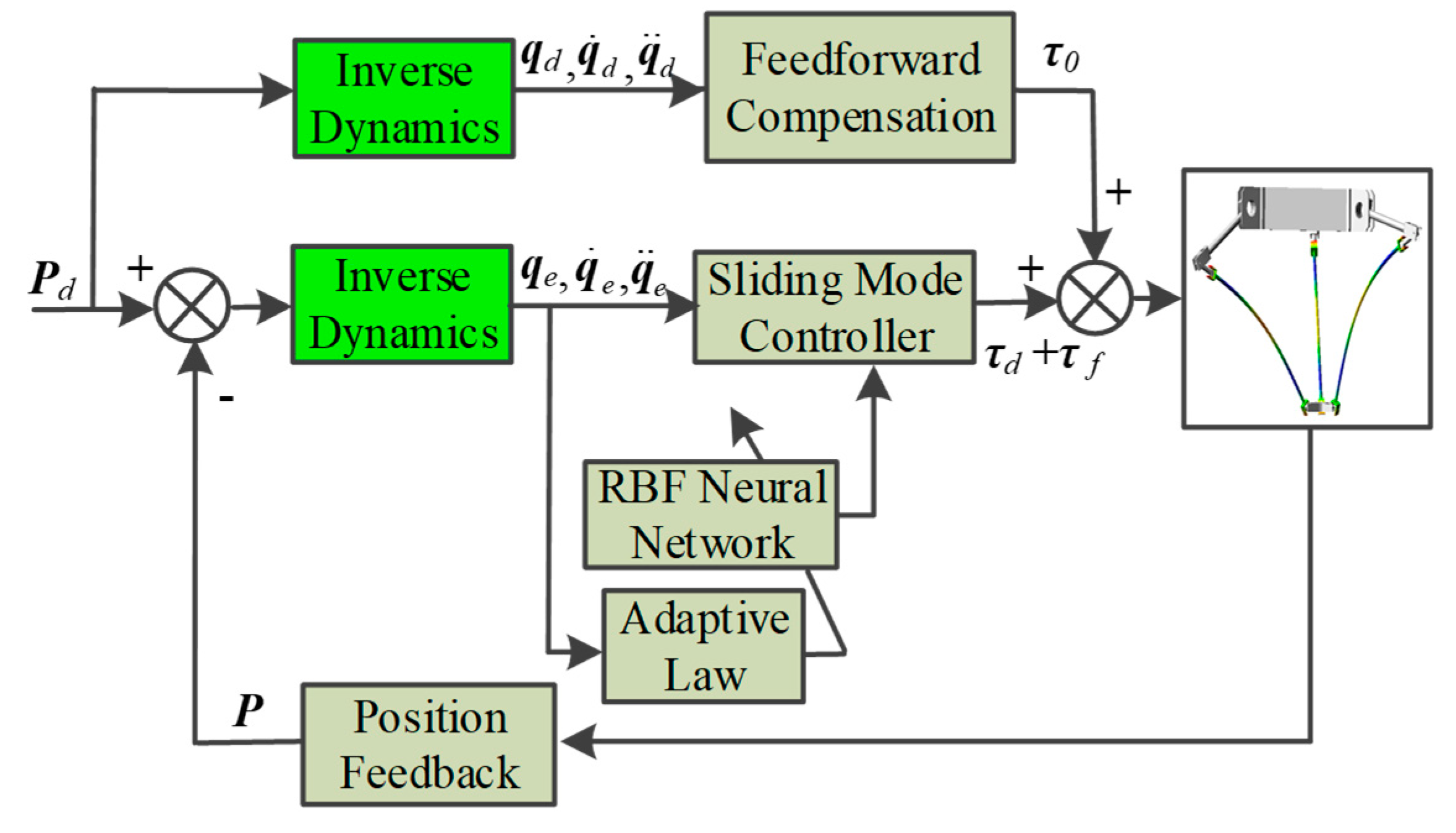
4. Intelligent Control

4.1. Problem Statement

The vibrations caused by the elastic deformation of the flexible spatial link are suppressed by active control, which improves the system’s ability to adapt to the external environment and suppresses the various modal responses. However, because the flexible spatial parallel robot is highly nonlinear, strongly coupled, and time varying, there will be certain errors in the control strategy based only on the dynamic model obtained by the nominal inertial parameters. In the actual work of the flexible spatial parallel robot, due to various external disturbances and its own model errors, it is difficult to obtain an accurate dynamic model, and the accuracy of the dynamic model will directly affect the design of the control strategy. The RBF (radical basis function) neural network is a type of feedforward neural network with excellent performance that can approximate arbitrary nonlinear functions with arbitrary precision, and has a global approximation capability. Compared with the BP (Back Propagation) neural network, the learning process of the RBF neural network converges faster, and there is no local minimum problem. In addition, the RBF neural network has strong nonlinear fitting ability, robustness, memory ability, and self-learning ability, which has a positive effect on the compensation of nonlinear systems. To improve the response speed and calculation efficiency and achieve high positioning accuracy, based on the precise dynamics model, the pre-calculated driving torque is subjected to feedforward compensation to ensure that the system has a fast response speed. At the same time, the sliding mode control algorithm is used to ensure that the system has good robustness. Making use of the excellent characteristics of a radial basis function (RBF) neural network, the unknown items of the system are nonlinearly approximated, and the entire network is optimized using a gradient descent algorithm to solve the problem of precise control and flexible suppression of flexible spatial parallel robots.

4.2. Feedforward Compensation

According to Equation (10), the control equation of the flexible spatial parallel robot can be obtained as:
M q ¨ + K q + C q ˙ + G = τ 0 + τ f + τ d
where τ 0 is the nominal model control torque, τ f is the model parameter error, and τ d is the uncertain external dynamic disturbance.
By substituting the ideal trajectory P into the dynamic equation (Equation (10)), the nominal model of the flexible spatial parallel robot can be obtained. The feedforward control compensates for the pre-calculated control torque. The feedforward compensation can be written as:
τ 0 = M 0 q ¨ + K 0 q + C 0 q ˙ + G 0
where M 0 , K 0 , C 0 , and G 0 represent the inertia matrix, stiffness matrix, centrifugal force matrix, and gravity matrix of the nominal model, respectively.

4.3. Sliding Mode Variable Structure Control

Equation (8) is rewritten as:
q ¨ = M Δ 1 ( τ f τ d K Δ q C Δ q ˙ G Δ )
where M Δ = M M 0 , K Δ = K K 0 , C Δ = C C 0 , and G Δ = G G 0 represent the inertia, stiffness, centrifugal force, and gravity matrices of the differences between the actual and nominal models, respectively.
Equation (10) is written as an equation of state, as follows:
{ x ˙ 1 = x 2 x ˙ 2 = f ( x ) + b u
where x 1 = q , x 2 = q ˙ , b = M Δ 1 , and f ( x ) = b ( K Δ x 1 C Δ x 2 G Δ ) .
The trajectory error can be written as:
{ e = x 1 x d e ˙ = x ˙ 1 x ˙ d e ¨ = x ¨ 1 x ¨ d = x ˙ 2 x ¨ d
where x ˙ d and x ¨ d are the desired angular velocity and angular acceleration of the drive link of the system, respectively. According to Equation (15), the system sliding mode function can be defined as
{ s = e ˙ + c e c > 0
The sliding mode reading law can be defined as:
s ˙ = K 1 s s K 2 s
where K 1 = d i a g ( k 11 , k 12 , , , k 1 m ) and K 2 = d i a g ( k 21 , k 22 , , , k 2 m ) are positive definite diagonal matrices, the reaching law can ensure the system state to reach the sliding surface quickly in finite time; therefore:
s ˙ = e ¨ + c e ˙ = x ˙ 2 x ¨ d = f ( x ) + b u x ¨ d + c e ˙
When s 0 , e and e ˙ also tend to zero. However, because the system vibration disturbance term is unknown and is affected by inertial parameters, the value of the f ( x ) is difficult to determine.

4.4. Adaptive Sliding Mode Neural Network Control

Considering that neural networks have universal approximation characteristics, an RBF neural network is used to approximate the system’s nonlinear uncertainty f ( x ) . The RBF neural network approximation model is shown in Figure 4.
As shown in Figure 4, the network input is x = [ x 1 x 2 x 3 ] T , and the ideal output of the RBF neural network can be written as:
h k = exp ( x c n k 2 b n k 2 )
f ( x ) = W T h ( x ) + ε
where h k = [ h 1 h k ] is the Gaussian function, k is the number of nodes in the hidden layer of the network, n is the number of inputs to the network, c n is the center vector, b n is the base width, and W and ε are the ideal neural network weights and approximation errors, respectively.
The actual output of the RBF neural network can be written as:
f ^ ( x ) = W ^ T h ( x )
where W ^ = [ w 1 w k ] is the estimate of the ideal neural network weight.
The adaptive law can be defined as:
W ^ ˙ = r s h ( x )
For an arbitrarily small ε , the RBF neural network has optimal weights W that satisfy the following equation:
ε = f ( x ) W T h ( x )
Equation (17) shows that the RBF neural network has the characteristics of approximating a nonlinear function with arbitrary precision.
The error index of the network approximation can be written as:
E ( t ) = 1 2 ( f ^ ( x ) f ( x ) ) 2
The weights are adjusted according to the gradient descent method, and:
{ Δ w k ( t ) = η E ( t ) w k = η ( f ^ ( x ) f ( x ) ) h k w k ( t ) = w k ( t 1 ) + Δ w k ( t ) + α [ w k ( t 1 ) w k ( t 2 ) ] ,
where η ( 0 ,   1 ) represents the learning rate, and α ( 0 , 1 ) represents the momentum factor. As long as the values of c n and b n are designed within the effective mapping range of the network input, the Gaussian function can be guaranteed to achieve an effective mapping.

4.5. Stability Analysis

The Lyapunov function is used to analyze the stability of the proposed control law in the flexible spatial parallel robot.
Taking the sliding mode function as Equation (16), the reaching law as Equation (17), and the model uncertainty τ d 0 and neural network adaptive law as Equation (22), the adaptive sliding mode neural network controller design of flexible spatial parallel robot can be written as:
{ τ = τ 0 + τ f + τ d τ 0 = M 0 q ¨ + K 0 q + C 0 q ˙ + G 0 τ f = M Δ ( K 1 s s + K 2 s ) τ d = W ^ T h
Therefore, the flexible spatial parallel robot system will be asymptotically stable to the desired trajectory.
The Lyapunov function is defined as:
V = 1 2 s T s + 1 2 t r ( W ˜ T r 1 W ˜ )
where W ˜ is the actual neural network weight.
Taking the derivative of both sides of Equation (27) yields the following:
V ˙ = s T s ˙ + t r ( W ˜ T r 1 W ˜ ˙ )
where W ˜ = W ^ W . Hence, W ˜ ˙ = W ^ ˙ = r h S T .
Therefore:
V ˙ = s T [ ( x ¨ d x ¨ ) + c e ˙ ] + t r ( W ˜ T r 1 W ˜ ˙ ) = s T [ x ¨ d + c e ˙ + M 1 K q + M 1 C q ˙ + M 1 G M 1 ( τ 0 + τ d + τ f ) ] + t r ( W ˜ T r 1 W ˜ ˙ )
The uncertainty term τ d of the model can be approximated by a neural network, so it can be expressed as follows:
τ d = W T h + ε
where ε is the neural network approximation error, and ε < ε N , the estimated value of the model uncertainty can be written as:
τ ^ d = W ^ T h
and therefore:
V ˙ = s T [ K 1 s s K 2 s + M 1 ( W T h + ε ) M 1 W ^ T h ] + t r ( W ˜ T r 1 W ˜ ˙ ) = s T [ K 1 s s K 2 s + M 1 ε ] + S T W ˜ T h + t r ( W ˜ T r 1 W ˜ ˙ ) c min K 1 s c min K 2 s 2 + s M 1 ε + S T W ˜ T h + t r ( W ˜ T r 1 W ˜ ˙ ) s [ c min K 1 M 1 ε ] c min K 2 s 2
The external interference and the approximation error of the neural network are bounded, and satisfy the following convergence conditions:
c min K 1 > ε M 1
Let η = c min K 1 ε M 1 + c min K 2 s , then η > 0 can be obtained. Thus, the first derivative of Lyapunov function can be written as:
V ˙ η s
Based on these equations, V ˙ 0 , and, according to the principle of LaSalle invariance, the state of the system can reach the sliding surface in finite time, and the system is progressively stable.
The control diagram is shown in Figure 5. P is the actual trajectory of the flexible parallel robot, and Pd is the ideal input of the system. The ideal input can be solved using the inverse dynamics to obtain the generalized position, generalized velocity, and generalized acceleration coordinates in the ideal state. Substituting them into the dynamic equation (Equation (10)) yields the driving torque τ 0 for the feedforward compensation, which allows the system to achieve a fast response speed. Because the system has modeling errors, vibrations are caused by flexible spatial link deformation and external interference, that is, unknown nonlinear items. The approximation characteristics of the RBF neural network were used in this study to approximate the unknown nonlinear items, and the sliding mode control algorithm ensures that the system has better robustness characteristics and high trajectory tracking accuracy.

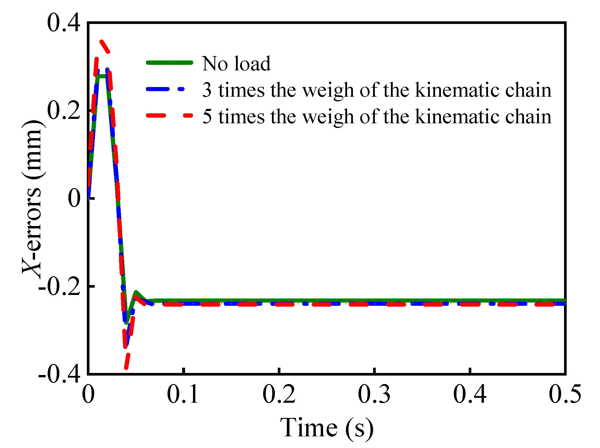
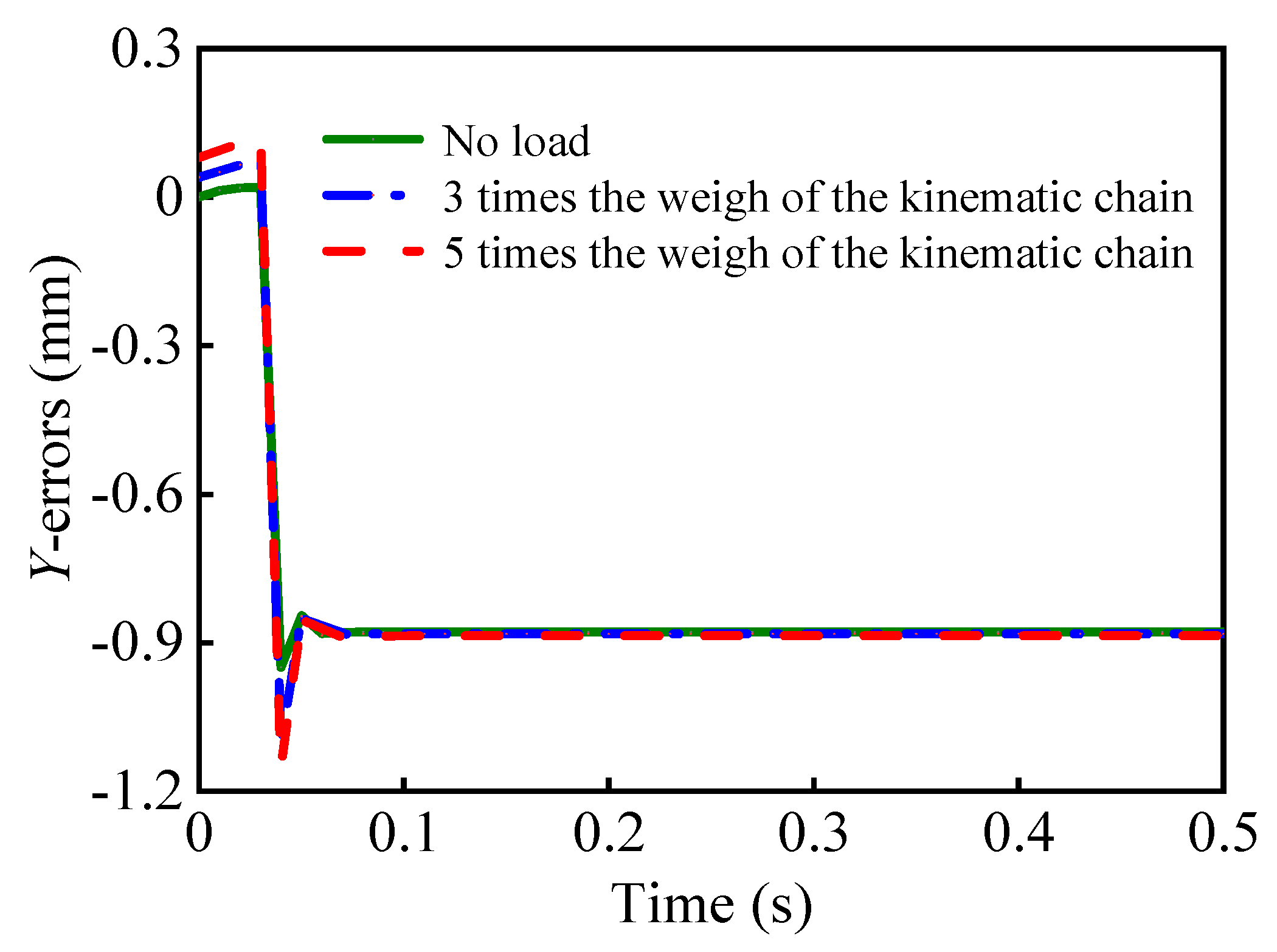
5. Simulation Results

To verify the correctness of the dynamic simulation model, the dynamic simulation model of the flexible spatial parallel robot was first compared with the results of a MATLAB numerical model, and the dynamic model was combined with a MATLAB/Simulink model to analyze the effectiveness of the control model. The inertial parameters of the flexible spatial parallel robot shown in Figure 1 are summarized in Table 2.
The comparison of the dynamic simulation model of the flexible spatial parallel robot and the MATLAB/Simulink numerical model is shown in Figure 6.

5.1. Dynamic Simulation Model

The dynamic simulation model was established using the ADAMS software. The specific modeling process was as follows.
(1)
Based on the SOLIDWORKS software, a three-dimensional model of the spatial parallel robot was constructed, and it was saved in (‘x_t’) format.
(2)
The three-dimensional model was imported into ADAMS, the constraint relationship between the components was set as shown in Table 1, and the material properties were defined as shown in Table 2. Since the flexible link was a simple homogeneous component, it was softened directly through the ADAMS/FLEX module, and the original rigid link was deleted. The constraints between the flexible link and its connected components were then reset.
(3)
An inverse dynamics analysis was performed on the dynamic simulation model by setting the moving platform drive.

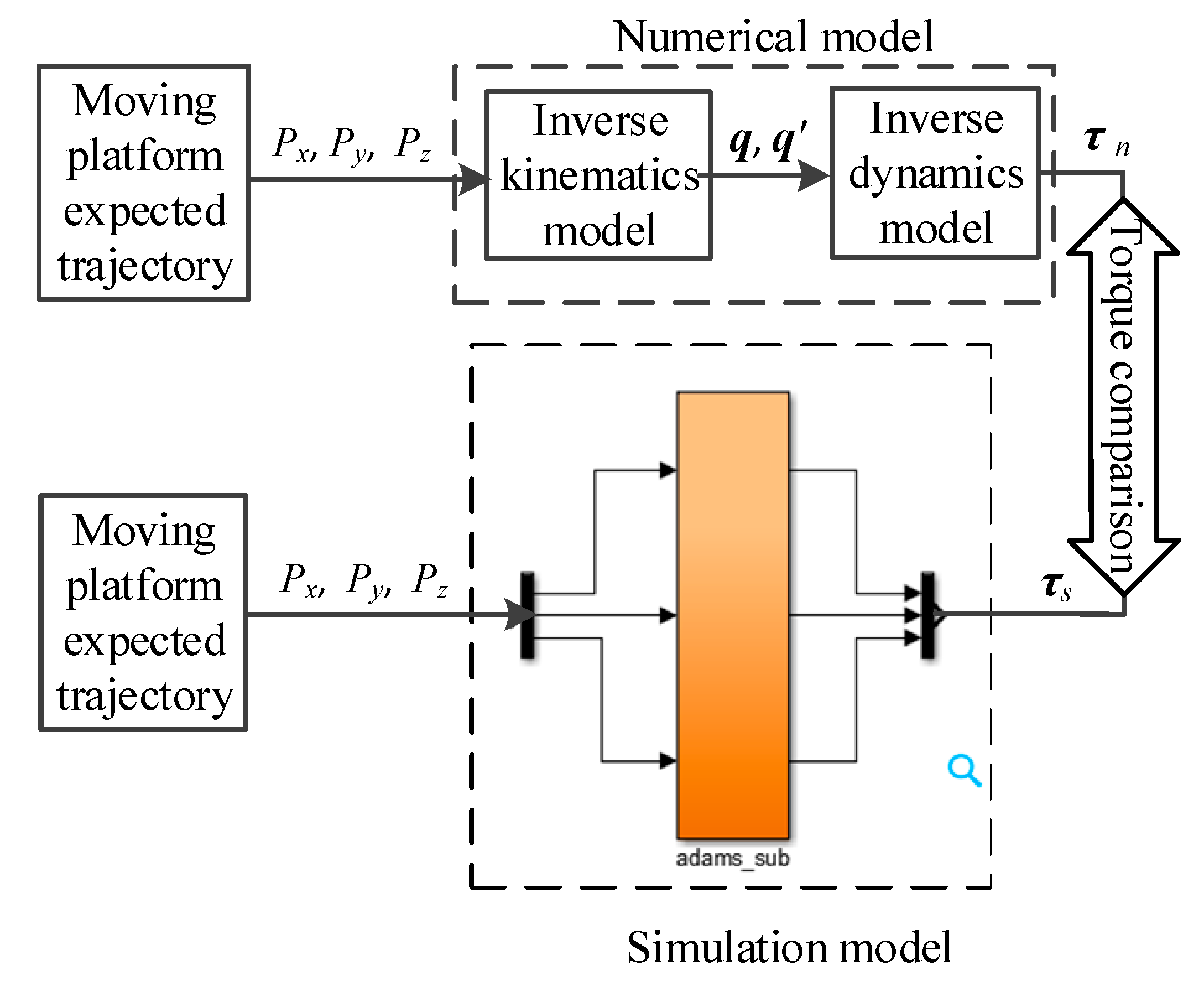
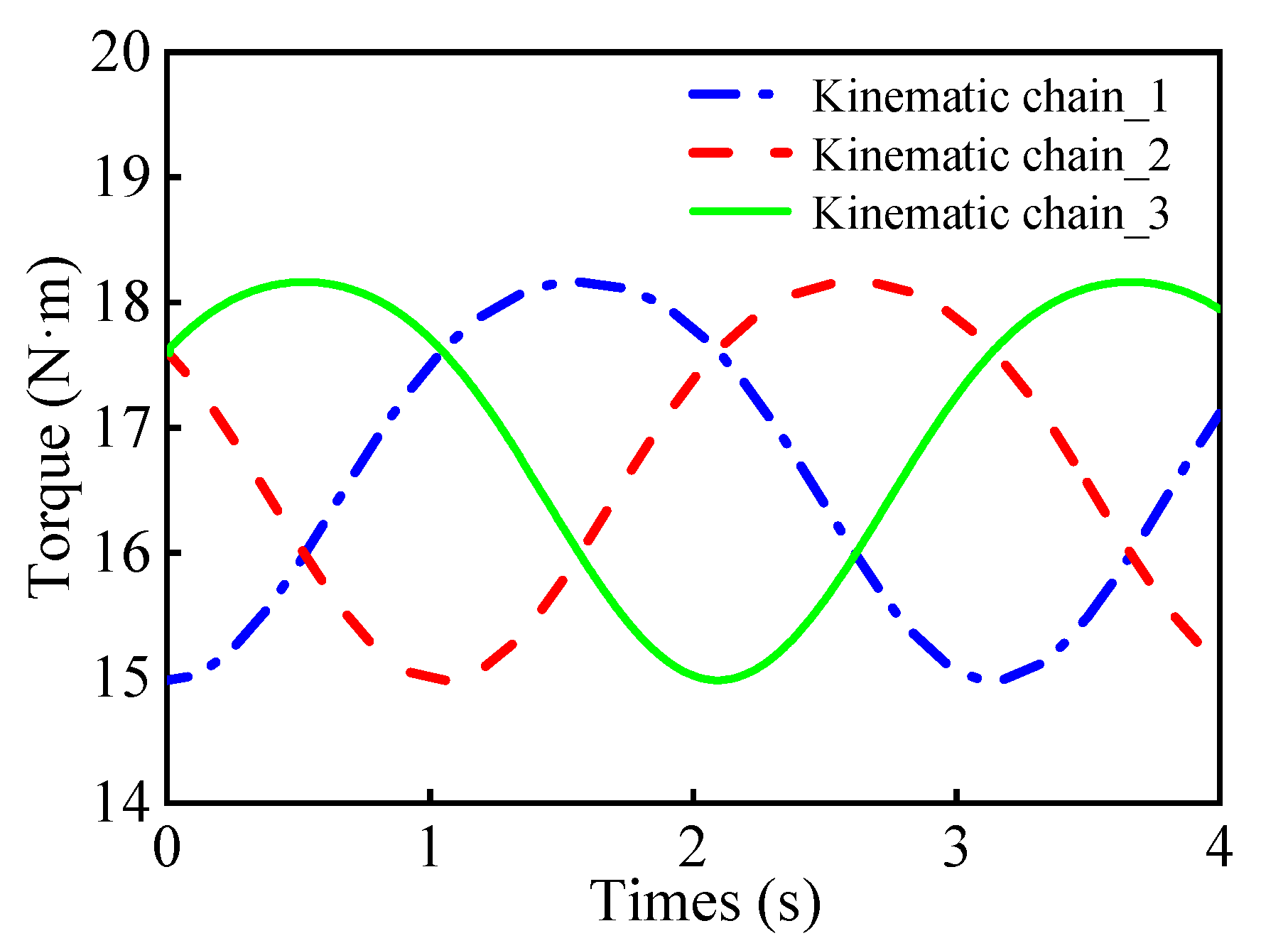
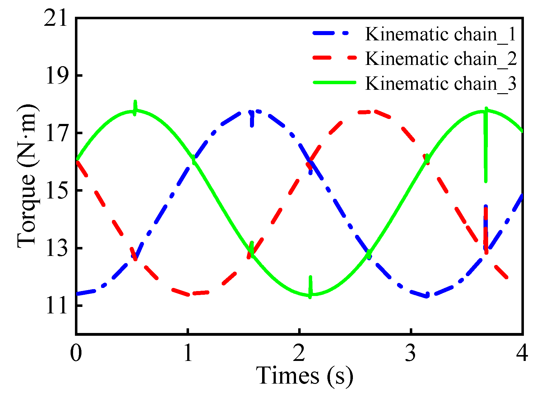
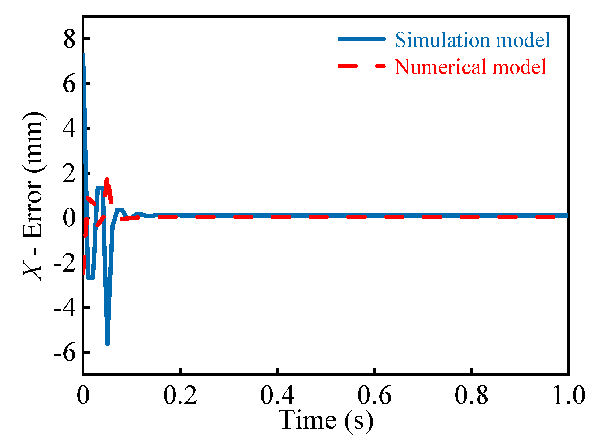
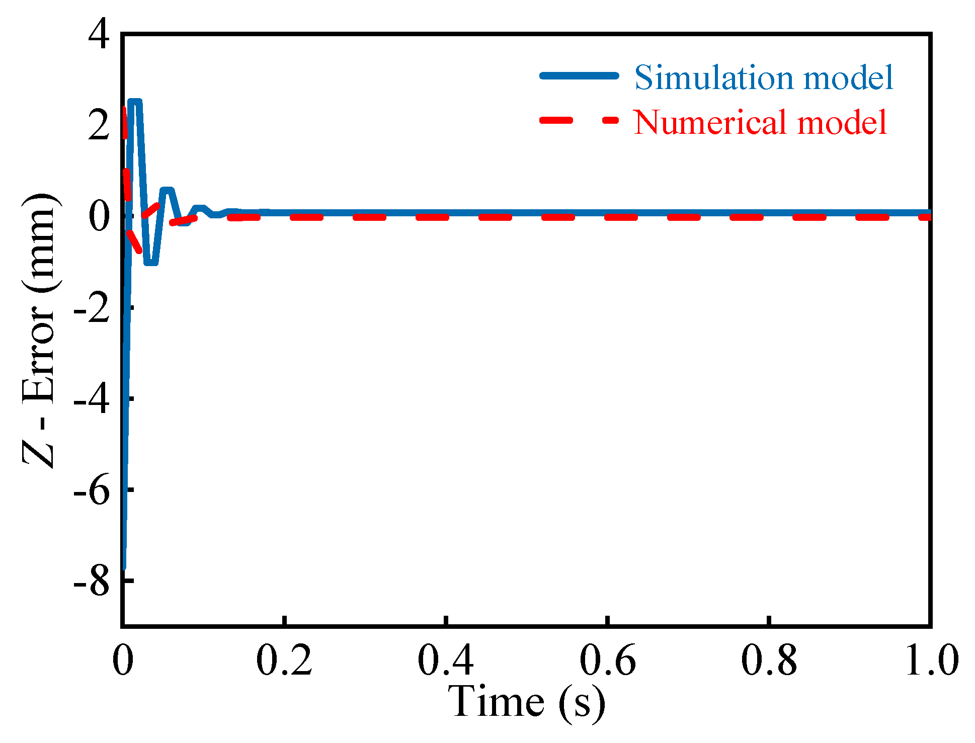
5.2. Numerical Model

According to the deduced dynamics equation (Equation (7)), the inverse kinematics model result of the numerical model was obtained by implementing it in MATLAB. The expected trajectory of the moving platform of the flexible spatial parallel robot is expressed as:
{ P x = 0.1 cos ( ω t ) P y = 0.1 sin ( ω t ) P z = 0.7
where the angular velocity ω = 2   rad / s . The flexible spatial parallel robot was then simulated based on the dynamics model. The inverse dynamics results could be obtained through simulation analysis, as shown in Figure 7 and Figure 8.
Based on the comparison of the dynamics results in Figure 6 and Figure 7, the motion trends of the kinematic chains of the flexible spatial parallel robot were consistent, but the dynamic simulation model was affected by assembly errors in the modeling process and the number of flexible links meshes, so the torque values were greater than those of the numerical model. This was consistent with the actual working conditions, and it proved the correctness of the established dynamic model. Furthermore, it provided a parameter reference for further control strategy research.

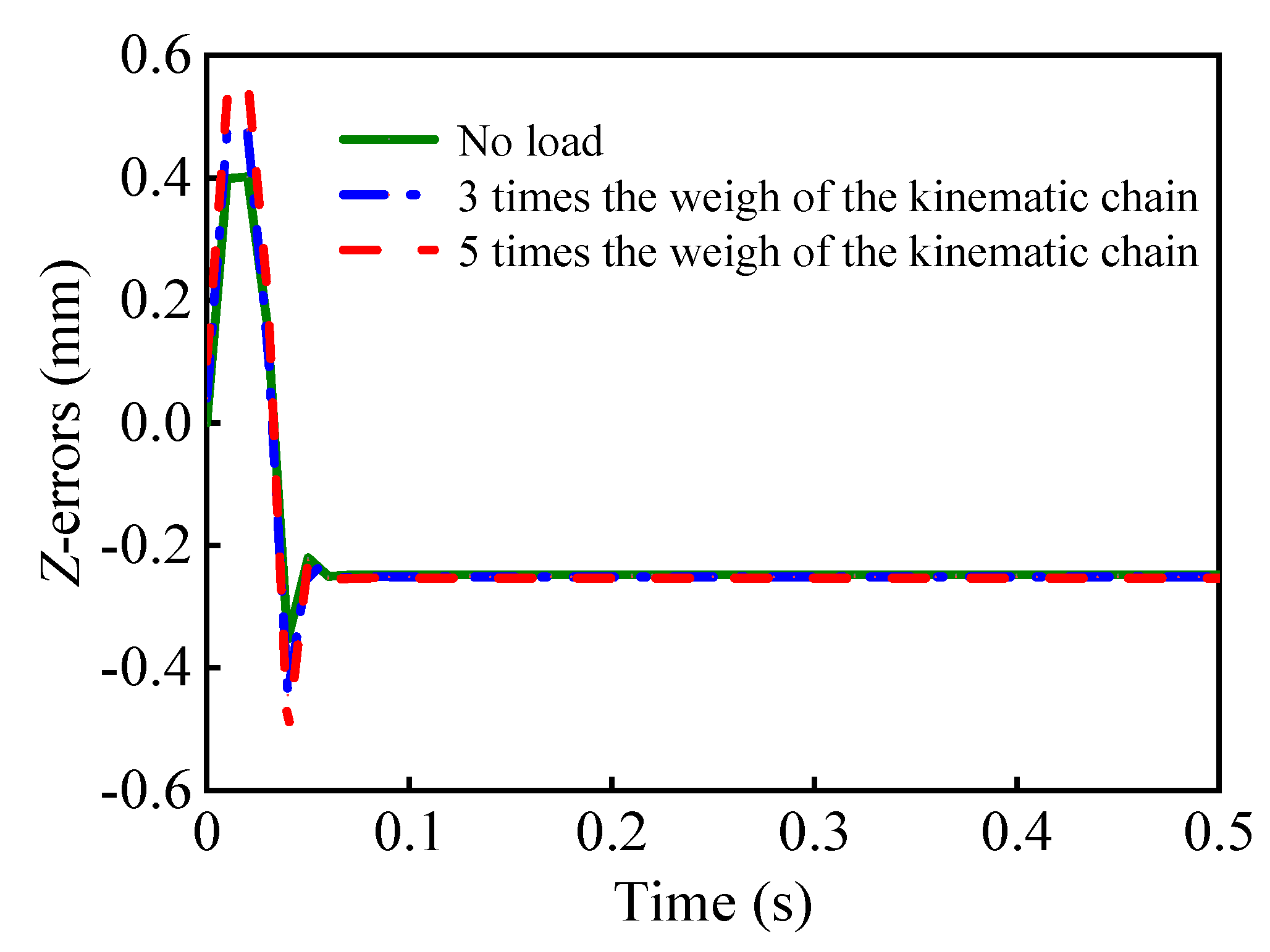
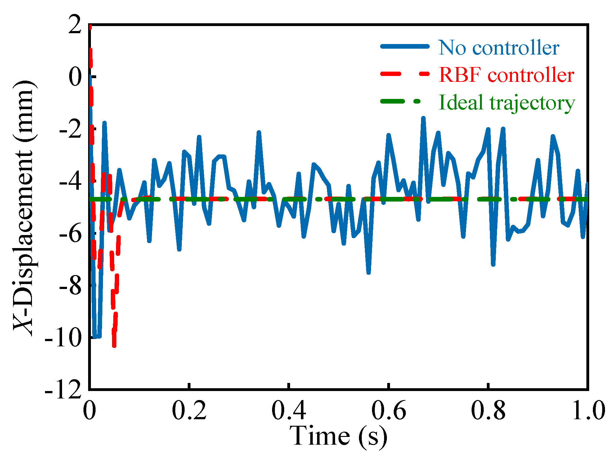
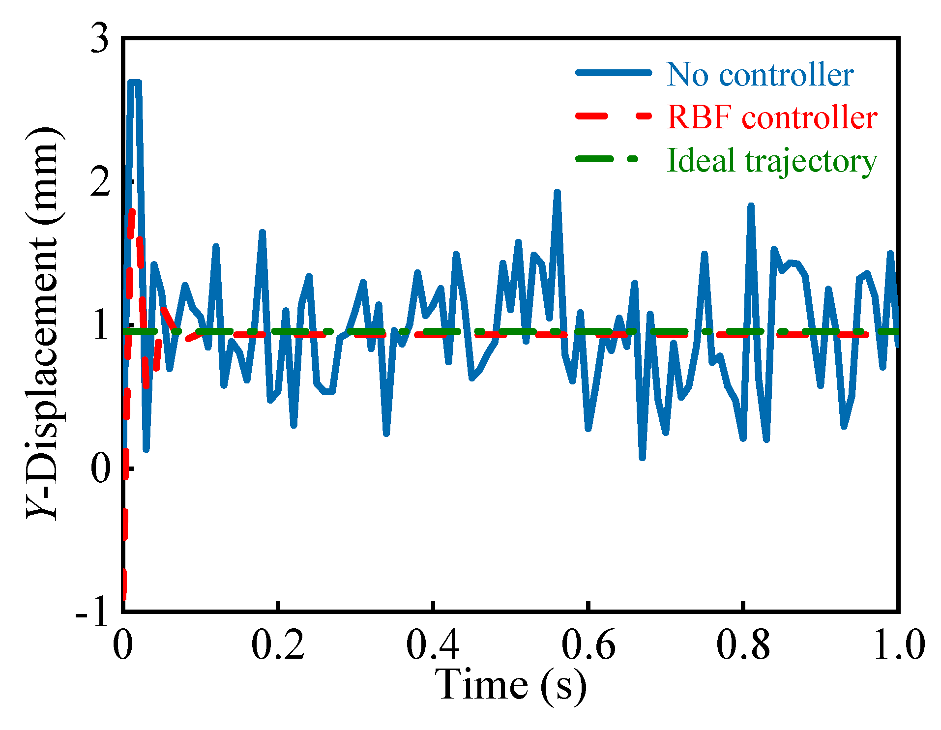
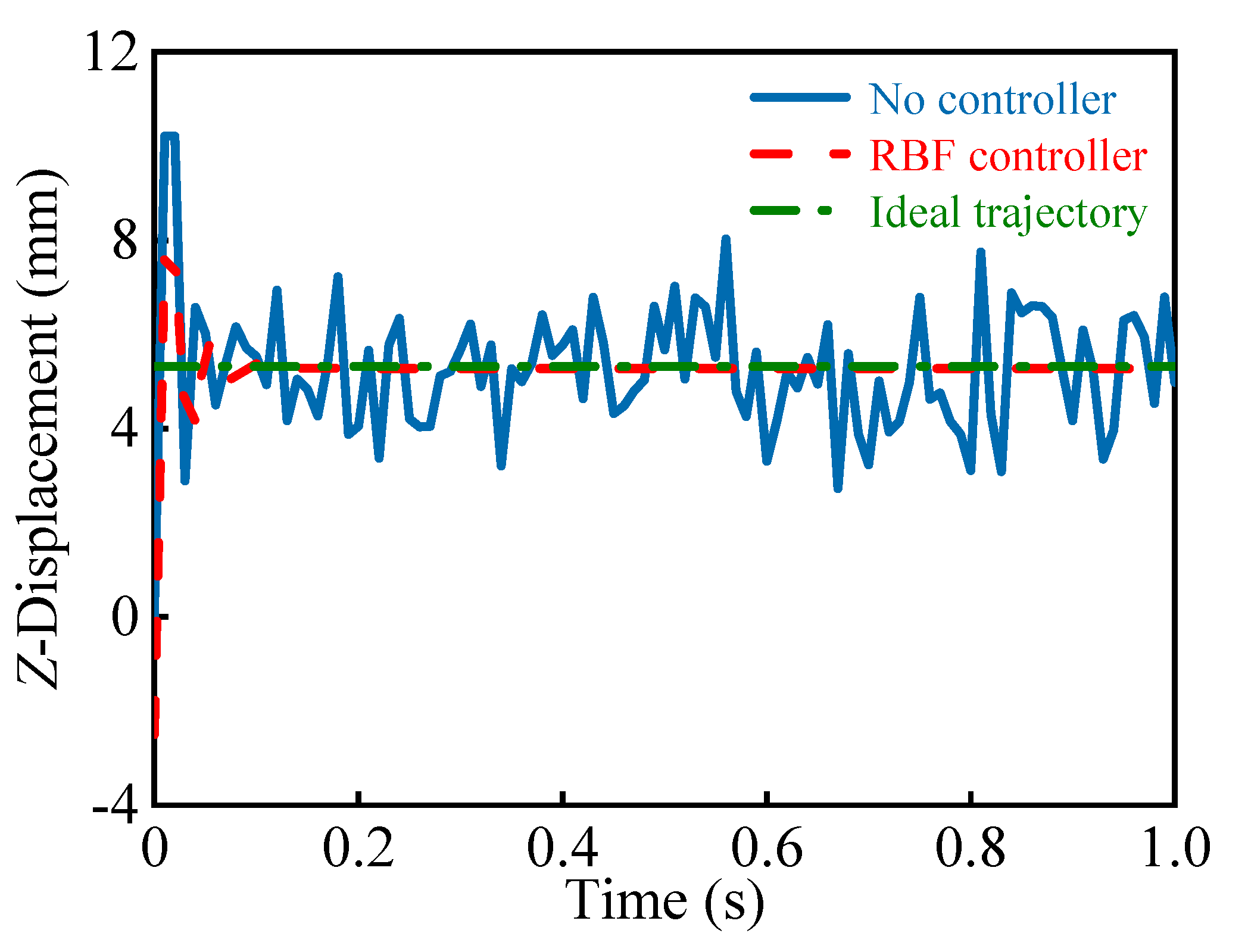
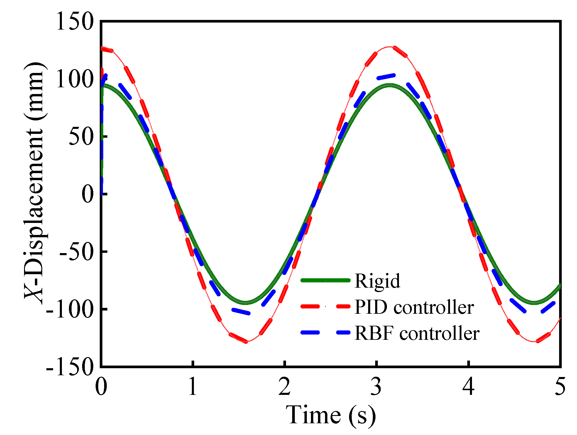
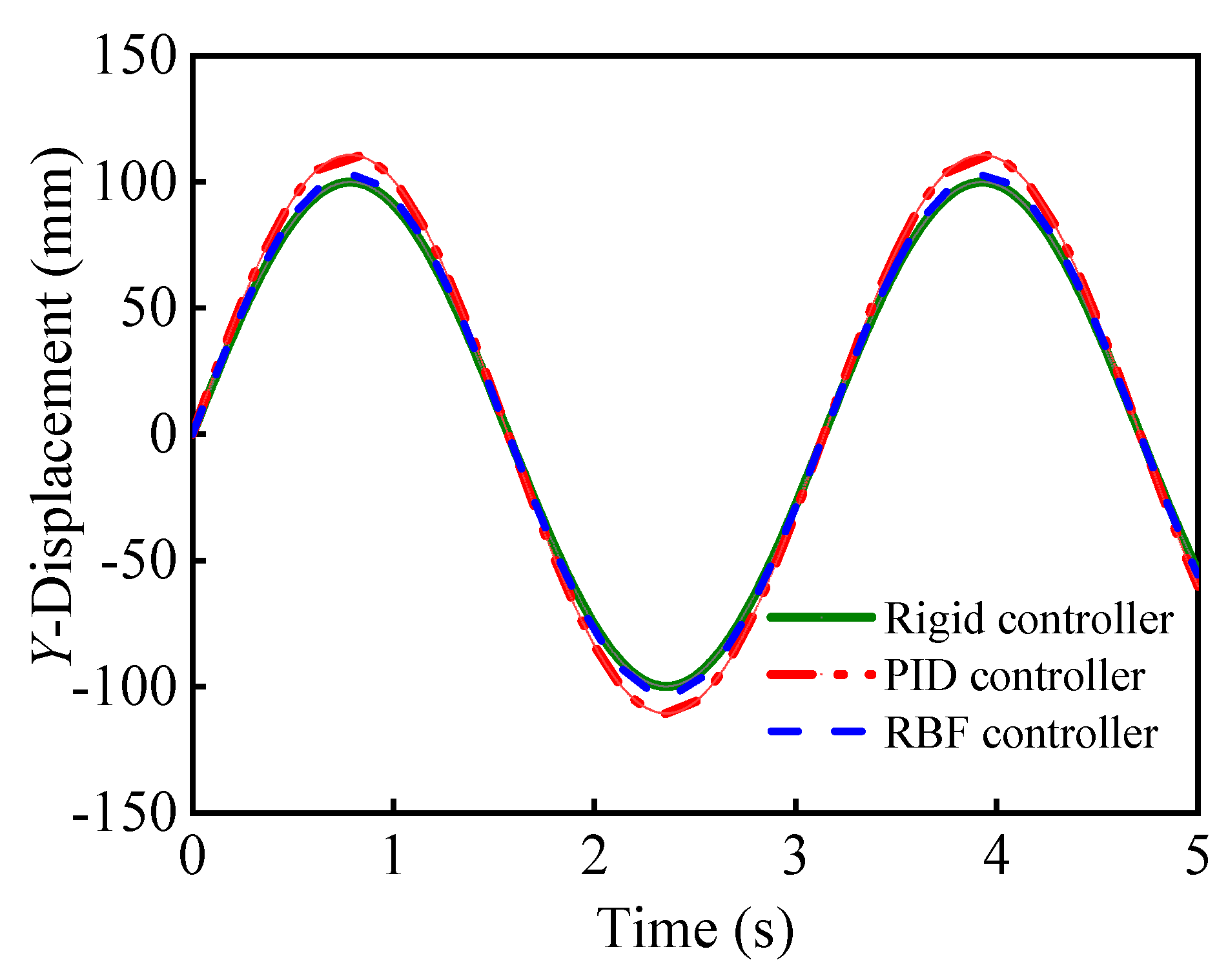
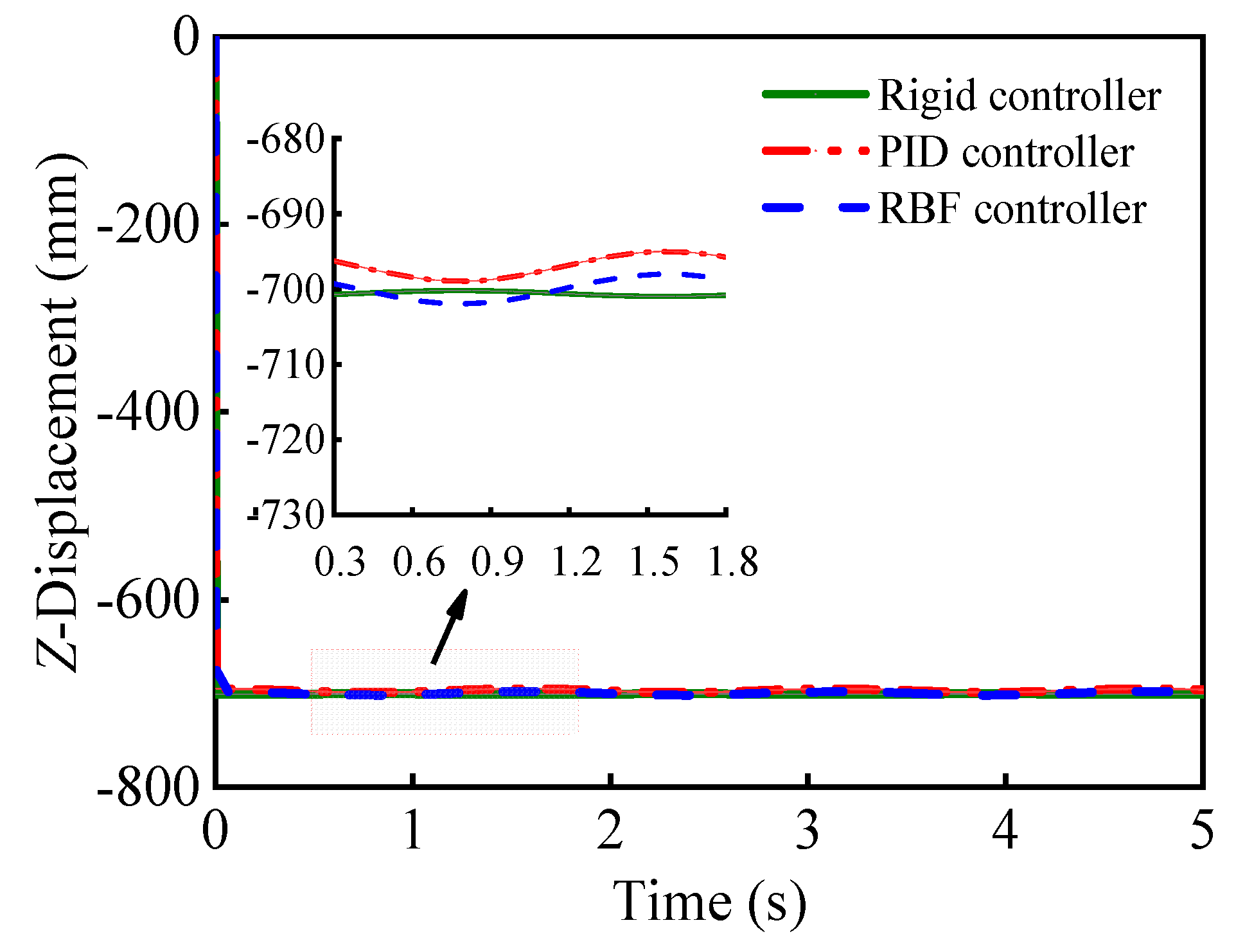
5.3. Control Simulation Results

Based on the established dynamic simulation model, the specific steps to establish a system control model through the combination of ADAMS and MATLAB/Simulink were as follows:
(1)
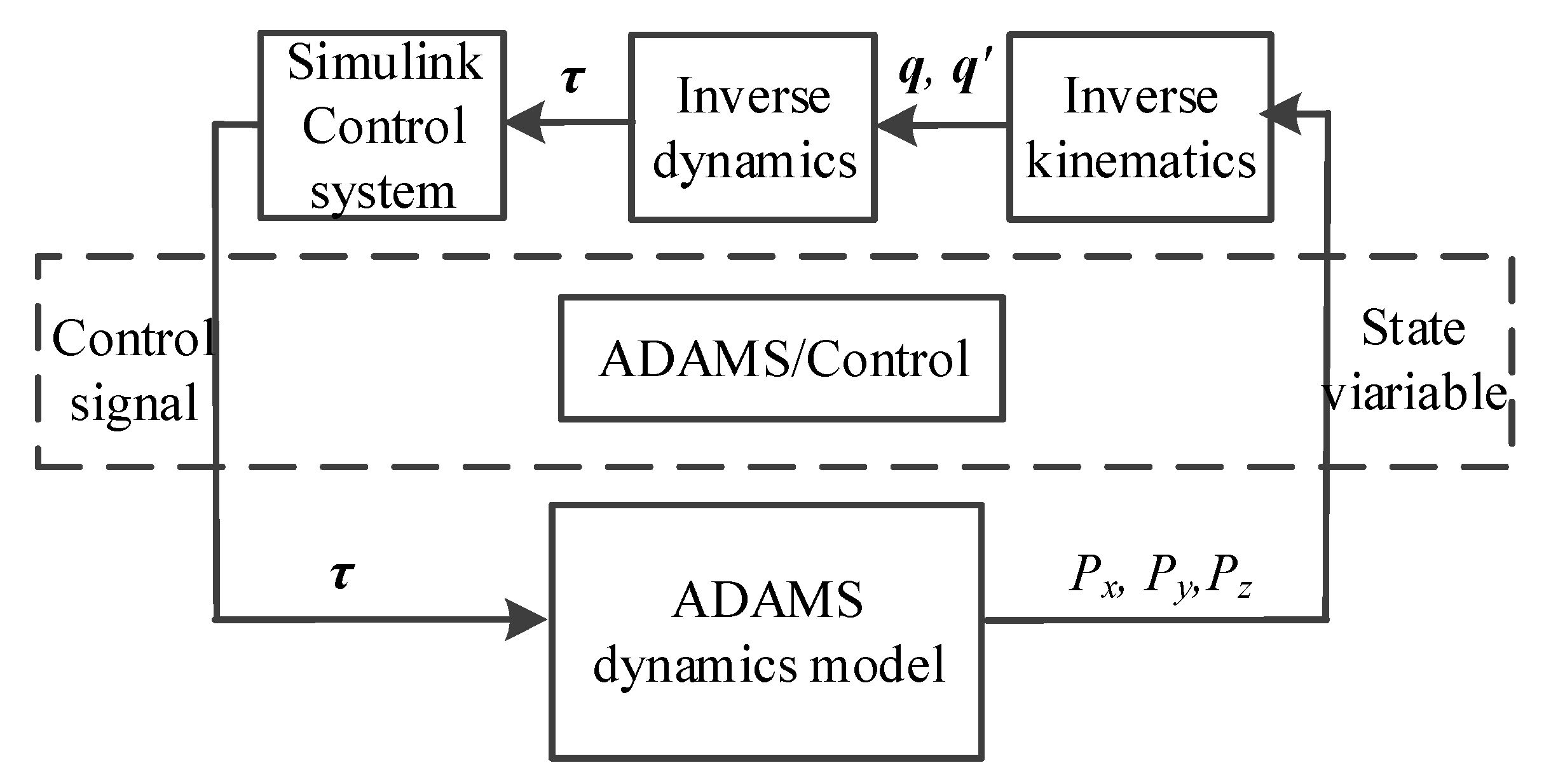
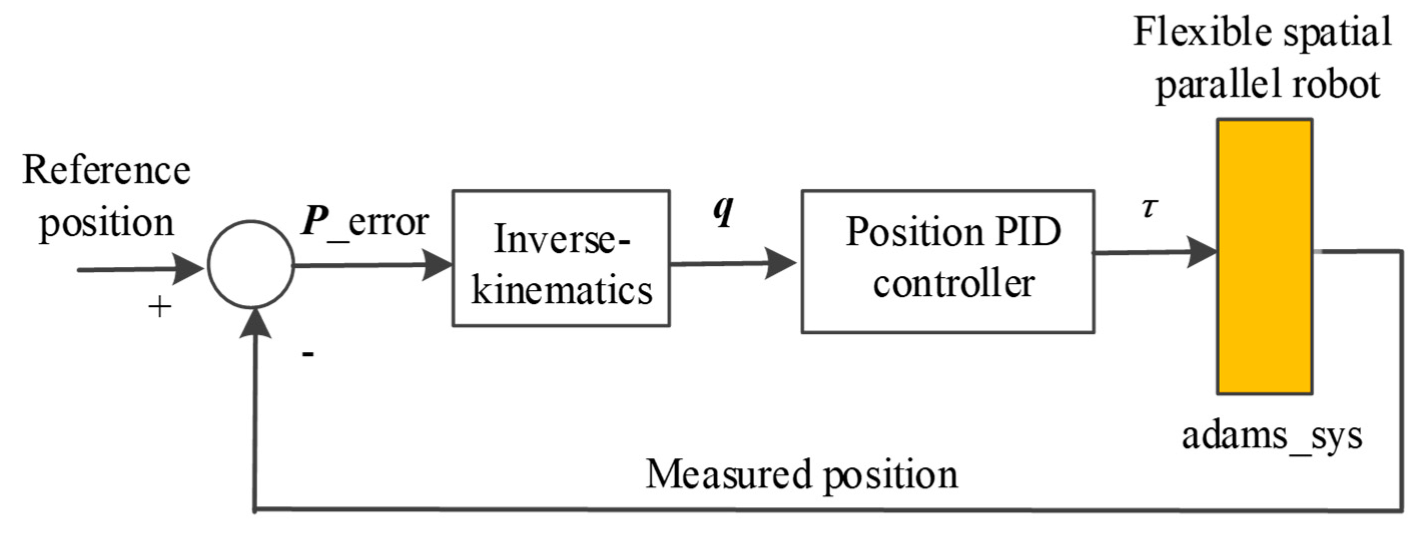
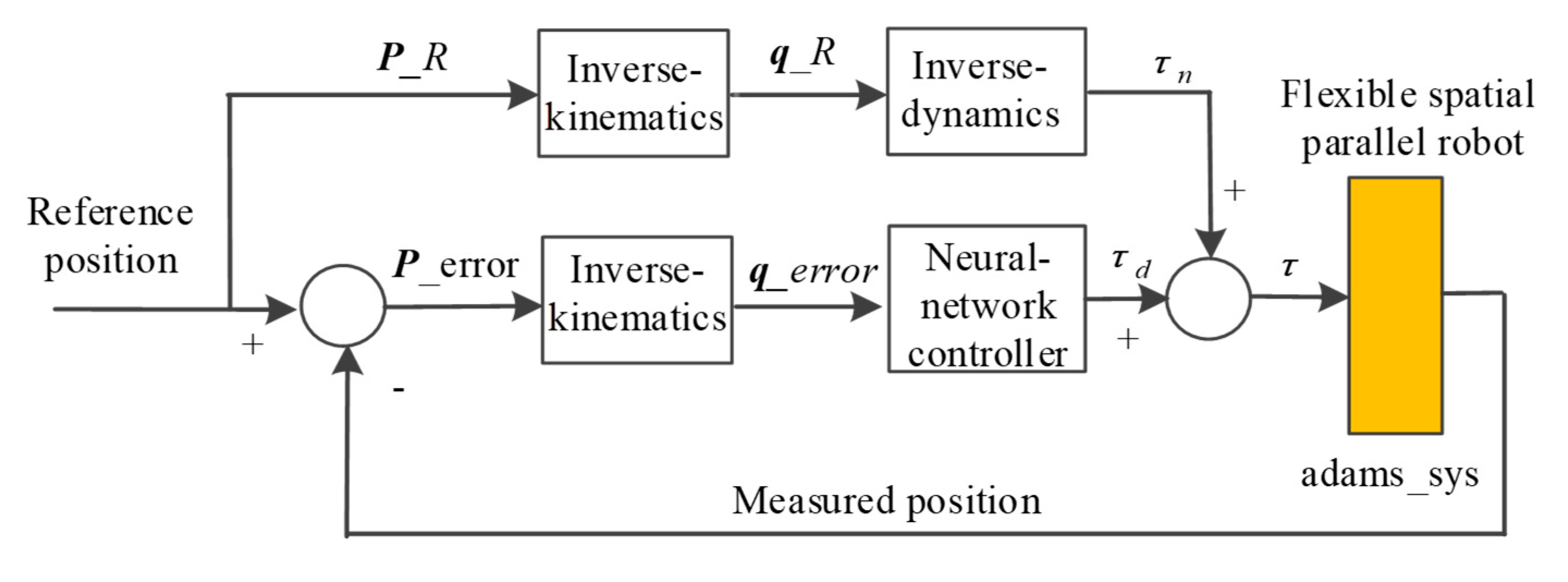
The output variable of the ADAMS model was the input variable of the MATLAB/Simulink control model. According to the control algorithm we proposed, the three driving torques of the kinematic chain were set as control input signals, and the actual trajectory of the rigid moving platform was the control output signal. The dynamic model and the control model were connected through the ADAMS/Control module.
(2)
MATLAB/Simulink were used to build the control system of the flexible spatial parallel robot. The information exchange diagram of the co-simulation control model is shown in Figure 9.
Based on the control algorithm we proposed, the control parameters can be written as input signal x = [ e e ˙ P d P ˙ d P ¨ d ] ; base width b n = 2 ; the network structure is taken as 5-n-1, where n is the number of hidden layer nodes. To analyze the influence of different network structures on the network approximation, n is set to 3, 5, 7, and 9, and the influence of the number of hidden layer nodes on the error accuracy and convergence speed is shown in Table 3.
It can be seen in Table 3 that as the number of hidden layer nodes increased, the error value first decreased, and then increased. When the number of hidden layer nodes was set to 5, the number of training steps was the smallest, the error convergence speed was the fastest, and the error value was the smallest. Therefore, the number of hidden layer nodes was set to 5.
To improve the control performance of the system, the RBF neural network was used to model multiple input and multiple output data through offline training. According to the derivation of the control strategy, the entire training sample error index was set according to Equation (22), and the gradient descent method was used to adjust the network weight, then the number of training samples was set to NS = 5000, and the error index change process was obtained after offline training as shown in Figure 10.
Using the trained network weights and Gaussian function parameters to test the data, the results are shown in Table 4.
It can be seen in Table 4 that the use of RBF neural network can well achieve recognition performance.
To verify that the proposed controller had finite time convergence, based on the control algorithm proposed in Equation (28), the convergence of the state trajectory of the numerical model and the simulation model were obtained through the state equation, and the results are shown in Figure 11, Figure 12 and Figure 13.
It can be seen in Figure 11, Figure 12 and Figure 13 that the trajectory trend of the simulation model and the numerical model was basically the same, and the trajectory error converged to 0 after a period of time. However, because the dynamic equation of the simulation model was solved directly by ADAMS, the solution accuracy of the model was affected by the modeling error, joint clearance, and mesh density, so that the convergence speed of the simulation model was faster than that of the numerical model, and the numerical floating range was larger than that of the numerical model. Among them, the error of the elastic displacement of the flexible spatial link of the simulation in the X direction was attenuated to 0 at 0.11 s from 5.2 mm at the initial 0.07 s; the error of the elastic displacement of the flexible spatial link of the simulation model in the Y direction was attenuated to 0 at 0.12 s from 0.8 mm at the initial 0.03 s; the error of the elastic displacement of the flexible spatial link of the simulation model in the Z direction was attenuated to 0 at 0.09 s from 2.3 mm at the initial 0.04 s. Therefore, the simulation model effectively realized the control simulation of flexible spatial parallel robot.
The comparison of the tracking accuracy of the moving platform in the X-, Y-, and Z-directions in a free state (zero load) and with loads of three and five times the total mass of the components are shown in Figure 14, Figure 15 and Figure 16.
As the load of the moving platform increased, the system vibration effect became more significant. The vibration was then suppressed under the action of the control algorithm and finally tended toward a stable value. Therefore, as long as the system control parameters were set reasonably, the moving platform could reach equilibrium, and the stability of the system movement was guaranteed.
The elastic deformation of the flexible spatial link was the main factor causing the system vibration. It is necessary to verify the effectiveness of the proposed control algorithm on the deformation of the flexible spatial link. Based on the simulation of the control algorithm, the trajectories of the flexible spatial link with or without the controller are shown in Figure 17, Figure 18 and Figure 19.
According to the trajectory comparison chart of the flexible spatial link, the trajectory vibrations of the system without control was greater than the trajectory vibration with control, which verified that the controller could effectively suppress the vibrations caused by the flexible deformation of the system.
To better highlight the superiority of the tracking performance of the control algorithm in this paper, under the same conditions, the position PID control algorithm was compared with the adaptive sliding mode neural network control algorithm. The control block diagram of the position PID and the adaptive sliding mode neural network are shown in Figure 20 and Figure 21.
The gain parameters of the position PID were K P = d i a g ( 100 150 100 ) , K I = d i a g ( 0.2 0.1 0.1 ) , and K D = d i a g ( 50 50 48 ) .
According to the control strategy shown in Figure 20 and Figure 21, the flexible spatial parallel robot was simulated based on the co-simulation control model, and the position tracking results of the geometric center of the rigid moving platform in the global coordinate system were obtained, as shown in Figure 22, Figure 23 and Figure 24.
Based on the same system parameters, the trajectory accuracy of the moving platform using the adaptive sliding mode neural network control algorithm was better than that under the position PID control algorithm, and the vibration phenomenon caused by elastic deformation was better suppressed. The flexible spatial parallel robot could effectively track the desired trajectory under the action of the controller, and realize synchronous movement. The tracking error gradually converged to 0, and no major fluctuations occurred when the system reached a stable state.
To observe the control effect of the different controllers more intuitively, the maximum deviations of tracking trajectories under different control methods were compared, and the results are shown in Table 5.
For the position PID control algorithm, the deviations of the rigid moving platform in the X-, Y-, and Z-directions were 3.372 mm, 2.072 mm, and 5.961 mm, respectively; while for the adaptive sliding mode neural network control algorithm, the deviations of the rigid moving platform in the X-, Y-, and Z-directions were 2.936 mm, 1.268 mm, and 2.96 mm, respectively. Compared with the PID control algorithm, the neural network control algorithm considered the dynamic performance of the system, approximated the system’s unknown nonlinear items, and suppressed the vibrations generated by the deformation of the flexible spatial link. The trajectory errors of the moving platform in the X-, Y-, and Z-directions were reduced by 12.1%, 38.8%, and 50.34%, respectively. Therefore, the adaptive sliding mode neural network control algorithm proposed in this paper not only had higher tracking accuracy, but also restrained the vibrations caused by the flexible deformation.

6. Conclusions

(1) In this paper, through a co-simulation of ADAMS and MATLAB/Simulink, a dynamic model and a control model of a flexible spatial parallel robot were numerically simulated. The correctness of the derived dynamic equations and the effectiveness of the control strategy were verified. The simulation results were basically consistent with the actual working conditions.
(2) Since the control algorithm proposed in this paper was designed based on an accurate dynamic model, it avoided the complicated parameter adjustment process and improved the accuracy of the control model.
(3) An adaptive sliding mode neural network control model was established for the system vibration phenomenon caused by the elastic deformation of the flexible spatial link in the flexible spatial parallel robot, and compared with the trajectory tracking accuracy of the position PID control algorithm. The control ability of the adaptive sliding mode neural network was superior, and the system stability and accuracy under its control were improved.

Author Contributions

Conceptualization, Q.Z., X.Z., L.L., T.D.; methodology, Q.Z., X.Z., L.L.; software, Q.Z., T.D.; validation, Q.Z., X.Z., L.L., T.D.; formal analysis, Q.Z.; investigation, Q.Z., X.Z., L.L., T.D.; resources, Q.Z., X.Z., L.L., T.D.; data curation, Q.Z., X.Z., L.L., T.D.; writing—original draft preparation, Q.Z., X.Z., L.L., T.D.; writing—review and editing, Q.Z.; visualization, Q.Z., X.Z., L.L., T.D.; supervision, Q.Z., X.Z., L.L., T.D.; funding acquisition, X.Z. All authors have read and agreed to the published version of the manuscript.

Funding

This research was partly supported by the National Key Research and Development Project (Grant No. 2017YFB1303502), Science and Technology Key Project of Tianjin Key Research and Development Program (Grant No. 20YFZCGX01050), Tianjin Municipal Education Commission Research Project (Grant No. 2017KJ259), Tianjin Research Program of Application Foundation and Advanced Technology (Grant Nos. 17JCYBJC18300 and 18JCYBJC87900), and Tianjin University of Technology Teaching Research Project (Grant No. ZD20-03).

Informed Consent Statement

Informed consent was obtained from all subjects involved in the study.

Acknowledgments

We thank LetPub (www.letpub.com) for its linguistic assistance and scientific consultation during the preparation of this manuscript.

Conflicts of Interest

The authors declared no potential conflicts of interest with respect to the research, authorship, and/or publication of this article.

Appendix A

K = [ E A L 0 0 0 0 0 E A L 0 0 0 0 0 12 E I z z L 3 0 0 0 6 E I z z L 2 0 12 E I z z L 3 0 0 0 6 E I z z L 2 12 E I y y L 3 0 6 E I y y L 2 0 0 0 12 E I y y L 3 0 6 E I y y L 2 0 G I P L 0 0 0 0 0 G I P L 0 0 4 E I y y L 0 0 0 6 E I y y L 2 0 2 E I y y L 0 4 E I z z L 0 6 E I z z L 2 0 0 0 2 E I z z L E A L 0 0 0 0 0 12 E I z z L 3 0 0 0 6 E I z z L 2 12 E I y y L 3 0 6 E I y y L 2 0 G I P L 0 0 4 E I y y L 0 S y m m e t r i c 4 E I z z L ] ;
M = [ 1 0 1 0 1 0 0 1 0 0 q m T ( d B θ 1 d t ) T q m T ( d B θ 2 d t ) T q m T ( d B θ n d t ) T B T ] m [ 1 0 1 0 1 0 0 1 0 0 ( d B θ 1 d t ) q m ( d B θ 2 d t ) q m ( d B θ n d t ) q m B ] ,
where B and m represent the transform matrix and mass matrix, respectively.

References

  1. Wang, Y.Q.; Lin, Q.; Wang, X.G.; Zhou, F.G.; Liu, J. Force/position hybrid control for a wire-driven parallel robot support system based on RBF neural network compensation. Control Decis. 2020, 35, 536–546. [Google Scholar]
  2. Pham, C.B.; Yeo, S.H.; Yang, G.; Kurbanhusen, M.S.; Chen, I.M. Force-closure workspace analysis of cable-driven parallel mechanisms. Mech. Mach. Theory 2006, 41, 53–69. [Google Scholar] [CrossRef]
  3. Liang, Y.; Liang, Q.; Wu, G.; Wu, W.; Sun, W.; Wang, Y. 3RPS/UPS parallel robot back-stepping control based on network observer. Eng. Comput. Appl. 2019, 55, 255–262. [Google Scholar]
  4. Shi, L.L.; Chen, Q. Backstepping sliding mode control for flexible-joint robotic manipulators based on neural network. Control Eng. China 2017, 24, 2268–2273. [Google Scholar]
  5. Chen, Q.; Tao, L.; Nan, Y.; Ren, X. Adaptive nonlinear sliding mode control of mechanical servo system with LuGre friction compensation. J. Dyn. Sys. Meas. Control 2015, 138, 021003. [Google Scholar] [CrossRef]
  6. Korayem, M.H.; Yousefzadeh, M.; Beyranvand, B. Dynamics and control of a 6-dof cable-driven parallel robot with visco-elastic cables in presence of measurement noise. J. Intell. Robot. Syst. 2017, 88, 73–95. [Google Scholar] [CrossRef]
  7. Zubizarreta, A.; Cabanes, I.; Marcos, M.; Pinto, C. Dynamic modeling of planar parallel robots considering passive joint sensor data. Robotica 2009, 28, 649–661. [Google Scholar] [CrossRef]
  8. Nevmerzhitskiy, M.N.; Notkin, B.S.; Vara, A.V.; Zmeu, K.V. Friction model of industrial robot joint with temperature correction by example of KUKA KR10. J. Robot. 2019, 2019, 1–11. [Google Scholar] [CrossRef]
  9. Talole, S.E.; Kolhe, J.P.; Phadke, S.B. Extended-state-observer-based control of flexible-joint system with experimental validation. IEEE Trans. Ind. Electron. 2010, 57, 1411–1419. [Google Scholar] [CrossRef]
  10. Tan, X.; Chen, G.; Sun, D.; Chen, Y. Dynamic analysis of planar mechanical systems with clearance joint based on LuGre friction model. J. Comput. Nonlinear Dyn. 2018, 13, 061003. [Google Scholar] [CrossRef]
  11. Shen, X.; Wang, B.; Yu, R.; Cui, X.H. Friction modeling and computed torque control of robot joints with adaptive RBF neural network compensation. J. China Univ. Metrol. 2020, 31, 71–78. [Google Scholar]
  12. Liu, S.Z.; Yu, Y.Q.; Du, Z.C.; Liu, Q.B. A summary of the dynamics analysis and control strategy of flexible manipulators. Ind. Instrum. Autom. 2008, 200, 18–24. [Google Scholar]
  13. Zhang, Q.; Zhang, X. Active residual vibration control of planar 3-RRR flexible parallel robots. Trans. Chin. Soc. Agric. Mach. 2013, 44, 232–237. [Google Scholar]
  14. Rahimi, H.N.; Nazemizadeh, M. Dynamic analysis and intelligent control techniques for flexible manipulators: A review. Adv. Robot. 2013, 28, 63–76. [Google Scholar] [CrossRef]
  15. Liang, J.; Chen, L.; Liang, P. The rigid-flexible coupling dynamics simulation and wavelet based fuzzy neural network control for space manipulator. Manned Spaceflight 2015, 21, 286–294. [Google Scholar]
  16. Yang, J.; Qiu, Z.; Zhang, X. Self-excited vibration control of a planar 3-RRR flexible parallel robot. J. Vib. Shock 2017, 36, 138–143. [Google Scholar]
  17. Zhang, Q.; Wang, R.; Zhou, L.; Tan, Z. Dynamic modeling and active vibration control of flexible parallel manipulator. J. Vib. Meas. Diag. 2013, 33, 1025–1031. [Google Scholar]
  18. Hu, J.; Zhang, X. Active vibration control and its simulation of a novel 2-DOF flexible parallel manipulator. China Mech. Eng. 2010, 21, 2017–2021. [Google Scholar]
  19. Zhang, X.; Mills, J.K.; Cleghorn, W.L. Multi-mode vibration control and position error analysis of parallel manipulator with multiple flexible links. Trans. Can. Soc. Mech. Eng. 2010, 34, 197–213. [Google Scholar] [CrossRef]
  20. Gan, D.; Dai, J.S.; Dias, J.; Seneviratne, L. Reconfigurability and unified kinematics modeling of a 3rTPS metamorphic parallel mechanism with perpendicular constraint screws. Robot. Comput. Integr. Manuf. 2013, 29, 121–128. [Google Scholar] [CrossRef]
  21. Zhang, X.; Wang, X.; Mills, J.K.; Cleghorn, W.L. Dynamic Modeling and Active Vibration Control of a 3-PRR Flexible Parallel Manipulator with PZT Transducers. In Proceedings of the 7th World Congress on Intelligent Control and Automation, Chongqing, China, 25–27 June 2008; pp. 461–466. [Google Scholar]
  22. Zhang, F.T.; Han, Y.F. Elastic vibration control for delta parallel robot. Mach. Design Manuf. 2016, 9, 166–172. [Google Scholar]
  23. Stefan, P.; Zbigniew, Z.; Adam, C. Basic aspects related to operation of engine catalytic converters. Int. J. Thermodyn. 2004, 7, 9–13. [Google Scholar]
  24. Huang, Z.; Kong, L.F.; Fang, Y.F. Mechanism Theory and Control of Parallel Robot; Machinery Industry Press: Beijing, China, 1997. [Google Scholar]
Figure 1. Schematic diagram of a flexible spatial parallel robot.
Electronics 10 00212 g001
Figure 2. The analysis model of the system.
Electronics 10 00212 g002
Figure 3. The deformation diagram for the flexible spatial link.
Electronics 10 00212 g003
Figure 4. The block diagram for the radial basis function (RBF) neural network approximation.
Electronics 10 00212 g004
Figure 5. The control block diagram.
Electronics 10 00212 g005
Figure 6. Comparison chart of the dynamics models.
Electronics 10 00212 g006
Figure 7. Dynamics results for the simulation model.
Electronics 10 00212 g007
Figure 8. Dynamics results for the numerical model.
Electronics 10 00212 g008
Figure 9. Data exchange diagram of the co-simulation control model.
Electronics 10 00212 g009
Figure 10. Change process of the error index.
Electronics 10 00212 g010
Figure 11. Tracking error of the flexible spatial link in X-direction.
Electronics 10 00212 g011
Figure 12. Tracking error of the flexible spatial link in Y-direction.
Electronics 10 00212 g012
Figure 13. Tracking error of the flexible spatial in Z-direction.
Electronics 10 00212 g013
Figure 14. Tracking accuracy of the moving platform in X-direction.
Electronics 10 00212 g014
Figure 15. Tracking accuracy of the moving platform in Y-direction.
Electronics 10 00212 g015
Figure 16. Tracking accuracy of the moving platform in Z-direction.
Electronics 10 00212 g016
Figure 17. Tracking curve of the flexible spatial link in X-direction.
Electronics 10 00212 g017
Figure 18. Tracking curve of the flexible spatial link in Y-direction.
Electronics 10 00212 g018
Figure 19. Tracking curve of the flexible spatial link in Z-direction.
Electronics 10 00212 g019
Figure 20. Control block diagram of position proportional–integral–derivative (PID) controller.
Electronics 10 00212 g020
Figure 21. Control block diagram of the adaptive sliding mode neural network controller.
Electronics 10 00212 g021
Figure 22. Tracking diagram of the displacement trajectory in X-direction of the rigid end effector.
Electronics 10 00212 g022
Figure 23. Tracking diagram of the displacement trajectory in Y-direction of the rigid end effector.
Electronics 10 00212 g023
Figure 24. Tracking diagram of the displacement trajectory in Z-direction of the rigid end effector.
Electronics 10 00212 g024
Table 1. The constraint relationship.
Kinematic PairComponent
Rotating pairDriving link, fixed platform
Rotating pairIntermediate link, driving link
Rotating pairDriven link, intermediate link
Hook hingeMoving platform, driven link
Table 2. The inertial parameters of the system.
ComponentDriving LinkIntermediate LinkDriven Link
Mass (kg)1.80.31.5
Length (m)0.40.10.8
Density (kg/m3)780178012740
Poisson’s ratio0.290.290.33
Elastic Modulus (N/m2)2.07 × 10112.07 × 10112.07 × 1011
Table 3. The analysis of the hidden layer nodes (mm).
Number of Hidden Layer NodesSteps to Reach the Target Number of TrainingError (mm)
343765.215
529472.016
735423.962
946084.372
Table 4. Test samples and results.
InputOutput
100010.9670.022−0.089
0.970.10001.0110.002−0.007
110.1010.9770.033−0.140
Table 5. Analysis of the deviation (mm).
DeviationControl AlgorithmXYZ
Maximum deviationRBF2.9361.2682.96
PID3.3722.0725.961
Note: RBF = radial basis function; PID = proportional–integral–derivative.
Publisher’s Note: MDPI stays neutral with regard to jurisdictional claims in published maps and institutional affiliations.

