Improving the Prediction Quality in Memory-Based Collaborative Filtering Using Categorical Features

Abstract

Despite years of evolution of recommender systems, improving prediction accuracy remains one of the core problems among researchers and industry. It is common to use side information to bolster the accuracy of recommender systems. In this work, we focus on using item categories, specifically movie genres, to improve the prediction accuracy as well as coverage, precision, and recall. We derive the user’s taste for an item using the ratings expressed. Similarly, using the collective ratings given to an item, we identify how much each item belongs to a certain genre. These two vectors are then combined to get a user-item-weight matrix. In contrast to the similarity-based weight matrix in memory-based collaborative filtering, we use user-item-weight to make predictions. The user-item-weights can be used to explain to users why certain items have been recommended. We evaluate our proposed method using three real-world datasets. The proposed model performs significantly better than the baseline methods. In addition, we use the user-item-weight matrix to alleviate the sparsity problem associated with correlation-based similarity. In addition to that, the proposed model has a better computational complexity for making predictions than the k-nearest neighbor (kNN) method.

1. Introduction

With the growth of information technology and the Internet, there is a seemingly never-ending flood of information on the web. However, searching for a specific item through a large amount of information is very challenging. Specifically, it is much more difficult to find items that best suit their needs and preferences when more choices are available. Recommender systems primarily emerged to solve this problem of information overload [1]. The task of the recommendation system is to connect information and users who are interested in it. It also helps users find information that is valuable to them. Thereby achieving a win-win situation for information consumers and information producers. For example, if you read suggested articles in a news aggregator app, you often find that it suits your taste. In fact, the recommendation engine computes your preferences based on your past behavior and then selects it from many news sources and pushes it to you.

Recommender systems have evolved dramatically over the last few decades. As a result, various algorithms and methods have been proposed to perform recommendations, including content-based methods (CB) and collaborative filtering methods (CF). These methods use different mechanisms to personalize the recommendations for different users in the system. However, the performance is not consistent across the range of application areas and different input types. Content-based recommenders require the rich content descriptions (e.g., metadata, descriptions, topics, etc.) of the items consumed by the user in the past [2]. For example, content-based e-commerce platform recommenders will generally rely on detailed information such as product category, description, prices, and producers. In contrast, collaborative filtering (CF) recommendation algorithms analyze a series of historical feedback (ratings) behaviors of users to find specific patterns to predict items to recommend [3,4]. The underlying assumption is that users who have similar tastes will rate the items similarly [5]. It is the most widely implemented technique in RS [1]. Many e-commerce companies, such as Amazon.com [6] and JD.com [7], rely on CF to offer their customers recommendations. In addition to these two specifics types, various other methods, including, but not limited to demographic-based, knowledge-based, communality-based, and utility-based, are often combined to form a hybrid recommender [1,8].

According to [3], the existing collaborative filtering recommendations algorithm can be further classified into two common classes: memory-based and model-based. The memory-based algorithm is essentially a heuristic algorithm that makes rating predictions based on the entire set of items the user previously rated. The ratings are predicted based on rating similarity between users. In contrast, the model-based algorithms [3,9] exploit ratings to learn a model. The learned model is then used to make predictions. Many machine-learning algorithms such as decision-tree [10], SVM [11], and naïve Bayes [12] are often used for this purpose. Despite the advancement of CF, several major problems [13] with CF remain unsolved. These include (1) data sparsity problem: Often, this problem happens when the items do not have enough users’ ratings. In most situations, the predictions’ accuracy is unsatisfactory since there are not enough ratings for making a good prediction [14]. (2) Cold-Start problem: it occurs when a new user joins the system. For the new user, the system does not have the prior ratings. Hence, it is difficult for the system to recommend any item. Similarly, new items also have the same problem. Since the item has not been rated by any user, it will not be recommended to anyone. Other recent approaches have employed user personality, mood recognition, and digital art analysis to improve recommendation effectiveness [15,16].

The success of online business transactions in e-commerce depends greatly on the effective design of the recommendation mechanism. Similar to the RSs, which use side information to boost prediction accuracy [17,18], this study proposes a recommender system that can generate personalized product recommendations based on category information. The metric is derived based on how much a user has liked a specific category and how much of a specific categorical feature belongs to an item. First, we obtain user-categories, how much the user likes the categories, using only the ratings. It is done by aggregating the user ratings given to all categories (ratings for all items) and normalizing the resulting categorical preference values. Similarly, the items-categories are calculated for each item using the user category values calculated from the previous step. The dot–product of these two feature vectors (user-categories and item-categories) results in a scaler weight value for a specific user-item pair. In contrast to the similarity matrix, the user-item-weight matrix is a rectangular matrix that ideally does not contain any empty entries. This taste matrix is then used to weight the predicted ratings. Inspired by the traditional kNN method, we proposed a novel method of choosing neighbors based on the users’ taste matrix. With the proposed method, we get surprisingly better improvements compared with other baseline methods. The specific contributions of this study are as follows:

• Propose a new weighting matrix that replaces a traditional similarity matrix in memory-based CF to increase the quality of the predictions;
• Alleviate sparsity in the weight matrix;
• Empirically prove the efficacy of the proposed model using three real-world datasets;
• Proposed a novel approach for explainability in recommender.

Accordingly, our experimental results show that the proposed model outperforms other benchmark methods in recommendation accuracy. We also tested the proposed method with three additional metrics, namely precision, recall, and coverage, to evaluate the recommendation quality. Our method significantly outperforms all the baselines, including traditional kNN-based methods, and has a similar performance as the state-of-the-art methods. The proposed framework can also be effectively applied to any online e-commerce system, helping sellers promote their products and services, only using customer ratings and item features.

The rest of the article is arranged as follows: In the next section, we formalize the proposed model. In Section 3, we present the results of the experiments conducted to evaluate the model. Before the conclusion, we discuss the implications and limitations of the model. We conclude the article by briefly discussing the overview of the study and future work.

2. Proposed Model

2.1. Preliminaries (Problem Statement)

Let ${\mathrm{r}}_{u,i},{\mathrm{r}}_{v,i}\in R_{\left|U\right|\times \left|I\right|}$ be the ratings of users $u,v\in U$ for item $i\in I$ in the rating matrix $R_{\left|U\right|\times \left|I\right|}$. Given the user’s rating history, the goal is to predict ratings for the items that the user has not yet rated. This is often done by taking $k$ neighbors similar to the target user and weighting their rating with the similarity between two users. The basic k-nearest neighbor (kNN) formula shown below will be used as our baseline algorithm.

$$\widehat{r_{u,\dot{i}}}=\frac{{{\displaystyle \sum }}_{v\in N_i^k\left(u\right)}Si{m}_{u,v}\times r_{v,i}}{{{\displaystyle \sum }}_{v\in N_i^k\left(u\right)}Si{m}_{u,v}}$$

(1)

In this equation, $\widehat{r_{u,\dot{i}}}$ is the prediction to of item $i$ for user $u$, $N_i^k\left(u\right)$ is the set of $k$ neighbors of user $u$ that have rated the item $i$, $r_{v,i}$ is the rating given to item $i$ by the neighbor $v$ and $Si{m}_{u,v}$ is the similarity between user $u$ and user $v$. The similarity between $u$ and $v$ is calculated using Pearson’s correlation, which is given by:

$$Si{m}_{u,v}=\frac{{{\displaystyle \sum }}_{i\in I_u\cap I_v}\left(r_{u,i}-\overline{r_{u,\dot{i}}}\right)\left(r_{v,\mathrm{i}}-\overline{r_{v,\dot{i}}}\right)}{\sqrt{{{\displaystyle \sum }}_{i\in I_u\cap I_v}{\left(r_{u,i}-\overline{r_{u,\dot{i}}}\right)}^2{{\displaystyle \sum }}_{i\in I_u\cap I_v}{\left(r_{v,\mathrm{i}}-\overline{r_{v,\dot{i}}}\right)}^2}}$$

(2)

In Equation (2), based on the correlation of user $u$, $v$’s commonly rated items, we can get the similarity between two users.

2.2. Model

In memory-based methods CF, the similarity between users (or items) serves as a weight matrix, which is just one of the most important factors that affect the accuracy of the prediction. Many possible other factors could be used to improve prediction accuracy or even enhance the system’s performance.

The proposed method uses explicit and implicit categorical features such as genre to find a user’s preference for a specific item. First, we use the user’s rating and categories of the item to calculate the user-categories. The collective user-categories of all users who have rated a specific item is then used to find actual categories of the item (item-categories). In movie datasets, this vector defines how much a specific movie (item) belongs to a genre (category). The user-categories vector is then combined with the item-categories vector to find the user-item-weight score, which measures how much a user likes a specific movie. The idea is that if the user has a higher preference for a certain category (please note that we categorize movies by genre. Thus, the keyword category and genre are used interchangeably). The movie has a higher score for that category; the predicted rating will be higher. The method is described below.

Let$G=\left\{g_1,g_2,\cdots ,g_k,\cdots ,g_m\right\}$ be set of all categories of the items in the data set. Item $i\in I$ can be represented in terms of a vector of categories $\overrightarrow{g_{\dot{i}}}$ as in the following equation.

$$\overrightarrow{g_{\dot{i}}}=\left\{g_{i1},g_{i2},\dots ,g_{ik},\dots ,g_{im}\right\}$$

(3)

Since all movies are labeled with one or more genres by the producers, a movie always has at least one category (i.e., $\left|g_{ik}=1\right|>0$). For all the items $i\in I_u$ rated by the user $u$ and if the category $g_{ik}=1$, then $g_{ik}=r_{u\left(i\right)}$, composing a new vector ${\overrightarrow{g}}_i^{*}$ from $\overrightarrow{g_{\dot{i}}}$. The user-categories vector of user $u$ can be calculated as follows:

$$\overrightarrow{s_u}=\frac{{{\displaystyle \sum }}_{i\in I_u}\overrightarrow{g_{\dot{i}}^{*}}}{{{\displaystyle ||\sum }}_{i\in I_u}{\overrightarrow{g_{\dot{i}}^{*}}{\displaystyle ||}}_1}$$

(4)

where $\overrightarrow{s_u}$ indicates the user-categories of the user $u$ and denominator is the sum of total ratings in $\overrightarrow{g_{\dot{i}}^{*}}$. The denominator can also be interpreted as the total collective ratings given to all genres by user $u$. Please note that this value is always greater than or equal to the user $u$’s total rating. The value of each entry in the resulting vector $\overrightarrow{s_u}$ represents the user $u$’s degree of preference for the respective genre. One of the metric’s advantages is that it defines the user’s preference for a specific genre as a continuous value rather than a discrete value.

As mentioned earlier, movies are classified by producers or experts. However, this classification does not consider the viewers’ opinions. Initially, we represented it as a binary vector $\overrightarrow{g_{\dot{i}}}$ in Equation (4). Since collaborative filtering uses other users’ views while making predictions, it is intuitive that the movie recommendation using genre information would increase the prediction accuracy. It is also intuitive to consider all user’s ratings (i.e., user’s preference) to estimate the movies’ actual genres, rather than simply relying on producers or experts. We use the user-categories vector $\overrightarrow{s_u}$ in Equation (5) to calculate new genre values $\overrightarrow{c_{\dot{i}}}$ for movies as follows:

$$\overrightarrow{c_{\dot{i}}}=\frac{{{\displaystyle \sum }}_{u\in U_i}\overrightarrow{s_u} \times r_{u,i}}{{{\displaystyle \Vert \sum }}_{u\in U_i}\overrightarrow{s_u} \times r_{u,i}{{\displaystyle \Vert }}_1}$$

(5)

where $r_{u,\mathrm{i}}$ is the user $u$’s rating for item $i$. Similar to the elements of $\overrightarrow{s_u}$, elements of $\overrightarrow{c_{\dot{i}}}$ are normalized and range between zero and one. The final user-item-weight score is calculated by taking the dot product of both the user’s taste $\overrightarrow{s_u}$ and $\overrightarrow{c_i}$ as follows:

$$w_{u,i}=\overrightarrow{s_u} ⨂\overrightarrow{ c_{\dot{i}}}$$

(6)

where $w_{u,i}$ is user-item-weight.

The prediction $\widehat{r_{u,\mathrm{i}}}$ is made by mean rating $\overline{r_u}$ of the target user $u$ adding to the bias part as follows:

$$\widehat{r_{u,i}}=\frac{{{\displaystyle \sum }}_{j\in N_k\left(u\right)}{w}_{u,j}\times r_{u,j}}{{{\displaystyle \sum }}_{j\in N_k\left(u\right)}{w}_{u,\mathrm{j}}},$$

(7)

Please note that instead of using $k$ similar users as the nearest neighbors, we use the k highest user-item-weight value in this user’s rating history. We assume these selected items are the items this user knows best, so we can use these items’ rating to make the prediction for the item $i$. It is common in real-world scenarios to find users with no neighbors due to the high item-to-user ratio. In these special cases, where users have no neighbor (when the user rate very few items), a common practice is to assign the mean rating to the prediction. This would result in all predictions for the target user be the same. However, in our method, since the user-item-weight score $w_{u,j}$ for each user-item pair is unique in Equation (7), the prediction will be different for each item.

2.3. Algorithm

The generate_weight method in Algorithm 1 outlines the steps involved in the generation of the weight matrix. As seen in lines 2 and 3, we first initialize $\overrightarrow{s_u}$ and $\overrightarrow{c_{\dot{i}}}$ with 19 zeros (an entry for each genre). We loop through all the items to find their genres, from lines 8–12 and in line 13 $\overrightarrow{s_u}$ is then normalized. For $\overrightarrow{s_u}$, as shown in line 9, we can get each user’s rated items and $\overrightarrow{g_{\dot{i}}}$ of this item by Equation (3). The rating is then used to replace the element with a value of 1 in the array to get $\overrightarrow{g_{\dot{i}}^{*}}$ as shown in line 10. The $\overrightarrow{s_u}$ is then used to calculate new genre weight $\overrightarrow{c_{\dot{i}}}$ for the item $i$ (lines 16–25). For $\overrightarrow{c_{\dot{i}}}$, as shown in line 21, we first get the users of this item, check these users’ taste, and multiply each entry by the rating, as shown in line 21. Therefore, as shown in line 26, the user-item-weight score $w_{u,i}$ can be derived by the dot product of $\overrightarrow{s_u}$ and $\overrightarrow{c_{\dot{i}}}$. Once the user-item-weight score is generated, we can make the predictions by Equation (7).

Algorithm 1. Pseudocode for calculating the user-item-weight score ($w_{u,i}$) algorithm.
1:	procedure Generate_Weight $\left(RatingMatrix\right)$
2:	$\overrightarrow{s_u}=\left[0, 0, 0, 0, 0, 0, 0, 0, 0, 0, 0, 0, 0, 0, 0, 0, 0, 0, 0\right]$
3:	$\overrightarrow{c_i}=\left[0, 0, 0, 0, 0, 0, 0, 0, 0, 0, 0, 0, 0, 0, 0, 0, 0, 0, 0\right]$
4:	$n\_users=length\left(RatingMatrix.row\right)$
5:	for $i=0, i++, i<n\_users$ do
6:	$u = RatingMatrix.row\left(i\right)$
7:	$n\_items = length\left(u\right)$
8:	for $j=0, j++ , j<n\_items$ do
9:	$\overrightarrow{g_{\dot{i}}}=getItemCate\left(u\left[j\right]\right)$
10:	$\overrightarrow{g_{\dot{i}}^{*}}=addRatings\left(\overrightarrow{g_{\dot{i}}}, RatingMatrix\left[i\right]\left[j\right]\right)$
11:	$\overrightarrow{s_u} +=g_i^{*}$
12:	end for
13:	$\overrightarrow{s_u}=\overrightarrow{s_u} / sum\left(\overrightarrow{s_u}\right)$
14:	end for
15:	$n\_items = length\left(RatingMatrix.coloum\right)$
16:	for $i=0, i++, i<n\_items$ do
17:	$item = RatingMatrix.coloum\left[i\right]$
18:	$n\_users = length\left(item\right)$
19:	for $j=0, j++, j<n\_users$ do
20:	$s_{item\left[j\right]}= getUserTaste\left(item\left[j\right]\right)$
21:	$\overrightarrow{c}=s_{item\left[j\right]} \times RatingMatrix\left[item\right]\left[item\left[j\right]\right]$
22:	$\overrightarrow{c_{\dot{i} }}+=\overrightarrow{c}$
23:	end for
24:	$\overrightarrow{c_{\dot{i}}}=\overrightarrow{c_{\dot{i}}} / sum\left( \overrightarrow{c_{\dot{i}}}\right)$
25:	end for
26:	$w_{u,i}=\overrightarrow{s_u}⨂\overrightarrow{ c_{\dot{i}}}$
27:	return $w_{u,i}$
28:	end procedure

2.4. A Toy Example

Consider the following case in which there are three users and five movies in the system. The total number of genres is three (sci-fi, romance, fiction). We are using a small number of users, items, and genres simply for convenience.

Table 1. The item-user rating matrix.

Items\User	User 1	User 2	User 3
Item 1	5	$*$	4
Item 2	4	5	4
Item 3	$*$	4	$*$
Item 4	$*$	5	$*$
Item 5	5	1	$*$

* represents the user has not yet rated the item.

and

Table 2. The item-genre matrix.

Items\Genres	Sci-fi	Romance	Fiction
Item 1	1	0	0
Item 2	1	1	0
Item 3	0	1	0
Item 4	0	1	1
Item 5	1	0	0

show user-item ratings and item-genre settings.

User 1 is only focused on sci-fi movies. User 2 likes only romantic movies. For user 3, who is our target user, item 5 is the item that is not rated by the target user. We also want to have a prediction for this item based on user 1 and user 2’s history data. First, we calculate the taste of each user. We use user 1’s taste to explain the process.

Table 3. The user 1’s taste calculation matrix.

Items\Genres	Sci-fi	Romance	Fiction	Total per Item
Item 1	5	0	0	5
Item 2	4	4	0	8
Item 3	0	0	0	0
Item 4	0	0	0	0
Item 5	5	0	0	5
Total per genre	14	4	0	18
Taste ($\overrightarrow{s_u})$	0.78	0.22	0	0

shows the data used for user 1’s taste vector ($\overrightarrow{s_u}$) calculation:

In Table 3, we distributed user 1’s rating for a specific item to the genres it belongs to, according to Equation (4). For example, as seen in Table 1. user 1 has rated item 2, a score of 4 stars; and Table 2 shows that item 2 has two genres (Sci-fi and romance). Therefore, in Table 3. Each entry for item 2 (sci-fi and romance) gets a 4. In short, wherever there is 1 in Table 2, if user 1 has rated the respected item, then 1 is replaced with the rating. Next, the taste scores are calculated using Equation (6). Sci-fi entry of $\overrightarrow{s_u}\left[0\right]$ = (5 + 4 + 5) / 18 = 14 / 18 = 0.78. Similarly, for the romance entry of the taste vector $\overrightarrow{s_u}\left[1\right]$= (4 + 4) / 1 8 = 8 / 18 = 0.22. The fiction entry remains 0 since the user 1 has not rated any item that has genre fiction. Then, we can use the taste vector $\overrightarrow{s_u}$ to represent the user’s preference.

We then use all the users who rated a specific item to calculate its new genre values $\overrightarrow{c_{\dot{i} }}$ using Equation (5).

Table 4. Item 1’s new genre weight.

Users\Genres	Sci-fi	Romance	Fiction	Total per User
User 1	3.89	1.11	0	5
User 2	0	0	0	0
User 3	2.67	1.33	0	4
Total per genre	6.56	2.44	0	9
Genre weights $\left(\overrightarrow{c_{\dot{i} }}\right)$	0.73	0.27	0

shows the genre values for item 1:

In Table 4, the first entry is calculated by multiplying user 1’s tastes vector $\overrightarrow{s_u}$ with the expressed rating 5.00 ([3.89, 1.11, 0] = [0.78, 0.22, 0] × 5). The user entries in Table 4 are summed column-wise and the result is divided by total ratings to normalize the entries of $\overrightarrow{c_{\dot{i} }}$. For instance,$\overrightarrow{c_{\dot{i} }}\left[0\right]$ = (3.89 + 2.67) / 9 = 0.73.

The results of the dot-product of $\overrightarrow{s_u}$ and $\overrightarrow{c_{\dot{i} }}$ as in Equation (5), are used as entries $w_{u,i}$ of the final user-item-weight matrix $W$, which is shown in

Table 5. The use-item-weight score (W) matrix.

Items\Users	User 1	User 2	User 3
Item 1	0.63	0.33	0.58
Item 2	0.50	0.36	0.49
Item 3	0.31	0.41	0.35
Item 4	0.31	0.41	0.35
Item 5	0.60	0.33	0.55

:

As seen in Table 5, the W matrix has a similar shape to the original rating matrix in Table 1 (item-by-user). In addition, please note that Table 5 is full (no zero entries), and it is likely less sparse than a similarity-based weight matrix since the commonly rated genre is more likely than two users having a common item.

In memory-based CF methods, it is common to precalculate the similarity matrix. Similarly, the user-item-weight matrix can be precalculated, making prediction calculation faster. Once we have the user-item-weight matrix, we can then calculate the prediction using Equation (7). For example, when $k$ is 2, the predicted rating for user 3 for item 5 is 4 (3.58 = (5 × 0.60 + 1 × 0.33) / (0.60 $+$ 0.33)). Please note that this value will generally be a floating number and sometimes higher than the maximum of the rating-scale. In the implementation, we can address this issue by simply rounding off to the nearest integer and setting a ceiling value with the maximum of the rating-scale. This is a common practice in the industry.

In contrast with well-known explainable recommendation systems [1,19,20,21], the proposed method can explain how user and item are related using features of the item and the user’s preference. The feature vectors in the above example describe both the user and the target item. We derive these two vectors using only rating and categories. Model-based CF can also derive similar vectors. However, explaining them will be difficult as latent features have no real meaning as categories like movie genres.

3. Evaluation

3.1. Data Set

In this paper, we use three available public datasets at MovieLens (GroupLens, University of Minnesota, Minneapolis, MN, USA) to evaluate the method’s prediction accuracy [22]. (1) ML-100k (this is the most commonly used dataset for memory-based RS [18,22] ), (2) ML-latest-small, and (3) ML-1m. The details are provided in

Table 6. Details of the datasets.

Dataset	No. ratings	No. Users	No. Items	Rating Scale
ML-100k	100,000	1000	1700	1 to 5
ML-latest-small	100,836	610	9742	0.5 to 5
ML-1m	1,000,209	6040	3900	1 to 5

.

3.2. Experimental Setup

The algorithm implementation uses the Surprise by Hug et al. [23], a python-based framework widely used by the research community and industry. It is highly modular and comes with the implementation of several benchmark recommendation algorithms. In order to cater to the high memory requirement of the memory-based CF methods, due to the large weight matrix is stored in the memory, we conducted the experiments on an Intel Core i5 2.3 GHz (Intel Corporation, Santa Clara, CA, USA) with an 8 GB RAM MacBook Pro (Apple Inc., Cupertino, CA, USA).

The complete code used for the experiment is publicly shared on Github.com. See the Supplementary Materials for the code repository link.

In the code implementation, the data entries for user-item ratings are presented in the form of tuples containing the user ID, item ID, ratings, and times stamps. We performed five-fold cross-validation on each test method for all the data sets.

We use the following comparison methods in our experiments:

1.

UW: Our proposed method, as in Equation (7);

2.

correlation: The basic kNN algorithm, as in Equation (1), with $k$ neighbors, is chosen using Pearson’s similarity;

3.

MSD: The basic kNN algorithm, as in Equation (1), with $k$ neighbors, is chosen using mean squared distance (MSD) similarity;

4.

cosine: The basic kNN algorithm, as in Equation (1), with $k$ neighbors, is chosen using cosine similarity;

5.

Jaccard: The basic kNN algorithm, as in Equation (1), with $k$ neighbors, is chosen using Jaccard similarity;

6.

PIP: The method proposed in Ahn [24];

7.

CJMSD: The method proposed in Bobadilla et al. [25].

3.3. Evaluation Metrics

One of the most common evaluation metrics used for prediction accuracy is the mean absolute error (MAE) [23,26]. MAE measures the absolute difference between the actual value and predicted values as an error. MAE treats all errors equally. MAE is calculated as follows:

$$MAE=\frac{1}{\left|\widehat{R}\right|}{{\displaystyle \sum }}_{\widehat{r_{u,i}}\in \widehat{R}}\left|r_{u,i} - \widehat{r_{u,i}}\right|$$

(8)

where $r_{u,i}$ and $\widehat{r_{u,i}}$ are the actual rating and predicted rating, respectively, and $\left|\widehat{R}\right|$ is the total number of predicted ratings. We also use the three other additional quality measures to evaluate the quality of the recommendations used by Rendle et al. [27], namely; precision, recall, and coverage. Precision at k is the proportion of the recommended items relevant in the set of top k-ranked items. This is calculated as follows:

$$Prec@k=\frac{\left|topk\left(\widehat{R}\right)\ge \gamma \cap topk\left(R\right)\ge \gamma \right|}{\left|topk\left(\widehat{R}\right)\ge \gamma \right|}$$

(9)

where $topk\left(\widehat{R}\right)$ is set the top k item ratings, R is the set of actual rating, and $\gamma$ is the threshold for ratings to be relevant. Similarly, recall at $k$ is the proportion of recommended relevant items in the top k-ranked items. This is given as follows:

$$Recall@k=\frac{\left|topk\left(\widehat{R}\right)\ge \gamma \cap topk\left(R\right)\ge \gamma \right|}{\left|topk\left(R\right)\ge \gamma \right|},$$

(10)

The coverage represents the percentage of recommended items over the potential items. This is calculated as follows:

$$coverage=\frac{\left|\widehat{R}\right|}{\left|U\right|\times \left|I\right|}\times 100,$$

(11)

3.4. Results

In this section, we present the results of several experiments for each of the data sets.

3.4.1. Results on ML-100k Dataset

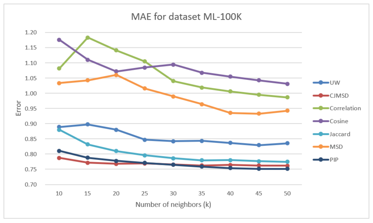
Figure 1 illustrates the prediction accuracy results obtained for the ML-100k dataset for the different methods being studied.

Figure 1 shows the results of the ML-100k dataset. When the $k$’s value is increased, UW has the performances significantly better than the traditional methods. The result shows that at $k = 50,$ our method has an increase of 15.30% in MAE against correlation and 18.94% in MAE against cosine and 11.35% against MSD. These improvements suggest increasing the number of user-item weight in the prediction process better reflects users’ true taste.

As seen in the bottom part of Figure 1, we also did the experiments to compare proposed methods with several state-of-art methods, including Jaccard, PIP, and CJMSD. Although there is no improvement in MAE against these methods, our method’s performance on the data set mL-100k is relatively very close. For instance, the difference between the UW and Jaccard results is only 7.86% at $k=50$.

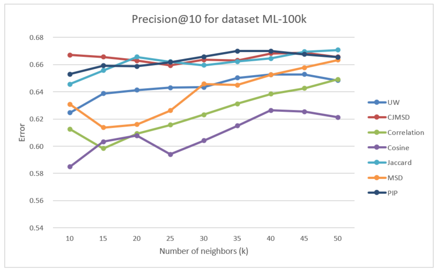
In Figure 2, we observed the precision of the seven prediction methods for a given $k$. It is clear from the figure that the precision increases as $k$ increases. At $k = 40$, our method is better than two traditional methods, 2.22% with correlation and 4.18% with cosine, and almost the same as the MSD.

Compared with CJMSD, PIP and Jaccard, UW underperforms in terms of precision. However, the difference in improvement is relatively small. Actually, it is only 0.02 lower than PIP’s best result, which is just 2.58%.

Here, in Figure 3, we observed the Recall of seven methods. As seen in Figure 3, the Recall of UW is significantly better than that of three different traditional methods (correlation, Cosine, MSD). Although the results of these three methods improve as $k$ increases, our method is significantly better for all values of k. At $k=40$, the improvement in recall for UW against cosine is 94.27%, almost double the cosine’s result. For the same $k$ value, the improvements against MSD and correlation are 33.92% and 55.78%. Compared with the state-of-art, our method is 2.4% better than Jaccard and fairly close to the other two methods.

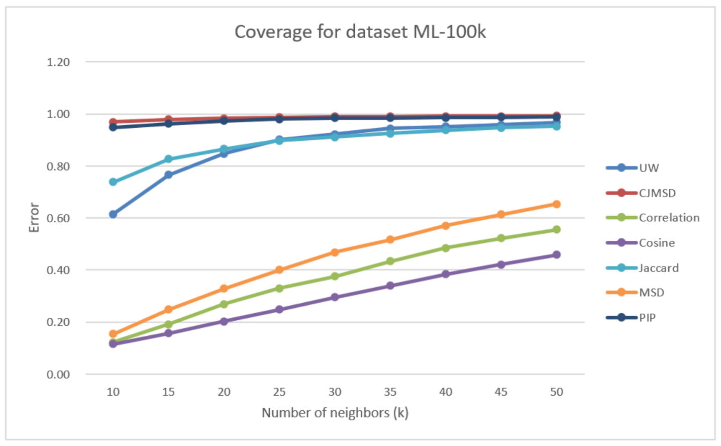
As seen in Figure 4, we observed that the prediction coverage of UW is significantly better than that of the three traditional methods. Our proposed method has 96.30% improvement against correlation, 147.37% improvement against cosine, and 66.53% improvement against MSD at $k=50$. The result of our methods is also closer to the result of CJMSD and PIP. For all the $k$ values higher than 30, our method has a better performance than Jaccard.

3.4.2. Results on ML-Latest-Small Dataset

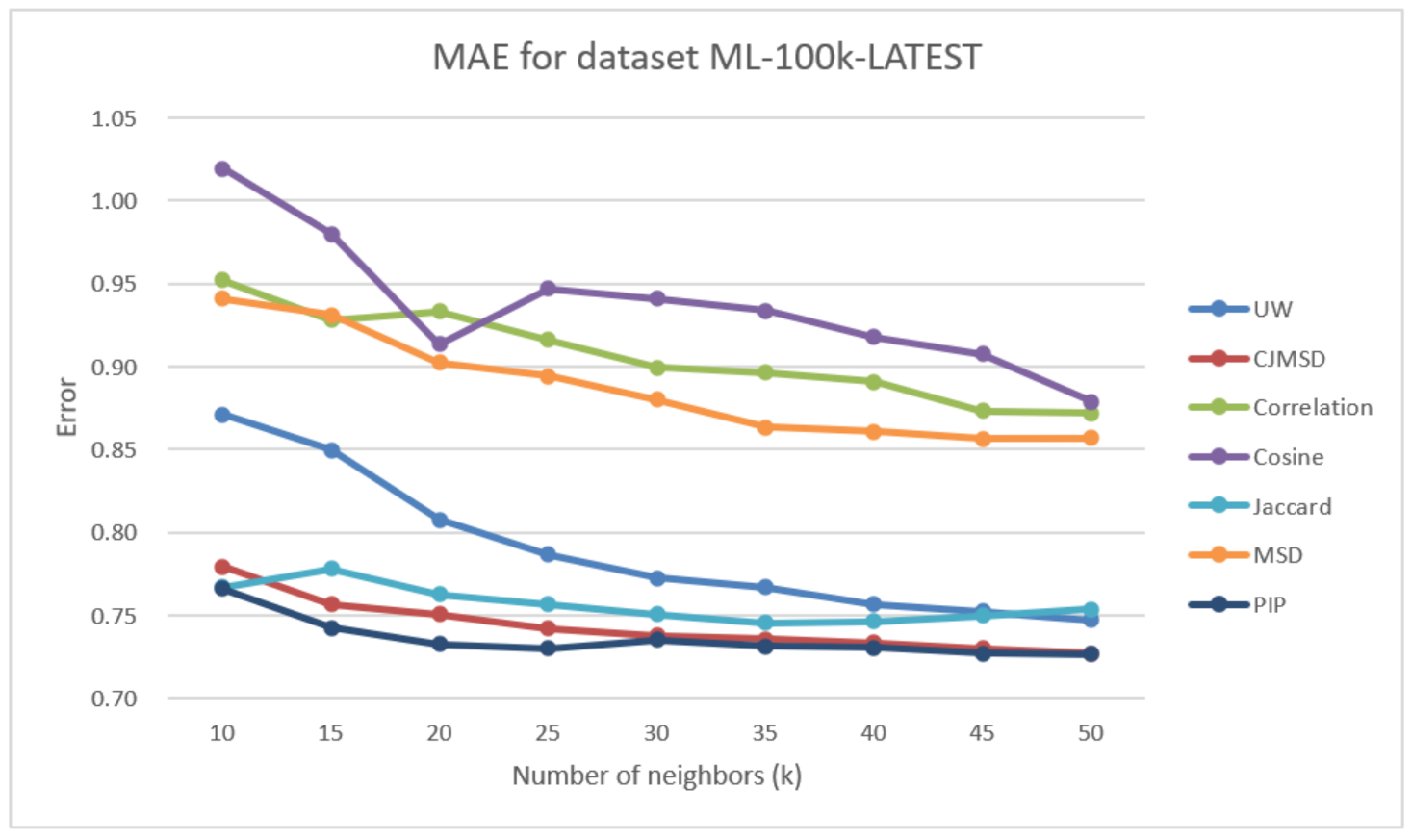
Figure 5 illustrates the prediction accuracy results obtained for the ML-latest-small dataset for the seven test methods.

Similar to the ML-latest-small dataset results, the relative improvements among different methods are roughly the same. The prediction accuracies of UW still have good performances among these methods. Our proposed method (UW) even beats Jaccard at $k=50$. The improvements in MAE against correlation, cosine, and MSD at $k=50$ are 14.32%, 14.99%, and 12.82%. The values of the user-item-weight matrix are much evenly spread across the items for this dataset. Meaning item features and user features are well represented. This could be due to items having more features (19 genres) than in the ML-100k dataset. In addition, users have more ratings per item in this dataset. Consequently, the weight-matrix has a much better representation of user features and items features, leading to better accuracy.

Similar to the results of experiments on the ML-100k dataset, state-of-art methods perform better than our method and traditional methods.

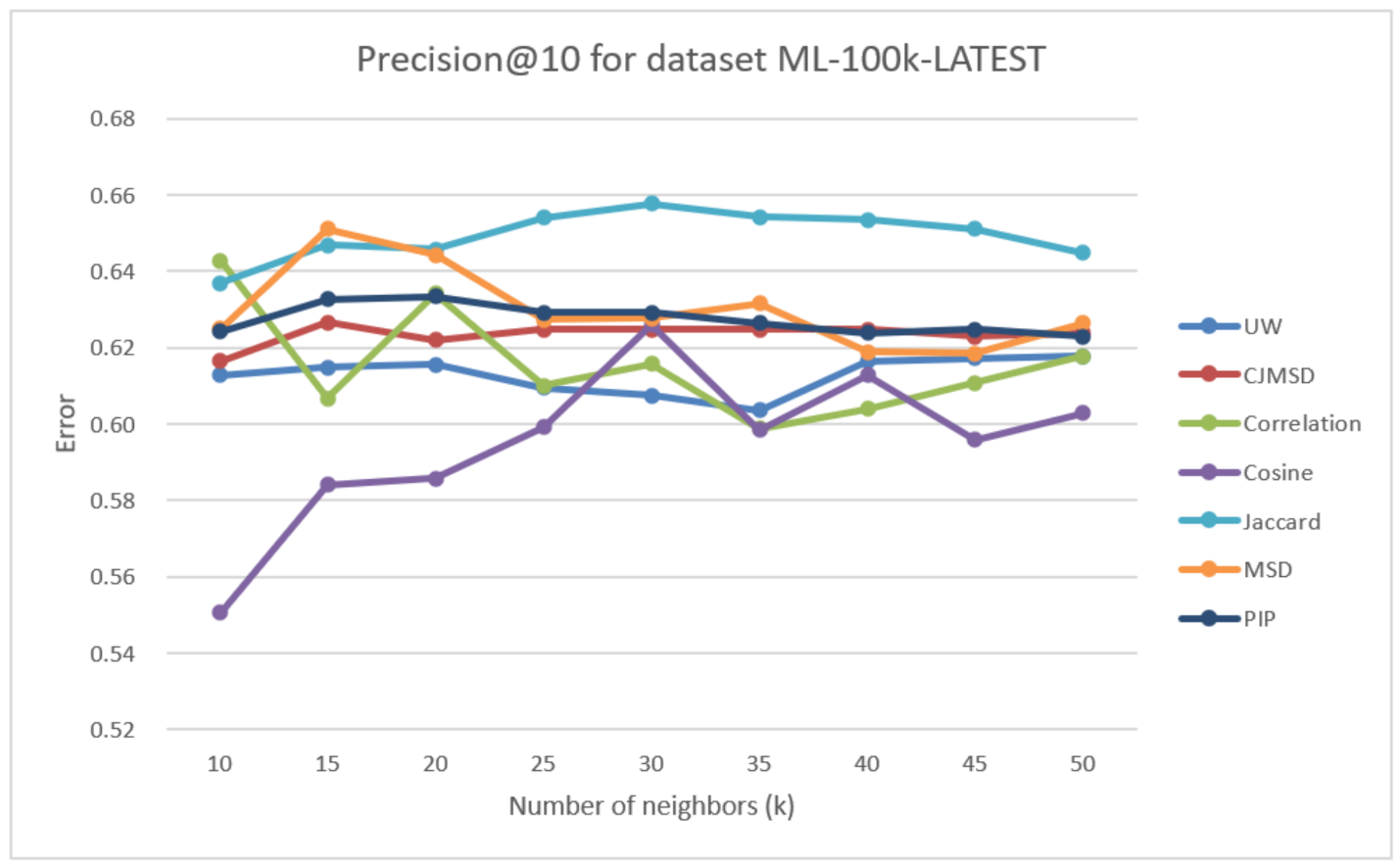
As seen in Figure 6, we observed the precision of the seven test methods at different $k$ values. In contrast to the previous dataset, there is more variance in the results for all the methods. However, as $k$ approaches 50, the precision of all the methods seems stuck around 0.62, except PIP (which is the best) and cosine (which is the worst).

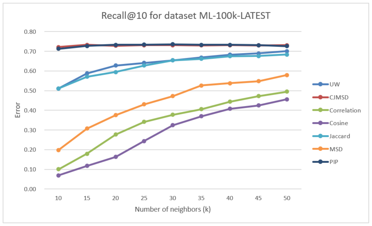
In Figure 7, we can see significantly better recall values compared with all the test methods except CJMSD and PIP. At $k=50$, the improvement against correlation, cosine, MSD and Jaccard are 41.49%, 53.65%, 20.92%, and 2.56%, respectively. The general trend for this data is the same as the previous dataset. The recall values increase as $k$ increases.

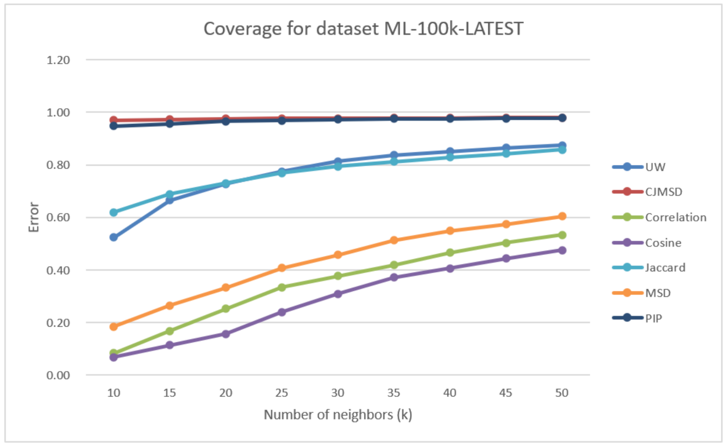
As seen in Figure 8, coverage of UW follows a similar trend as Jaccard. However, UW has better coverage as k values are increased. The performance improvements of UW at k = 50 against correlation, cosine, MSD, and Jaccard are 63.65%, 84.05%, 44.78%, and 1.84%. Although there is a gap between the performance of UW and the performances of JMSD and PIP, the gap narrows as the k value increases.

3.4.3. Results on ML-1m Dataset

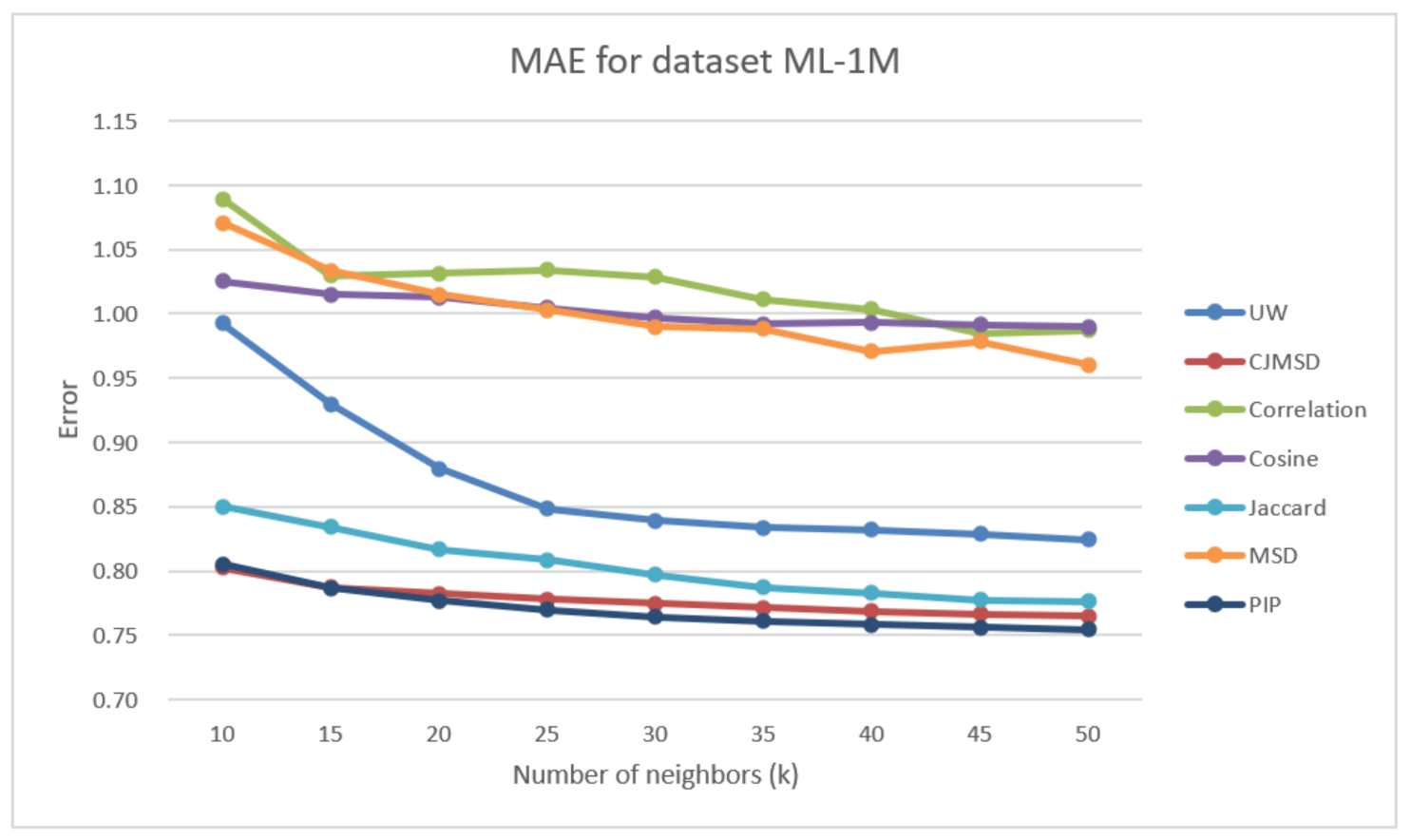
Figure 9 illustrates the prediction accuracy results obtained for the ML-1m dataset for the different methods being studied.

Similar to the results for the above two datasets, the relative improvements among different methods are roughly the same. UW’s prediction accuracy still has good performances among these methods, with an increase of 17.08% in MAE against correlation and 16.24% against cosine and 14.33% against MSD. Jaccard, JMSD and PIP perform better than our method. However, there is a significant decrease in the difference of performance with these methods as $k$ is increased.

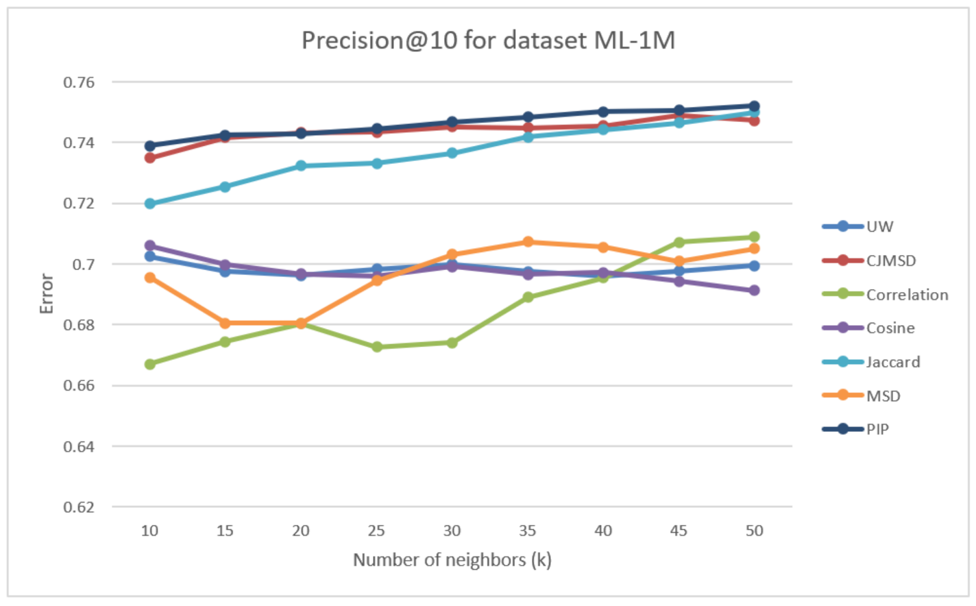
In Figure 10, we observed the Precision of the seven test methods. The proposed method’s precision stays around 0.7, despite the increase in k, and cosine follows a similar trend until it reaches $k= 50$, where precision falls further down. Correlation and MSD have better precision at a high $k$ value. Jaccard, JMSD, and PIP perform significantly better than the traditional methods.

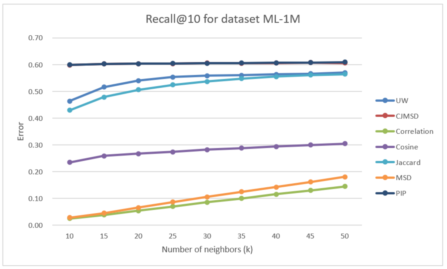
Although we do not have a good performance in Precision in this ML-1m data set, we have a significantly good Recall result. As seen in Figure 11, The recall of UW is significantly better than traditional kNN-based methods. This will gradually become apparent as the size of the dataset grows. Compared with three different traditional methods, the improvement against cosine is 91.99% while $k$ is equal to 40, the improvements against two other kNN-based methods, MSD and correlation, is 295.30% and 388.13%. Even compared with the state-of-art, our result is 1.48% better than Jaccard and fairly close to the other two methods.

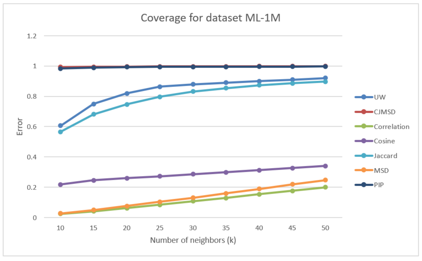
As seen in Figure 12, we observed that UW’s coverage is significantly better than the three traditional methods. The method’s performance has 485.69% improvement against correlation, 188.80% improvement against cosine, 380.11% improvement against MSD. Our method’s result is also close to CJMSD and PIP, as the figure above shows. While the chosen value of k is higher than 25, our method will have a better performance than Jaccard. Especially when $k$ is equal to 40, the improvement against Jaccard is 3.16%.

3.5. Sparsity of Weight Matrix

To compare the weight matrices’ sparsity among different methods, in Figure 10, we plot the number of empty entries in the weight matrix against the number of users. The dataset that we are used here is ML-100k.

As seen in Figure 13, for all the other methods (since the values for other methods are very close, they are superimposed), an increase in the number of users increases the sparsity of the weight matrices; however, for UW, the plot shows a flat zero, meaning the weight matrix is always full. This is due to the commonly rated item-genres (as each item has one or more genres) among the users. As discussed earlier, decreasing the sparsity is important as it impacts the accuracy of the predictions.

4. Discussion

Although the proposed method has a significantly better quality of perdition on all metrics against cosine, correlation, and MSD, it is not the same for PIP, CJMSD, and Jaccard. One of the main advantages of the proposed method is its ability to produce a unique prediction for users who have no neighbors in other test methods, which helps improve the coverage significantly. However, this is not the same as the cold-start problem where the user has not rated an item or an item has not been rated by any user. In these cases, our proposed methods will also fail as the weight matrix will have 0 entries for these users or items. Another problem with the proposed method is that the weight values are always positive, and prediction involves summing all the weighted ratings. This is not the case with correlation methods, where some similarity values are negative. Although users with negative similarities are less likely to be used while making predictions, prediction calculation involves summing them. Consequently, the weighted values are negated from the resulting prediction allowing the predictions to be a lower value. This is useful for predicting values for items the user does not like. We believe this is the main reason why the prediction accuracy of the proposed method is sometimes low. We plan to do future exploration in this avenue.

We also checked how a user’s weight vector affects the predictions. For instance, we choose user 496 (from the MovieLens 100k dataset), the weight score for item 499 is 0.106, suggesting the user and the item shares relatively similar categorical features. The first four entries for user-weight and item-weight vectors are 0.0, 0.0983, 0.0473, 0.0152, 0.0490 and 0.0,0.0947,0.046,0.008,0.069, respectively. The entries reflect the genres (action, adventure, animation, and children). For brevity, we did write all the entries in the vectors. During the recommendation process, neighbor weights are taking into account. The cumulative-weight value for 10 nearest-neighbors is 0.861. As a result, the items get at a rating score of 3.694. (which is usually rounded up to 4 stars). Therefore, we can easily explain why this item has been recommended. Unlike the traditional explainable recommenders that usually suggest "you liked this item because you liked X item", our system can notify the details of the item as well as the user’s preference. For example, “We think you’ll like this item because you don’t like action movies and this movie contain the right amount of adventure and animation. Also, other users like you enjoy this movie”.

In contrast to the correlation-based methods, our method considers all the items’ features while making the prediction. In correlation-based methods, these values are negated from the predicted value. We see this as unnecessary computation since we are only trying to find items that the user likes. In fact, in most of the implementation of correlation-based methods, these negative values are ignored. As seen in the results reporting in previous sections, our method has a significant advantage over other kNN-based methods.

5. Conclusions

This study proposed a new algorithm to improve the prediction quality in memory-based collaborative filtering and show the proposed method’s effectiveness using the MovieLens datasets. The basic idea is that we use the items’ genre information to find how much each user likes a specific item. The user-item relations are represented in the user-item-weight matrix. It is calculated by combining users’ specific categorical features and item-specific categorical features.

The user-item weights are different for each user-item pair. In contrast to the square-shaped similarity matrix used by the kNN method, the user-item-weight matrix is rectangular. Since the matrix is less sparse, the proposed method has better coverage than the kNN method. By experimental evaluations on three real benchmark datasets, we have shown that the proposed method can improve the prediction accuracy, precision, recall, and coverage. The method can make predictions in real time provided that the weight matrix is precomputed. One of the key advantages of the proposed method is that our method provides an explainable recommendation. In contrast to most of the explainable recommenders, our method shows how much a specific user likes a specific recommended item.

The major issue with the proposed method is that the prediction calculation only considers the addition of the weighted user rating. We plan to address this issue in our future work. However, our method can make predictions for the cases where kNN fails. This is a major advantage over other similarity-based collaborative filtering methods. Modern recommendation systems rely heavily on deep learning models. We are currently working on building a reinforcement learning model that incorporates item features to make predictions.

References

- Ricci, F.; Rokach, L.; Shapira, B.; Kantor, P.B. Recommender Systems Handbook; Springer Science and Business Media LLC: Berlin, Germany, 2011; pp. 1–35. [Google Scholar]
- Melville, P.; Mooney, R.J.; Nagarajan, R. Content-boosted collaborative filtering for improved recommendations. In Proceedings of the Eighteenth National Conference on Artificial Intelligence (AAAI-02), Edmonton, AB, Canada; 2002; pp. 187–192. [Google Scholar]
- Breese, J.S.; Heckerman, D.; Kadie, C. Empirical analysis of predictive algorithms for collaborative filtering. arXiv 2013, arXiv:1301.7363. Available online: https://arxiv.org/abs/1301.7363 (accessed on 14 May 2020).
- O’Donovan, J.; Dunnion, J. A framework for evaluation of information filtering techniques in an adaptive recommender system. In Proceedings of the International Conference on Intelligent Text Processing and Computational Linguistics, Seoul, Korea, 15–21 February 2004; pp. 502–506. [Google Scholar] [CrossRef]
- Tang, J.; Huan, L.; Liu, H. Social recommendation: A review. Soc. Netw. Anal. Min. 2013, 3, 1133. [Google Scholar] [CrossRef]
- Amazon.com, Inc. Available online: www.amazon.cn (accessed on 14 May 2020).
- JD.com, Inc. Available online: www.jd.com (accessed on 14 May 2020).
- Fayyaz, Z.; Ebrahimian, M.; Nawara, D.; Ibrahim, A.; Kashef, R. Recommendation Systems: Algorithms, Challenges, Metrics, and Business Opportunities. Appl. Sci. 2020, 10, 7748. [Google Scholar] [CrossRef]
- Billsus, D.; Pazzani, M.J. Learning Collaborative Information Filters. In Proceedings of the International Conference on Machine Learning (ICML), Madison, WI, USA, 24–27 July 1998; pp. 46–54. [Google Scholar]
- Golbandi, N.; Koren, Y.; Lempel, R. Adaptive bootstrapping of recommender systems using decision trees. In Proceedings of the fourth ACM international conference on Web search and data mining, Hong Kong, China, 9–12 February 2011; pp. 595–604. [Google Scholar] [CrossRef]
- Zhang, F.; Zhou, Q. HHT–SVM: An online method for detecting profile injection attacks in collaborative recommender systems. Knowledge-Based Syst. 2014, 65, 96–105. [Google Scholar] [CrossRef]
- Miyahara, K.; Pazzani, M.J. Improvement of collaborative filtering with the simple Bayesian classifier. Inf. Process. Soc. Japan 2002, 43, 3430–3437. [Google Scholar]
- Adomavicius, G.; Tuzhilin, A. Toward the next generation of recommender systems: A survey of the state-of-the-art and possible extensions. IEEE Trans. Knowl. Data Eng. 2005, 17, 734–749. [Google Scholar] [CrossRef]
- Ntoutsi, E.; Stefanidis, K.; Nørvåg, K.; Kriegel, H.-P. Fast group recommendations by applying user clustering. Proceedings of International Conference on Conceptual Modeling(ICCM), Florence, Italy, 15–18 October 2012; pp. 126–140. [Google Scholar]
- Moscato, V.; Picariello, A.; Sperli, G. An emotional recommender system for music. IEEE Intell. Syst. 2020, 1. [Google Scholar] [CrossRef]
- Amato, F.; Moscato, V.; Picariello, A.; Sperlí, G. KIRA: A System for Knowledge-Based Access to Multimedia Art Collections. In Proceedings of the 2017 IEEE 11th International Conference on Semantic Computing (ICSC), San Diego, CA, USA, 30 January–1 February 2017; pp. 338–343. [Google Scholar] [CrossRef]
- Yuan, Y.; Zahir, A.; Yang, J. Modeling Implicit Trust in Matrix Factorization-Based Collaborative Filtering. Appl. Sci. 2019, 9, 4378. [Google Scholar] [CrossRef] [Green Version]
- Zahir, A.; Yuan, Y.; Moniz, K. AgreeRelTrust—A Simple Implicit Trust Inference Model for Memory-Based Collaborative Filtering Recommendation Systems. Electronics 2019, 8, 427. [Google Scholar] [CrossRef] [Green Version]
- Montaner, M.; López, B.; De La Rosa, J.L. A Taxonomy of Recommender Agents on the Internet. Artif. Intell. Rev. 2003, 19, 285–330. [Google Scholar] [CrossRef]
- Lee, O.-J.; Jung, J.J. Explainable Movie Recommendation Systems by Using Story-Based Similarity. In Proceedings of the IUI Workshops, Tokyo, Japan, 7–11 March 2018. [Google Scholar]
- Zhang, Y.; Chen, X. Explainable Recommendation: A Survey and New Perspectives. Found. Trends® Inf. Retr. 2020, 14, 1–101. [Google Scholar] [CrossRef] [Green Version]
- Harper, F.M.; Konstan, J.A. The movielens datasets: History and context. ACM Trans. Interact. Intell. Syst. 2015, 5, 1–19. [Google Scholar] [CrossRef]
- Surprise, a Python Library for Recommender Systems. Available online: http://surpriselib.com (accessed on 14 May 2020).
- Ahn, H.J. A new similarity measure for collaborative filtering to alleviate the new user cold-starting problem. Inf. Sci. 2008, 178, 37–51. [Google Scholar] [CrossRef]
- Bobadilla, J.; Ortega, F.; Hernando, A.; Arroyo, Á. A balanced memory-based collaborative filtering similarity measure. Int. J. Intell. Syst. 2012, 27, 939–946. [Google Scholar] [CrossRef] [Green Version]
- Pitsilis, G.; Marshall, L.F. A model of trust derivation from evidence for use in recommendation systems; University of Newcastle upon Tyne, School of Computing Science: Newcastle upon Tyne, UK, 2004. [Google Scholar]
- Rendle, S.; Freudenthaler, C.; Schmidt-Thieme, L. Factorizing personalized markov chains for next-basket recommendation. In Proceedings of the 19th International Conference on World Wide Web, Raleigh, NC, USA, 26–30 April 2010; pp. 811–820. [Google Scholar]
Figure 1.
Prediction accuracy was obtained using different methods for the ML-100k data set. MAE—mean absolute error.
Figure 2.
Precision was obtained using different methods for the ML-100k data set.
Figure 3.
Recall obtained using different methods for the ML-100k data set.
Figure 4.
Coverage for seven methods on ML-100k data set.
Figure 5.
The prediction accuracy obtained using different methods for the ML-latest-small data set.
Figure 6.
The Precision obtained using different methods for the ML-latest-small data set.
Figure 7.
Recall obtained using different methods for the ML-latest-small data set.
Figure 8.
Coverage for seven methods on ML-latest-small data set.
Figure 9.
The prediction accuracy obtained using different methods for the ML-1m data set.
Figure 10.
The precision obtained using different methods for the ML-1m data set.
Figure 11.
Recall obtained using different methods for the ML-1m data set.
Figure 12.
Coverage for seven methods on ML-1m data set.
Figure 13.
The sparsity of the weight matrices versus the number of users for two methods.