Article

Green’s Functions of Multi-Layered Plane Media with Arbitrary Boundary Conditions and Its Application on the Analysis of the Meander Line Slow-Wave Structure

1
Key Laboratory of Science and Technology on High Power Microwave Sources and Technologies, Aerospace Information Research Institute, Chinese Academy of Sciences, Beijing 100190, China
2
School of Electronic, Electrical and Communication Engineering, University of Chinese Academy of Sciences, Beijing 100039, China
*
Author to whom correspondence should be addressed.
Submission received: 14 October 2021 / Revised: 2 November 2021 / Accepted: 4 November 2021 / Published: 8 November 2021
(This article belongs to the Special Issue High-Frequency Vacuum Electron Devices)

Abstract

:
A method was proposed for solving the dyadic Green’s functions (DGF) and scalar Green’s functions (SGF) of multi-layered plane media in this paper. The DGF and SGF were expressed in matrix form, where the variables of the boundary conditions (BCs) can be separated in matrix form. The obtained DGF and SGF are in explicit form and suitable for arbitrary boundary conditions, owing to the matrix form expression and the separable variables of the BCs. The Green’s functions with typical BCs were obtained, and the dispersion characteristic of the meander line slow-wave structure (ML-SWS) is analyzed based on the proposed DGF. The relative error between the theoretical results and the simulated ones with different relative permittivity is under 3%, which demonstrates that the proposed DGF is suitable for electromagnetic analysis to complicated structure including the ML-SWS.

1. Introduction

Since the exact results of the two-layered planar dielectric model were deduced [1], more and more people have been engaged in research of the electromagnetic field for multi-layered media [2,3,4,5,6,7,8,9,10,11,12,13,14,15,16,17,18,19,20,21,22], which has been widely utilized for the analysis of dielectric waveguides, printed circuit boards, antennas and sensors [23,24,25,26].
The Green’s functions, including dyadic Green’s functions (DGF) and scalar Green’s functions (SGF), are powerful tools in electromagnetic theory [2,3,4], because the relationship between the field and excitation sources can be easily described by them. As a result, many years of effort have been devoted to obtaining Green’s functions for inhomogeneous media [3,4,5,6,7,8,9,10,11,12,13,14,15,16,17,18,19,20,21,22] There are many approximation and numerical methods that have been utilized for calculating the DGF and SGF, such as the finite sum superposition method [3], the total least squares method [4], the fast full-mode method [5], the numerical modified steepest descent path method [5] and the numerically stable analysis method [6]. In addition, the pure theoretical derivations of Green’s functions for the stratified media, without numerical approximation and error, were also pursued for a long time [7,8,9,10,11,12,13,14,15,16,17,18,19,20,21,22]
The form of the dyadic Green’s function has been presented based on the methods of generation function expansions [7,8,9,10,11,12,13,14,15] (the generation functions were called vector wave functions in [7,8,9], eigen-functions in [10,12,13,14,15] and solenoidal Hausen vectors in [11]), and this form can also be used in multi-layered media conditions [8,9,10,11,12,13,14,15]. If these traditional generation functions, such as those in [8], are selected to obtain the DGF, the boundary conditions (BCs) between the adjacent layers will be satisfied by another method, such as the method of scattering superposition [9,10]. Consequently, the equations built from the boundary conditions may be complicated and the results may be not in explicit form. The method of scattering superposition is direct with explicit physical meanings for multi-layered media [7]. However, it will be complicated when the number of layers is increased. Instead, if the BCs has been contained in the generation function with explicit form, the corresponding Green’s function can be simple and in explicit form.
In addition, methods such as the perturbative approach [16], operator theories [18,19,20], wave superposition [21] and transmission line theories [17,18,21,22] are also introduced for obtaining the Green’s function and exactly analyzing the multi-layered media. Unfortunately, the applications of these results are limited, owing to the specified boundary conditions at two ends of the multi-layered media [18]. In [21], although the DGF of multi-layered media is obtained with undefined boundary conditions at two ends, the DGF is deduced in the rectangular waveguide, whose length is assumed infinite, and the direction of the stratified media must be defined in consistence with that of the guided wave’s propagation. In [20,21,22], the obtained Green’s function of multi-layered plane media contain the BCs between the adjacent layers, but they do not contain the BCs at the top and the bottom of multi-layered media. When they are utilized to analyze the specified structures, the BCs at two ends of multi-layered media must be considered, and the corresponding equations will be built from the BCs and these Green’s functions [18]. As a result, the equations of the structure base on the Green’s function in [18] may be more complicated, because BCs at two ends may add the number of the equation.
In this paper, a method was proposed for obtaining the Green’s functions of multi-layered media with arbitrary boundary conditions, including dyadic Green’s functions and scalar ones. In this method, the Green’s functions consist of the generation functions. In the process of deducing the generation functions, the BCs between the adjacent layers and at two ends have been considered, and are represented by a series of variables. These variables of the BCs can be separated in matrix form. Correspondingly, the DGF and SGF were obtained in explicit form with matrixes, and corresponding equations built from BCs at the top and the bottom of the multi-layered media are independent and easy to solve, which means that the equations of the structure based on the proposed DGF may be more simple with clearer physical characteristics and that the formulae may be expressed with the computer code more friendly.
In Section 2, the proposed method was discussed. The typical BCs, such as metal boundary conditions, radiation boundary conditions and their combinations, were discussed in Section 3, respectively. Furthermore, the application on the dispersion analysis of a meander line slow-wave structure is given in Section 4. The effect of relative permittivity on the dispersion is discussed, and the results of theoretical calculation are compared with those of the simulation. In addition, conclusions are drawn in Section 5.
It should be noted that, in this paper, the y-axis is regarded as the referent direction, k 0 is the wave number in free space, k c is the eigenvalue in the cross section to referent direction, and δ i , j is the Kronecker delta function. Moreover, the symbol will be replaced by , if the corresponding eigenvalue is continuous.

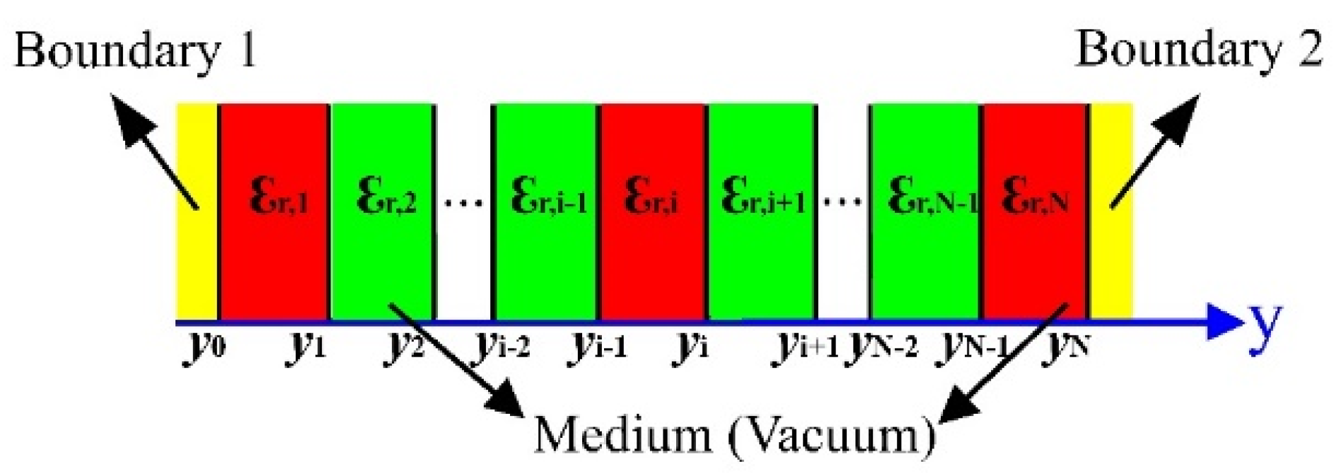
2. The DGF and SGF of Multi-Layered Plane Media with Arbitrary Boundaries

Figure 1 shows the geometry of multi-layered media, which is stratified along the y-axis and can be divided into N layers.
ε r = ε r , j   when   y ( y j 1 , y j ] j = 1 , 2 , , N
where ε r ( ε r , j ) is the relative permittivity (in the jth layer). y j 1 and y j are the two edge values of the jth layer at y-axis. The two bottom boundaries are marked “Boundary 1” and “Boundary 2”, respectively.
Owing to the principle of field superposition, most sources can be regarded as a sum of point sources. Therefore, a 3D point source δ is selected as the excitation source. Assuming that the excitation source, marked with “ ”, is in the ith layer, and choosing y-axis as the referent direction, the SGF G j ( R , R ) for the jth layer satisfies the Helmholtz equation as follows:
{ 2 G j ( R , R ) + ε r , j k 0 2 G j ( R , R ) = 0 , j i , j = 1 , 2 , , N 2 G i ( R , R ) + ε r , i k 0 2 G i ( R , R ) = δ ( R R ) , j = i
Furthermore, the GF can be expressed as the sum of TM and TE components to the referent direction (y-axis), namely,
G j ( R , R ) = G m j ( R , R ) + G n j ( R , R )
The boundary conditions at y = y j can be written as:
{ ε r , j G m j ( R , R ) = ε r , j + 1 G m j + 1 ( R , R ) , j = 1 , 2 , , N 1 1 ε r , j y G m j ( R , R ) = 1 ε r , j + 1 y G m j + 1 ( R , R ) G n j ( R , R ) = G n j + 1 ( R , R ) y G n j ( R , R ) = y G n j + 1 ( R , R )
Because the shape of cross section is uniform along the y-axis, considering the isotropic and lossless media, G n m j ( R , R ) can be expressed according to function f n m , j i ( y , y ) for different transverse eigenvalues k c [18].
G n m j ( R , R ) = k c g n m · f n m , j i ( y , y )
where, index i represents that the excitation source is in the ith layer and g n m is the coefficient of the series.
The f n m , j i ( y , y ) in Equation (5) can be described as follows:
d 2 d y 2 f n m , j i ( y , y ) + ( ε r , j k 0 2 k c 2 ) f n m , j i ( y , y ) = 0   when   y ( y j 1 , y j ) , j i , j = 1 , 2 , , N
d 2 d y 2 f n m , i i ( y , y ) + ( ε r , i k 0 2 k c 2 ) f n m , i i ( y , y ) = F n m g n m * ( x , z ) δ ( y y )   when   y ( y i 1 , y i )
where the F n m is the normalized coefficient, and Equation (4) can be simplified, when y = y j
{ ε r , j f m , j i ( y , y ) = ε r , j + 1 f m , j + 1 i ( y , y ) , f n , j i ( y , y ) = f n , j + 1 i ( y , y ) 1 ε r , j d d y f m , j i ( y , y ) = 1 ε r , j + 1 d d y f m , j + 1 i ( y , y ) ,   d d y f n , j i ( y , y ) = d d y f n , j + 1 i ( y , y )
According to the operator theories, the electromagnetic field can be analyzed in the Hilbert space, and the function space consisting of orthonormal basis functions, { sin ( k y ) cos ( k y ) } , is complete [18].
Assuming that the f n m , j i ( y , y ) can be written as:
{ f n m , k i ( y , y ) = C n m [ S y , k + ( y ) ] [ a n m , k b n m , k ] T , y k 1 y y k , y y f n m , l i ( y , y ) = C n m [ S y , l ( y ) ] [ c n m , l d n m , l ] T , y l 1 y y l , y y
where, the C n m is the weight factor, 1 k i l N ,
C n m = F n m g n m * ( x , z )
k y , i = ( ε r , i k 0 2 k c 2 )
{ [ S y , j + ( y ) ] = [ sin ( k y , j ( y y j 1 ) ) cos ( k y , j ( y y j 1 ) ) ] [ S y , j ( y ) ] = [ sin ( k y , j ( y j y ) ) cos ( k y , j ( y j y ) ) ]
Putting Equations (9)–(12) into Equation (8), one can get:
[ a n m , k + 1 b n m , k + 1 ] = [ T n m , k ] [ a n m , k b n m , k ] , [ c n m , l d n m , l ] = [ R n m , l ] [ c n m , l + 1 d n m , l + 1 ]
where matrixes [ T m , k ] , [ T n , k ] , [ R m , l ] and [ R n , l ] are provided in Appendix A.
For brief expression, matrixes [ A n m , i ] and [ B n m , i ] can be defined:
[ A n m , i ] = T n m , i 1 T n m , i 2 T n m , 1 T n m , 0 = [ A n m , i 1 A n m , i 2 A n m , i 3 A n m , i 4 ] ,   [ B n m , i ] = R n m , i R n m , i + 1 R n m , N 1 R n m , N = [ B n m , i 1 B n m , i 2 B n m , i 3 B n m , i 4 ]
Therefore, Equation (9) can be rewritten as
f n m , j i ( y , y ) = C n m { [ S y , j + ( y ) ] [ A n m , j ] [ a n m , 1 b n m , 1 ] T , y j 1 y y j , y y [ S y , j ( y ) ] [ B n m , j ] [ c n m , N d n m , N ] T , y j 1 y y j , y y
Here, the f n m , j i ( y , y ) can be represented as:
f m , j i ( y , y ) = C m M j ( y ) ( U i * ( y ) ) T , f n , j i ( y , y ) = C n N j ( y ) ( V i * ( y ) ) T
where,
{ M j ( y ) = { [ S y , j + ( y ) ] [ A m , j ] , y y [ S y , j ( y ) ] [ B m , j ] , y y   , y j 1 y y j U i * ( y ) = { [ a m , 1 b m , 1 ] , y y [ c m , N d m , N ] , y y   , y i 1 y y i N j ( y ) = { [ S y , j + ( y ) ] [ A n , j ] , y y [ S y , j ( y ) ] [ B n , j ] , y y , y j 1 y y j V i * ( y ) = { [ a n , 1 b n , 1 ] , y y [ c n , N d n , N ] , y y , y i 1 y y i
As a result, SGF G j ( R , R ) can be represented as
G j ( R , R ) = k c ( g m ( x , z ) · ( C m M j ( y ) ( U i * ( y ) ) T ) + g n ( x , z ) · ( C n N j ( y ) ( V i * ( y ) ) T ) )
Furthermore, consider the Equation (10) and define the generating functions as:
{ φ m ( R ) = g m ( x , z ) M j ( y ) , ϕ m * ( R ) = g m * ( x , z ) U i * ( y ) φ n ( R ) = g n ( x , z ) N j ( y ) , ϕ n * ( R ) = g n * ( x , z ) V i * ( y )
where g m * ( x , z ) and g n * ( x , z ) are the conjugate functions of g m ( x , z ) and g n ( x , z ) , respectively. Note that the concrete mathematical form of g n m ( x , z ) depends on coordinate systems and boundary conditions in the x-z plane. In a Cartesian coordinate system, g n m ( x , z ) can be expressed by basic functions systems { sin ( k x ) cos ( k x ) } or { e i k x } . Then, the SGF G j ( R , R ) can be written in a usual expression:
G j ( R , R ) = k c ( F m φ m ( R ) ( ϕ m * ( R ) ) T + F n φ n ( R ) ( ϕ n * ( R ) ) T )
In addition, the DGF G j ( R , R ) can be expressed in the same form as that in [9]:
G j ( R , R ) = y ^ y ^ ε r , i k 0 2 δ ( R R ) + k c ( F n k c 2 ( ( × ( φ n ( R ) y ^ ) ) ( × ( ( ϕ n * ( R ) ) T y ^ ) ) ) ) + k c ( F m k c 2 k 0 2 ε r , j ε r , j ( × × ( φ m ( R ) y ^ ) ) ( × × ( ( ϕ m * ( R ) ) T y ^ ) ) )
Considering normalized conditions, the point source equations could be written as below:
{ f n m , k i ( y , y ) f n m , l i ( y , y ) = 0 d d y f n m , k i ( y , y ) d d y f n m , l i ( y , y ) = 1 , y = y , k = l = i
then
[ S y , i + ( y ) ] T [ A n m , i ] [ a n m , 1 b n m , 1 ] = [ S y , i ( y ) ] T [ B n m , i ] [ c n m , N d n m , N ] = k y , i [ c n m , N d n m , N ] [ B n m , i ] T [ D i ] [ A n m , i ] [ a n m , 1 b n m , 1 ] T
where [ D i ] is given in Appendix A.
Assume that variables b m , 1 , d m , N , a n , 1 , and c n , N are not zero, and they can be presented easily in matrix form:
{ b m , 1 = [ S y , i ( y ) ] [ B m , i ] [ c m , N d m , N 1 ] T / ( k y , i I m , i ) , d m , N = [ S y , i + ( y ) ] [ A m , i ] [ a m , 1 b m , 1 1 ] T / ( k y , i I my , i ) a n , 1 = [ S y , i ( y ) ] [ B n , i ] [ 1 d n , N c n , N ] T / ( k y , i I n , i ) , c n , N = [ S y , i + ( y ) ] [ A n , i ] [ 1 a n , 1 b n , 1 ] T / ( k y , i I ny , i )
I m y , i = [ c m , N d m , N 1 ] [ B m , i ] T [ D i ] [ A m , i ] [ a m , 1 b m , 1 1 ] T , I n y , i = [ 1 d n , N c n , N ] [ B n , i ] T [ D i ] [ A n , i ] [ 1 b n , 1 a n , 1 ] T
It is worth noting that variables a m , 1 , b m , 1 , c m , N , d m , N , a n , 1 , b n , 1 , c n , N and d n , N can be exactly deduced by the source conditions Equation (23) and conditions of boundary 1 and 2.

3. Typical Boundary Conditions and Examples

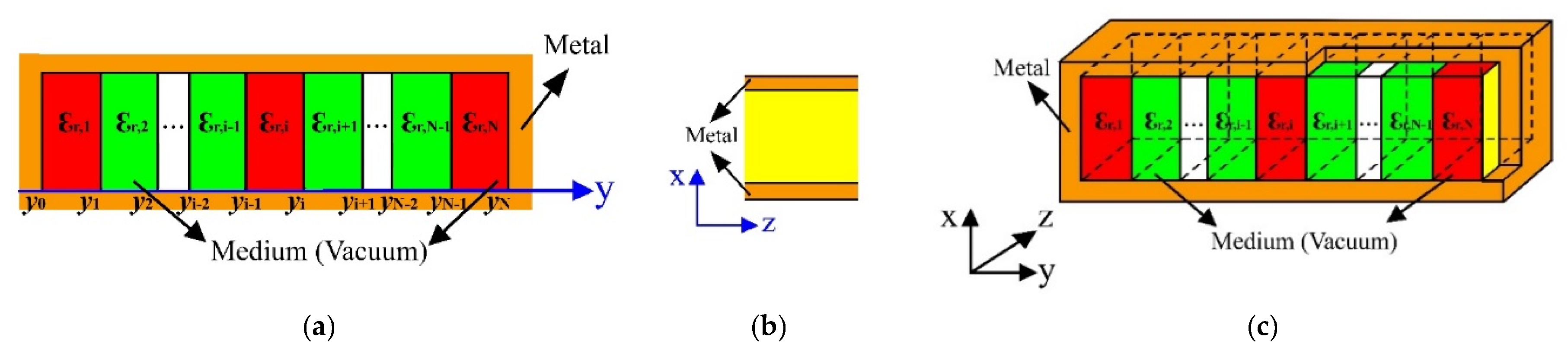
3.1. Metal Boundary Conditions

The typical boundaries are metal conditions. If boundary 1 and 2 are regarded as the metal conditions, the boundary equations can be derived as
d d y f m , j i ( y , y ) = 0 ,   and   f n , j i ( y , y ) = 0 , j = 1 , y = y 0   o r   j = N , y = y N
As a consequence,
a m , 1 = c m , N = b n , 1 = d n , N = 0
Bringing Equation (27) into source Equations (24) and (25), the rest of variables can be confirmed:
{ b m , 1 = [ S y , i ( y ) ] [ B m , i ] [ 0 1 ] T / ( k y , i I m , i ) , d m , N = [ S y , i + ( y ) ] [ A m , i ] [ 0 1 ] T / ( k y , i I m , i ) a n , 1 = [ S y , i ( y ) ] [ B n , i ] [ 1 0 ] T / ( k y , i I n , i ) , c n , N = [ S y , i + ( y ) ] [ A n , i ] [ 1 0 ] T / ( k y , i I n , i )
where
I m , i = [ 0 1 ] [ B m , i ] T [ D i ] [ A m , i ] [ 0 1 ] T , I n , i = [ 1 0 ] [ B n , i ] T [ D i ] [ A n , i ] [ 1 0 ] T
Then the SGF and the DGF can be written easily, according to Equations (20) and (21).

Example: A Rectangular Waveguide Laterally Filled with Multi-Layered Media

In Figure 2, the rectangular waveguide is laterally filled with multi-layered plane media along the y-axis. The guided wave is along the z-axis. As a result,
g m ( x , z ) = sin ( k x x ) e i h z , g n ( x , z ) = cos ( k x x ) e i h z , F m = 2 / ( π b ) , F n = 2 ( 2 δ k c , 0 ) / ( π b ) , k x = p π / b
where b is the height of the rectangular waveguide at x-axis.
As mentioned above, the DGF and GF can be exactly given by Equations (20) and (21).
Moreover, one can define N = 2, k y , 1 = β 2 , y 0 = 0 , y 1 = d , y 2 = a , ε r , 2 k 0 2 = k 1 2 , ε r , 1 k 0 2 = k 2 2 , k c 2 = k x 2 + h 2 , F = 1 / ( 2 π b ) , and the excitation source in the second layer (i = 2). The DGF in the first layer can be written as:
G 1 ( R , R ) = P ( ( × ( sin ( k y , 1 ( y y 0 ) ) g n ( x , z ) y ^ ) ) ( × ( sin ( k y , 2 ( y 2 y ) ) g n * ( x , z ) y ^ ) ) ( k y , 2 sin ( k y , 1 ( y 1 y 0 ) ) cos ( k y , 2 ( y 2 y 1 ) ) + k y , 1 cos ( k y , 1 ( y 1 y 0 ) ) sin ( k y , 2 ( y 2 y 1 ) ) ) + ( × × ( cos ( k y , 1 ( y y 0 ) ) g m ( x , z ) y ^ ) ) ( × × ( cos ( k y , 2 ( y 2 y ) ) g m * ( x , z ) y ^ ) ) ( ε r , 2 k y , 1 sin ( k y , 1 ( y 1 y 0 ) ) cos ( k y , 2 ( y 2 y 1 ) ) + ε r , 1 k y , 2 cos ( k y , 1 ( y 1 y 0 ) ) sin ( k y , 2 ( y 2 y 1 ) ) ) ) π b k 0 2 ( ( p π / b ) 2 + h 2 ) ( 1 + δ 0 ) d h
which is consistent with the results in [7].
As for the rectangular cavity filled with multi-layered plane media, Equation (30) is supposed to be replaced as follows, respectively:
g m ( x , z ) = sin ( k x x ) sin ( h z ) , g n ( x , z ) = cos ( k x x ) cos ( h z ) , F m = 4 / ( a b ) , F n = 4 ( 2 - δ k c , 0 ) / ( a b ) , k x = p π / b , h = q π / a
where a is the width of the rectangular cavity at z-axis.

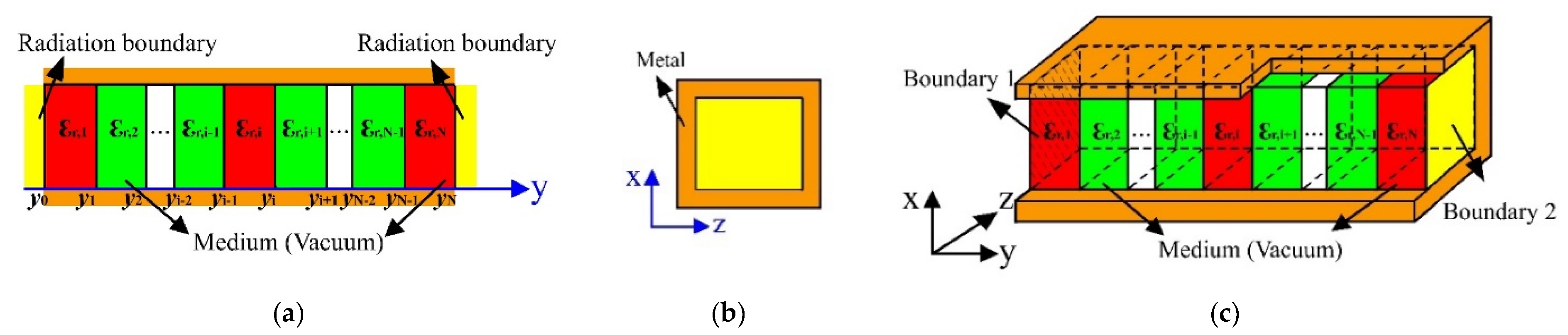
3.2. Infinite Radiation Boundary Conditions

While both boundaries 1 and 2 in Figure 1 are infinite radiation boundaries, the boundary equations are
lim y 0 ( y s 1 2 ( d d y f n m , 1 i ( y , y ) + i k y , 1 f n m , 1 i ( y , y ) ) ) | y = y 0 = 0 , lim y N ( y s 1 2 ( d d y f n m , N i ( y , y ) i k y , N f n m , N i ( y , y ) ) ) | y = y N = 0
Therefore, variables of the BC at two ends can be obtained:
{ a n m , 1 = [ S y , i ( y ) ] [ B n m , i ] [ 1 i ] T / ( k y , i I n m , i ) ,   b n m , 1 = [ S y , i ( y ) ] [ B n m , i ] [ i 1 ] T / ( k y , i I n m , i ) c n m , N = [ S y , i + ( y ) ] [ A n m , i ] [ 1 i ] T / ( k y , i I n m , i ) ,   d n m , N = [ S y , i + ( y ) ] [ A n m , i ] [ i 1 ] T / ( k y , i I n m , i )
where
I n m , i = [ i 1 ] [ B n m , i ] T [ D i ] [ A n m , i ] [ i 1 ] T
Hence, the SGF and the DGF can also be written, according to Equations (20) and (21).

Example: A Rectangular Waveguide Longitudinally Filled with Multi-Layered Media

The rectangular waveguide longitudinally filled with multi-layered media is exhibited in Figure 3, which is stratified along the y-axis. Therefore,
g m ( x , z ) = sin ( k x x ) sin ( h z ) , g n ( x , z ) = cos ( k x x ) cos ( h z ) , F m = 4 / ( a b ) , F n = 4 ( 2 δ k c , 0 ) / ( a b ) , k x = p π / b , h = q π / a
where b is the height of the rectangular waveguide at x-axis, and a is the width of the rectangular waveguide at z-axis.

3.3. Metal and Infinite Radiation Boundary Conditions

Assuming that boundary 1 is metal and boundary 2 satisfies the infinite radiation condition in Figure 1, then
d d y f m , 1 i ( y , y ) | y = y 0 = 0 , f n , 1 i ( y , y ) | y = y 0 = 0 , lim y N ( y s 1 2 ( d d y f n m , N i ( y , y ) i k y , N f n m , N i ( y , y ) ) ) | y = y N = 0
Therefore,
a m , 1 = 0 , c m , N = i d m , N , b n , 1 = 0 , d n , N = i c n , N
Equations (24) and (25) can be derived as:
{ b m , 1 = [ S y , i ( y ) ] [ B m , i ] [ i 1 ] T / ( k y , i I m , i ) , d m , N = [ S y , i + ( y ) ] [ A m , i ] [ 0 1 ] T / ( k y , i I m , i ) a n , 1 = [ S y , i ( y ) ] [ B n , i ] [ 1 i ] T / ( k y , i I n , i ) , c n , N = [ S y , i + ( y ) ] [ A n , i ] [ 1 0 ] T / ( k y , i I n , i )
where
I m , i = [ i 1 ] [ B m , i ] T [ D i ] [ A m , i ] [ 0 1 ] T , I n , i = [ 1 i ] [ B n , i ] T [ D i ] [ A n , i ] [ 1 0 ] T
The undetermined variables have been derived, and the corresponding SGF and DGF can be written, according to Equations (20) and (21).

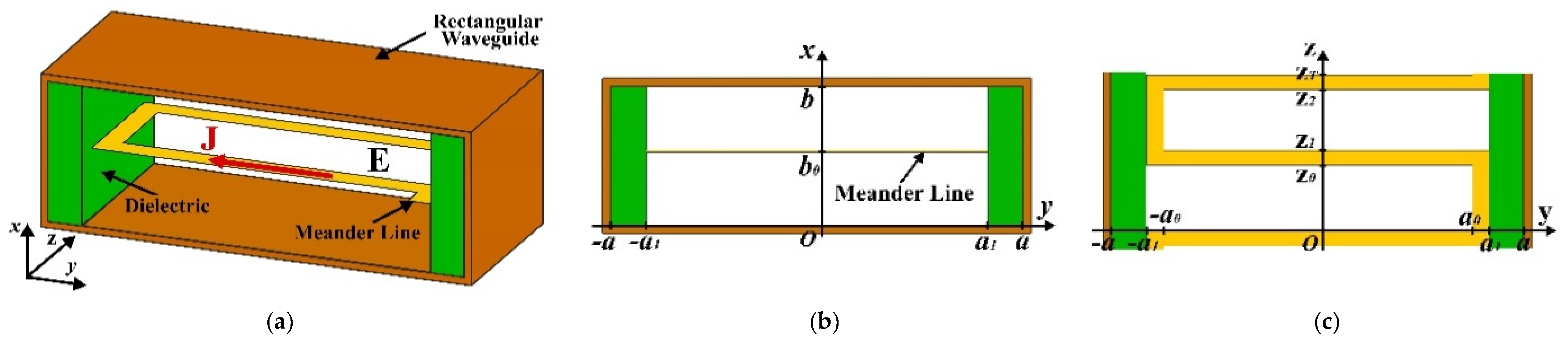
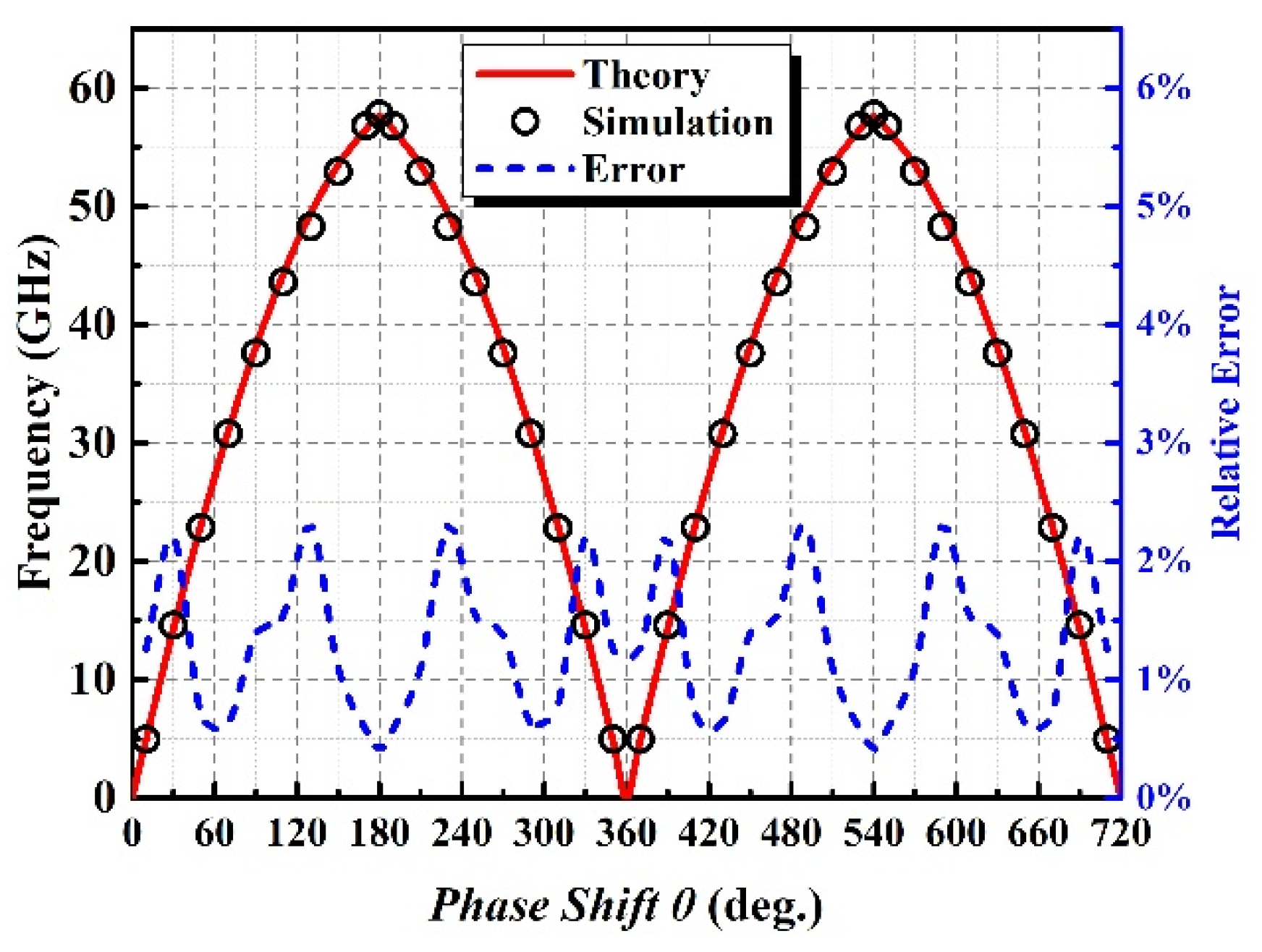
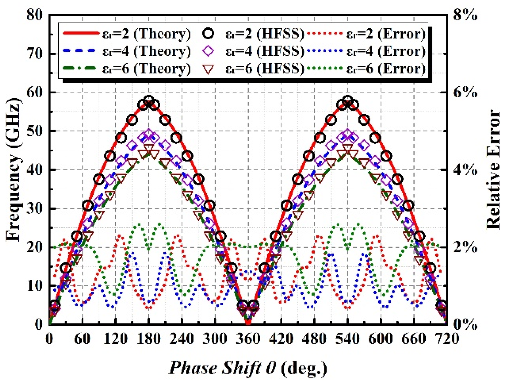
4. Application on the Dispersion Analysis for a Meander Line Slow-Wave Structure

As shown in Figure 4, the meander line slow-wave structure (ML-SWS) is composed of a meander line and a dielectric loaded waveguide. Here, the meander line is clamped with dielectrics, whose relative permittivity is ε r . For easy calculation, the thickness of the meander line is regarded as zero here. The parameters of the ML-SWS are given in Table 1.
According to the metal boundary condition, the tangential electric field E on the surface of the meander line should be zero.
E ( R ) = 0 , R Meander   Line
According to [9], the electric field E ( R ) can be written as:
E ( R ) = i ω μ V G ( R , R ) · J ( R ) d V
where G is the DGF of multi-layered plane media, which can be obtained as mentioned before. J is a current source along the meander line. Here, the current source can be expanded with sets of Ritz basic functions φ D , s such as the electric fields [27]:
J D = s = 0 A D , s φ D , s
where subscript “D” represents the direction of the current J and A D , s is a coefficient.
Bringing Equations (42) and (43) into Equation (41), the electromagnetic field expressions can be obtained. The expressions includes three sets of { A D , s } , position vector R and { ω , θ } , where ω is wave frequency and θ is the phase shift in a period.
Moreover, the cross product of Equation (41) with Ritz basic functions can be expressed in matrix form [28]:
[ Y ] [ A ] = 0
As a result, the dispersion function of the ML-SWS can be obtained as:
| Y | = 0
The dispersion characteristic of the ML-SWS can be obtained by Equation (45), where the upper range of both parameters s and t are 0 to 2. This calculation procedure can be performed in 2.4 min, which is only one-quarter of the time cost by HFSS code.
Based on the derived DGF of multi-layered plane media, the dispersion characteristics of the ML-SWS can be obtained, as shown in Figure 5. The obtained theoretical results are also compared with the simulated results from HFSS code. Furthermore, the relative error between them is under 3%, which is marked with a dashed line.
Moreover, the effect from the relative permittivity ( ε r ) of the dielectric is also studied, as shown in Figure 6. The upper cut-off frequency of the mode with the larger relative permittivity is smaller than that with the lower one. With the relative permittivity increasing, phase velocity decreases accordingly. The relative error between the theoretical results and simulated results from HFSS code are also within 3%, which indicates the theoretical results and simulated results with different relative permittivity are in good agreement.

5. Conclusions

A method for obtaining the Green’s functions of multi-layered plane media has been proposed in this paper. In this method, the Green’s functions consist of the generation functions. In the process of deducing the generation functions, the boundary conditions between the adjacent layers and at two ends have been considered, which are represented by a series of separable variables. Because these variables are separated in matrix form, the corresponding boundary equations can be independent. Consequently, the form of the generation functions and the obtained Green’s functions can be explicit and can be in consistence of different boundary conditions, and the corresponding expression can be expressed with the more friendly computer code.
Moreover, both the dyadic Green’s functions (DGF) and scalar Green’s functions (SGF) have been obtained. The obtained results are in good agreement with the predecessors’ works.
Furthermore, as the application, a ML-SWS with different relative permittivity has been analyzed. The calculation procedure can be performed in 2.4 min, which is only one-quarter of the time cost by HFSS code. The relative error between the theoretical results and the simulated ones with different relative permittivity is under 3%, which demonstrates that the proposed DGF can be suitable for electromagnetic analysis of complicated structures, including the ML-SWS.

Author Contributions

Conceptualization, Z.W., J.L. and W.L.; methodology, Z.W.; software, Z.W.; validation, Z.W. and W.L.; formal analysis, Z.W.; investigation, Z.W.; resources, Z.W.; data curation, Z.W.; writing—original draft preparation, Z.W.; writing—review and editing, Z.W. and J.L.; visualization, Z.W.; supervision, Z.W.; project administration, J.L. All authors have read and agreed to the published version of the manuscript.

Funding

This research received no external funding

Conflicts of Interest

The authors declare no conflict of interest.

Appendix A

The matrixes [ T m , k ] , [ T n , k ] , [ R m , l ] , [ R n , l ] and [ D i ] are defined as follows:
[ T m , k ] = [ ε r , k + 1 ε r , k k y , k k y , k + 1 cos ( k y , k ( y k y k 1 ) ) ε r , k + 1 ε r , k k y , k k y , k + 1 sin ( k y , k ( y k y k 1 ) ) ε r , k ε r , k + 1 sin ( k y , k ( y k y k 1 ) ) ε r , k ε r , k + 1 cos ( k y , k ( y k y k 1 ) ) ] , [ T m , 0 ] = [ 1 0 0 1 ]
[ R m , l ] = [ ε r , l ε r , l + 1 k y , l + 1 k y , l cos ( k y , l + 1 ( y l + 1 y l ) ) ε r , l ε r , l + 1 k y , l + 1 k y , l sin ( k y , l + 1 ( y l + 1 y l ) ) ε r , l + 1 ε r , l sin ( k y , l + 1 ( y l + 1 y l ) ) ε r , l + 1 ε r , l cos ( k y , l + 1 ( y l + 1 y l ) ) ] , [ R m , N ] = [ 1 0 0 1 ]
[ T n , k ] = [ k y , k k y , k + 1 cos ( k y , k ( y k y k 1 ) ) k y , k k y , k + 1 sin ( k y , k ( y k y k 1 ) ) sin ( k y , k ( y k y k 1 ) ) cos ( k y , k ( y k y k 1 ) ) ] , [ T n , 0 ] = [ 1 0 0 1 ]
[ R n , l ] = [ k y , l + 1 k y , l cos ( k y , l + 1 ( y l + 1 y l ) ) k y , l + 1 k y , l sin ( k y , l + 1 ( y l + 1 y l ) ) sin ( k y , l + 1 ( y l + 1 y l ) ) cos ( k y , l + 1 ( y l + 1 y l ) ) ] , [ R n , N ] = [ 1 0 0 1 ]
[ D i ] = [ sin ( k y , i ( y i y i 1 ) ) cos ( k y , i ( y i y i 1 ) ) cos ( k y , i ( y i y i 1 ) ) sin ( k y , i ( y i y i 1 ) ) ]

References

  1. Pincherle, L. Electromagnetic Wave in Metal Tubes Filled Longitudinally with Two Dielectrics. Phys. Rev. 1944, 55, 118–130. [Google Scholar] [CrossRef]
  2. Eroglu, A.; Lee, Y.H.; Lee, J.K. Dyadic Green’s functions for multi-layered uniaxially anisotropic media with arbitrarily oriented optic axes. IET Microw. Antennas Propag. 2011, 5, 1779–1788. [Google Scholar] [CrossRef]
  3. Kourkoulos, V.N.; Cangellaris, A.C. Accurate approximation of Green’s functions in planar stratified media in terms of a finite sum of spherical and cylindrical waves. IEEE Trans. Antennas Propag. 2006, 54, 1568–1576. [Google Scholar] [CrossRef]
  4. Boix, R.R.; Mesa, F.; Medina, F. Application of Total Least Squares to the Derivation of Closed-Form Green’s Functions for Planar Layered Media. IEEE Trans. Microw. Theory Tech. 2007, 55, 268–280. [Google Scholar] [CrossRef]
  5. Wu, B.P.; Tsang, L. Fast Computation of Layered Medium Green’s Functions of Multilayers and Lossy Media Using Fast All-Modes Method and Numerical Modified Steepest Descent Path Method. IEEE Trans. Microw. Theory Tech. 2008, 56, 1446–1454. [Google Scholar] [CrossRef]
  6. Kwon, M.S. A Numerically Stable Analysis Method for Complex Multilayer Waveguides Based on Modified Transfer-Matrix Equations. IEEE J. Lightwave Technol. 2009, 27, 4407–4414. [Google Scholar] [CrossRef]
  7. Tai, C.T. Dyadic Green’s Functions for a Rectangular Waveguide Filled with Two Dielectrics. J. Electromagn. Waves Applicat. 1988, 2, 245–253. [Google Scholar] [CrossRef]
  8. Chew, W. Waves and Field in Inhomogeneous Media; IEEE Press Series on Electromagnetic Wave Theory; IEEE: New York, NY, USA, 1999. [Google Scholar]
  9. Tai, C.T. Dyadic Green Functions in Electromagnetic Theory, 2nd ed.; IEEE Press: Piscataway, NJ, USA, 1993. [Google Scholar]
  10. Felsen, L.B.; Marcuvitz, N. Radiation and Scattering of Waves; IEEE Press Series on Electromagnetic Wave Theory; IEEE Press: New York, NY, USA, 1994. [Google Scholar]
  11. Jin, H.; Lin, W. Dyadic Green’s functions for a rectangular waveguide with an E-plane dielectric slab. IEE Proc. H Microw. Antennas Propag. 1990, 137, 231–234. [Google Scholar] [CrossRef]
  12. Joubert, J.; McNamara, D.A. Dyadic Green’s function of electric type for inhomogeneously loaded rectangular waveguides. IEE Proc. H Microw. Antennas Propag. 1989, 136, 469–474. [Google Scholar] [CrossRef]
  13. Hanson, G.W. Dyadic Green’s function for a multi-layered planar medium—A dyadic eigenfunction approach. IEEE Trans. Antennas Propag. 2004, 52, 3350–3356. [Google Scholar] [CrossRef]
  14. Hanson, G.W. Dyadic Eigenfunctions and Natural Modes for Hybrid Waves in Planar Media. IEEE Trans. Antennas Propag. 2004, 52, 941–947. [Google Scholar] [CrossRef]
  15. Qiu, C.W.; Yao, H.Y.; Li, L.W.; Zouhdi, S.; Yeo, T.S. Eigenfunctional representation of dyadic Green’s functions in multilayered gyrotropic chiral media. J. Phys. A Math. Theor. 2007, 40, 5751–5766. [Google Scholar] [CrossRef]
  16. Lobo, A.E.; Tsoy, E.N.; Martijn de Sterke, C. Green function method for nonlinear elastic waves in layered media. J. Appl. Phys. 2001, 90, 3762–3770. [Google Scholar] [CrossRef]
  17. How, H.; Zuo, X.; Vittoria, C. Dyadic Green’s function calculations on a layered dielectric/ferrite structure. J. Appl. Phys. 2001, 89, 6722–6724. [Google Scholar] [CrossRef]
  18. Song, W.M. Dyadic Green’s Function and Operator Theory of Electromagnetic Filed; Press of University of Science and Technology of China: Hefei, China, 1991. [Google Scholar]
  19. Sphicopoulos, T.; Teodoridis, V.; Gardiol, F.E. Dyadic green function for the electromagnetic field in multilayered isotropic media: An operator approach. IEE Proc. H Microw. Antennas Propag. 1985, 132, 329–334. [Google Scholar] [CrossRef]
  20. Chen YP, P.; Chew, W.C.; Jiang, L.J. A New Green’s Function Formulation for Modeling Homogenerous Objects in Layered Medium. IEEE Trans. Antennas Propag. 2012, 60, 4766–4776. [Google Scholar] [CrossRef] [Green Version]
  21. Jin, H.; Lin, W.; Lin, Y. Dyadic Green’s functions for rectangular waveguide filled with longitudinally meltilayered isotropic dielectric and their application. IEE Proc. Microw. Antennas Propag. 1994, 141, 504–508. [Google Scholar] [CrossRef]
  22. Michalski, K.A.; Mosig, J.R. Multilayered Media Green’s Functions in Integral Equation Formulations. IEEE Trans. Antennas Propag. 1997, 45, 508–519. [Google Scholar] [CrossRef]
  23. Kakade, A.B.; Ghosh, B. Analysis of the rectangular waveguide slot coupled multilayer hemispherical dielectric resonator antenna. IET Microw. Antennas Propag. 2012, 6, 338–347. [Google Scholar] [CrossRef]
  24. Muhlschlegel, P.; Eisler, H.J.; Martin, O.J.F.; Hecht, B.; Pohl, D.W. Resonant Optical Antennas. Science 2005, 308, 1607–1609. [Google Scholar] [CrossRef] [Green Version]
  25. Zhu, H.T.; Xue, Q.; Liao, S.W.; Pang, S.W.; Chiu, L.; Tang, Q.Y.; Zhao, X.H. Low-Cost Narrowed Dielectric Microstrip Line-A Three-Layer Dielectric Waveguide Using PCB Technology for Millimeter-Wave Applications. IEEE Trans. Microw. Theory Tech. 2017, 65, 119–127. [Google Scholar] [CrossRef]
  26. Dey, U.; Hesselbarth, J. Building Blocks for a Millimetere-wave Multiport Multicast Chip-to-Chip Interconnect Based on Dielectric Waveguides. IEEE Trans. Microw. Theory Tech. 2018, 66, 5508–5520. [Google Scholar] [CrossRef]
  27. Su, Q.C.; Wu, H.S. Green’s function solution of the waveguide with two pairs of double ridges. Acta Electron. Sin. 1983, 11, 81–87. (In Chinese) [Google Scholar]
  28. Wen, Z.; Fan, Y.; Yang, C.; Luo, J.R.; Zhu, F.; Zhu, M.; Guo, W.; Gong, Y.B.; Feng, J.J. Theory, Simulation and Analysis of the High Frequency Characteristics for a Meander Line Slow-wave Structure Based on Field-matching Methods with Dyadic Green’s Function. IEEE Trans. Electron Devices 2020, 67, 697–703. [Google Scholar] [CrossRef]
Figure 1. Geometry of multi-layered media.
Electronics 10 02716 g001
Figure 2. Geometry of the rectangular waveguide laterally filled with multi-layered media:(a) front view; (b) side view; (c) 3D model view.
Electronics 10 02716 g002
Figure 3. Geometry of the rectangular waveguide longitudinally filled with multi-layered media. (a) front view; (b) side view; (c) 3D view.
Electronics 10 02716 g003
Figure 4. The photograph of a meander line slow-wave structure: (a) 3D model view; (b) front view; (c) top view.
Electronics 10 02716 g004
Figure 5. Dispersion characteristics and comparison of the ML-SWS.
Electronics 10 02716 g005
Figure 6. Dispersion of a ML-SWS with different relative permittivity ε r of two dielectrics.
Electronics 10 02716 g006
Table 1. Parameters of ML-SWS (size dimensions in millimeters).
bb0Aa0a1z0z1z2zTεr
10.50.70.450.50.20.250.450.52
Publisher’s Note: MDPI stays neutral with regard to jurisdictional claims in published maps and institutional affiliations.

