
Prescribed-Time Convergent Adaptive ZNN for Time-Varying Matrix Inversion under Harmonic Noise


1
College of Information Science and Engineering, Jishou University, Jishou 416000, China
2
School of Management, Shanghai University, Shanghai 200000, China
*
Author to whom correspondence should be addressed.
Electronics 2022, 11(10), 1636; https://0-doi-org.brum.beds.ac.uk/10.3390/electronics11101636
Submission received: 24 April 2022
/
Revised: 16 May 2022
/
Accepted: 18 May 2022
/
Published: 20 May 2022
(This article belongs to the Special Issue Analog AI Circuits and Systems)
Abstract
:Harmonic noises widely exist in industrial fields and always affect the computational accuracy of neural network models. The existing original adaptive zeroing neural network (OAZNN) model can effectively suppress harmonic noises. Nevertheless, the OAZNN model’s convergence rate only stays at the exponential convergence, that is, its convergence speed is usually greatly affected by the initial state. Consequently, to tackle the above issue, this work combines the dynamic characteristics of harmonic signals with prescribed-time convergence activation function, and proposes a prescribed-time convergent adaptive ZNN (PTCAZNN) for solving time-varying matrix inverse problem (TVMIP) under harmonic noises. Owing to the nonlinear activation function used having the ability to reject noises itself and the adaptive term also being able to compensate the influence of noises, the PTCAZNN model can realize double noise suppression. More importantly, the theoretical analysis of PTCAZNN model with prescribed-time convergence and robustness performance is provided. Finally, by varying a series of conditions such as the frequency of single harmonic noise, the frequency of multi-harmonic noise, and the initial value and the dimension of the matrix, the comparative simulation results further confirm the effectiveness and superiority of the PTCAZNN model.
1. Introduction
Matrix inversion [1], matrix pseudo-inversion [2], quadratic programming [3], and other mathematical problems play a critical role in many science and engineering applications, such as robotics [4,5], radar waveform design [6], and pattern recognition [7]. Therefore, it is important to seek an efficient way to implement and solve such mathematical problems. At present, a number of research works have been devoted to solving matrix inverses and other similar math problems. In brief, such mathematical problems can be solved by numerical methods [8] and neural network methods [9,10]. One of the classical numerical methods is Newton’s iteration [11]. However, the operation flow of the numerical method is linear operation, so it can not effectively solve the above mathematical problems when dealing with a large-scale matrix operation.
To address this issue, neural network models are frequently reported and studied in science and engineering areas [12,13]. The gradient neural network (GNN) [14,15] based on a non-negative energy function, as a recurrent neural network (RNN), has shown good properties in many static engineering and mathematical problems [16]. Nevertheless, when the GNN is utilized for dealing with the dynamic problems, it often shows poor performance [9]. Specifically, when the rate of change of the theoretical solution of the analogous mathematical problem increases, the neural state of the GNN model cannot converge to the exact theoretical solution.
In order to effectively solve the above issues, a new neural network belonging to RNN was put forward, called the zeroing neural network (ZNN) [17,18]. Zeroing neural network aims at dynamic problems [19,20,21,22], including but not limited to dynamic matrix inversion. The ZNN model is mainly composed of error function and design formula. By solving the first-order differential equation, the error function can converge to zero. It is worth mentioning that ZNN has the advantages of high-speed parallel computing, and it can not only be used in some mathematical fields [23,24,25] but also has been successfully applied to many areas of robotics [4,26,27,28,29]. In addition, the nonlinear activation function (AF), such as the power-Sigmoid AF, power-Sum AF, and Sinh AF, can be adopted into the ZNN model to effectively improve the convergence property [30,31]. For example, a succinct nonlinear activation function can make the ZNN accomplish finite-time convergence for settling the matrix pseudo-inverse problem [32]. By utilizing a novel AF, Li et al. proposed a ZNN to find the square root of dynamic matrix within the predefined time [33]. Although tremendous success has been achieved for solving time-varying problems with ZNN, most existing ZNNs ignore the noise impact. At the same time, time is exceptionally precious in real-time computing. However, in fact, advance denoising and filtering will consume lots of time, so it can not effectively realize the online real-time computation [34]. Therefore, a ZNN model was provided to reject various noises by introducing the integration term of error function [34].
Harmonic noise is a kind of particular noise that widely exists in mathematical application and industrial fields [35], such as power transmission lines [36], adaptive line enhancer [37], and rolling element bearing [38]. Moreover, according to the Fourier transform [39], any type of noise can be represented by a series of harmonic noise under certain conditions. Therefore, it is meaningful to seek an effective method to suppress or compensate the harmonic noise. Up to now, there are also some reports of rejecting the harmonic noise. For instance, Jacob et al. investigated a special modulator to resist the harmonic noise in multilevel converters [40]. A modified primal-dual neural network was presented for the motion control of redundant manipulators under harmonic noises [41]. Guo et al. provided an original adaptive ZNN (OAZNN) model [42], which aims to design an adaptive mechanism for harmonic noises. Nevertheless, the above ZNN with rejecting harmonic noise disturbance can not achieve prescribed-time convergence, that is, their convergence speed is usually greatly impacted by the initial state. Hence, according to the dynamic characteristics of harmonic signals, and combining a novel prescribed-time activation function (PTAF), a prescribed-time convergent adaptive ZNN (PTCAZNN) to settle the time-varying matrix inverse problem (TVMIP) is proposed. Due to the PTAF used having the ability to reject noises itself and the adaptive term also being able to compensate the influence of harmonic noises availably, the PTCAZNN model can realize double noise suppression and prescribed-time convergence. Finally, through detailed theoretical derivation and simulation examples, it is proved that, compared with the OAZNN, the PTCAZNN can achieve faster convergence speed and better robustness.
In this paper, a distinct ZNN design scheme is proposed, which can accomplish the following tasks in unified dynamics: achieve prescribed-time convergence in a noiseless environment, learn and compensate harmonic noise adaptively. The contributions of this paper will be described below:
- The innovation of this work lies in the design of the PTCAZNN model to solve the TVMIP. It is worth noting that a novel AF with acceleration effect and noise suppression is introduced to the adaptive ZNN with rejecting harmonic noise disturbance to achieve double noise suppression and prescribed-time convergence.
- Rigorous theoretical analyses are implemented in order to demonstrate the stability and prescribed-time convergence of the PTCAZNN model, as well as its robustness under single-harmonic or multiple-harmonic noises.
- A series of simulations including free noise, single-harmonic noise, and multi-harmonic noise are given to verify that the PTCAZNN has superior convergence and robustness than the OAZNN. In addition, initial value sensitivity results show that the PTCAZNN model is less affected by the initial state.
The rest of this paper is organized as follows: In Section 2, the matrix inversion and the models design process are described in detail. Section 3 mainly analyzes the stability, convergence, and robustness of PTCAZNN model from the perspective of theoretical proof. In Section 4, the state fitting processes and residual error convergence results after changing the frequency of the harmonic noise, the model parameters, and the initial state of the model are given. Section 5 completely summarizes the overall work of this paper and the prospect of future work.
2. Problem Formulation and Models Design
In this section, we provide the expression of the time-varying matrix inversion. Second, the design scheme of the OAZNN model and the PTCAZNN model with double suppression of harmonic noise are introduced.
2.1. Problem Formulation
The formulation of the TVMIP is given [42]:
in which represents a smooth time-varying coefficient matrix, is an unknown matrix to be solved, and denotes a unit matrix.
2.2. Original Adaptive ZNN
According to the common ZNN design [9], the error function is defined as
The can be obtained [9]:
In view of the existence of noise, a noise-disturbed design formulation is investigated [42]:
in which represents additive noises, and . Although some scholars proved that the conventional ZNN derived by (4) has global exponential convergence in a free noise environment, it cannot effectively handle time-varying mathematical issues under harmonic noises [23,24]. Thus, Guo et al. presented an original adaptive ZNN model to reject harmonic noises [42]. To be more specific, an additional term is defined to compensate for harmonic noises, which is
It is worth noting that the additive noises mainly considered in this paper are harmonic noises, and its element form is defined as
with i, j. In this paper, it is assumed that the frequency f is given and known, and the amplitude and the phase are unknown. The following equation is obtained by differentiating Equation (6) twice:
According to Equation (7), we introduce an intermediate auxiliary variable to better describe the dynamic of :
The matrix form is shown below according to Equation (8):
in which and its element is . It is not hard to know that, if f of harmonic signal is known, the unknown and could be adaptively predicted from Equation (9). The following OAZNN formular based on Equation (5) is designed for suppressing harmonic noises (6):
in which is a designed parameter, and is an auxiliary variable that is introduced to better describe the compensation noise term . In this paper, by default. By combining the Equations (3) and (10), a detailed OAZNN model is obtained:
2.3. Prescribed-Time Convergent Adaptive ZNN Model
The OAZNN model considers the compensation and learning of harmonic noises, so as to achieve the effect of suppressing harmonic noises. However, its convergence ability is still at the level of exponential convergence, and the convergence effect is largely affected by the initial state. Therefore, on the basis of the OAZNN model (11), by employing a well-designed activation function (AF) with reject noises and an adaptive term that can also compensate the influence of harmonic noises availably, we propose a novel prescribed-time convergent adaptive ZNN (PTCAZNN) model to realize double noise suppression and prescribed-time convergence.
Remark 1.
Compared with the OAZNN model, the proposed novel PTCAZNN model has innovations in the following three aspects:
- The convergent rate is faster; specifically, the PTCAZNN model can converge in the prescribed time.
- Noise-suppression performance is better; specifically, the PTCAZNN model can realize double noise suppression.
- The initial value sensitivity is lower; specifically, the PTCAZNN model is less affected by the initial state.
The model design of PTCAZNN is shown below:
among them, is a mapping array composed of the activation function , and
where , , , , . In addition, is the switching item. When there is free noise, the default , and the default when noise exists, that is
Remark 2.
We make some detailed remarks about the adaptive term and the activation function PTAF (13).
- The function of in (12) is adaptive learning and compensation for the effects of harmonic noise that leads to the harmonic adaptive and predefined-time convergent capability of the PTCAZNN model.
- The function of and in PTAF (13) is to tolerate noises; in addition, the adaptive term can learn and compensate noises, so that the PTCAZNN model can realize double suppression of harmonic noises.
For quantitative illustration, we summarize and compare the OAZNN model (11) and PTCAZNN model (15) in Table 1. Both of them can effectively solve the TVMIP, but OAZNN (11) can only realize exponential convergence, and the PTCAZNN model (15) can achieve predefined time convergence, that is, convergence can be completed within a specified time. At the same time, PTCAZNN (15) adds a predefined time activation function, which has a better performance of noise suppression.
3. Theoretical Analysis
This section mainly analyzes and proves the global asymptotic stability, prescribed-time convergence, and robustness of the PTCAZNN model (15).
3.1. Global Asymptotic Stability
Theorem 1.
Given an invertible matrix and starting from any initial value , the PTCAZNN model (15) is globally convergent under the free-noise environment, that is
Proof of Theorem 1.
When there is no noise, and the PTCAZNN model (15) can be simplified to an element representation:
where i, j. We construct a Lyapunov function:
The time-derivative of (i.e., ) is derived via the following equation:
We know from Equation (13) that , , , , . Obviously, , . In a word, is positive definite and is negative definite. Furthermore, Equation (17) is radially unbounded, so is globally asymptotically stable. Finally,
In summary, it is proved that can achieve global asymptotic stability when the adaptive term is turned off. Thus, the proof is completed now. ☐
3.2. Prescribed-Time Convergence
In Section 3.1, it is proved that the error norm of the PTCAZNN has the property of global asymptotic stability. In this part, it is given that the PTCAZNN model can realize prescribed-time convergence when .
Theorem 2.
Given an invertible matrix and starting from any initial value , the PTCAZNN model (15) converges to zero in the predicted time under the noise-free environment,
Proof of Theorem 2.
Based on Theorem 1, we have
Case 1: , assume , .
(a) When , following Equation (21), we further have
Substituting into the above equation, one can obtain
Applying the method of variable separation, we obtain
It can be concluded as follows:
(b) When , we have
Similarly, employing the method of variable separation again, one can obtain
Solving the above inequality, we obtain:
Case 2: , assume . The proof process is similar to the previous the Case 1(b), so we can obtain:
In conclusion, the above proofs confirm that the of PTCAZNN (15) can achieve prescribed-time convergence in the free-noise environment. Thus, the proof is completed now. ☐
3.3. Robustness in a Single-Harmonic Noise Environment
In the single-harmonic noise environment, the switching term , which means that the adaptive term is turned on to compensate for the noise .
Theorem 3.
Given an invertible matrix and starting from any initial value , the PTCAZNN model (15) is globally convergent under the single-harmonic noise environment, that is,
Proof of Theorem 3.
When noise exists, , Equation (14) can be reformulated as
Then, we construct a Lyapunov function:
Hence,
It can be known from Equation (30) that . Thus, is non-increasing, that is, and , and are bounded. The largest invariant set is explained by setting :
In accordance with LaSalle’s invariance theorem, we obtain
The above results show that, if the frequency f of noise is known, and can adaptively learn and estimate and , and the error can effectively approach 0. Thus, the proof is completed. ☐
3.4. Robustness in a Multiple-Harmonic Noise Environment
In this part, the main consideration is to extend PTCAZNN to the multiple-harmonic noise in [42]. Multiple-harmonic noise refers to the noise of multiple harmonic frequencies. is defined as a matrix form multiple-harmonic noise. Its element form is as follows:
with i, j and . Likewise, is known, whereas and need to be estimated. The following formula is acquired by differentiating Equation (34) twice for time t:
The is obtained as follows [42]:
The expression (36) can be redescribed as
It is worth noting that and are element representations in (36), and and are matrix representations in (37).
Here, we give the OAZNN model by combining the multiple-harmonic noise , which is convenient to make a detailed comparison between the OAZNN model and the PTCAZNN model in Section 4.4.
where . Equation (38) can be regarded as Equation (11) when . In addition, the PTCAZNN model by combining the multiple-harmonic noise can be described as
Theorem 4.
Given an invertible matrix and starting from any initial value , PTCAZNN model (15) is globally convergent under the multiple-harmonic noise environment, i.e., , i, j and , where is known frequency, and and are unknown phase and amplitude, respectively.
Proof of Theorem 4.
The proof of this theorem can be obtained from the superposition principle proved in Theorem 3. The derived PTCAZNN model can effectively deal with the mathematical problems under the multiple-harmonic noise. ☐
Remark 3.
According to Theorem 2, the proposed model can converge within or . This means that we can prescribe the convergent time by set parameters . Furthermore, we introduce a term for the proposed model to adaptively learn and compensate . Therefore, we call the proposed model a prescribed-time convergent adaptive model.
4. Comparative Verifications
The comparison results of various situations of OAZNN (11) and PTCAZNN (15) are presented aimed at solving the TVMIP in this section. Specifically, a series of simulations including free noise, single-harmonic noise, and multi-harmonic noise are discussed to verify that convergence and robustness of the PTCAZNN model (15). It should be noted that all amplitudes of harmonic noise , and the only difference is the frequency f. In addition, the simulation results of (11) and (15) with periodic and aperiodic characteristics under multiple-harmonic noise are given. Finally, simulation results under different initial values are also presented in this section.
The following time-varying matrix is given:
For verifying the solution correctness of the PTCAZNN model, the theoretical inverse of matrix (40) is provided as
4.1. Noise-Free Environment
For the case with no noise, the proposed PTCAZNN model in this paper is compared with the existing OAZNN model (11) for solving TVMIP of (40).
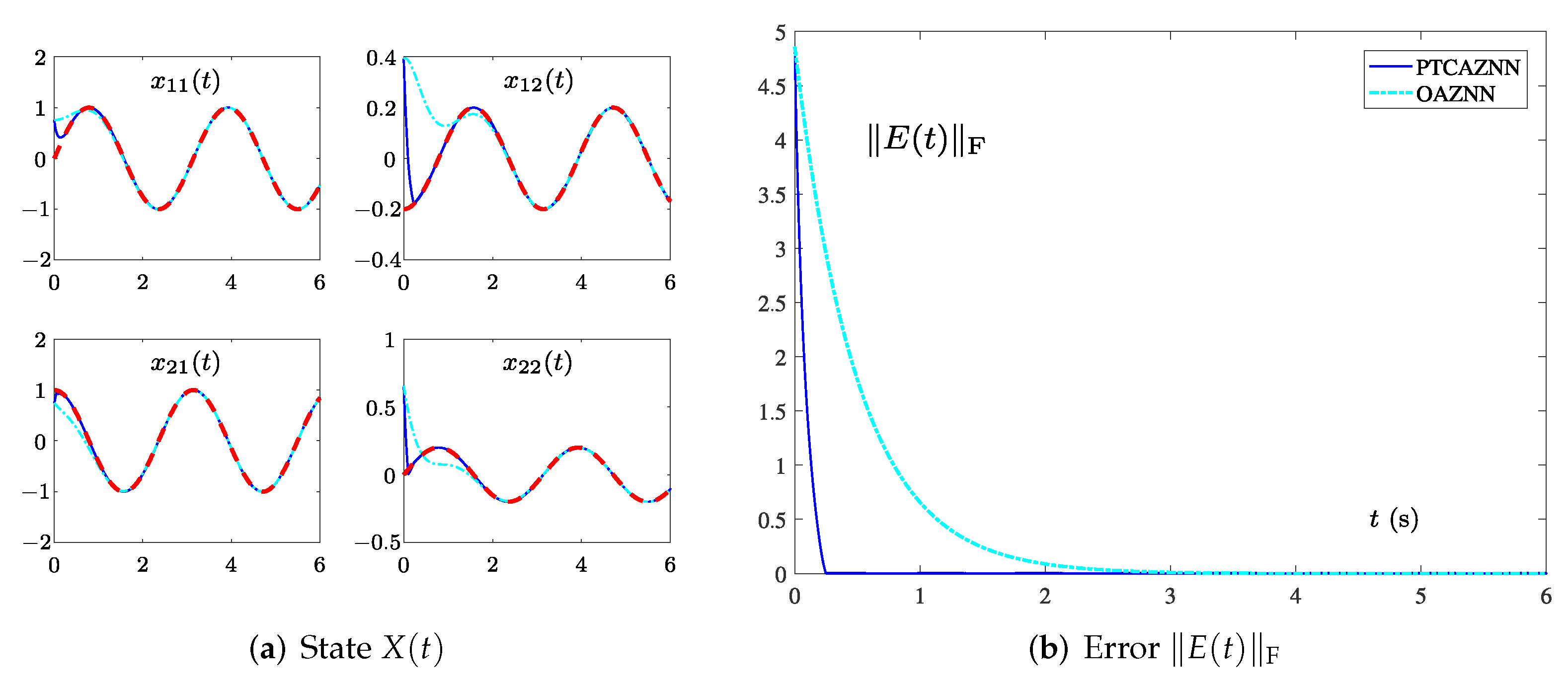
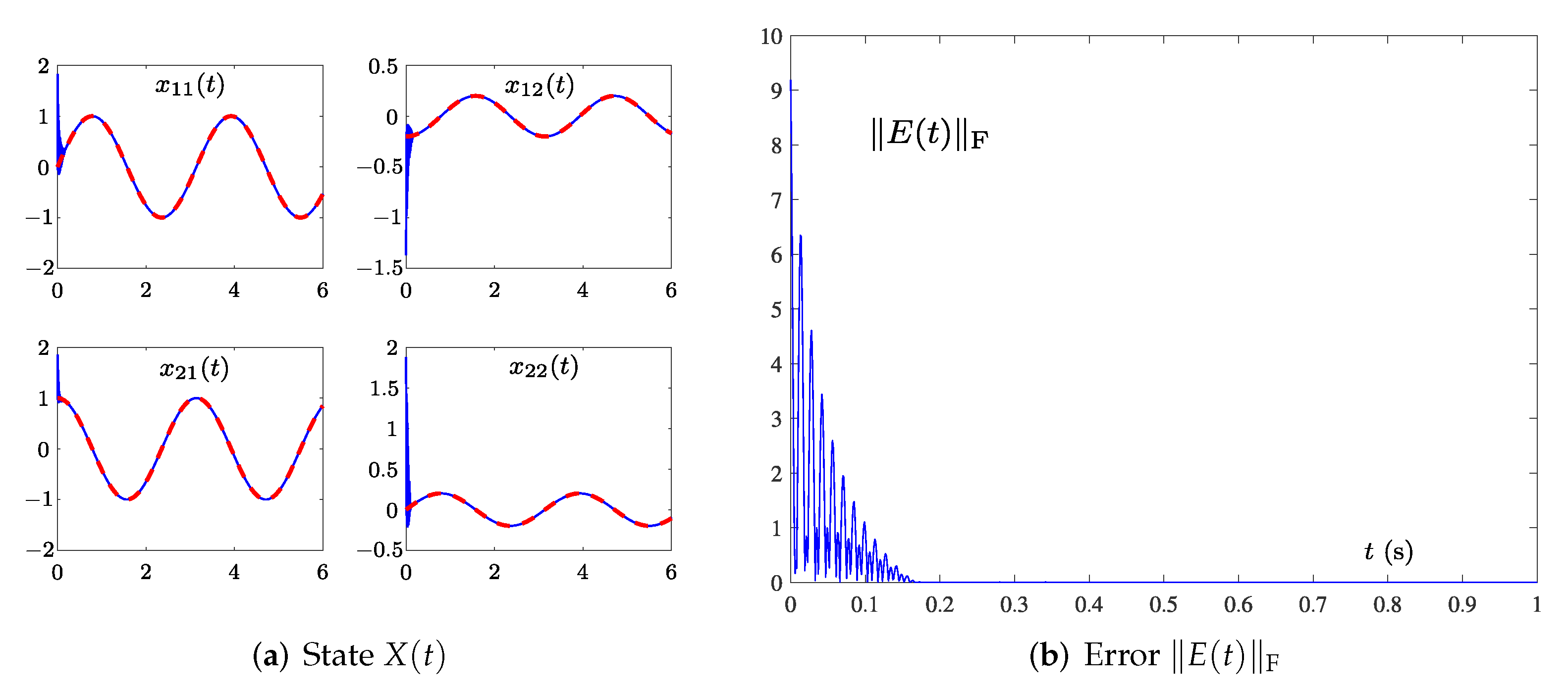
Figure 1a represents the state trajectory of when the and the initial value . The red dotted lines are the ideal trajectory of , the cyan dotted lines and blue lines represent using the OAZNN model (11), and the PTCAZNN model (15) to solve TVMIP of (40), respectively. Compared with the OAZNN model (11), the state trajectory generated by (15) is more consistent with the trajectory of theoretical solution. The predefined convergence time of the PTCAZNN model (15) is calculated as follows without noise according to Inequality (24). In this simulation, we set , , ,
Figure 1b indicates that of (15) converges before 0.3 s, while of (11) converges after about 3.5 s. In Figure 1b, the convergence time of the PTCAZNN model (15) is within the upper bound given by (24), so the simulation results also effectively confirm Theorem 2.
In order to quantitatively illustrate that PTCAZNN model (15) has more excellent convergence performance under the free-noise environment, the following groups of parameters are tested, and the comparison results of specific convergence time are shown in Table 2. When , the corresponding convergence time of OAZNN model (11) is 3.0527 s, 0.7030 s, 0.3161 s, and 0.1275 s, respectively, while the convergence time of the PTCAZNN model (15) is 0.2466 s, 0.1030 s, 0.0265 s, and 0.0105 s. It can be seen that the convergence time of the PTCAZNN model (15) is much faster than the OAZNN model (11). Moreover, the theoretical convergence time of (15) can be calculated as 1 s, 0.2 s, 0.1 s, and 0.04 s, respectively, by Formula (24). Therefore, PTCAZNN (15) can prescribe the convergent time by set parameters for solving TVMIP of (40) in the absence of noise.
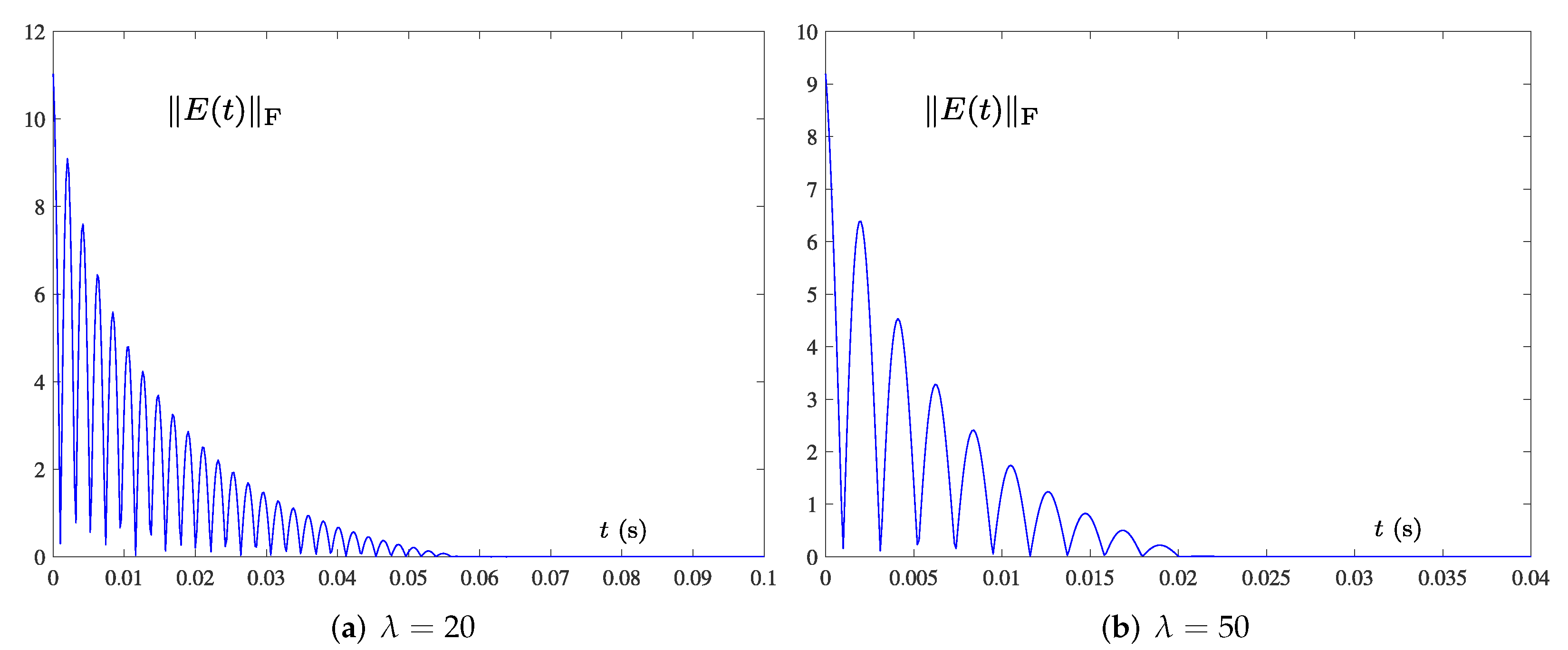
4.2. Single-Harmonic Noise with a Near-Zero Frequency
In fact, the influence of noise can not be ignored, and some noise is likely to lead to the failure of the whole industrial experiment [36]. Thus, the robustness of the model is a key index to appraise the performance of the model. Thus, we take the single-harmonic noises into account in this part. In this simulation examples, the frequency f of single-harmonic noise is close to zero, i.e.,
where the frequency Hz. The homologous results are displayed in Figure 2 and Figure 3. As shown in Figure 2a and Figure 3a, the solid blue lines represent the state trajectory solved by the models, and the dotted red lines are the theoretical solutions. It can be found that model (15) can match the theoretical solution faster than model (11) when solving the TVMIP in the environment of single-harmonic noise.
By comparing Figure 2b and Figure 3b, we realize that solved by OAZNN (11) reaches 0 after about 0.7 s, while in model (15) converges after about 0.047 s. The convergence speed of (15) is about ten times faster than (11). Due to the PTAF (13) used having the ability to reject noises itself and the adaptive term being able to compensate the influence of harmonic noises availably, the PTCAZNN model (15) can realize double noise suppression. It can be concluded that model (15) can suppress noise better than model (11) proposed in previous work [42] under the low frequency single-harmonic noise. The results are the same as expected by previous theoretical results in Section 3.2.
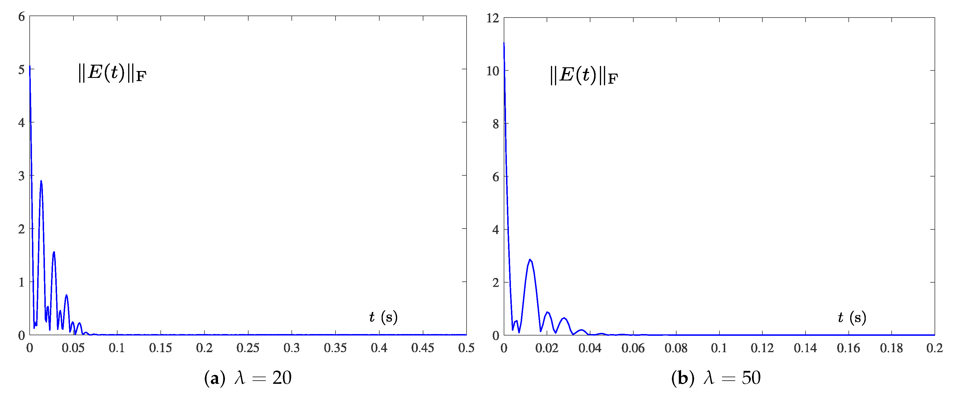
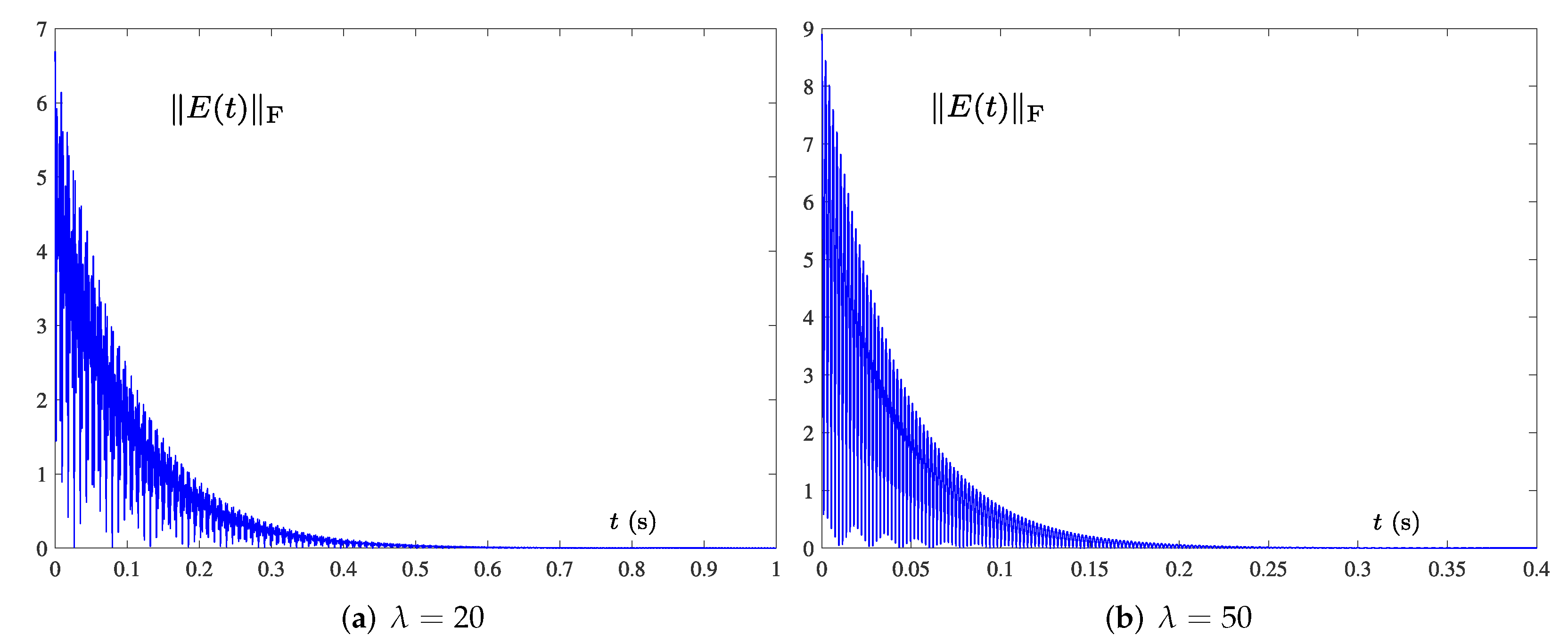
4.3. Single-Harmonic Noise with Nonzero Frequency
In this part, the OAZNN model (11) and PTCAZNN model (15) are tested under the single-harmonic noise with the nonzero frequency as follows:
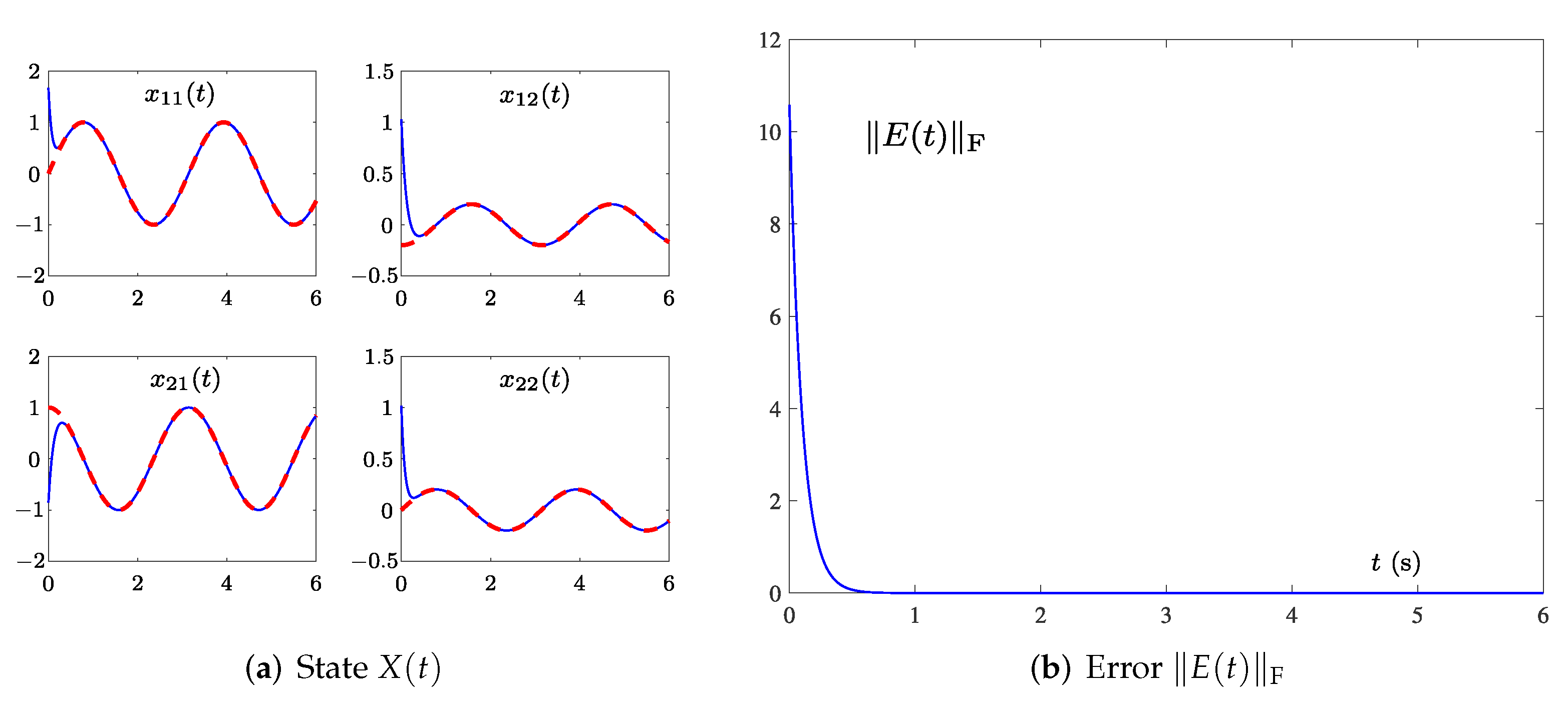
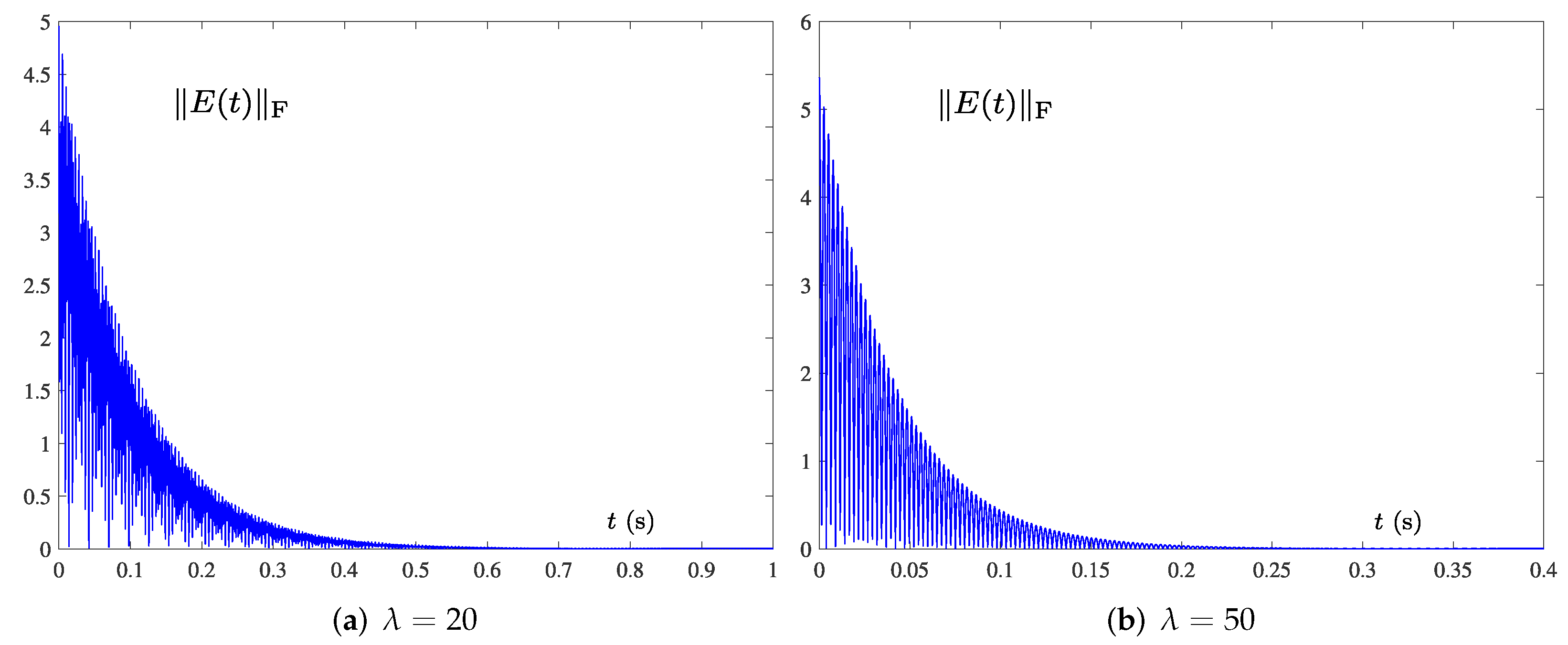
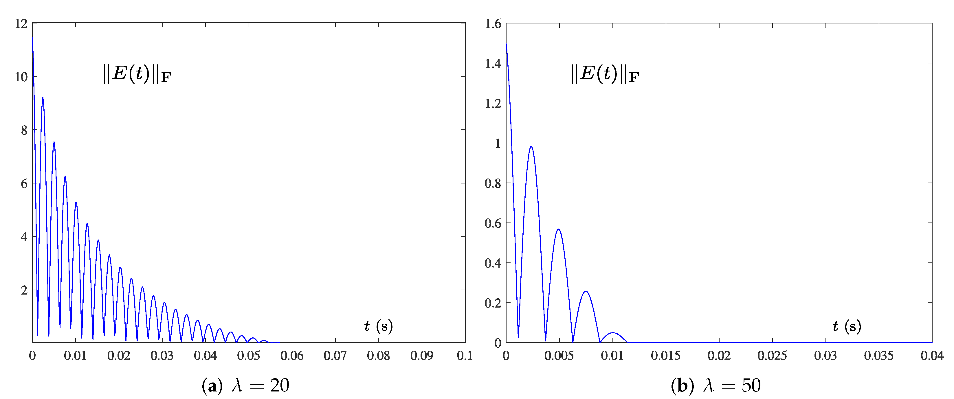
where Hz. The convergence results of state trajectory and of OAZNN (11) and model (15) are shown in Figure 4 and Figure 5, respectively. By comparing Figure 4a and Figure 5a, it is obvious that (11) can fit the trajectory . However, its fitting speed is not as fast as (15). Similarly, the convergence process of in Figure 4b can be completed within 3 s, while the solved by (15) in Figure 5b can converge within 0.2 s. Hence, one can see that the convergence speed of (15) is much faster than that of (11) when Hz. In conclusion, these results confirm the validity and superiority of (15) for TVMIP under the single-harmonic noise with Hz once more.
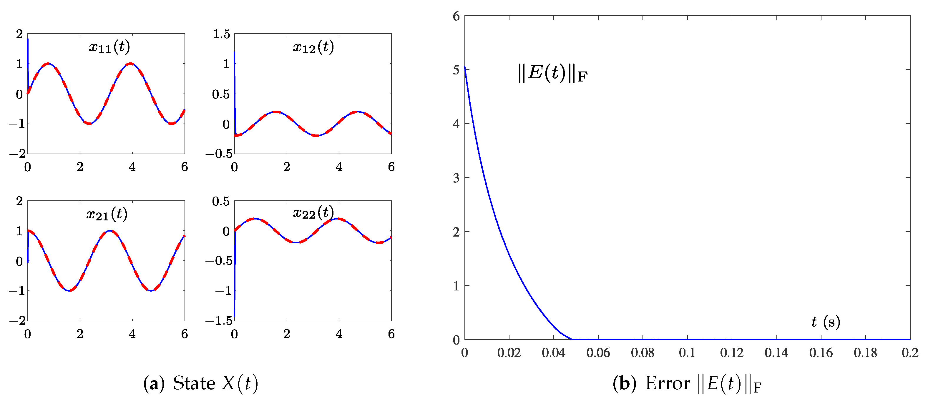
To verify the role of the design parameter in model (15), we observe the performance of the model by varying the design parameter . To be specific, we employ different (i.e., and ) for model (15) in case of Hz. Relevant simulation results are shown in Figure 6, which show that of (15) converges to zero, indicating that the model can successfully solve TVMIP of (40). As illustrated in Figure 6, it is evident that the convergence rate of model (15) can be successfully improved by increasing the in the same frequency Hz.
4.4. Multiple-Harmonic Noises with Periodic and Aperiodic Characteristics
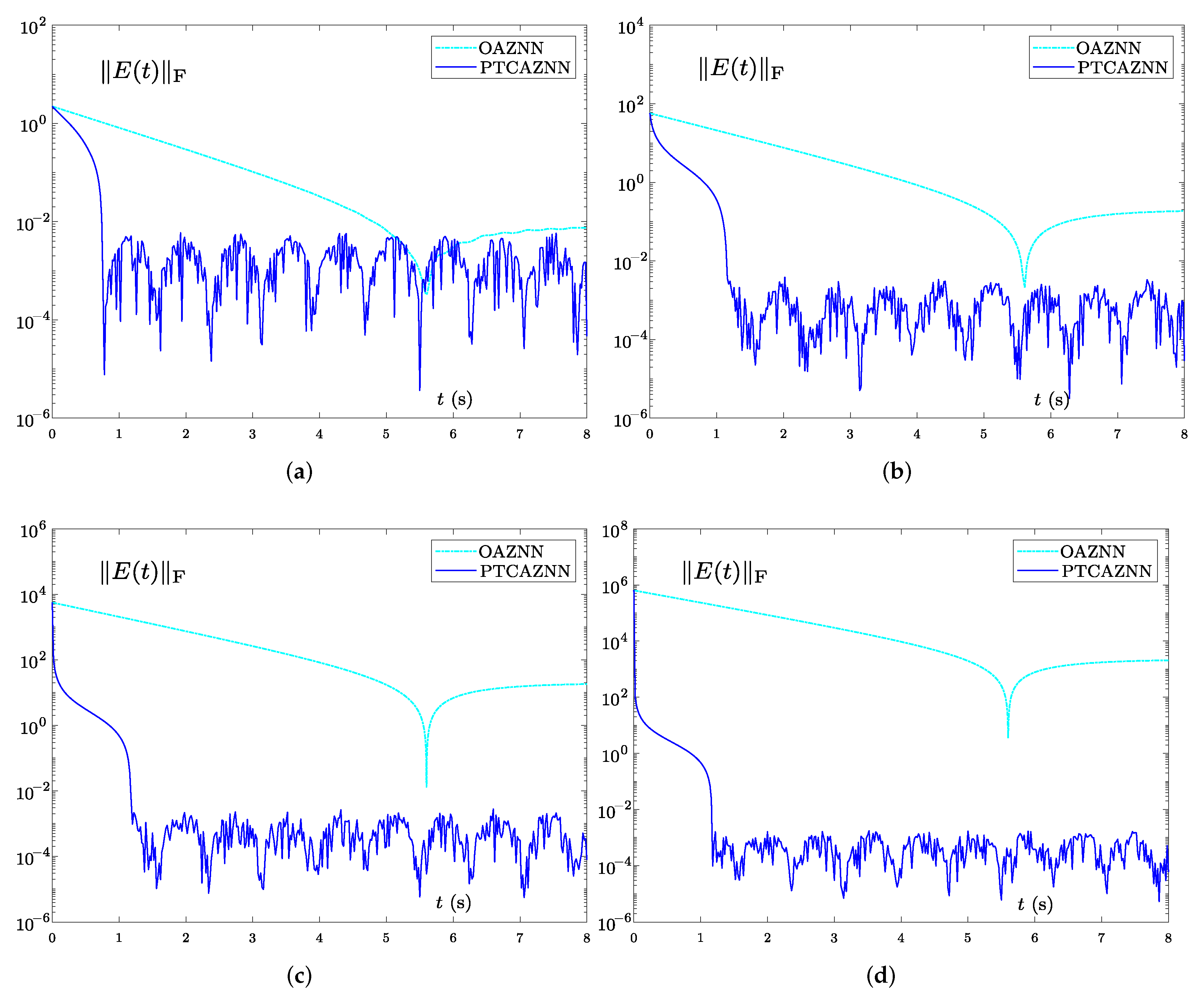
In this subsection, OAZNN (38) and PTCAZNN (39) are conducted to solve TVMIP under multiple-harmonic noises. The following multiple-harmonic noise with periodic period is studied firstly as
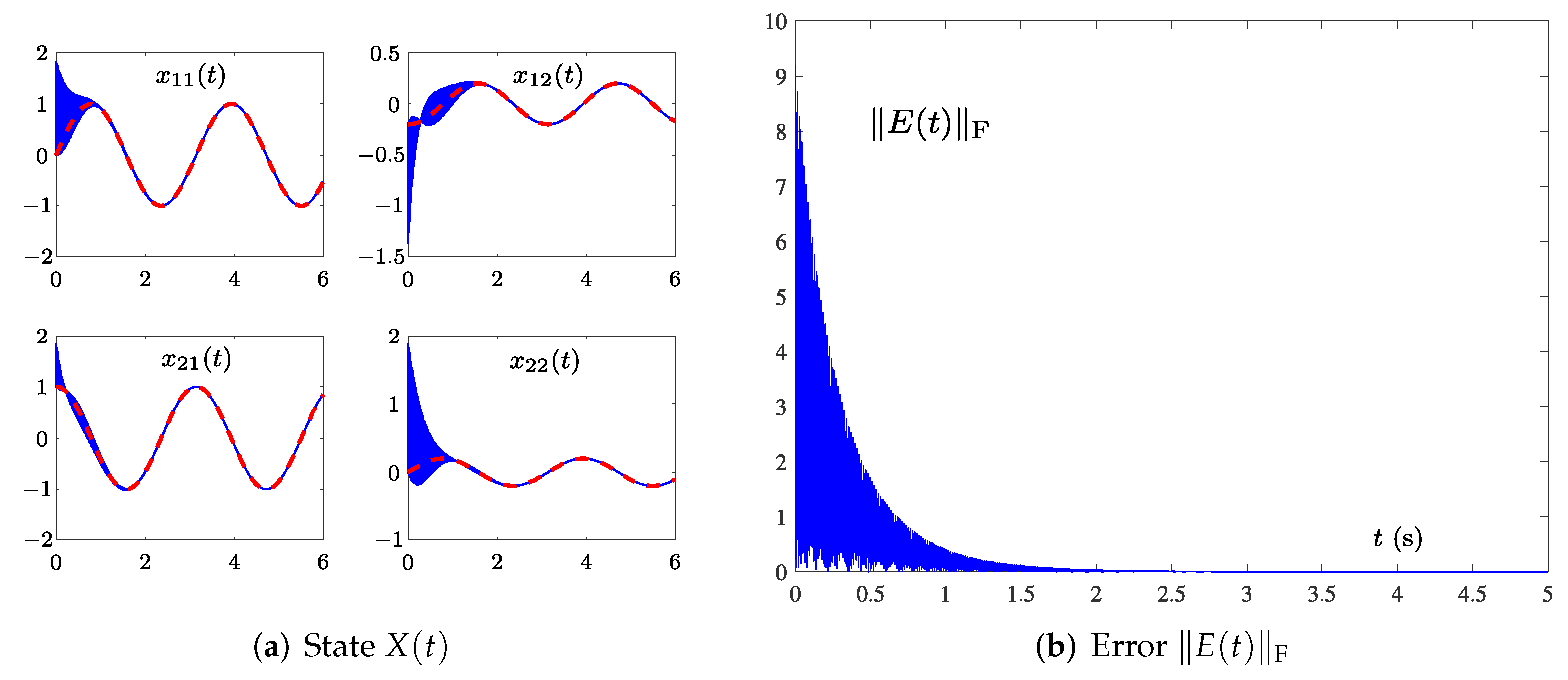
As can be seen from Figure 7 and Figure 8, the synthesized by the OAZNN model (38) and PTCAZNN model (39) can converge to zero, indicating that can converge to the theoretical . However, through comparative observations, it can be found that the convergence speed of (39) is 10 times faster than that of (38) under the same multiple-harmonic noise. For example, when the , model (38) can achieve convergence within 0.6 s, while (39) can achieve convergence within 0.06 s.
The following multiple-harmonic noise with an aperiodic period is used,
Figure 9 and Figure 10 display the corresponding results. Both figures verify that the PTCAZNN model (39) can effectively invert the time-varying matrix considering the interference of multiple-harmonic noises.
To sum up, these comparison results in Figure 8 and Figure 10 confirm the robustness of PTCAZNN model (39) for the TVMIP with multiple harmonic noises. Finally, we summarize the previous simulation results in Table 3 after quantitative analysis. It can be clearly seen that, in various situations (including different frequencies, different periodic characteristics, and different initial states), the PTCAZNN model shows superior convergence performance and robust performance compared to the OAZNN model.
4.5. Sensitivity of Initial Values
As we know, the convergence performance of the existing ZNN is greatly influenced by the initial value. Therefore, it is very necessary to discuss the initial value sensitivity. In this simulation, four random initial values belonging to different intervals are tested, and the results are shown in Figure 11. It is worth noting that we take an error accuracy of as the bound for judging model convergence. The harmonic noise are selected as
As shown in Figure 11a, with , the of the OAZNN model (11) converges in about 5.9 s. In contrast, the of PTCAZNN model (15) converges in 0.78 s. More importantly, as displayed in Figure 11b, with , the of (15) can converge in about 1.12 s, while the of (11) cannot converge. The similar results can be obtained from Figure 11c,d. Table 4 shows a detailed numerical comparison about the upper bound of error of (11) and (15) when the error tends to be stable. When the initial values are in different intervals, the error upper bounds of model (11) are , , , , respectively. Nevertheless, the error upper bounds of model (15) are , , , , respectively. In summary, we can conclude that model (15) is non-sensitive for initial values; however, model (11) may fail for some initial values.
4.6. High-Dimensional Example Verification
Considering another TVMIP with time-varying Toeplitz matrices:
where ; with .
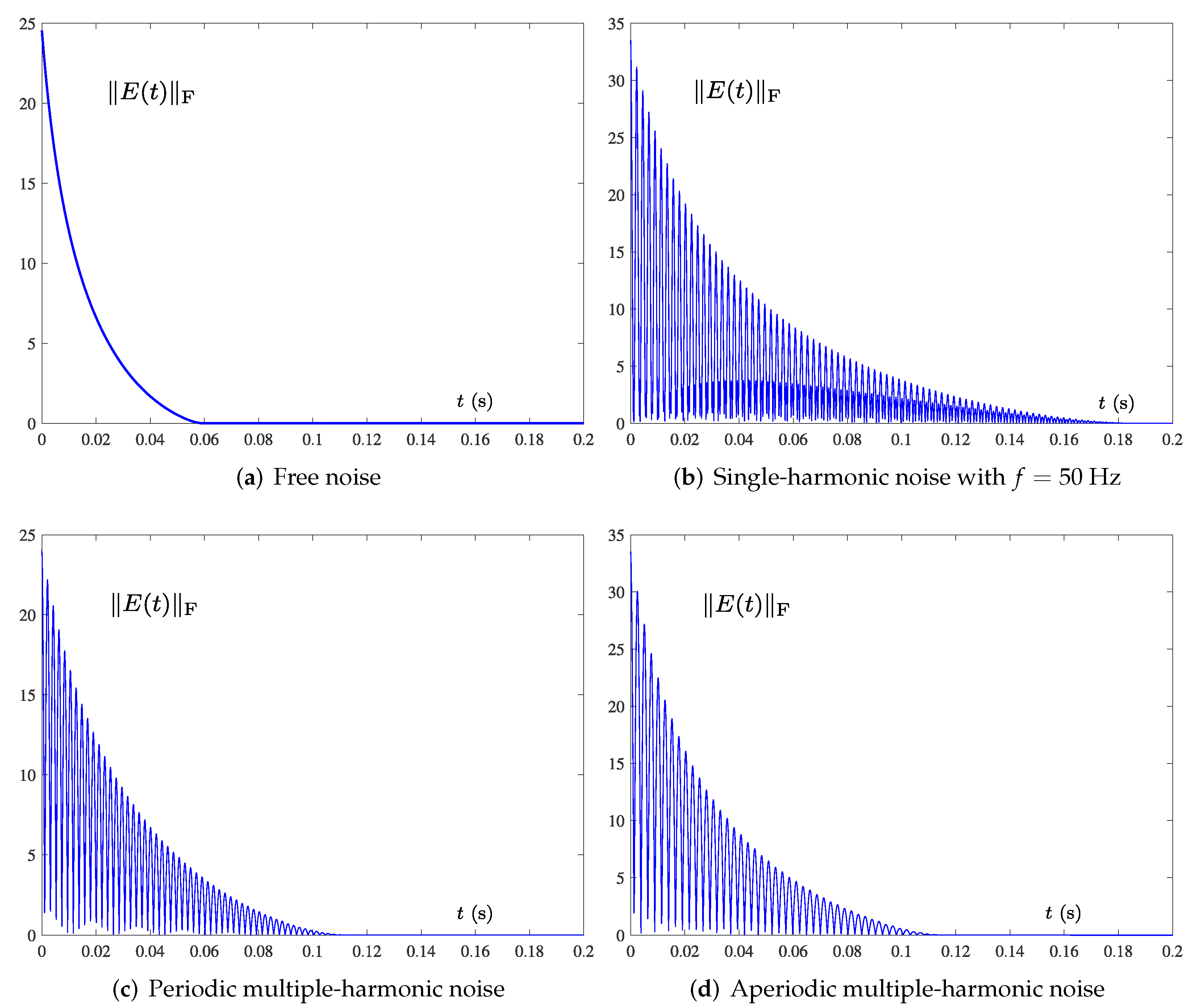
Similarly, in this high-dimensional example simulation, the parameter and other parameters are set in the same way as the previous single harmonic noise. Specifically, it can be seen in Figure 12 that four different cases (no noise in Figure 12a, single harmonic noise with Hz in Figure 12b, periodic multi-harmonic noise in Figure 12c, aperiodic multi-harmonic noise in Figure 12d), the convergence time of model (15) is about 0.06, 0.2, 0.12, 0.12 s. This results are similar to the previous low-dimensional case, indicating that the matrix dimension has little influence on the model solving performance, that is, the PTCAZNN model can maintain satisfactory convergence and robustness even in high dimensions.
5. Conclusions
In this paper, the PTCAZNN model (15) with prescribed-time convergence and double noise suppression has been studied and proposed to resolve the TVMIP. Compared with the OAZNN model (11), this model not only has an adaptive term to compensate and learn noise, but also adds the PTAF to accelerate the convergence rate. In addition, the theoretical analysis of PTCAZNN model (15) with prescribed-time convergence and robustness performance has been provided. Lastly, the simulation results show that model (15) has better convergence performance, anti-interference performance, and lower initial value sensitivity. Thereinto, it can be found that the convergence speed of the PTCAZNN model can be 10 times faster than that of the OAZNN model in some cases.
Author Contributions
Conceptualization, B.L., J.L. and L.H.; methodology, L.H., B.L. and J.L.; software, Y.H.; validation, L.H., X.C. and B.L.; formal analysis, L.H. and X.C.; investigation, Y.H.; data curation, Y.H.; writing—original draft preparation, L.H.; writing—review and editing, B.L. and L.H.; visualization, Y.H.; supervision, B.L. and J.L.; project administration, B.L.; funding acquisition, B.L. All authors have read and agreed to the published version of the manuscript.
Funding
This work was supported in part by the National Natural Science Foundation of China under Grant Nos. 62066015 and 61962023, the Natural Science Foundation of Hunan Province of China under Grant No. 2020JJ4511, and the Research Foundation of Education Bureau of Hunan Province, China, under Grant No. 20A396.
Conflicts of Interest
The authors declare no conflict of interest.
Abbreviations
The following abbreviations are used in this manuscript:
| ZNN | zeroing neural network |
| OAZNN | original adaptive ZNN |
| PTCAZNN | prescribed-time convergent adaptive ZNN |
| GNN | gradient neural network |
| RNN | recurrent neural network |
| AF | activation function |
| PTAF | predefined time AF |
| TVMIP | time-varying matrix inverse problem |
References
- He, Y.; Liao, B.; Xiao, L.; Han, L.; Xiao, X. Double accelerated convergence ZNN with noise-suppression for handling dynamic matrix inversion. Mathematics 2022, 10, 50. [Google Scholar] [CrossRef]
- Liao, B.; Zhang, Y. From different ZFs to different ZNN models accelerated via Li activation functions to finite-time convergence for time-varying matrix pseudoinversion. Neurocomputing 2014, 133, 512–522. [Google Scholar] [CrossRef]
- Liao, B.; Wang, Y.; Li, W.; Peng, C.; Xiang, Q. Prescribed-time convergent and noise-tolerant Z-type neural dynamics for calculating time-dependent quadratic programming. Neural Comput. Applic. 2021, 33, 5327–5337. [Google Scholar] [CrossRef]
- Fan, J.; Jin, L.; Xie, Z.; Li, S.; Zheng, Y. Data-driven motion-force control scheme for redundant manipulators: A kinematic perspective. IEEE Trans. Ind. Inform. 2021, 18, 5338–5347. [Google Scholar] [CrossRef]
- Zhou, P.; Tan, M.; Ji, J.; Jin, J. Design and analysis of anti-noise parameter-variable zeroing neural network for dynamic complex matrix inversion and manipulator trajectory tracking. Electronics 2022, 11, 824. [Google Scholar] [CrossRef]
- Cui, G.; Li, H.; Rangaswamy, M. MIMO radar waveform design with constant modulus and similarity constraints. IEEE Trans. Signal Process. 2013, 62, 343–353. [Google Scholar] [CrossRef]
- Basu, J.K.; Bhattacharyya, D.; Kim, T.h. Use of artificial neural network in pattern recognition. Int. J. Softw. Eng. Its Appl. 2010, 4, 23–34. [Google Scholar]
- Lindfield, G.; Penny, J. Numerical Methods: Using MATLAB; Academic Press: Cambridge, MA, USA, 2018. [Google Scholar]
- Zhang, Y.; Chen, K.; Tan, H.Z. Performance analysis of gradient neural network exploited for online time-varying matrix inversion. IEEE Trans. Autom. Control 2009, 54, 1940–1945. [Google Scholar] [CrossRef]
- Boriskov, P. IoT-oriented design of an associative memory based on impulsive Hopfield neural network with rate coding of LIF oscillators. Electronics 2020, 9, 1468. [Google Scholar] [CrossRef]
- Ramos, H.; Monteiro, M.T.T. A new approach based on the Newton’s method to solve systems of nonlinear equations. J. Comput. Appl. Math. 2017, 318, 3–13. [Google Scholar] [CrossRef]
- Chen, H.C.; Widodo, A.M.; Wisnujati, A.; Rahaman, M.; Lin, J.C.W.; Chen, L.; Weng, C.E. AlexNet convolutional neural network for disease detection and classification of tomato leaf. Electronics 2022, 11, 951. [Google Scholar] [CrossRef]
- Webber, J.; Mehbodniya, A.; Teng, R.; Arafa, A. Human–Machine interaction using probabilistic neural network for light communication systems. Electronics 2022, 11, 932. [Google Scholar] [CrossRef]
- Stanimirović, P.S.; Petković, M.D. Gradient neural dynamics for solving matrix equations and their applications. Neurocomputing 2018, 306, 200–212. [Google Scholar] [CrossRef]
- Zhang, B.; Liu, Y.; Cao, J.; Wu, S.; Wang, J. Fully complex conjugate gradient-based neural networks using wirtinger calculus framework: Deterministic convergence and its application. Neural Netw. 2019, 115, 50–64. [Google Scholar] [CrossRef]
- Zhang, Y.; Guo, D.; Li, Z. Common nature of learning between back-propagation and hopfield-type neural networks for generalized matrix inversion with simplified models. IEEE Trans. Neural Netw. Learn. Syst. 2013, 24, 579–592. [Google Scholar] [CrossRef]
- Zhang, Y.; Li, Z. Zhang neural network for online solution of time-varying convex quadratic program subject to time-varying linear-equality constraints. Phys. Lett. A 2009, 373, 1639–1643. [Google Scholar] [CrossRef]
- Guo, D.; Zhang, Y. Zhang neural network, Getz–Marsden dynamic system, and discrete-time algorithms for time-varying matrix inversion with application to robots’ kinematic control. Neurocomputing 2012, 97, 22–32. [Google Scholar] [CrossRef]
- Li, W. A recurrent neural network with explicitly definable convergence time for solving time-variant linear matrix equations. IEEE Trans. Ind. Inform. 2018, 14, 5289–5298. [Google Scholar] [CrossRef]
- Xiao, L. A new design formula exploited for accelerating Zhang neural network and its application to time-varying matrix inversion. Theor. Comput. Sci. 2016, 647, 50–58. [Google Scholar] [CrossRef]
- Jin, L.; Zhang, Y. Discrete-time Zhang neural network for online time-varying nonlinear optimization with application to manipulator motion generation. IEEE Trans. Neural Netw. Learn. Syst. 2014, 26, 1525–1531. [Google Scholar]
- Xiao, L.; Liao, B.; Li, S.; Zhang, Z.; Ding, L.; Jin, L. Design and analysis of FTZNN applied to the real-time solution of a nonstationary Lyapunov equation and tracking control of a wheeled mobile manipulator. IEEE Trans. Ind. Inform. 2017, 14, 98–105. [Google Scholar] [CrossRef]
- Zhang, Y.; Qi, Z.; Qiu, B.; Yang, M.; Xiao, M. Zeroing neural dynamics and models for various time-varying problems solving with ZLSF models as minimization-type and euler-type special cases [Research Frontier]. IEEE Comput. Intell. Mag. 2019, 14, 52–60. [Google Scholar] [CrossRef]
- Jin, L.; Li, S.; Liao, B.; Zhang, Z. Zeroing neural networks: A survey. Neurocomputing 2017, 267, 597–604. [Google Scholar] [CrossRef]
- Liao, B.; Xiao, L.; Jin, J.; Ding, L.; Liu, M. Novel complex-valued neural network for dynamic complex-valued matrix inversion. J. Adv. Comput. Intell. Intell. Inform. 2016, 20, 132–138. [Google Scholar] [CrossRef]
- Sun, C.; Gao, H.; He, W.; Yu, Y. Fuzzy neural network control of a flexible robotic manipulator using assumed mode method. IEEE Trans. Neural Netw. Learn. Syst. 2018, 29, 5214–5227. [Google Scholar] [CrossRef]
- Yañez-Badillo, H.; Beltran-Carbajal, F.; Tapia-Olvera, R.; Favela-Contreras, A.; Sotelo, C.; Sotelo, D. Adaptive robust motion control of quadrotor systems using artificial neural networks and particle swarm optimization. Mathematics 2021, 9, 2367. [Google Scholar] [CrossRef]
- Jin, L.; Li, S.; Xiao, L.; Lu, R.; Liao, B. Cooperative motion generation in a distributed network of redundant robot manipulators with noises. IEEE Trans. Syst. Man Cybern. Syst. 2017, 48, 1715–1724. [Google Scholar] [CrossRef]
- Liao, B.; Zhang, Y.; Jin, L. Taylor O(h3) discretization of ZNN models for dynamic equality-constrained quadratic programming with application to manipulators. IEEE Trans. Neural Netw. Learn. Syst. 2015, 27, 225–237. [Google Scholar] [CrossRef]
- Wei, Q.; Li, H.; Yang, X.; He, H. Continuous-time distributed policy iteration for multicontroller nonlinear systems. IEEE Trans. Cybern. 2020, 51, 2372–2383. [Google Scholar] [CrossRef]
- Liu, M.; Chen, L.; Du, X.; Jin, L.; Shang, M. Activated gradients for deep neural networks. IEEE Trans. Neural Netw. Learn. Syst. 2021. [Google Scholar] [CrossRef]
- Hu, Z.; Xiao, L.; Li, K.; Li, K.; Li, J. Performance analysis of nonlinear activated zeroing neural networks for time-varying matrix pseudoinversion with application. Appl. Soft Comput. 2021, 98, 106735. [Google Scholar] [CrossRef]
- Li, W.; Liao, B.; Xiao, L.; Lu, R. A recurrent neural network with predefined-time convergence and improved noise tolerance for dynamic matrix square root finding. Neurocomputing 2019, 337, 262–273. [Google Scholar] [CrossRef]
- Jin, L.; Zhang, Y.; Li, S. Integration-enhanced Zhang neural network for real-time-varying matrix inversion in the presence of various kinds of noises. IEEE Trans. Neural Netw. Learn. Syst. 2015, 27, 2615–2627. [Google Scholar] [CrossRef] [PubMed]
- Benedetto, J.J. Harmonic Analysis and Applications; CRC Press: Boca Raton, FL, USA, 2020. [Google Scholar]
- Karslı, H.; Dondurur, D. A mean-based filter to remove power line harmonic noise from seismic reflection data. J. Appl. Geophys. 2018, 153, 90–99. [Google Scholar] [CrossRef]
- Taghia, J.; Martin, R. A frequency-domain adaptive line enhancer with step-size control based on mutual information for harmonic noise reduction. IEEE/ACM Trans. Audio Speech Lang. Process. 2016, 24, 1140–1154. [Google Scholar] [CrossRef]
- Mo, Z.; Wang, J.; Zhang, H.; Miao, Q. Weighted cyclic harmonic-to-noise ratio for rolling element bearing fault diagnosis. IEEE Trans. Instrum. Meas. 2019, 69, 432–442. [Google Scholar] [CrossRef]
- Oppenheim, A.V.; Willsky, A.S.; Nawab, S.H.; Hernández, G.M.; Fernández, A.S. Signals & Systems; Pearson Educación: New York, NJ, USA, 1997. [Google Scholar]
- Jacob, B.; Baiju, M. Space-vector-quantized dithered sigma–delta modulator for reducing the harmonic noise in multilevel converters. IEEE Trans. Ind. Electron. 2014, 62, 2064–2072. [Google Scholar] [CrossRef]
- Li, S.; Zhou, M.; Luo, X. Modified primal-dual neural networks for motion control of redundant manipulators with dynamic rejection of harmonic noises. IEEE Trans. Neural Netw. Learn. Syst. 2017, 29, 4791–4801. [Google Scholar] [CrossRef]
- Guo, D.; Li, S.; Stanimirović, P.S. Analysis and application of modified ZNN design with robustness against harmonic noise. IEEE Trans. Ind. Inform. 2019, 16, 4627–4638. [Google Scholar] [CrossRef]
Figure 1.
Simulation results by the OAZNN model (11) and PTCAZNN model (15) with for TVMIP of (40) in the absence of noise.

Figure 2.
Simulation results by the OAZNN model (11) with for TVMIP of (40) under the same single-harmonic noise when Hz.

Figure 3.
Simulation results by the PTCAZNN model (15) with for TVMIP of (40) under the same single-harmonic noise when Hz.

Figure 4.
Simulation results by the OAZNN model (11) with for TVMIP of (40) under the same single-harmonic noise when Hz.

Figure 5.
Simulation results by the PTCAZNN model (15) with for TVMIP of (40) under the same single-harmonic noise when Hz.

Figure 6.
Simulation results by the PTCAZNN model (15) with for TVMIP of (40) under the same single-harmonic noise when Hz.

Figure 7.
Simulation results under the constant periodic multiple-harmonic noise, OAZNN model (38) for TVMIP of (40) with , respectively.

Figure 8.
Simulation results under the constant periodic multiple-harmonic noise, the PTCAZNN model (39) for TVMIP of (40) with respectively.

Figure 9.
Simulation results under the aperiodic multiple-harmonic noise, OAZNN model (38) for TVMIP of (40) with respectively.

Figure 10.
Simulation results under the aperiodic multiple-harmonic noise, PTCAZNN model (39) for TVMIP of (40) with , respectively.

Figure 11.
Dynamic characteristics of OAZNN (11) and PTCAZNN (15) when and . With (a) ; (b) ; (c) ; (d) .

Figure 12.
Dynamic characteristics of PTCAZNN (15) for high-dimensional matrix inversion under various noise.
Figure 12.
Dynamic characteristics of PTCAZNN (15) for high-dimensional matrix inversion under various noise.


| Model | OAZNN Model | PTCAZNN Model |
|---|---|---|
| Design Formula | ||
| Convergence | exponential convergence | predefined-time convergence |
| Robustness | strong | stronger |
| Initial sensitivity | high | low |
Table 2.
Convergence time (CT) of the OAZNN model and PTCAZNN model in the absence of noise (the convergence accuracy is ).
Table 2.
Convergence time (CT) of the OAZNN model and PTCAZNN model in the absence of noise (the convergence accuracy is ).
| Parameter | OAZNN Model | PTCAZNN Model | |
|---|---|---|---|
| Practical CT | Theoretical Computing CT | ||
| 3.0527 s | 0.2466 s | 1 s | |
| 0.7030 s | 0.1030 s | 0.2 s | |
| 0.3161 s | 0.0265 s | 0.1 s | |
| 0.1275 s | 0.0105 s | 0.04 s | |
Table 3.
Convergence time of the OAZNN model and PTCAZNN model using the same parameters under different noise conditions (the convergence accuracy is ).
Table 3.
Convergence time of the OAZNN model and PTCAZNN model using the same parameters under different noise conditions (the convergence accuracy is ).
| Noise | OAZNN Model | PTCAZNN Model |
|---|---|---|
| Near-zero frequency (42) | 0.6950 s | 0.0480 s |
| Nonzero frequency (43) | 2.4470 s | 0.1730 s |
| Periodic (44) | 0.6672 s | 0.0568 s |
| Aperiodic (45) | 0.5980 s | 0.0688 s |
Table 4.
Upper bound of error of the OAZNN model and PTCAZNN model at different initial values.
| Initial Value | OAZNN Model | PTCAZNN Model |
|---|---|---|
Publisher’s Note: MDPI stays neutral with regard to jurisdictional claims in published maps and institutional affiliations. |
© 2022 by the authors. Licensee MDPI, Basel, Switzerland. This article is an open access article distributed under the terms and conditions of the Creative Commons Attribution (CC BY) license (https://creativecommons.org/licenses/by/4.0/).
Share and Cite
MDPI and ACS Style
Liao, B.; Han, L.; He, Y.; Cao, X.; Li, J. Prescribed-Time Convergent Adaptive ZNN for Time-Varying Matrix Inversion under Harmonic Noise. Electronics 2022, 11, 1636. https://0-doi-org.brum.beds.ac.uk/10.3390/electronics11101636
AMA Style
Liao B, Han L, He Y, Cao X, Li J. Prescribed-Time Convergent Adaptive ZNN for Time-Varying Matrix Inversion under Harmonic Noise. Electronics. 2022; 11(10):1636. https://0-doi-org.brum.beds.ac.uk/10.3390/electronics11101636
Chicago/Turabian StyleLiao, Bolin, Luyang Han, Yongjun He, Xinwei Cao, and Jianfeng Li. 2022. "Prescribed-Time Convergent Adaptive ZNN for Time-Varying Matrix Inversion under Harmonic Noise" Electronics 11, no. 10: 1636. https://0-doi-org.brum.beds.ac.uk/10.3390/electronics11101636
Note that from the first issue of 2016, this journal uses article numbers instead of page numbers. See further details here.