
Graph-Embedded Online Learning for Cell Detection and Tumour Proportion Score Estimation


1
School of Computer Science and Technology, Donghua University, Shanghai 201600, China
2
Shanghai Key Laboratory of Multidimensional Information Processing, East China Normal University, Shanghai 200241, China
*
Author to whom correspondence should be addressed.
Electronics 2022, 11(10), 1642; https://0-doi-org.brum.beds.ac.uk/10.3390/electronics11101642
Submission received: 10 April 2022
/
Revised: 13 May 2022
/
Accepted: 15 May 2022
/
Published: 21 May 2022
(This article belongs to the Special Issue Deep Learning for Big Data Processing)
Abstract
:Cell detection in microscopy images can provide useful clinical information. Most methods based on deep learning for cell detection are fully supervised. Without enough labelled samples, the accuracy of these methods would drop rapidly. To handle limited annotations and massive unlabelled data, semi-supervised learning methods have been developed. However, many of these are trained off-line, and are unable to process new incoming data to meet the needs of clinical diagnosis. Therefore, we propose a novel graph-embedded online learning network (GeoNet) for cell detection. It can locate and classify cells with dot annotations, saving considerable manpower. Trained by both historical data and reliable new samples, the online network can predict nuclear locations for upcoming new images while being optimized. To be more easily adapted to open data, it engages dynamic graph regularization and learns the inherent nonlinear structures of cells. Moreover, GeoNet can be applied to downstream tasks such as quantitative estimation of tumour proportion score (TPS), which is a useful indicator for lung squamous cell carcinoma treatment and prognostics. Experimental results for five large datasets with great variability in cell type and morphology validate the effectiveness and generalizability of the proposed method. For the lung squamous cell carcinoma (LUSC) dataset, the detection F1-scores of GeoNet for negative and positive tumour cells are 0.734 and 0.769, respectively, and the relative error of GeoNet for TPS estimation is 11.1%.
1. Introduction
Cell detection can be regarded as a combination of nuclear localization and cell classification. It can provide useful clinical information about the cells of interest, such as the presence of cancer cells in a microscopy image [1]. To realize automatic detection and achieve high accuracy, a number of cell localization and classification methods based on machine learning have been proposed. Recently, deep learning has further increased the accuracy of these methods, thanks to its feature representation ability [2]. However, most of these methods are trained in a fully supervised manner, the success of which is highly dependent on precisely labelled samples. Some methods even require datasets with cell contours or masks [3,4,5,6]. Meanwhile, it is difficult to obtain large sets of precise labels at low cost, as cell annotation consumes lots of time and human effort. Thus, semi-supervised methods have been proposed to address the problem [7,8]. These are designed to increase representation power and save annotation efforts, by exploiting patterns in labelled and unlabelled data sets. But many of them are trained off-line, and unable to deal with new images which are constantly generated in pathology labs and may contain variable unseen patterns. Moreover, networks designed for multiple tasks including localization and classification usually take complicated forms, reducing their practicability and limiting their application.
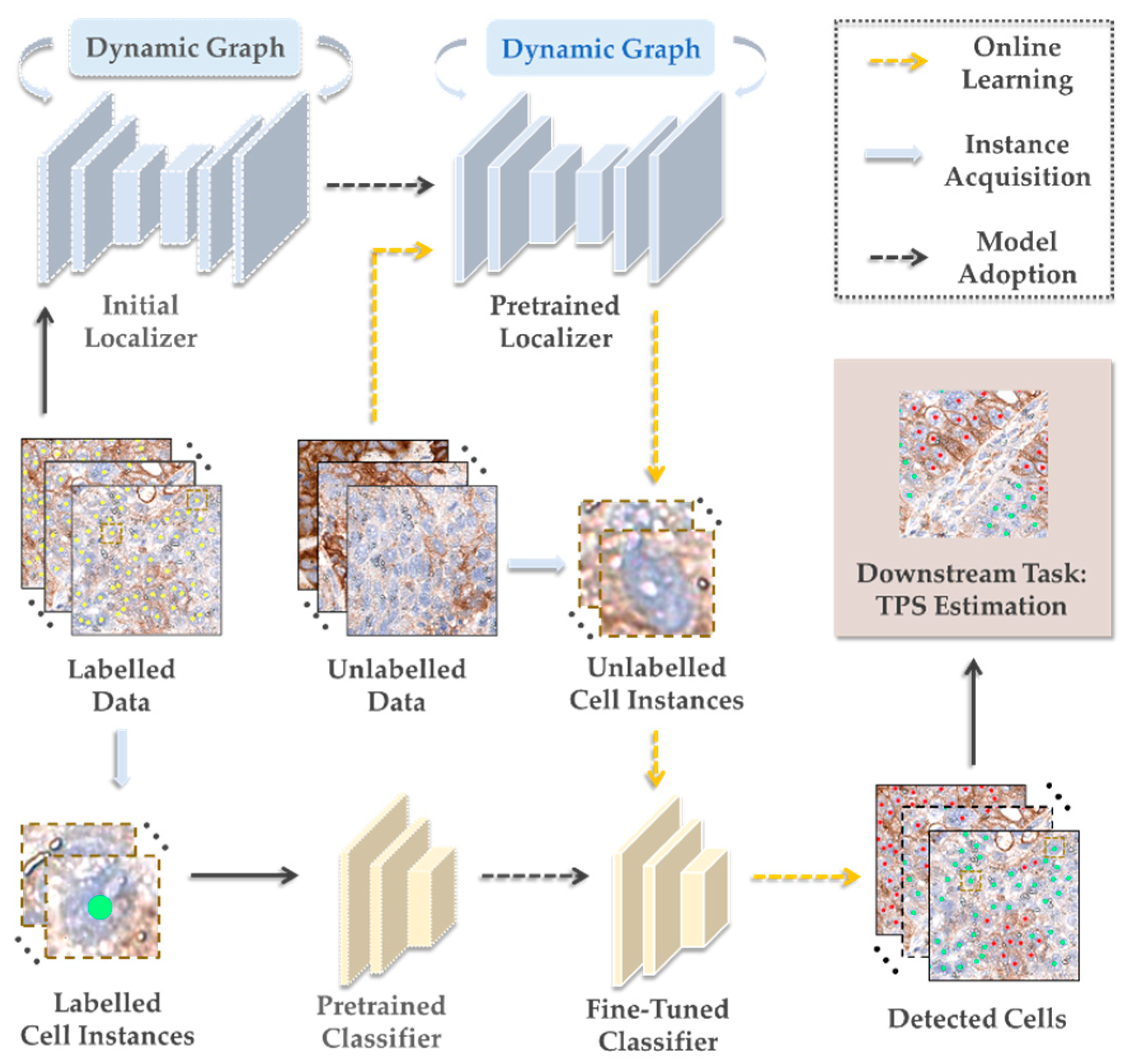
Therefore, we propose a graph-embedded online learning network (GeoNet) for cell detection. GeoNet consists of two modules, one for localization and the other for classification. It generates distance maps [1] with dot annotations roughly indicating locations of nuclei in historical images, as illustrated by Figure 1. It uses an encoder-decoder with dynamic graph embedding for distance map regression and online nuclear localization. It then obtains from new images cell instances with the predicted nuclear locations and classifies them using a pretrained network. The main contributions of this work are as follows:
- It proposes an online learning network, GeoNet, for cell detection in open datasets. It is trained in a semi-supervised fashion, which enables learning features from unknown images while simultaneously predicting nuclear locations. It uses incomplete annotations and saves manual effort. To avoid introducing errors, GeoNet selects only the most reliable new samples with rigid confidence measured according to morphology features of extracted nuclear instances to optimize the backbone.
- The proposed GeoNet is designed to adapt to new images with various cell patterns. It leverages historical data and new images to enhance its feature representation ability and increase nuclear localization accuracy. Moreover, it engages dynamic graph regularization and learns inherent nonlinear structures of cells to gain generalizability.
- GeoNet is a practical solution for computer-aided biomedical study and pathology diagnosis. It is a flexible framework, allowing any encoder-decoders for regression or pretrained networks for classification. Moreover, the cell detection results it produces can easily be used in many downstream applications, such as estimation of tumour proportion score (TPS), which is a key measurement for prognosis and treatment of lung squamous cell carcinoma (LUSC) [9].
In this paper we validate the efficacy of GeoNet using five large datasets with great variability in cell type and morphology. We demonstrate how it can be applied to a downstream task, TPS estimation, using Programmed Death Ligand 1 (PD-L1) slides of LUSC, obtained from first-hand clinical data.
2. Related Works
There are three main ways to detect cells in microscopy images, placing bounding boxes around cells [8], drawing cell contours or masks [3,4,5,6], and looking for nuclei [1,10,11,12,13]. Some cell detection methods combine localization and classification [3,12,14,15,16], while others perform only localization [10,11,17,18,19].
Methods that combine localization and classification can be categorized into multi-stage and end-to-end methods. Multi-stage methods usually extract cell masks and then classify cells. Theera-Umpon et al. [20] applied a fuzzy C-means (FCM) algorithm to locate cells and neural networks to classify cells. Sharma et al. [21] used a contour-based minimum-model to locate cells and AdaBoost to realize classification. Multi-stage methods are intuitive and their requirements for cell location labels are low. However, their final outcome relies on the output of each intermediate step. End-to-end methods can simultaneously locate and classify cells. Graham et al. [3] proposed a Horizontal-Vertical-Network (HoVer-Net) using horizontal and vertical maps to separate occluded or overlapping cells, with multi-branch architecture to realize cell segmentation and classification concurrently. In this kind of method, cell classification is not dependent on localization. However, these techniques require large amounts of precisely labelled data and their models are complex.
Methods that only locate cells can be grouped into conventional machine learning methods and deep learning methods. In the first group, watershed algorithms are usually employed for cell feature extraction [22,23]. The watershed algorithm requires less computation than deep networks, and is thus more efficient. However, it relies on predefined geometry of nuclei, which limits its accuracy and generalizability as nuclear patterns may vary greatly. Deep learning methods can represent nuclear features with better generalizability. Chen et al. [10] use U-Net as the backbone and direction field map as the regression target to deal with overlapping and occluded cells. Deep learning methods reach higher accuracy than conventional methods of cell localization. However, most of the existing deep learning methods do not consider previously unseen patterns in open data, which limits their applications.
From the perspective of supervision, cell detection methods can be categorized as unsupervised, supervised and semi-supervised. Unsupervised methods locate cells by means of scale-invariant morphological feature extraction and clustering, without the need for annotations [24,25]. These methods are efficient, but their overall performance is poor because they lack the guidance of prior learning. Supervised methods can accurately detect cells when trained by abundant labelled data. Xie et al. [1] used a fully residual convolutional neural network to locate nuclei by regressing distance maps. Tofighi et al. [26] used cell shape as prior knowledge to construct regularization and improve accuracy. However, supervised methods depend highly on labelled data, some methods requiring prior domain knowledge or precise labels such as contours, costing considerable human workload. Semi-supervised detection models are trained on both labelled and unlabelled data. Unlike their supervised counterparts, they can utilize partially annotated datasets. Ying et al. [8] manually filtered prediction results to re-train the network. Li et al. [7] proposed self-training to handle incomplete annotations and applied cooperative training to process unlabelled samples. However, existing semi-supervised methods lack the adaptive ability to learn patterns from unknown data.
The results of cell detection can be used for downstream tasks such as TPS estimation [27,28] and HER2 scoring [15]. To date, TPS estimation using pathology image analysis for cancer diagnosis and prognostics has not been intensively studied. TPS refers to the proportion of positive tumour cells in the total number of surviving tumour cells. Some methods have been proposed [27] for TPS estimation, but they usually depend on large complex networks to yield accurate results.
3. Methods
3.1. The Whole Pipeline for Online Cell Detection
To address the issues with existing cell detection methods, we propose GeoNet as illustrated by Figure 2. It contains two modules, nuclear localization and cell classification. The former is a semi-supervised regression network consisting of an encoder-decoder as the backbone and a dynamic graph regularizer, responsible for robust feature representation and distance map prediction. It enables GeoNet to infer nuclear locations from the predicted distance maps for new data examples encountered during training, while being optimized with historical and new samples. The latter adopts a pretrained network to classify the cell instances drawn from the predicted locations. The detection results yielded by GeoNet can be leveraged in many downstream tasks, for example, TPS estimation. Let a microscopy image be denoted by , where and , , and stand for height, width, number of channels and number of images, respectively. Here, . As manual annotations, holds locations (i.e., row and column indexes) of dots on nuclei and contains classes of cells, where and is number of cells in and is number of classes in all the available data examples. Given the input image , GeoNet predicts its nuclear locations and cell types . The details of the proposed network are introduced as follows.
3.2. Nuclear Localization
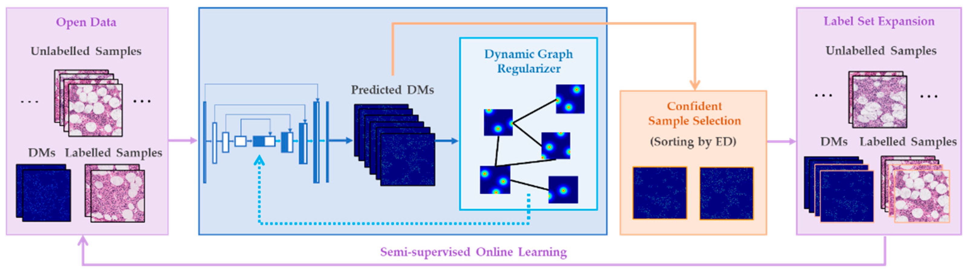
The nuclear localizer in GeoNet is primarily a semi-supervised regression network regularized by dynamic graphs, as illustrated by Figure 3. Apart from the backbone, it also involves necessary preprocessing and postprocessing techniques.
3.2.1. Preprocessing
- (1)
- Patch split: To increase detection accuracy and reduce computational cost in each epoch, the microscopy images are split in an open dataset into patches , where , and represent the numbers of historical samples with dot annotations on nuclei and newly collected samples without any labels, respectively.
- (2)
- Distance map generation: Distance maps are used instead of location coordinates to train a regression network for cell detection, because the distance maps not only reflect nuclear locations but also encode spatial and morphological information of cells. The distance maps provide a better optimization goal for feature representation. They are also useful for confidence measurement and reliable sample selection, which is the key to our semi-supervised mechanism, to be fully introduced in the next subsection.
Given a labelled patch () with cells inside, its dot annotations are transformed to vectorized distance map [1] with
where , represents the shortest spatial Euclidean distance (ED) between the th pixel and an annotation, and is a constant set by users.
3.2.2. Graph-Embedded Network for Semi-Supervised Regression
After preprocessing, the patches are fed into the proposed graph-embedded regression network for nuclear localization. As illustrated by Figure 3, the network is semi-supervised, first pretrained on the labelled data and then fine-tuned by both labelled and unlabelled data , where is the predicted distance map. The network gains the basic ability to recognize cell patterns in pretraining, while adapting to new images during fine-tuning and becoming capable of detecting crowded cells online.
The backbone of the localization network is denoted by , where represents learnable parameters. It regresses the distance maps with the following loss
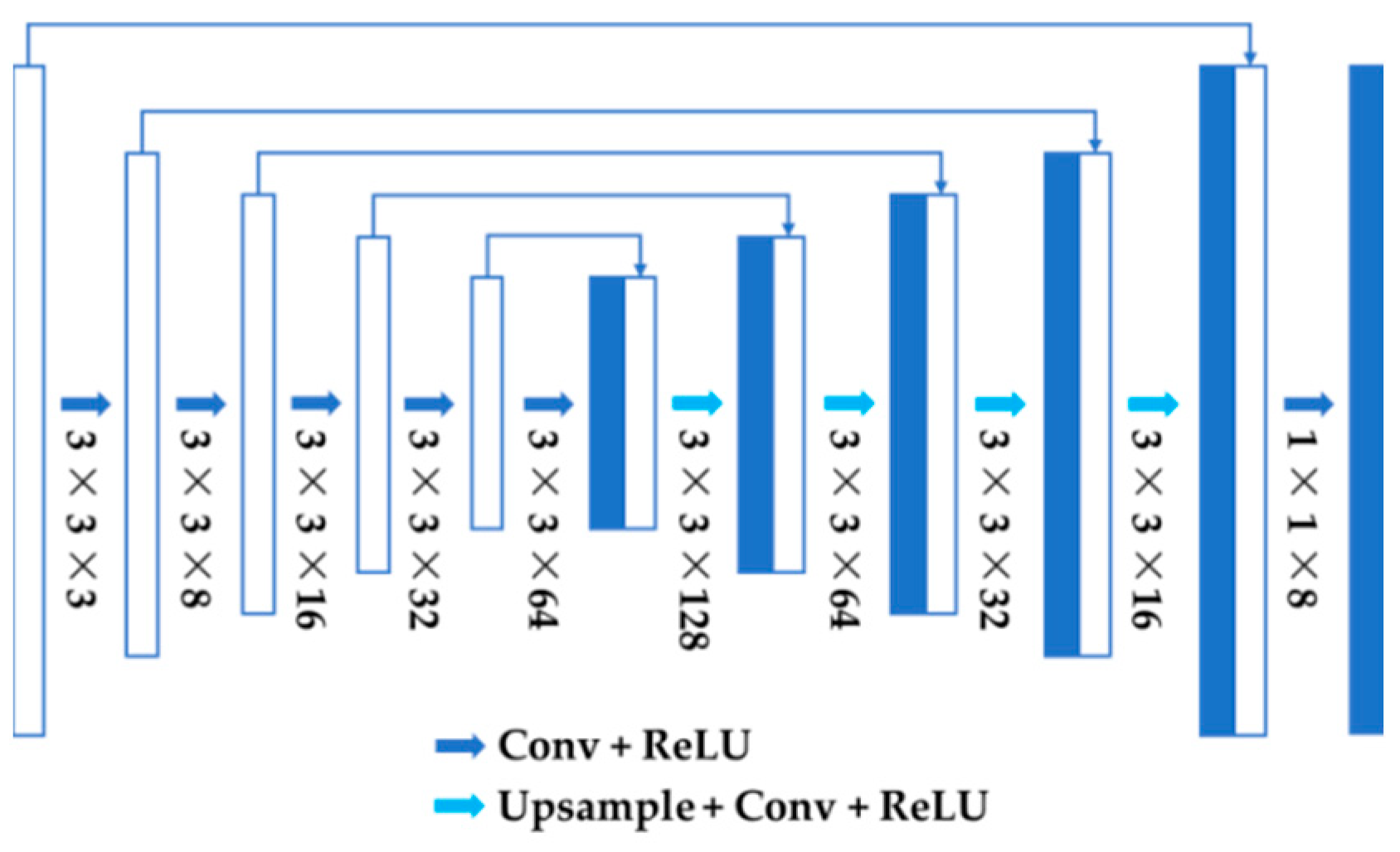
where is -norm. It should be noted that can be any encoder-decoder. Here, U-Net [29] was chosen for precise localization as it consists of a contracting path to capture context and a symmetric expanding path combining high-resolution features with upsampled outputs. The architecture of U-Net is depicted in Figure 4. Inspired by Zheng et al. [30], we superimpose a dynamic graph regularization on the backbone to exploit inherent nonlinear structures of different cells, so that it can be better generalized and adapted to new data. Patches of distance maps are used in an input batch to construct the graphs. Denote an arbitrary distance map patch, which can be a real map or a predicted one , by , where and is the batch size. Regard each as a node and link it only with its 8-nearest neighbors determined by ED [31] in the current batch. The weight of edge between and is computed by
where represents -norm and with . In this way, a localized graph is obtained to exploit local spatial distributions of cells. Moreover, the graph for each input batch is dynamic and evolves with the incoming data as its nodes include predicted distance maps. The graph regularization is defined as
Thus, the loss of the localization network during the pretraining stage is
where is a trade-off coefficient.
After pretraining, online nuclear localization is activated as newly sampled microscopy images are fed to the network . The graph-embedded regressor is fine-tuned in a semi-supervised fashion with both historically labelled data and unlabelled new samples. Let denote the iteration number of online learning, initialized as 0 at the end of pretraining when , the label set and is predicted by the pretrained for image patch . Modify Equation (5) and obtain the graph-regularized regression loss for online localization
where is a trade-off coefficient, and are the distance maps of predicted in the th and the th iterations, respectively, and and indicate the numbers of labelled and unlabelled samples, respectively. It should be noted that both and are dynamic. The former depends on how the label set is expended for online training while the latter is the quantity of new samples fed to the network.
The label set expansion mechanism is designed to leverage the feature adaptation ability of online learning and exploit the information in the unlabelled images. The techniques are as follows. In the th semi-supervised iteration, obtain the binary masks of each unlabelled patch and its predicted distance map by applying the same thresholding and dilation operations, where . The masks reflect major morphology patterns such as nuclear contours and areas. Measure the ED between the binary masks of and and use the reciprocal of ED as the confidence for the predicted map . The lower the distance is, the more reliably the features of the cell image are learned and maintained in the distance map , and the more likely the prediction is correct. Therefore, select predicted maps with the top confidence measurements, rearrange their indexes and add them to the current labelled set for the next iteration. Hence, and is dynamically increased by , whereas .
While the first term in Equation (6) leverages the most confident predictions, the second term pays extra attention to unlabelled samples, even though their predictions may not be so reliable. That unreliability does not mean they are not valuable. Through the iterations, the network gains ability in feature representation. If the network makes similar predictions for unlabelled images in successive iterations, it is probably going into a steady status and approaching its optimum. It is especially desirable to automatically quantify and minimize prediction errors for the unlabelled new data in the online learning scenario. Therefore, the difference between the distance map predicted in the current iteration and that predicted in the last iteration is included in the overall loss. The third term in Equation (6) is the graph regularizer, which depicts the underlying structures of the dynamic labelled and unlabelled datasets that change in each iteration. It can be seen that the semi-supervised regression network can learn from the unlabelled new data while predicting the distance maps. This allows for adaptation to open data and online localization of different nuclei. The Adam optimizer [32] is adopted to perform gradient descent and update the parameters in the backbone.
3.2.3. Postprocessing
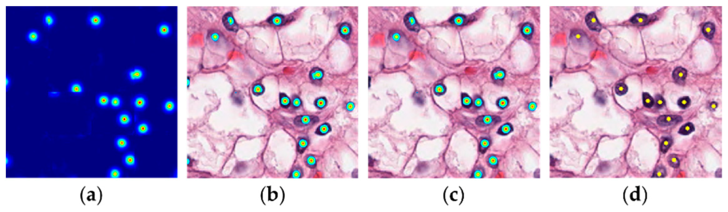
To obtain precise nuclear locations from the predicted distance maps, postprocessing is adopted. This includes three major steps: thresholding, connected region filtering and centroid calculation. Empirically speaking, pixels with small values in a distance map are not usually the centroids of nuclei. Thus, thresholding is used to remove these pixels, as shown in by Figure 5a,b. Given a predicted map , the threshold is set by and the distance map obtained after thresholding.
Because in a microscopy image a nucleus usually consists of a cluster of pixels, its existence is unlikely to be indicated by high-valued but under-sized regions in the distance maps. To avoid false detections, we apply the connected region filtering [33] to remove small regions in and obtain . Figure 5c shows that highlighted regions of very small sizes close to the border of the image are eliminated. Finally, we calculate the coordinate of the centroid of each connected region kept in by averaging the coordinates of pixels in the corresponding region. Regarding the centroids as nuclear positions , we can finally locate the cells of interest in image patch . The yellow dots Figure 5d indicate the estimated nuclear locations.
The implementation details of nuclear localization are summarized in Algorithm 1. It should be noted that numbers of labelled images and unlabelled images before splitting into patches are and , respectively.
| Algorithm 1 Implementation details of the nuclear localizer |
| Input: labelled dataset with dot annotations and newly-sampled unlabelled images ; |
| Step 1 Preprocessing (1a) Split the input images into patches and ; (1b) Convert to distance maps by Equation (1); Step 2 Localization //Pretraining (2a) Pretrain on using Equation (5); (2b) Let the semi-supervised iteration number and ; (2c) Initialize the labelled set as ; //Semi-supervised Online Learning (2d) Feed to and infer ; (2e) Select most confident from ; (2f) Expand the label set as and ; let , and ; (2g) Fine-tune by Equation (6); (2h) Repeat Steps 2d–2g and produce ; Step 3 Postprocessing for (3a) Apply thresholding to and obtain ; (3b) Apply connected region filtering to and obtain ; (3c) Calculate the centroid of each region in and obtain ; end for |
| Output: predicted nuclear locations for . |
3.3. Cell Classification
As shown in Figure 2, after nuclear localization, cell instances are acquired and classifier is employed to identify their cell types. The cell instances are small patches centred at nuclear locations in a microscopy image , where and is the total number of cell instances in . For unlabelled images, the nuclear locations are predicted using Algorithm 1. The instance size is determined empirically. Several cell examples are extracted from the labelled set, the average area for each cell type is calculated, and their values are utilised to determine the instance size. The cell instances thus generated are sufficient for online cell detection. This acquisition technique is very efficient, without engaging complicated implementations or extra training. It enables efficient cell classification for unlabelled images in open datasets, using only approximate knowledge about cell areas instead of precise annotations such as masks or contours of each cell.
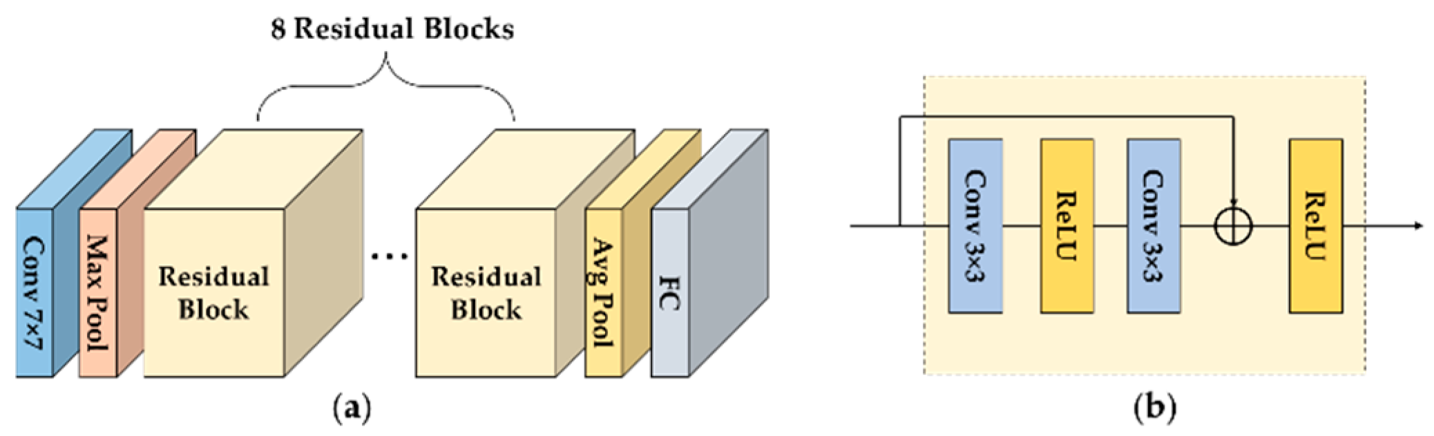
Let the classifier be denoted by , where represents learnable parameters. The inputs are the cell instances resized to the same size () and the outputs are their classes inferred by . To realize online cell detection, we use pretrained deep networks for , because they can be easily fine-tuned by historically labelled data and used for inference of unlabelled cell instances in newly-sampled images. Specifically, SimCLR [34] was selected to leverage its effectiveness and generalizability for cell images. As shown in Figure 6, SimCLR [34] has the same basic architecture as ResNet18 [35], where the residual block adds shortcut connection to avoid degradation of feature representation ability. One difference between ResNet18 and SimCLR is that the former is pretrained with ImageNet [36] and the latter with 57 pathology images [34]. ImageNet contains 1.43 million images with 1000 types, which gives ResNet18 the ability to recognize diversified object patterns. The pathology images enable SimCLR to recognize specific patterns of cells. Another important difference is that SimCLR involves contrastive learning whereas the vanilla ResNet18 does not. SimCLR learns representations by maximizing agreement between differently augmented views of the same sample via contrastive loss. Given strong data augmentation, large batch sizes and long training episodes, contrastive learning is more effective than supervised learning for feature representation [37]. SimCLR benefits from the pathology images and contrastive learning, and is expected to outperform ResNet18 in cell classification for dynamically sampled new data.
The classifier is fine-tuned by Adam [32] on labelled cell instances, , where is number of instances with class labels . To save time, the localization network can be pretrained according to Step 2a in Algorithm 1, and the classifier simultaneously fine-tuned with the historically labelled dataset. After locating cell instances in an unlabelled image, they are fed into the fine-tuned classifier and their cell type is predicted. This way, efficient online cell detection can be performed, with minimal costs incurred for annotations and computations. The process is described in Algorithm 2.
| Algorithm 2 Online cell detection by GeoNet and TPS estimation with PD-L1 IHC slides |
| Input: with dot annotations and newly-sampled unlabelled PD-L1 slides ; |
| Step 1 Initialization (1a) Preprocess and produce as in Step1, Algorithm 1; (1b) Pretrain on using Equation (5); (1c) Fine-tune on as in Section 3.3; Step 2 Online Cell Detection //Localization (2a) Let the semi-supervised iteration number ; for (2b) Feed to and get via Steps 2d–2g in Algorithm 1; (2c) Predict cell locations via Steps 3a–3c in Algorithm 1; //Classification (2d) Obtain from as described in Section 3.3; (2e) Feed to and infer cell classes ; //TPS Estimation (2f) Compute TPS for by Equation (8); end for. |
| Output: predicted nuclear locations , inferred cell classes , and estimated TPS for , where . |
3.4. Application: TPS Estimation
The results of online cell detection obtained via GeoNet can be utilized in many downstream tasks, e.g., quantitative assessment of PD-L1 expression. This is a vital part of PD-L1 immunohistochemical (IHC) assays that have been co-developed as companion or complementary diagnostics for different anti-PD-1/PD-L1 inhibitor drugs [27]. To assess PD-L1 expression, the Dako PD-L1 IHC 22C3 and 28-8 pharmaDx assays employ tumour proportion score (TPS) computed as
where and denote numbers of positive and negative viable tumour cells, respectively. For TPS less than 1%, PD-L1 expression levels are negative. With TPS ranging from 1% to 49%, PD-L1 expression levels are low. When TPS is greater than 49%, PD-L1 expression levels are high. Tumoural expression of PD-L1 is associated with overall survival and adverse events on non-small cell lung cancer (NSCLC) [27]. For patients with untreated metastatic NSCLC with PD-L1 TPS of 50% or greater, it has been reported that first-line pembrolizumab (anti-PD-1/PD-L1 inhibitor) monotherapy improves overall and progression-free survival [38].
In clinical practice, pathologists determine TPS by microscopic examination, which is time-consuming and subjective. It is impractical to detect and count millions of cells contained in large PD-L1 IHC slides. With the proposed GeoNet, we can input new unlabelled PD-L1 slides, then allow the computer to detect tumour cells and estimate TPS automatically. As well as saving manual efforts in annotation and assessment, this method also increases precision in IHC assays. The major procedures are summarized in Algorithm 2. To demonstrate its effectiveness, we applied the method to a set of PD-L1 slides for lung squamous cell carcinoma (LUSC), which is a common type of NSCLC.
4. Results
4.1. Datasets
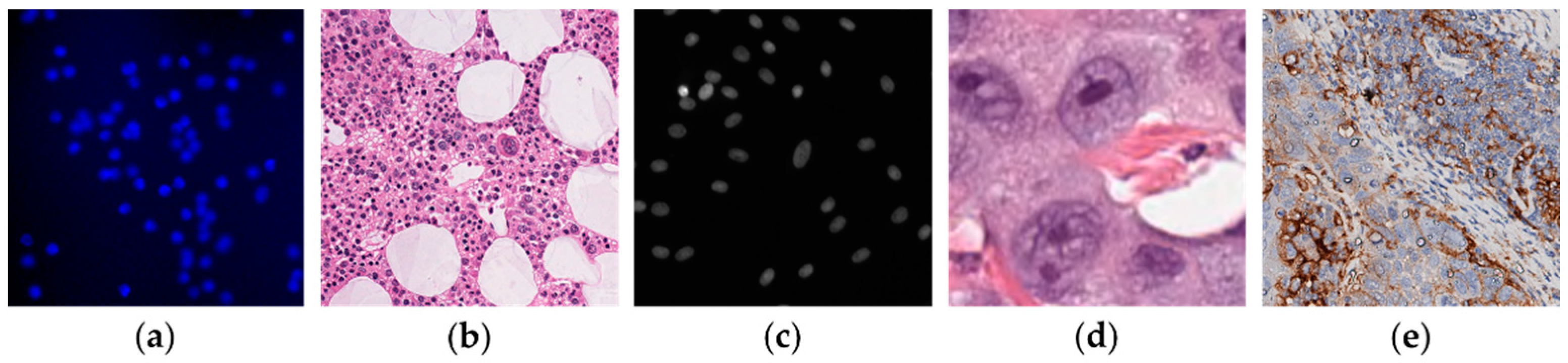
For evaluation of the proposed GeoNet, we used five datasets as illustrated by Figure 7. The first three datasets were used only for online nuclear localization since they were not provided with classification labels. The fourth and fifth were used for the whole pipeline, i.e., nuclear localization plus cell classification. The first two datasets provide a dot annotation on each cell. The last three datasets contain cell-wise segmentation masks. In our experiments, these masks were turned to dot annotations by locating the centre of each mask to generate distance maps. Each dataset was split into subsets of labelled data and unlabelled data. Moreover, the cell detection results on the fifth data set were applied to the downstream task, TPS estimation.
- This dataset comprises bacterial cells in fluorescent-light microscopy images (BCFM) [39]. It contains 200 synthetic images, each with 256 × 256 pixels and 171 ± 64 cells. We randomly selected 32 images from the first 50 images as the labelled set and 50–100 images as unlabelled set (i.e., newly sampled data for online learning).
- The bone marrow (BM) [40] dataset consists of 11 H&E images with 1200 × 1200 pixels, cropped from WSIs (40× magnification) from 8 different patients. We split them into 44 patches, each with 600 × 600 pixels. The labelled set used 15 patches the unlabelled set used 18.
- The Kaggle 2018 Data Science Bowl dataset (Kaggle) [41] contains 670 H&E stained images of different sizes. From these, 335 images were used as the labelled set and 135 as the unlabelled set.
- Pan-Cancer Histology Data for Nuclei Instance Segmentation and Classification (PanNuke) [42] contains 7901 images with 256 × 256 pixels of 19 different tissues, including neoplastic cells, inflammatory cells, connective tissue cells, dead cells and epithelial cells. The data set was supplied split into three subsets. We used the first subset as the labelled set and the second as the unlabelled set.
- LUSC is an in-house dataset, provided by a teaching hospital and a professional pathology diagnosis center [9]. It contains 43 immuostained PD-L1 images with 1000 × 1000 pixels cropped from 4 WSIs scanned with KF-PRO-120 (0.2481 μm/pixel, 40× magnification). We randomly selected 34 images as the labelled set and 9 images as the unlabelled set.
4.2. Implementation Details
For batch-wise input to GeoNet, each image in BCFM, Kaggle and PanNuke was split into smaller patches of 64 × 64 pixels; each 600 × 600 patch in BM was further split into 100 × 100 patches; and each image in LUSC was split into 100 × 100 patches. The batch size was 16. The learning rate for the GeoNet localizer was initialized as 0.0001 and decayed with a factor 0.9 every 20 epochs. For Equation (6), is 0.2 and is 0.2. The number of epochs in the first semi-supervised iteration was 100, and 20 for the rest. The number of selected samples in each iterationwas 1 for BM and LUSC, 2 for BCFM and Kaggle, and 25 for PanNuke. For the classifier, the learning rate was set as 0.00625. Number of epochs was 15. Learning rate was reduced with a factor 0.9 at the 4th, 6th and 8th epoch. Data augmentations including random brightness, contrast, horizontal and vertical flipping were adopted.
To demonstrate the usefulness of the online pipeline, we compared GeoNet with its pretrained model, Graph-Embedded Network (GeNet) [30]. To validate the flexibility of GeoNet, we embedded U-Net [29] and Structured Regression (SR) [1] within the online localizer. The online versions of U-Net and SR are referred to as “O-U-Net” and “O-SR”, respectively. Using the vanilla localizer in GeoNet, we compared SimCLR [34] with ResNet18 [35] as the cell classifier. These two versions are denoted by GeoNet-SimCLR and GeoNet-ResNet18. F1-score, precision, and recall [10] were employed to evaluate cell detection performance. For localization metrics, if the predicted location is within a circle with a radius of 12 from the real location, the predicted location is accurate. All methods were implemented on a workstation equipped with an NVIDIA GeForce RTX 2080 Ti.
4.3. Experimental Analysis
4.3.1. Detection Performance
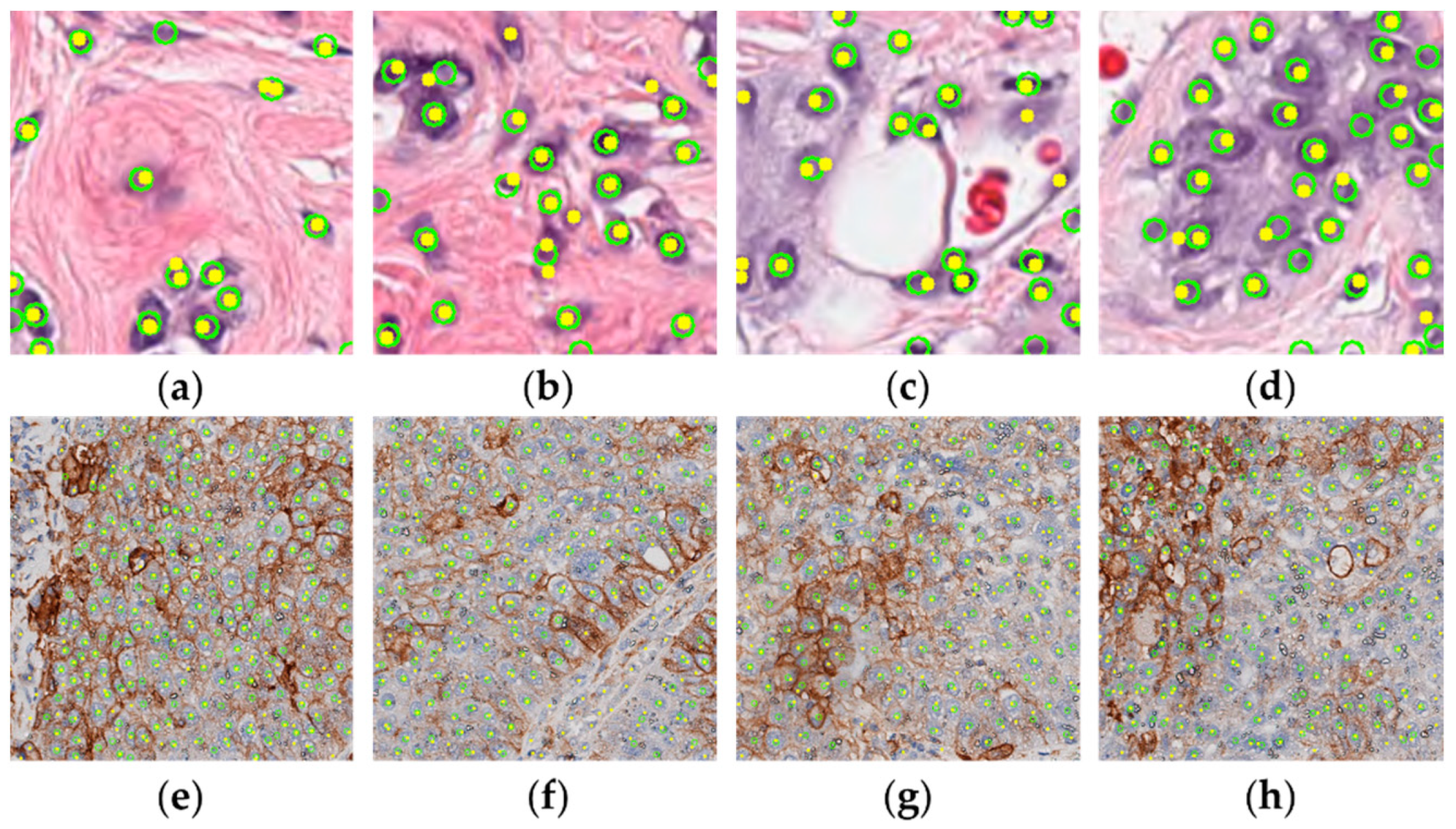
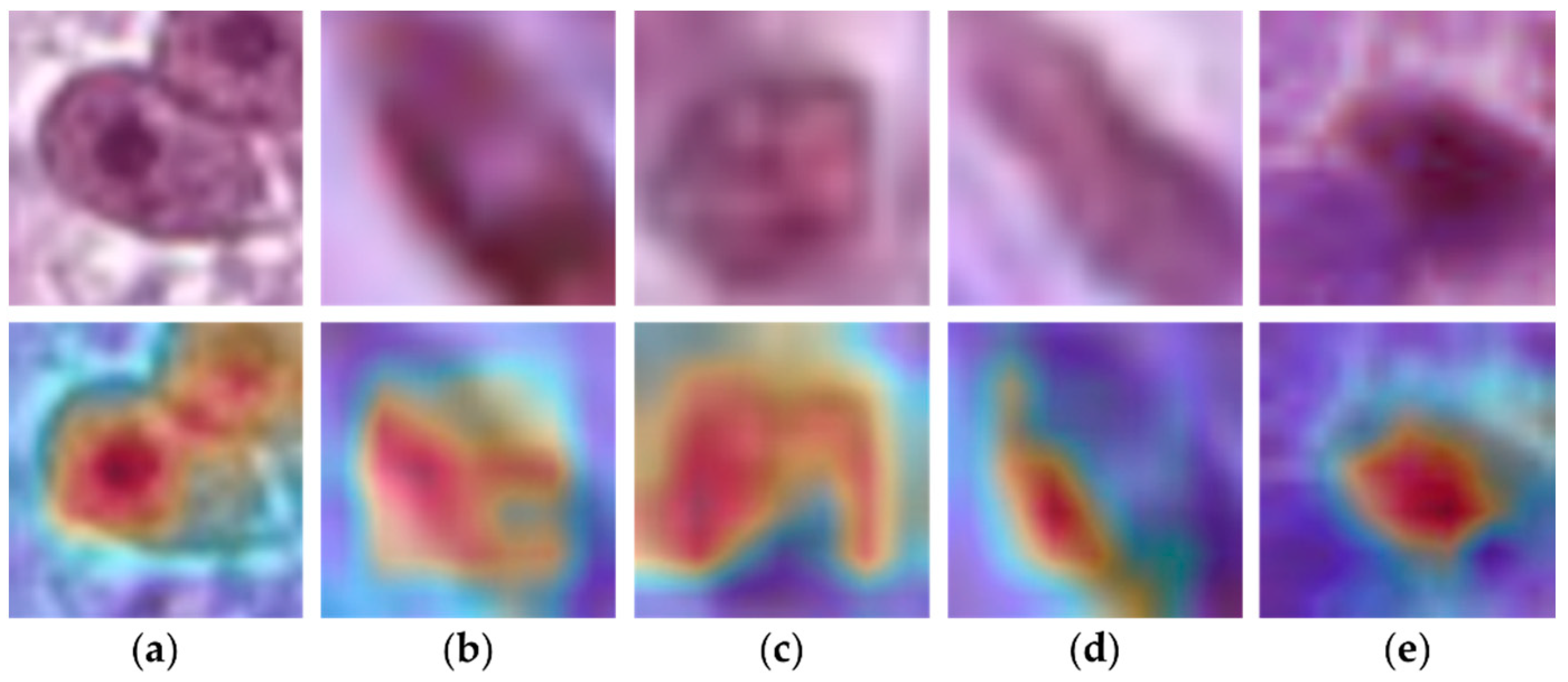
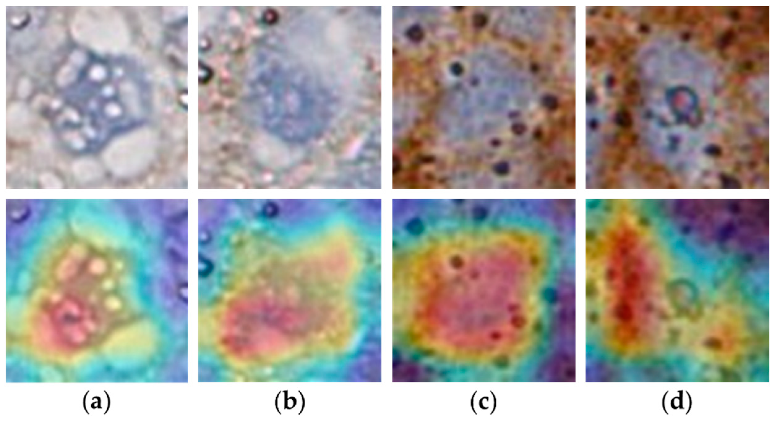
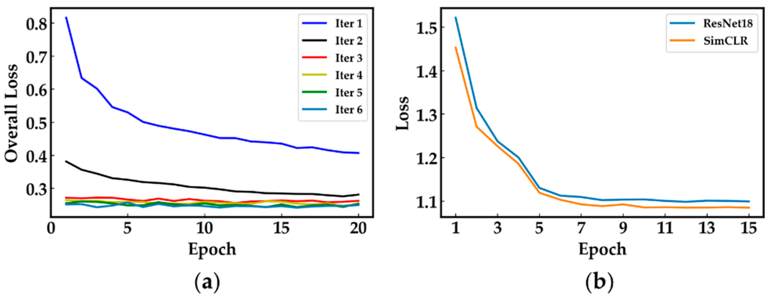
We used the PanNuke and LUSC data sets to validate the efficacy and efficiency of the proposed online learning network, GeoNet. As illustrated in Figure 8, the localizer in GeoNet can automatically locate different cell types in the unlabelled images. Most predicted nuclear locations represented by yellow dots are within the green circles that indicate the real locations. Figure 9 and Figure 10 visualize the saliency maps for cell instances of different classes acquired at the predicted locations, showing that the classifier in GeoNet can represent discriminative patterns. Table 1 and Table 2 give the classification indexes. Since classification is the last step in the online detection pipeline, the classification results are the final detection outcomes. They show that GeoNet can generate cell instances without manual annotations and accurately detect cells in unlabelled images in a semi-supervised fashion. Meanwhile, GeoNet embedded with SimCLR as the classifier (GeoNet-SimCLR) outperforms the ResNet18, since SimCLR is pretrained on pathology images and involves contrastive learning. As indicated by Table 2, GeoNet-SimCLR can accurately identify negative and positive tumour cells in the PD-L1 slides, thus being applicable to TPS estimation for LUSC. Figure 11 demonstrates the efficiency of the online learning process. Figure 11a shows that the loss curve of the localizer converges in each semi-supervised iteration. Figure 11b shows that the loss curve of each classifier converges rapidly. Because both the localizer and classifier function correctly, the whole framework illustrated by Figure 2 is successfully implemented.
However, there is still room for improvement. As can be seen in Section 4.1, PanNuke is a class-unbalanced dataset [42]. Dead cells account for its smallest proportion, 4.7%, and neoplastic cells account for the greatest proportion, 37.7%. As Table 1 shows, whichever one of GeoNet-SimCLR or GeoNet-ResNet18 is applied, the poorest classification indexes are those of dead cells. Meanwhile, the indexes of neoplastic cells are much better. This problem can be addressed by performing class-related data augmentation or introducing class-wise reweighting to the loss of GeoNet.
4.3.2. Detailed Localization Results
We used the BCFM, BM, Kaggle and PanNuKe datasets to test the localization performance of GeoNet. Table 3 shows that GeoNet outperforms the other methods in general. For all datasets, GeoNet yielded higher F1-scores than the competing models, especially the supervised ones, indicating its feature representation ability. The F1-scores of GeoNet are higher than those of O-U-Net, validating the use of the dynamic graph regularizer to enable GeoNet to learn inherent nonlinear structures of cells and gain better generalizability than O-U-Net for newly captured unlabelled images. Furthermore, almost every semi-supervised model outperformed its supervised counterpart on the unlabelled sets. This not only demonstrates that semi-supervised optimization can increase localization precision, but also indicates the flexibility of GeoNet. The proposed method can utilize almost any encoder-decoder to regress nuclear locations. As illustrated by Figure 11a, the loss curve of every iteration converges, indicating that the label set expansion mechanism for the semi-supervision avoided the introduction of errors and can exploit information in the unlabelled images. Thus, it can be seen that GeoNet exhibits good feature adaption ability, which is important for online cell detection in dynamically imported images.
To further demonstrate the efficiency of the proposed online learning pipeline, we recorded the time costs of O-U-Net, O-SR and GeoNet for semi-supervised training and prediction for the BCFM dataset. Table 4 indicates that the time consumptions, especially the online prediction time are acceptable. For example, GeoNet took only 0.35 s to locate all the cells in each unlabelled image (around 171 cells per image). O-SR spent the most time on training due to its complex structure. GeoNet costs more training time than O-U-Net because the construction of the dynamic graph requires extra time. However, the prediction time of O-U-Net and GeoNet were close. According to Table 3, GeoNet located nuclei more accurately than O-U-Net. This means that GeoNet is a practical method for online cell detection in unknown images.
4.3.3. TPS Estimation Errors
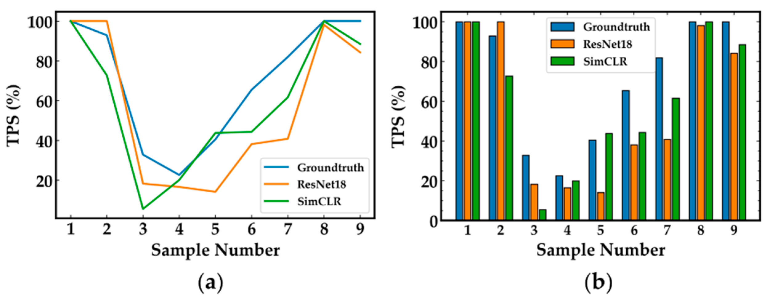
The detection results of GeoNet were satisfactory, and were applied to TPS estimation. As described in Section 3.4, pathologists usually assess PD-L1 expression by TPS for diagnosis and treatment of NSCLC. Table 5 shows the predicted TPS values and relative errors for GeoNet-ResNet18 and GeoNet-SimCLR applied to LUSC. Predicted TPS values of GeoNet-SimCLR and GeoNet-ResNet18 are both greater than 49%, suggesting that PD-L1 expression levels are high. As described in Section 3.4, pathologists make clinical diagnosis according to PD-L1 expression levels rather than a precise TPS value. Therefore, the exact values of predicted TPS will not impact pathologists’ decisions if the TPS values fall into the predefined ranges (<1%, 1–49%, >49%). Figure 12 shows the TPS of every unlabelled image in LUSC and the histogram of the unlabelled set. It can be seen that GeoNet-SimCLR outperformed GeoNet-ResNet18 in most TPS estimation cases. Although there were some errors, especially when real TPS values were lower than 50%, these were not great enough to alter diagnosis because the predicted TPS values were in the same range as the real ones. To improve TPS estimation in GeoNet, we could add a branch after the classifier to regress positive and negative cell counts as well as TPS values.
5. Conclusions
We propose a novel graph-embedded online learning network, namely GeoNet, for cell detection with dot annotations. With its efficient label set expansion mechanism, GeoNet uses historical data and reliable new samples to optimize the model in an online learning fashion. In this way, GeoNet can learn features from unknown data while at the same time efficiently predicting nuclear locations. By involving a dynamic graph regularizer, GeoNet can exploit inherent nonlinear structures of cells to improve generalizability. Thus, GeoNet can adapt to new images with various cell patterns. Moreover, GeoNet is a practical network as its detection results can be applied to downstream tasks such as TPS estimation. Experimental results validate the flexibility and effectiveness of GeoNet.
Author Contributions
Conceptualization, Z.C.; methodology, Z.C.; software, Y.Z. and J.C.; validation, J.C. and Y.Z.; formal analysis, Z.C. and J.C.; investigation, Y.Z.; resources, Z.C.; data curation, Y.Z.; writing—original draft preparation, J.C. and Z.C; writing—review and editing, J.C. and Z.C; visualization, Y.Z.; supervision, Z.C.; project administration, Z.C.; funding acquisition, Z.C. All authors have read and agreed to the published version of the manuscript.
Funding
This work was funded in part by the “Chenguang Program” supported by Shanghai Education Development Foundation and Shanghai Municipal Education Commission under Grant 18CG38, the National Natural Science Foundation of China under Grant 61702094 and the Science and Technology Commission of Shanghai Municipal under Grant 17YF1427400.
Institutional Review Board Statement
Not applicable.
Informed Consent Statement
Not applicable.
Data Availability Statement
Not applicable.
Conflicts of Interest
The authors declare no conflict of interest.
References
- Xie, Y.; Xing, F.; Shi, X.; Kong, X.; Su, H.; Yang, L. Efficient and robust cell detection: A structured regression approach. Med. Image Anal. 2018, 44, 245–254. [Google Scholar] [CrossRef] [PubMed]
- Saranya, A.; Kottilingam, K. A Survey on Bone Fracture Identification Techniques using Quantitative and Learning Based Algorithms. In Proceedings of the 2021 International Conference on Artificial Intelligence and Smart Systems (ICAIS), Coimbatore, India, 25–27 March 2021; pp. 241–248. [Google Scholar]
- Graham, S.; Vu, Q.D.; Raza, S.E.A.; Azam, A.; Tsang, Y.W.; Kwak, J.T.; Rajpoot, N. Hover-Net: Simultaneous segmentation and classification of nuclei in multi-tissue histology images. Med. Image Anal. 2019, 58, 101563. [Google Scholar] [CrossRef] [PubMed] [Green Version]
- Gu, Z.; Cheng, J.; Fu, H.; Zhou, K.; Hao, H.; Zhao, Y.; Zhang, T.; Gao, S.; Liu, J. CE-Net: Context Encoder Network for 2D Medical Image Segmentation. IEEE Trans. Med. Imaging 2019, 38, 2281–2292. [Google Scholar] [CrossRef] [PubMed] [Green Version]
- Song, J.; Xiao, L.; Lian, Z. Contour-Seed Pairs Learning-Based Framework for Simultaneously Detecting and Segmenting Various Overlapping Cells/Nuclei in Microscopy Images. IEEE Trans. Image Process. 2018, 27, 5759–5774. [Google Scholar] [CrossRef]
- Xing, F.; Xie, Y.; Yang, L. An Automatic Learning-Based Framework for Robust Nucleus Segmentation. IEEE Trans. Med. Imaging 2016, 35, 550–566. [Google Scholar] [CrossRef]
- Li, J.; Yang, S.; Huang, X.; Da, Q.; Yang, X.; Hu, Z.; Duan, Q.; Wang, C.; Li, H. Signet Ring Cell Detection With a Semi-supervised Learning Framework. arXiv 2019, arXiv:1907.03954. [Google Scholar]
- Ying, H.; Song, Q.; Chen, J.; Liang, T.; Gu, J.; Zhuang, F.; Chen, D.Z.; Wu, J. A semi-supervised deep convolutional framework for signet ring cell detection. Neurocomputing 2021, 453, 347–356. [Google Scholar] [CrossRef]
- Chen, Z.; Chen, Z.; Liu, J.; Zheng, Q.; Zhu, Y.; Zuo, Y.; Wang, Z.; Guan, X.; Wang, Y.; Li, Y. Weakly Supervised Histopathology Image Segmentation With Sparse Point Annotations. IEEE J. Biomed. Health Inform. 2021, 25, 1673–1685. [Google Scholar] [CrossRef]
- Chen, Y.; Liang, D.; Bai, X.; Xu, Y.; Yang, X. Cell Localization and Counting Using Direction Field Map. IEEE J. Biomed. Health Inform. 2022, 26, 359–368. [Google Scholar] [CrossRef]
- Huang, Z.; Ding, Y.; Song, G.; Wang, L.; Geng, R.; He, H.; Du, S.; Liu, X.; Tian, Y.; Liang, Y.; et al. BCData: A Large-Scale Dataset and Benchmark for Cell Detection and Counting. In Proceedings of the Medical Image Computing and Computer Assisted Intervention—MICCAI 2020, Lima, Peru, 4–8 October 2020; pp. 289–298. [Google Scholar]
- Song, T.H.; Sanchez, V.; Daly, H.E.; Rajpoot, N.M. Simultaneous Cell Detection and Classification in Bone Marrow Histology Images. IEEE J. Biomed. Health Inform. 2019, 23, 1469–1476. [Google Scholar] [CrossRef] [Green Version]
- Xie, Y.; Xing, F.; Kong, X.; Su, H.; Yang, L. Beyond Classification: Structured Regression for Robust Cell Detection Using Convolutional Neural Network. In Proceedings of the Medical Image Computing and Computer-Assisted Intervention—MICCAI 2015, Munich, Germany, 5–9 October 2015; pp. 358–365. [Google Scholar]
- Hagos, Y.B.; Narayanan, P.L.; Akarca, A.U.; Marafioti, T.; Yuan, Y. ConCORDe-Net: Cell Count Regularized Convolutional Neural Network for Cell Detection in Multiplex Immunohistochemistry Images. In Proceedings of the Medical Image Computing and Computer Assisted Intervention—MICCAI 2019, Shenzhen, China, 13–17 October 2019; pp. 667–675. [Google Scholar]
- Saha, M.; Chakraborty, C. Her2Net: A Deep Framework for Semantic Segmentation and Classification of Cell Membranes and Nuclei in Breast Cancer Evaluation. IEEE Trans. Image Process. 2018, 27, 2189–2200. [Google Scholar] [CrossRef] [PubMed]
- Zhang, H.; Grunewald, T.; Akarca, A.U.; Ledermann, J.A.; Marafioti, T.; Yuan, Y. Symmetric Dense Inception Network for Simultaneous Cell Detection and Classification in Multiplex Immunohistochemistry Images. In Proceedings of the MICCAI Workshop on Computational Pathology, Strasbourg, France, 27 September–1 October 2021; pp. 246–257. [Google Scholar]
- Hou, L.; Nguyen, V.; Kanevsky, A.B.; Samaras, D.; Kurc, T.M.; Zhao, T.; Gupta, R.R.; Gao, Y.; Chen, W.; Foran, D.; et al. Sparse autoencoder for unsupervised nucleus detection and representation in histopathology images. Pattern Recogn. 2019, 86, 188–200. [Google Scholar] [CrossRef] [PubMed]
- Javed, S.; Mahmood, A.; Dias, J.; Werghi, N.; Rajpoot, N. Spatially Constrained Context-Aware Hierarchical Deep Correlation Filters for Nucleus Detection in Histology Images. Med. Image Anal. 2021, 72, 102104. [Google Scholar] [CrossRef] [PubMed]
- Xue, Y.; Bigras, G.; Hugh, J.; Ray, N. Training Convolutional Neural Networks and Compressed Sensing End-to-End for Microscopy Cell Detection. IEEE Trans. Med. Imaging 2019, 38, 2632–2641. [Google Scholar] [CrossRef] [Green Version]
- Theera-Umpon, N. White Blood Cell Segmentation and Classification in Microscopic Bone Marrow Images. In Proceedings of the Fuzzy Systems and Knowledge Discovery, Changsha, China, 27–29 August 2005; Springer: Berlin/Heidelberg, Germany, 2005; pp. 787–796. [Google Scholar]
- Sharma, H.; Zerbe, N.; Heim, D.; Wienert, S.; Behrens, H.-M.; Hellwich, O.; Hufnagl, P. A Multi-resolution Approach for Combining Visual Information using Nuclei Segmentation and Classification in Histopathological Images. In Proceedings of the 10th International Conference on Computer Vision Theory and Applications, Berlin, Germany, 11–14 March 2015; pp. 37–46. [Google Scholar]
- Yang, X.; Li, H.; Zhou, X. Nuclei Segmentation Using Marker-Controlled Watershed, Tracking Using Mean-Shift, and Kalman Filter in Time-Lapse Microscopy. IEEE Trans. Circuits Syst. Regul. Pap. 2006, 53, 2405–2414. [Google Scholar] [CrossRef]
- Veta, M.; van Diest, P.J.; Kornegoor, R.; Huisman, A.; Viergever, M.A.; Pluim, J.P.W. Automatic Nuclei Segmentation in H&E Stained Breast Cancer Histopathology Images. PLoS ONE 2013, 8, e70221. [Google Scholar]
- Achanta, R.; Shaji, A.; Smith, K.; Lucchi, A.; Fua, P.; Süsstrunk, S. SLIC Superpixels Compared to State-of-the-Art Superpixel Methods. IEEE Trans. Pattern Anal. Mach. Intell. 2012, 34, 2274–2282. [Google Scholar] [CrossRef] [Green Version]
- Mualla, F.; Schöll, S.; Sommerfeldt, B.; Maier, A.K.; Steidl, S.; Buchholz, R.; Hornegger, J. Unsupervised Unstained Cell Detection by SIFT Keypoint Clustering and Self-labeling Algorithm. In Proceedings of the Medical Image Computing and Computer-Assisted Intervention—MICCAI 2014, Boston, MA, USA, 20 June–29 August 2014; pp. 377–384. [Google Scholar]
- Tofighi, M.; Guo, T.; Vanamala, J.K.P.; Monga, V. Prior Information Guided Regularized Deep Learning for Cell Nucleus Detection. IEEE Trans. Med. Imaging 2019, 38, 2047–2058. [Google Scholar] [CrossRef] [Green Version]
- Liu, J.; Zheng, Q.; Mu, X.; Zuo, Y.; Xu, B.; Jin, Y.; Wang, Y.; Tian, H.; Yang, Y.; Xue, Q.; et al. Automated tumor proportion score analysis for PD-L1 (22C3) expression in lung squamous cell carcinoma. Sci. Rep. 2021, 11, 15907. [Google Scholar] [CrossRef]
- Hondelink, L.M.; Hüyük, M.; Postmus, P.E.; Smit, V.; Blom, S.; von der Thüsen, J.H.; Cohen, D. Development and validation of a supervised deep learning algorithm for automated whole-slide programmed death-ligand 1 tumour proportion score assessment in non-small cell lung cancer. Histopathology 2022, 80, 635–647. [Google Scholar] [CrossRef]
- Ronneberger, O.; Fischer, P.; Brox, T. U-Net: Convolutional Networks for Biomedical Image Segmentation. In Proceedings of the Medical Image Computing and Computer-Assisted Intervention—MICCAI 2015, Munich, Germany, 5–9 October 2015; pp. 234–241. [Google Scholar]
- Zheng, Y.; Chen, Z.; Zuo, Y.; Guan, X.; Wang, Z.; Mu, X. Manifold-Regularized Regression Network: A Novel End-to-End Method for Cell Counting and Localization. In Proceedings of the 4th International Conference on Innovation in Artificial Intelligence, Xiamen, China, 8–11 May 2020; pp. 121–124. [Google Scholar]
- Dong, W.; Moses, C.; Li, K. Efficient k-nearest neighbor graph construction for generic similarity measures. In Proceedings of the 20th international conference on World wide web, Hyderabad, India, 28 March–1 April 2011; pp. 577–586. [Google Scholar]
- Kingma, D.P.; Ba, J. Adam: A Method for Stochastic Optimization. arXiv 2014, arXiv:1412.6980. [Google Scholar]
- Remove Small Objects Function. Available online: https://scikit-image.org/docs/stable/api/skimage.morphology.html#skimage.morphology.remove_small_objects (accessed on 11 March 2022).
- Ciga, O.; Xu, T.; Martel, A.L. Self supervised contrastive learning for digital histopathology. arXiv 2020, arXiv:2011.13971. [Google Scholar] [CrossRef]
- He, K.; Zhang, X.; Ren, S.; Sun, J. Deep Residual Learning for Image Recognition. In Proceedings of the 2016 IEEE Conference on Computer Vision and Pattern Recognition (CVPR), Las Vegas, NV, USA, 27–30 June 2016; pp. 770–778. [Google Scholar]
- Deng, J.; Dong, W.; Socher, R.; Li, L.J.; Kai, L.; Li, F.-F. ImageNet: A large-scale hierarchical image database. In Proceedings of the 2009 IEEE Conference on Computer Vision and Pattern Recognition (CVPR), Miami Beach, FL, USA, 20–25 June 2009; pp. 248–255. [Google Scholar]
- Chen, T.; Kornblith, S.; Norouzi, M.; Hinton, G. A Simple Framework for Contrastive Learning of Visual Representations. arXiv 2020, arXiv:2002.05709. [Google Scholar]
- Mok, T.S.K.; Wu, Y.L.; Kudaba, I.; Kowalski, D.M.; Cho, B.C.; Turna, H.Z.; Castro, G., Jr.; Srimuninnimit, V.; Laktionov, K.K.; Bondarenko, I.; et al. Pembrolizumab versus chemotherapy for previously untreated, PD-L1-expressing, locally advanced or metastatic non-small-cell lung cancer (KEYNOTE-042): A randomised, open-label, controlled, phase 3 trial. Lancet 2019, 393, 1819–1830. [Google Scholar] [CrossRef]
- Lempitsky, V.; Zisserman, A. Learning To count objects in images. In Proceedings of the 23rd International Conference on Neural Information Processing Systems, Vancouver, BC, Canada, 6–9 December 2010; pp. 1324–1332. [Google Scholar]
- Kainz, P.; Urschler, M.; Schulter, S.; Wohlhart, P.; Lepetit, V. You Should Use Regression to Detect Cells. In Proceedings of the Medical Image Computing and Computer-Assisted Intervention—MICCAI 2015, Munich, Germany, 5–9 October 2015; pp. 276–283. [Google Scholar]
- Kaggle 2018 Data Science Bowl. Available online: https://www.kaggle.com/c/data-science-bowl-2018/data (accessed on 11 March 2022).
- Gamper, J.; Alemi Koohbanani, N.; Benet, K.; Khuram, A.; Rajpoot, N. PanNuke: An Open Pan-Cancer Histology Dataset for Nuclei Instance Segmentation and Classification. In Proceedings of the Digital Pathology, Athens, Greece, 29 August–1 September 2019; pp. 11–19. [Google Scholar]
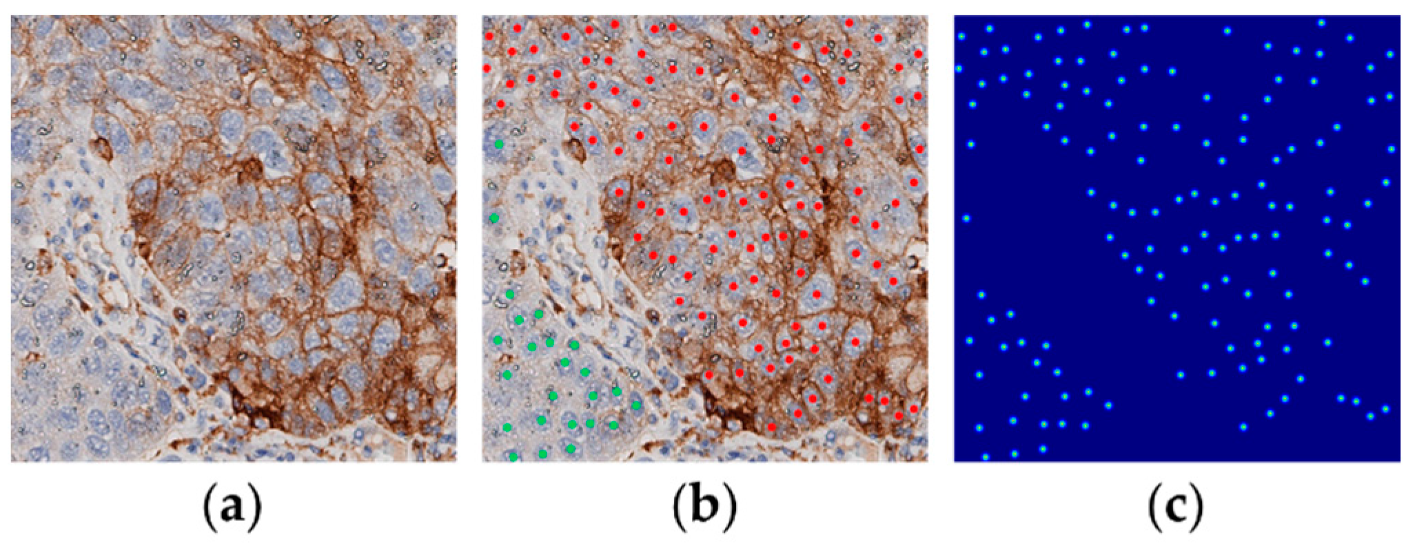
Figure 1.
(a) An example of PD-L1 slides from the LUSC data set, (b) dot annotations (red indicates positive viable tumour cells and green negative ones) and (c) distance map generated from the dot annotations.
Figure 1.
(a) An example of PD-L1 slides from the LUSC data set, (b) dot annotations (red indicates positive viable tumour cells and green negative ones) and (c) distance map generated from the dot annotations.

Figure 2.
GeoNet pipeline.

Figure 3.
GeoNet nuclear localizer.

Figure 4.
Architecture of the backbone for nuclear localization.

Figure 5.
Visualization of postprocessing. (a) A predicted distance map. (b) The original image overlaid with the distance map after thresholding. (c) The original image overlaid with the distance map after connected region filtering. (d) The original image overlaid with centroids (yellow dots) in connected regions, regarded as the estimated nuclear locations.

Figure 6.
(a) Architecture of ResNet18 [35]/SimCLR [34] used for cell classification with (b) details of the residual block.

Figure 7.
Five sets of cell images, (a) BCFM, (b) BM (c) Kaggle, (d) PanNuke, and (e) LUSC.

Figure 8.
Visualized detection results of GeoNet on PanNuke and LUSC. (a–d) and (e–h) show nuclear localization in PanNuke and LUSC, respectively. Yellow dots stand for predicted locations and green circles for real locations.
Figure 8.
Visualized detection results of GeoNet on PanNuke and LUSC. (a–d) and (e–h) show nuclear localization in PanNuke and LUSC, respectively. Yellow dots stand for predicted locations and green circles for real locations.

Figure 9.
Different types of cell instances in PanNuke (the first row) with their classification saliency maps (the second row). (a) neoplastic cell, (b) epithelial cell, (c) inflammatory cell, (d) connective cell and (e) dead cell.
Figure 9.
Different types of cell instances in PanNuke (the first row) with their classification saliency maps (the second row). (a) neoplastic cell, (b) epithelial cell, (c) inflammatory cell, (d) connective cell and (e) dead cell.

Figure 10.
Different types of cell instances in LUSC (the first row) with their classification saliency maps (the second row). (a,b) are negative cells and (c,d) are positive cells.
Figure 10.
Different types of cell instances in LUSC (the first row) with their classification saliency maps (the second row). (a,b) are negative cells and (c,d) are positive cells.

Figure 11.
(a) Localization loss curves and (b) classification loss curves of GeoNet for PanNuke.

Figure 12.
(a) TPS value of each image in the unlabelled LUSC set. (b) Histogram of (a).


Table 1.
Numerical detection results for unlabelled images in the PanNuke data set.
| Cell Type | GeoNet-ResNet18 | GeoNet-SimCLR | ||||
|---|---|---|---|---|---|---|
| Precision | Recall | F1-Score | Precision | Recall | F1-Score | |
| Neoplastic | 0.626 | 0.792 | 0.700 | 0.621 | 0.806 | 0.702 |
| Epithelial | 0.497 | 0.414 | 0.452 | 0.535 | 0.343 | 0.418 |
| Inflammatory | 0.627 | 0.668 | 0.647 | 0.636 | 0.667 | 0.651 |
| Connective | 0.575 | 0.539 | 0.556 | 0.588 | 0.517 | 0.550 |
| Dead | 0.551 | 0.326 | 0.410 | 0.535 | 0.343 | 0.418 |
Table 2.
Numerical detection results for unlabelled images in the LUSC data set.
| Cell Type | GeoNet-ResNet18 | GeoNet-SimCLR | ||||
|---|---|---|---|---|---|---|
| Precision | Recall | F1-Score | Precision | Recall | F1-Score | |
| Negative | 0.671 | 0.772 | 0.718 | 0.692 | 0.781 | 0.734 |
| Positive | 0.800 | 0.703 | 0.748 | 0.812 | 0.731 | 0.769 |
Table 3.
Evaluation of cell localization for the unlabelled images of each data set.
| Model | BCFM | BM | Kaggle | PanNuke | ||||||||
|---|---|---|---|---|---|---|---|---|---|---|---|---|
| Precision | Recall | F1-Score | Precision | Recall | F1-Score | Precision | Recall | F1-Score | Precision | Recall | F1-Score | |
| U-Net | 0.920 | 0.916 | 0.918 | 0.742 | 0.810 | 0.775 | 0.767 | 0.841 | 0.802 | 0.652 | 0.691 | 0.671 |
| SR | 0.758 | 0.816 | 0.786 | 0.855 | 0.932 | 0.892 | 0.720 | 0.745 | 0.732 | 0.648 | 0.667 | 0.657 |
| GeNet | 0.935 | 0.914 | 0.924 | 0.844 | 0.961 | 0.899 | 0.847 | 0.829 | 0.838 | 0.687 | 0.702 | 0.694 |
| O-U-Net | 0.924 | 0.920 | 0.922 | 0.765 | 0.813 | 0.789 | 0.768 | 0.868 | 0.815 | 0.690 | 0.711 | 0.700 |
| O-SR | 0.764 | 0.824 | 0.793 | 0.875 | 0.933 | 0.903 | 0.755 | 0.785 | 0.770 | 0.677 | 0.680 | 0.678 |
| GeoNet | 0.935 | 0.919 | 0.927 | 0.868 | 0.950 | 0.907 | 0.850 | 0.846 | 0.848 | 0.712 | 0.730 | 0.721 |
Table 4.
Time costs of semi-supervised training and prediction for BCFM.
| Model | Time Cost for Training (s/image) | Time Cost for Prediction (s/image) |
|---|---|---|
| O-U-Net | 410.57 | 0.34 |
| O-SR | 820.98 | 0.54 |
| GeoNet | 658.14 | 0.35 |
Table 5.
Average TPS values of the unlabelled set of LUSC.
| Estimation Method | GeoNet-ResNet18 | GeoNet-SimCLR |
|---|---|---|
| Real TPS | 70.7% | |
| Predicted TPS | 56.7% | 59.6% |
| Relative Error | 13.9% | 11.1% |
Publisher’s Note: MDPI stays neutral with regard to jurisdictional claims in published maps and institutional affiliations. |
© 2022 by the authors. Licensee MDPI, Basel, Switzerland. This article is an open access article distributed under the terms and conditions of the Creative Commons Attribution (CC BY) license (https://creativecommons.org/licenses/by/4.0/).
Share and Cite
MDPI and ACS Style
Chen, J.; Zhu, Y.; Chen, Z. Graph-Embedded Online Learning for Cell Detection and Tumour Proportion Score Estimation. Electronics 2022, 11, 1642. https://0-doi-org.brum.beds.ac.uk/10.3390/electronics11101642
AMA Style
Chen J, Zhu Y, Chen Z. Graph-Embedded Online Learning for Cell Detection and Tumour Proportion Score Estimation. Electronics. 2022; 11(10):1642. https://0-doi-org.brum.beds.ac.uk/10.3390/electronics11101642
Chicago/Turabian StyleChen, Jinhao, Yuang Zhu, and Zhao Chen. 2022. "Graph-Embedded Online Learning for Cell Detection and Tumour Proportion Score Estimation" Electronics 11, no. 10: 1642. https://0-doi-org.brum.beds.ac.uk/10.3390/electronics11101642
Note that from the first issue of 2016, this journal uses article numbers instead of page numbers. See further details here.