Automatic Weight Prediction System for Korean Cattle Using Bayesian Ridge Algorithm on RGB-D Image

Abstract

Weighting the Hanwoo (Korean cattle) is very important for Korean beef producers when selling the Hanwoo at the right time. Recently, research is being conducted on the automatic prediction of the weight of Hanwoo only through images with the achievement of research using deep learning and image recognition. In this paper, we propose a method for the automatic weight prediction of Hanwoo using the Bayesian ridge algorithm on RGB-D images. The proposed system consists of three parts: segmentation, extraction of features, and estimation of the weight of Korean cattle from a given RGB-D image. The first step is to segment the Hanwoo area from a given RGB-D image using depth information and color information, respectively, and then combine them to perform optimal segmentation. Additionally, we correct the posture using ellipse fitting on segmented body image. The second step is to extract features for weight prediction from the segmented Hanwoo image. We extracted three features: size, shape, and gradients. The third step is to find the optimal machine learning model by comparing eight types of well-known machine learning models. In this step, we compared each model with the aim of finding an efficient model that is lightweight and can be used in an embedded system in the real field. To evaluate the performance of the proposed weight prediction system, we collected 353 RGB-D images from livestock farms in Wonju, Gangwon-do in Korea. In the experimental results, random forest showed the best performance, and the Bayesian ridge model is the second best in MSE or the coefficient of determination. However, we suggest that the Bayesian ridge model is the most optimal model in the aspect of time complexity and space complexity. Finally, it is expected that the proposed system will be casually used to determine the shipping time of Hanwoo in wild farms for a portable commercial device.

1. Introduction

Livestock raising is the world’s most expensive industry for grazing and the production of feed grains. In addition, the global demand for livestock products is expected to further increase due to population growth, rising incomes and urbanization. An increase in market demand for meat and milk products, to provide food for a growing population, has led to a rapid growth in the scale of cattle and pig enterprises globally. As the scale of animal husbandry around the world increases, addressing the issue of animal management becomes more essential. Due to the current scale of production, there is increasing awareness that the monitoring of animals can no longer be performed by farmers in the traditional way and requires the adoption of new digital technologies. Therefore, it is possible to improve the job satisfaction of livestock farmers by detecting the health status or abnormal behavior of livestock at an early stage in real time, reducing the livestock production cost and managing economic loss due to disease and death. For this reason, livestock producers are demanding the development of a new technology that can monitor livestock in real time, the application of new sensors, and the development of a new system that can shorten the integrated processing time in order to produce high-quality livestock products.

On the one hand, the body weight (BW) of livestock during livestock production is a very important and widely used feature that has a significant impact on feed consumption, breeding potential, social behavior, energy balance, and overall farm management. It may be used indirectly in the assessment of health and welfare status for livestock, and in the determination of time to market for animals. Additionally, large or abrupt changes in BW might indicate the presence of a disease, improper housing conditions, welfare problems, feeding errors or inefficient genetic selection. Therefore, continued monitoring and maintaining a livestock weight history can help ensure timely interventions in the livestock diet and health and increase the efficiency of genetic selection. Furthermore, a great advantage of tracking weight gain is that it enables one to identify the best time to market animals because animals that have already reached the point of slaughter represent a burden for feedlot. However, taking livestock such as cattle and pigs out of the kennel and guiding them on the scales is a laborious and stressful activity for both livestock and breeders. In addition, this process may give a lot of stress to the livestock, which may reduce the weight of the livestock [1]. With these problems in mind, some research teams and companies are developing solutions that automatically track the weight of livestock in the kennel using image processing techniques based on computer vision technology.

Therefore, studies to solve these problems until now can be largely divided into two fields. One is using image processing technology and computer vision technology [2,3,4,5,6,7,8], and the other is a method using various deep learning technologies such as CNN or R-CNN. First, the approach method using image processing technology and the computer vision approach proceeds through the following steps. In the first step, images are collected by capturing the appearance of livestock with a 2D or 3D camera, and in the second step livestock are sorted manually or automatically based on the acquired image method to extract the appropriate features. The third step is to predict the weight of livestock using a traditional regression model. Since this approach does not require a large amount of learning data, it is a method that can be usefully used when it is difficult to actually acquire a large amount of data in the field. However, these computer vision and image processing approaches require some manual work in steps such as image and feature selection, image segmentation, and shape measurement value extraction. Therefore, in high-throughput applications that can handle the weight of large numbers of livestock, this approach prevents the integration of multiple stages of processing. So, it difficult to develop commercial solutions for full automation. Second, the method using various deep learning algorithms is an approach to automate most tasks of estimating the weight of livestock with methods recently proposed by various scholars [9]. This approach automatically extracts a feature vector from an input image using an artificial neural network structure such as CNN, and uses the extracted feature vector as an input to a deep learning network to automatically predict the weight of livestock. However, in this deep-learning-based approach, the number of parameters constituting the model is too large, and a large number of learning data are required to train them. Therefore, it is considered that it is practically impossible to obtain a large amount of data for learning such a deep learning model in the field. For this reason, it is thought that a model based on computer vision technology that requires a little manual work is more useful than a method based on deep learning that has an advantage in automation for the model available in the actual livestock field.

Therefore, in this paper, we are going to propose a prediction system that can automatically predict the weight of Korean cattle using computer vision techniques and various machine learning models. First, in Section 2, we will briefly review various domestic and foreign prior studies related to the problem of predicting the weight of various livestock, such as cattle and pigs and sheep. Next, Section 3 briefly describes the collection of Korean cattle image data, which is the topic of interest in this thesis, and also presents the overall structure of a system that can predict the weight of Korean cattle. Here, we describe in detail the segmentation method, feature extraction method, and various machine learning methods used to predict the weight of Korean cattle, which are three components of the proposed prediction system. Additionally, Section 4 discusses an experiment conducted to confirm the performance of the proposed system using the collected Korean cattle image data. Finally, in Section 5, the results obtained in this study and future research directions are presented as a conclusion.

2. Related Works

Here, we will briefly review the previous studies published on the problem of predicting the weight of livestock. First, we would like to introduce a few review papers that comprehensively introduce research on the problem of predicting the weight of livestock. Femandes et al. [10] presented significant developments that have been made in computer vision system (CVS) applications in animal and veterinary sciences and highlighted areas in which further research is still needed before the full deployment of CVS in breeding programs and commercial farms. Nasirahmadi et al. [11] described the state of art in 3D imaging systems along with 2D cameras for effectively identifying livestock behaviors and presented automated approaches for the monitoring and investigation of cattle and pig feeding, drinking, lying, locomotion, aggressive and reproductive behaviors. The performance of developed systems is reviewed in terms of sensitivity, specificity, accuracy, error rate and precision. These technologies can support the farmer by monitoring normal behaviors and early detection of abnormal behaviors in large-scale enterprises. Wang et al. [12] published a comprehensive review paper on machine learning methods for predicting the weight of livestock from digital images. In their paper, they classified the methods that can predict the weight of livestock into four major fields, which are traditional approaches, computer vision approaches, computer vision and ML approaches, and computer vision and deep learning approaches, respectively. In addition, they described in general what techniques were used and what differences were in the areas of feature extraction, feature selection, regression and the learning model, which are parts of the prediction system [6,7,8].

Next, livestock raised in barns can be broadly classified into subdivisions, which are cattle, pigs, sheep, and chickens, respectively. Here, we are going to review previous studies on methods of predicting the weight of cattle in breeding. Seo and his colleagues [13] have developed a technique that can use image processing technology to automatically measure cow body parameters, reducing labor and breeding time. The image processing system designed and built for this project consisted of a PC, grabber card and two cameras located on the side and top of the model cow. Based on the study results, we compared the parameters of chest depth, armor height, pelvic arch height, trunk length, slope trunk length, chest width, hip width, churl width, and pin bone width of real cows. The cow model values and actual measured data were obtained, and most errors were less than 5%, showing relatively good results. Tasdemir and Ozkin [14] developed a model that can predict the weight of a Holstein cow using an artificial neural network that determines the body size by a photogrammetry method. For the body characteristics they considered the cow’s Wither height, hip height, body length, and hip width. In addition, they estimated the cow’s weight using the body characteristics obtained from the image, and then calculated the correlation coefficient between the estimated weight and the actual observed weight. Statistical analysis shows that artificial neural networks can be safely used for live weight prediction. Hung et al. [15] proposed a novel approach to measuring the body dimensions of live Qinchuan cattle with transfer learning. They pre-trained the convolutional layer constituting the proposed Kd-network with the shapeNet dataset, which is widely used in deep learning. Moreover, a fully connected layer that predicts body measurements was used as TrAdaBoost. Additionally, to evaluate the performance of the proposed system, they predicted the body size of a cow using point cloud data and confirmed that it showed an accuracy of 93.6%. Rudenko et al. [16] considered the problem of weight estimation of cows using a convolutional neural-network-based method for animal recognition and proposed breed identification in combination with an epipolar geometric approach for measuring the size of an individual. In addition, they additionally used the information on animal size and breed for LW estimation by a multilayer perceptron-based predictive model. Additionally, it was confirmed that the proposed approach can be used to replace the traditional direct observation and measurement. The proposed system can be widely used in the management of modern farms. Pradana et al. [17] segmented the cow body from the cow’s lateral image using a localized region-based active contour model. Additionally, the number of pixels constituting the divided body is extracted as a feature vector. Next, they proposed a system for predicting the weight of a cow using the extracted feature vector as an input to the linear regression model. Weber et al. [18] analyzed both the body measurements of the Girolando cattle and measurements extracted from the images to create a model to understand which measurements further explained the cow’s weight. Therefore, they physically measured 34 Girolando cattle (two males and 32 females), for the following traits: heart girth (HGP), circumference of the abdomen, body length, occipito-ischial length, wither height, and hip height. In addition, from images of the dorsum and the body lateral area of these animals, they allowed measurements of hip width (HWI), body length, tail distance to the neck, dorsum area (DAI), dorsum perimeter, wither height, hip height, body lateral area, perimeter of the lateral area, and rib height. Finally, they developed a linear regression model that can predict the weight of a cow using various measured body characteristics. Gjergji et al. [19] explored different deep learning model performances in the regression task of predicting cattle weight. They analyzed convolutional neural networks, RNN/CNN networks, Recurrent Attention Models, and Recurrent Attention Models with Convolutional Neural Networks. They also showed the performance and speed comparisons of these networks for the problem of cattle weight prediction, and they found that convolutional neural networks are most performant. Alvarez et al. [20] used transfer learning and ensemble modeling techniques to significantly extend the performance of automated systems based on CNNs to further improve the body condition score (BCS) estimation accuracy. They also showed that the improved system has achieved good estimation results in comparison with the base system. Additionally, several papers related to the problem of measuring the weight of Korean cattle were published. Lee et al. [21] developed a model for estimating the carcass weight of Hanwoo cattle as a function of body measurements using three different modeling approaches: multiple regression analysis, partial least square regression analysis, and a neural network. They measured a total of 20 variables related to carcass weight and body measurements to estimate the cold carcass weight of Korean cattle using three predictive methods. Jang et al. [22] estimated the body weight of Korean cattle (Hanwoo) using a three-dimensional image. They acquired a top view image of Korean cattle using a ToF camera and a stereo vision camera, and used a multiple linear regression model to estimate the body weight. From the experimental results, they confirmed that the coefficient of determination for both the TOF image and the stereo vision image was improved when the age variable correlated with the weight was incorporated. Additionally, it was confirmed that the weight estimation error was significantly reduced under the condition of excluding calves under 6 months of age.

3. Materials and Methods

3.1. Korean Cattle Image Collection

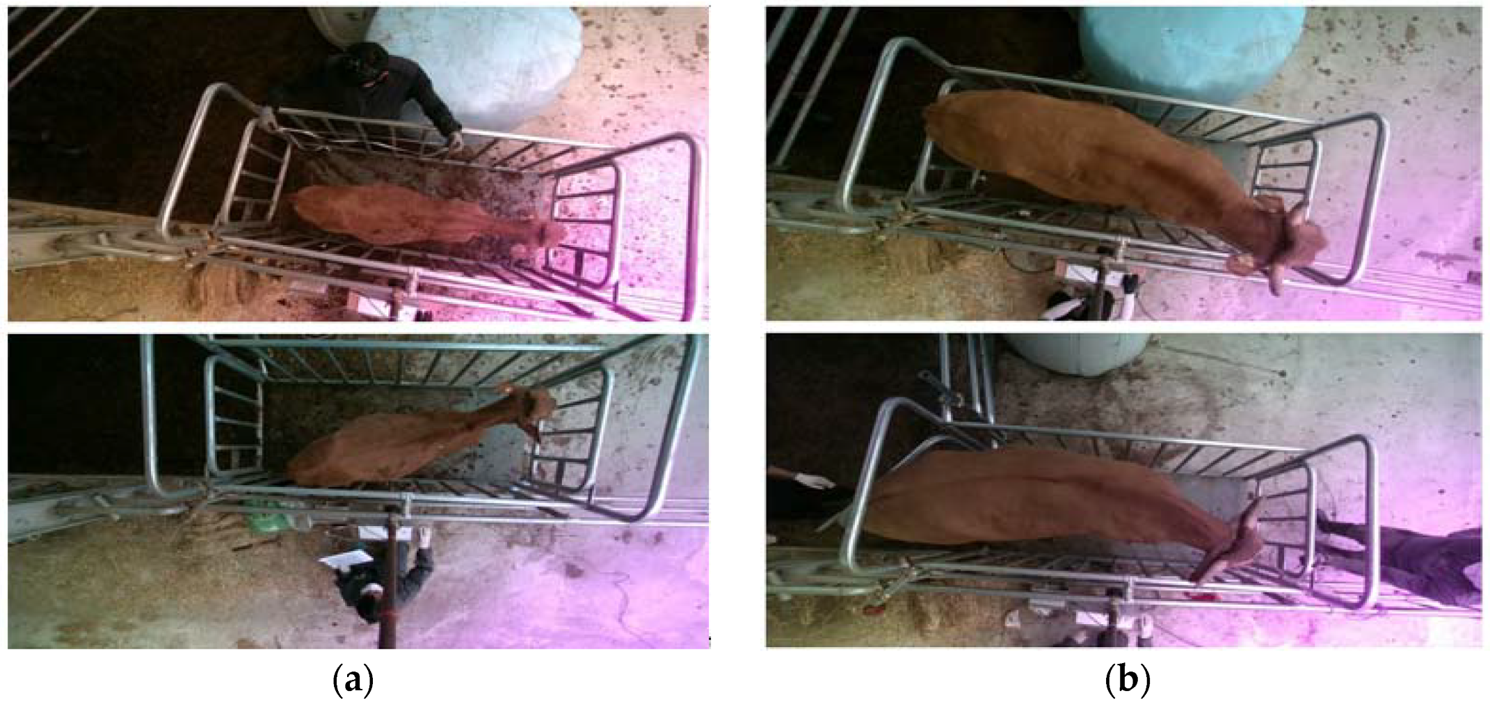
We constructed data by measuring 3D images and weights of 15 Korean cattle, including 8 bulls and 7 cows at 26 weeks of age, at 2-week intervals from 22 June 2021 to 17 August 2021 as shown in Figure 1. The collected image dataset consisted of 353 data sets by manually selecting 3~5 frames from the depth and color images captured using Intel RealSense depth cameras D455. The following figure shows a sample of RGB-D images of male and female Korean cattle collected from a livestock farm.

3.2. Proposed Method

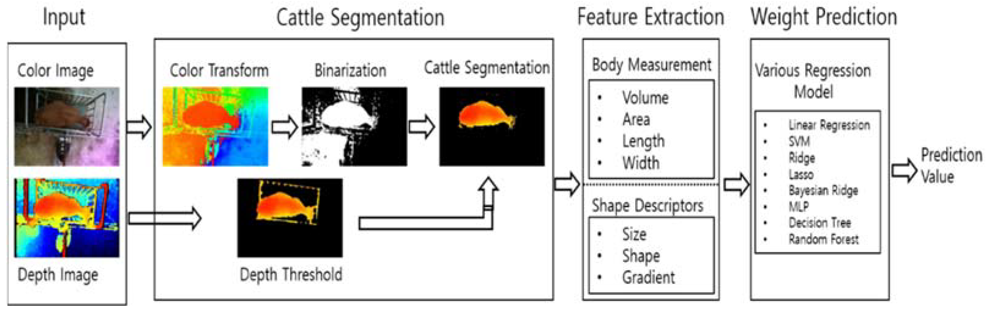
In order to predict the weight of Korean cattle from the input video image, several steps are required to fill the gap between raw data and cattle weight. In the first step, it is necessary to segment cattle from each image in the collected video data. This is to accurately separate the cattle from the background in the image. The second step is to extract the features most appropriate for predicting their weight from the segmented cattle images. The third step is to predict the weight of a calf using appropriate regression models based on the extracted feature vectors. The architecture of our prediction system of cattle weight is illustrated in Figure 2.

3.2.1. Cattle Segmentation

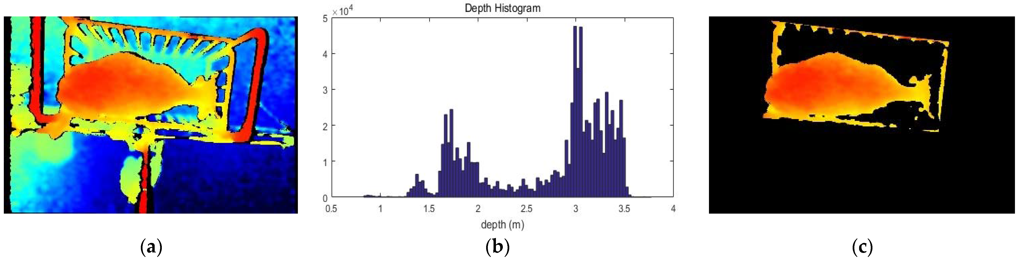
In this section, we have implemented object segmentation algorithms that can segment cattle in RGB-D images. This method, based on the threshold of histogram, is a method of applying, respectively, two thresholds of histogram for each of the HSI image and the depth image in the RGB-D image and then combining them to obtain final segmentation [13]. First, we consider a depth image containing cattle. In this image, the cattle are close to the camera and the background is given away from the camera. Therefore, all areas except cattle are considered as background. At this time, in order to extract cattle area, (a) histogram is created from the given depth image as shown in (b) of Figure 3.

Next, from the histogram of the given depth information, two threshold values are selected: the lower limit and the upper limit. As shown in the following Equation (1), if the depth of each pixel in the image falls within the selected upper and lower limits, a value of 255 is assigned; otherwise, 0 is assigned.

$$\mathrm{f}\left(\mathrm{x},\mathrm{y}\right)=\left\{\begin{array}{c}255{ \mathrm{if} \mathrm{T}}_{\mathrm{a}}\le \mathrm{d}\left(\mathrm{x},\mathrm{y}\right) \le { \mathrm{T}}_{\mathrm{b}} \\ 0 \mathrm{otherwise} \end{array}\right.$$

(1)

Here, the selection of the two-lower bound (${\mathrm{T}}_{\mathrm{a}}$) and upper bound (${\mathrm{T}}_{\mathrm{b}}$) is made in two steps. The threshold value of the first step is set arbitrarily considering the height of the camera and the height of Korean cattle. First-order binarization is performed using the threshold set in the first step, and the median value of the depth of the binarized region is calculated. In the second step, 0.35 is subtracted and added from the previously obtained median value and then two computed values are determined as the lower and upper limits of the final threshold. Figure 3 shows the image segmentation process using thresholds based on depth images.

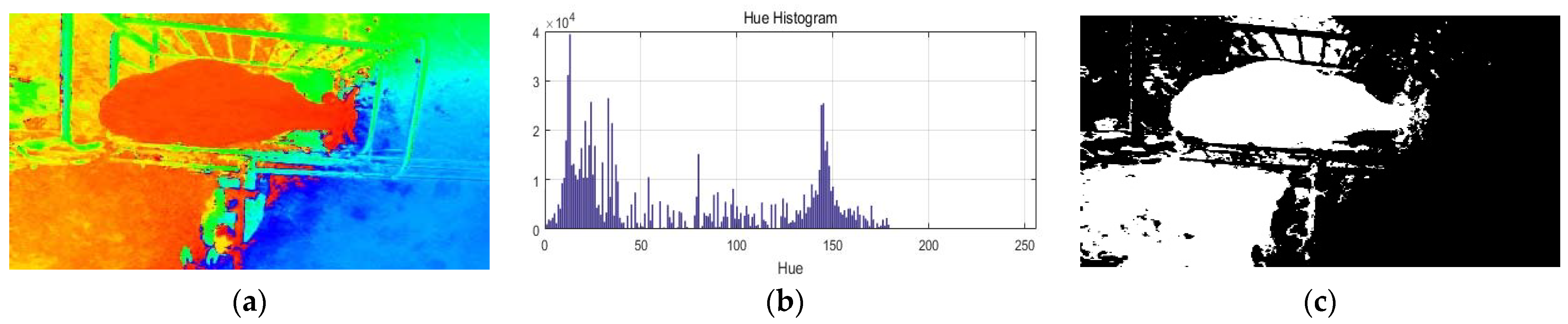
Second, we consider RGB color images to segment cattle. Here, we convert the RGB image to the HSV image and create a histogram for the Hue component. At this time, appropriate color ranges ${\mathrm{T}}_{\mathrm{a}}$ and ${\mathrm{T}}_{\mathrm{b}}$ are selected, and if the Hue component value is within the selected color range, 255 is assigned; otherwise, a value of 0 is assigned.

$$\mathrm{f}\left(\mathrm{x},\mathrm{y}\right)=\left\{\begin{array}{c}255{ \mathrm{if} \mathrm{T}}_{\mathrm{a}}\le \mathrm{H}\left(\mathrm{x},\mathrm{y}\right)\le { \mathrm{T}}_{\mathrm{b}} \\ 0 \mathrm{otherwise} \end{array}\right.$$

(2)

Here, the threshold is a process of two steps. In the first step, we manually segment several images into Korean cattle and the background to find a statistical range for the skin color of Korean cattle. In the second step, we perform HSV color conversion on the segmented cattle region and generate a histogram for the Hue component. Additionally, then we select the minimum and maximum values of the histogram as the lower and upper limits of the threshold. Figure 4 shows the process of segmenting Korean cattle based on color components for color images.

Third, the final segmentation image is constructed by combining the two segmentation results using the following procedure.

• Case 1: If the two segmentation results match and they are assigned to the background, then the corresponding pixel is assigned to the background.
• Case 2: If the two segmentation results match and they are assigned to the foreground, then the corresponding pixel is assigned to the foreground.
• Case 3: If the two segmentation results do not match, the pixel is assigned as an object or background according to the segmentation result given by using the depth image.

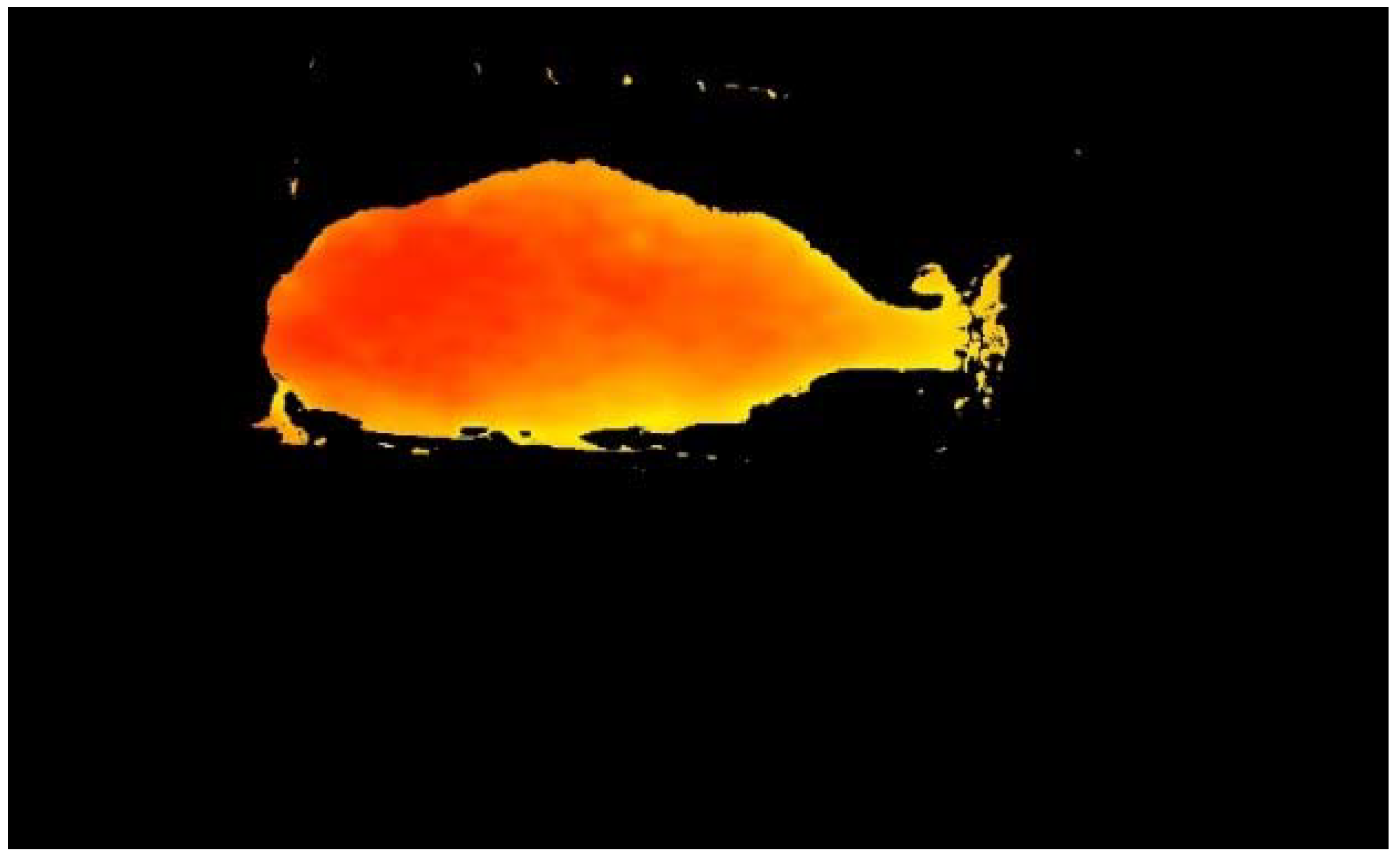
Figure 5 shows the final segmentation result obtained by combining the two segmentation results for RGB-D images.

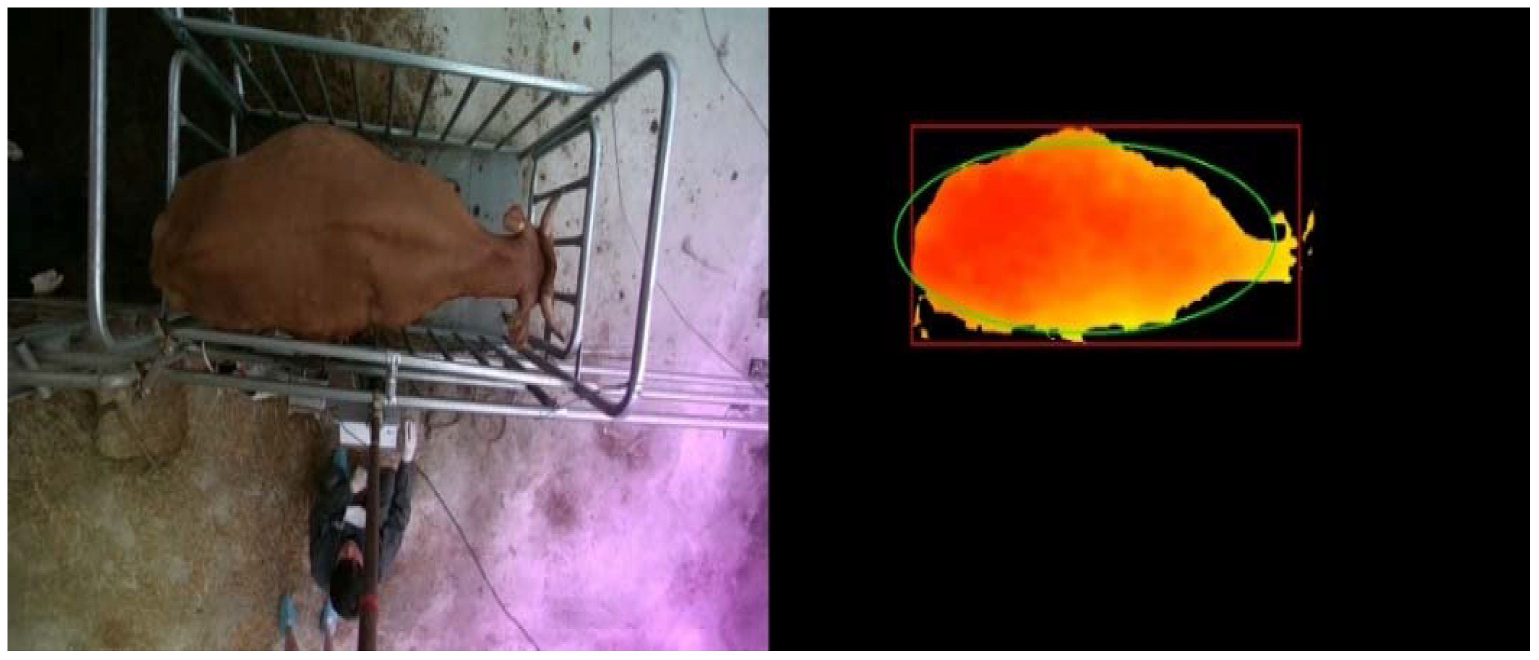
Finally, we create a bounding box for the segmented RGB-D cattle image by the following procedure. (1) Apply morphological filtering to fill convex hulls or small holes in the combined segment results. (2) Search for contour including cattle in the segmented image. (3) Find the upper, lower, left, and right outermost points from the completed contour. (4) Make a bounding box connecting the outermost points. Figure 6 shows the bounding box image finally created from the cattle image.

3.2.2. Position Correction

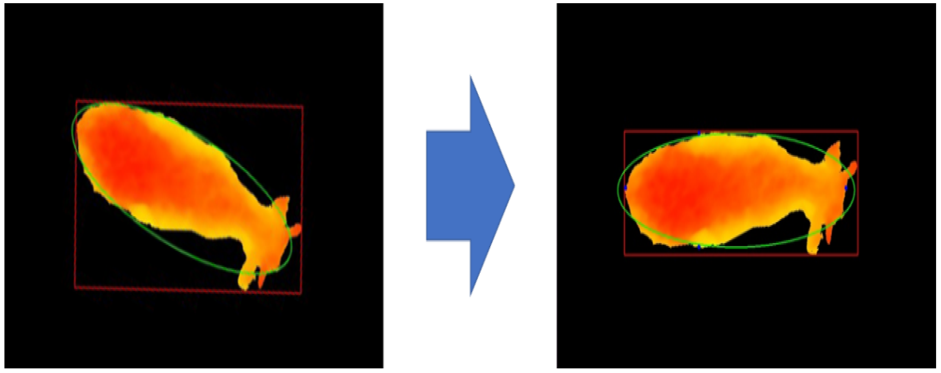
In order to obtain accurate body measurements of Korean cattle from segmented images, the posture of Korean cattle is most important. In other words, in order to predict the exact weight from body measurements such as size and shape, Korean cattle must maintain a straight line from the head to the tail. However, in reality, it is very difficult to maintain a constant posture without movement for the time required to measure the body measurements. Therefore, we need to correct the posture according to the movement of Korean cattle. To create a constant pose in the camera top-view image, we fit an ellipse to the segmented binary image by using Hough transform. Additionally, the posture of Korean cattle was corrected by rotating the image according to the position of the fitted ellipse. We use the Hough transform to estimate the ellipse that can best fit the outline of the previously segmented Korean cattle region. The fitted ellipse has a center for the segmented region, a major axis according to the length of the Korean cattle, a minor axis perpendicular to this length, and an angle of rotation of the ellipse. Figure 7 shows how the long axis, minor axis, and angle of the ellipse were obtained by fitting an ellipse to the segmented Korean cattle image, and the posture was adjusted by rotating the Korean cattle image by the obtained angle of the ellipse.

3.2.3. Feature Extraction

Here, we will consider the extraction method of various feature vectors required to predict the weight of a segmented 3D cattle image. The group of these extracted feature vectors is largely classified into two areas, which are body measurements and size and shape kernel descriptors [22,23,24].

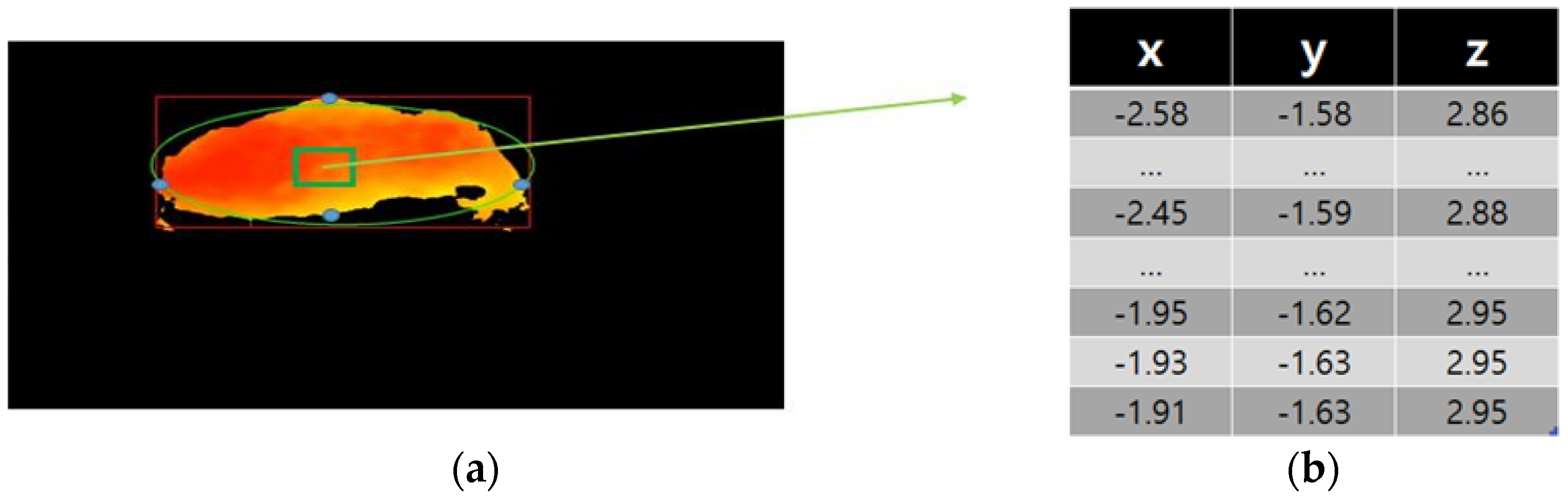
First, we will consider the characteristics that can measure the cattle body. The body measurements for real cattle are length, widths, area, and volume at equidistant locations across the back of the cattle, from the shoulders to the rump. Here, in order to calculate the four body measurements, point cloud coordinates are obtained from the segmented cattle image. The point cloud is obtained by mapping from image coordinates to real-world coordinates using the SDK provided by the depth camera manufacturer. Figure 8 shows the segmented 3D cattle image and the point cloud coordinates for the pixels in some selected box.

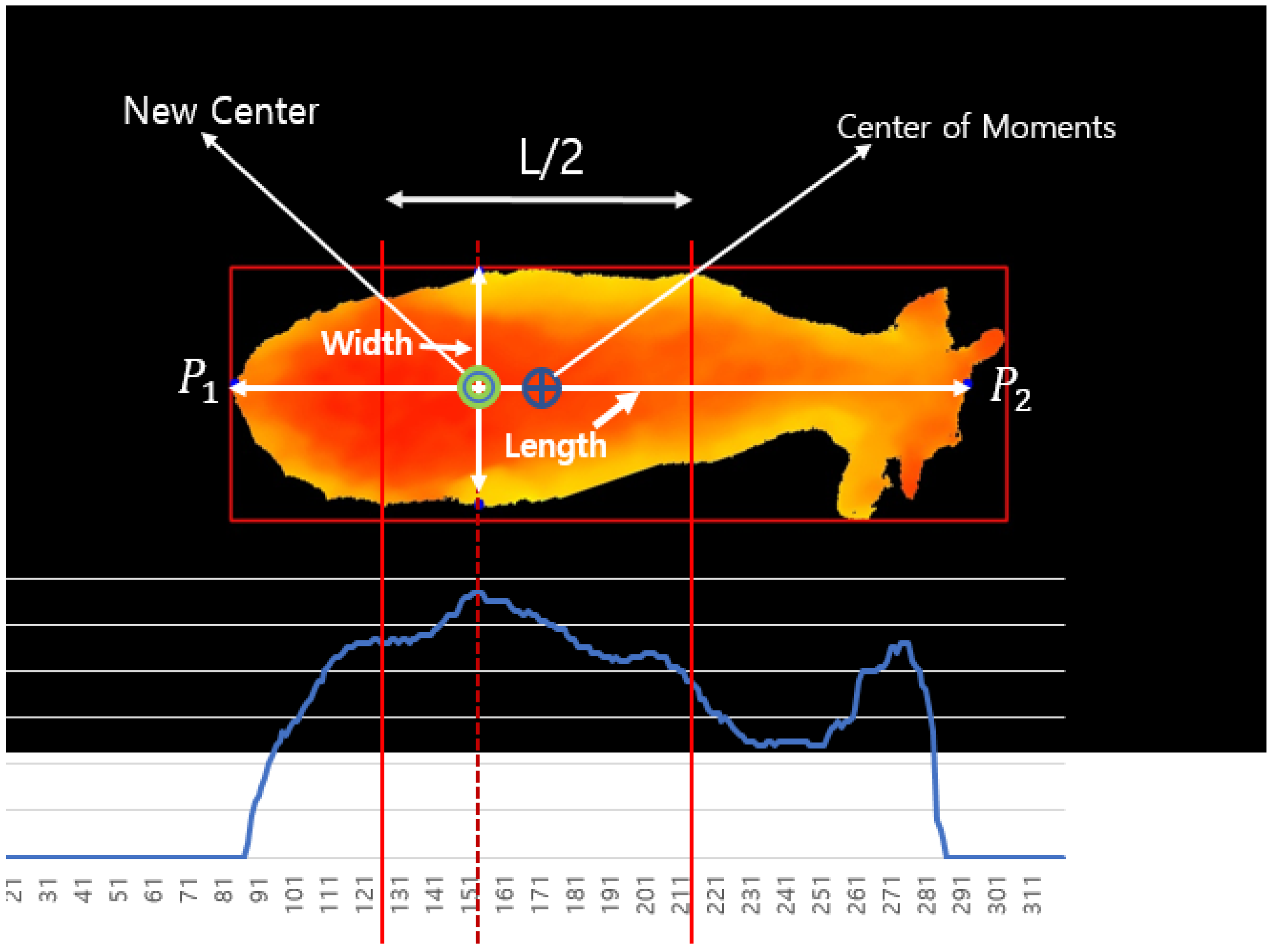
To calculate the length, the centroid coordinates are calculated using the moment from the segmented binary Korean cattle image as shown in Figure 9. We pick both horizontal endpoints P1 and P2 of the binary image from the center. Using the point cloud coordinates of the selected two points P1 and P2, their distance was calculated and this was used as the length of the Korean cattle. To calculate the width, we add and subtract L/4 on the horizontal axis from the center to determine the search range. Next, we compute the projection profile within the determined search range and find the point where it is the maximum. From the found point, both ends of the vertical axis of the segmented binary image are found, and the distance is calculated using the point cloud coordinates corresponding to them. At this time, the calculated distance is used as the width of Korean cattle. The following figure schematically shows the process of calculating the length and width, which are the body characteristics of Korean cattle, from segmented Korean cattle images.

To calculate the area of segmented Korean cattle, we calculate the spatial resolution representing the actual length of each pixel of the segmented binary image as follows.

$$\mathrm{lpp}=2.0\times {\mathrm{Z}}_{\mathrm{median}}\times \tan \left(\frac{\mathrm{Fov}}{2}\right)\times \frac{1}{1280}$$

(3)

where ${\mathrm{Z}}_{\mathrm{median}}$ is the median depth for segmented area and Fov is the Field of View for Intel Realsense D455. Then, the number of pixels in the segmented image of Korean cattle is calculated, multiplied by the spatial resolution, and this is used as the area of Korean cattle. Finally, the volume of segmented Korean cattle is calculated by multiplying the area of each pixel calculated above and the corresponding depth information, and then summing them for all pixels.

Second, we propose three descriptors representing the size, shape and gradient of a cattle. To derive a descriptor representing the size of a cattle, we convert depth images to 3D point clouds by mapping each pixel into its corresponding 3D coordinator vector. To capture the size cue of a cattle, we compute the Euclidean distance between each point and the reference point. In this case, the reference point is selected by basis vectors derived uniformly at equal intervals from the segmented image. In this case, the number of basis vectors is approximately 50. Specifically, let ${\mathrm{p}}_{\mathrm{i}}, \mathrm{i}=1,\dots ,\mathrm{N}$ denote a i-th point cloud and $\overline{\mathrm{p}}$ be the reference point. Then, the distance attribute of a i-th point ${\mathrm{p}}_{\mathrm{i}}$ about a reference point $\overline{\mathrm{p}}$ is given by ${\mathrm{d}}_{{\mathrm{p}}_{\mathrm{i}}}=\parallel {\mathrm{p}}_{\mathrm{i}}-\overline{\mathrm{p}}{\parallel }_2$. Here, we build a $\mathrm{NxN}$ distances matrix ${\mathrm{D}}_{{\mathrm{p}}_{\mathrm{i}}}$. Next, compute the top 10 eigenvalues $\left({\mathsf{\lambda }}_1, \dots ,{ \mathsf{\lambda }}_{10}\right)$ and eigenvectors $\left({\mathrm{E}}_1, \dots ,{ \mathrm{E}}_{10}\right)$ in order of magnitude from the given distance matrix D. Then, the calculated eigenvalues were normalized as follows and used as the size descriptor of Korean cattle.

$${\mathrm{F}}_{\mathrm{Size}}=\left(\frac{{\mathsf{\lambda }}_1}{{{\displaystyle \sum }}_{\mathrm{i}=1}^{10}{\mathsf{\lambda }}_{\mathrm{i}}}, \dots , \frac{{\mathsf{\lambda }}_{10}}{{{\displaystyle \sum }}_{\mathrm{i}=1}^{10}{\mathsf{\lambda }}_{\mathrm{i}}}\right)$$

(4)

Next, to calculate the shape features of cattle, we calculate the kernel distance for any two points ${\mathrm{p}}_{\mathrm{i}}$ and ${\mathrm{q}}_{\mathrm{j}}$ as follows, and use them to create a kernel distance matrix $\mathrm{K}$ of size $\left(\mathrm{N}\times \mathrm{N}\right)$.

$${\mathrm{k}}_{\mathrm{d}}\left({\mathrm{p}}_{\mathrm{i}},{\mathrm{p}}_{\mathrm{j}}\right)=\exp \left(-{\mathsf{\gamma }}_{\mathrm{k}}\parallel {\mathrm{p}}_{\mathrm{i}}-{\mathrm{q}}_{\mathrm{j}}{\parallel }^2\right), ({\mathsf{\gamma }}_{\mathrm{k}}>0)$$

(5)

By evaluating kernel matrix $\mathrm{K}$ over the point cloud $\mathrm{P}$ and computing its top $10$ eigenvalues, we perform principal component analysis on the distance matrix K as follows:

$${\mathrm{Kv}}_{\mathrm{l}}={ \mathsf{\delta }}_{\mathrm{l}}{\mathrm{v}}_{\mathrm{l}}$$

(6)

where ${\mathrm{v}}_{\mathrm{l}}$ are eigenvectors, and ${\mathsf{\delta }}_{\mathrm{l}}$ are the corresponding eigenvalues. Then, the calculated eigenvalues were normalized and the kernel shape feature of cattle is given as

$${\mathrm{F}}_{\mathrm{Shape}}=\left(\frac{{\mathsf{\delta }}_1}{{{\displaystyle \sum }}_{\mathrm{i}=1}^{10}{\mathsf{\delta }}_{\mathrm{i}}}, \dots , \frac{{\mathsf{\delta }}_{10}}{{{\displaystyle \sum }}_{\mathrm{i}=1}^{10}{\mathsf{\delta }}_{\mathrm{i}}}\right)$$

(7)

Finally, to capture gradient cues in depth maps, we treat depth images as grayscale images. Additionally, we apply the method of extracting the histogram of oriented gradient (HOG) features from the gray image to the depth image. Here, we convert the size of the segmented top view image of Korean cattle to (128 × 64) and divide this image into (4 × 8) blocks of (16 × 16) pixel size. Next, each block is divided into a small spatial area called a “cell”. The size of the cell is $\left(8\times 8\right)$ pixels. Additionally, then histograms of edge gradients with 9 orientations are calculated from each of the local cells. Sobel filters are used to obtain the edge gradients and orientations. Then the total number of HOG features becomes 1152 $=32\times \left(4\times 9\right)$ and they constitute a HOG feature vector. However, the total number of features becomes over one thousand when the HOG features are extracted from all locations on the grid. Hence, it needs to reduce the dimensionality of the feature vectors. In general, Principal Component Analysis (PCA) is one of the well-known techniques for dimensionality reduction. Let $\left\{{\mathrm{x}}_{\mathrm{i}}, \mathrm{i}=1,\dots ,\mathrm{N}\right\}$ be a set of $\mathrm{M}$ dimensional feature vectors. From these vectors, we compute the covariance matrix $\mathsf{\Sigma }$ as follows:

$$\mathsf{\Sigma }=\frac{1}{\mathrm{N}}{{\displaystyle \sum }}_{\mathrm{i}=1}^{\mathrm{N}}\left({\mathrm{x}}_{\mathrm{i}}-\overline{\mathrm{x}}\right){\left({\mathrm{x}}_{\mathrm{i}}-\overline{\mathrm{x}}\right)}^{\mathrm{T}}$$

(8)

By applying PCA for the covariance matrix, we obtained its top $10$ eigenvalues $\left[{\mathsf{\gamma }}_1,\dots ,{\mathsf{\gamma }}_{10}\right]$ and eigenvectors $\left[{\mathrm{u}}_1,\dots ,{\mathrm{u}}_{\mathrm{L}}\right]$ as follows:

$${\mathsf{\Sigma }\mathrm{u}}_{\mathrm{l}}={ \mathsf{\gamma }}_{\mathrm{l}}{\mathrm{u}}_{\mathrm{l}}, \mathrm{l}=1,\dots , 10$$

(9)

Then, the calculated eigenvalues were normalized and we used the gradient features of Korean cattle as

$${\mathrm{F}}_{\mathrm{Gradient}}=\left(\frac{{\mathsf{\gamma }}_1}{{{\displaystyle \sum }}_{\mathrm{i}=1}^{10}{\mathsf{\gamma }}_{\mathrm{i}}}, \dots , \frac{{\mathsf{\gamma }}_{10}}{{{\displaystyle \sum }}_{\mathrm{i}=1}^{10}{\mathsf{\gamma }}_{\mathrm{i}}}\right)$$

(10)

Figure 10 shows three kernel shape descriptors derived from arbitrarily selected Korean cattle images.

3.2.4. Weight Prediction Models

In this section, we consider eight models, such as multiple linear regression, ridge regression, LASSO regression, Bayesian ridge regression, support vector regression, decision tree and random forest regression, and MLP, as machine learning regression models for predicting cattle weight.

Multiple linear regression is used to estimate the relationship between two or more independent variables and one dependent variable. This is used when you want to know the following two facts. The first is when you want to know how strong the correlation is between two or more independent variables and one dependent variable, and the second is when you want to predict the value of the dependent variable at specific values of the independent variables. The formula for a multiple linear regression is:

$$\mathrm{y}={ \mathsf{\beta }}_0+{\mathsf{\beta }}_1{\mathrm{X}}_1+\dots +{\mathsf{\beta }}_{\mathrm{p}}{\mathrm{X}}_{\mathrm{p}}+ϵ$$

(11)

where $\mathrm{y}$ is the predicted value of the dependent variable, ${\mathsf{\beta }}_0$ is the y-intercept, ${\mathsf{\beta }}_1,\dots ,{\mathsf{\beta }}_{\mathrm{p}}$ are the regression coefficients, ${\mathrm{X}}_1,\dots ,{\mathrm{X}}_{\mathrm{p}}$ are the independent variables, and $ϵ$ is the model error term. In the Ordinary Least Squares (OLS) approach, we estimate them as $\hat{\mathsf{\beta }}$ in such a way that the sum of squares of residuals is as small as possible. In other words, we minimize the following loss function:

$${\mathrm{L}}_{\mathrm{OLS}}\left(\hat{\mathsf{\beta }}\right)={{\displaystyle \sum }}_{\mathrm{i}=1}^{\mathrm{n}}{\left({\mathrm{y}}_{\mathrm{i}}-{\mathrm{X}}_{\mathrm{i}}^{\mathrm{T}}\mathsf{\beta }\right)}^2=\parallel \mathrm{y} -\mathrm{X}\mathsf{\beta }{\parallel }^2$$

(12)

In order to obtain the OLS parameter estimates, the OLS parameter estimates are given as ${\hat{\mathsf{\beta }}}_{\mathrm{OLS}}={\left({\mathrm{X}}^{\mathrm{T}}\mathrm{X}\right)}^{-1}\left({\mathrm{X}}^{\mathrm{T}}\mathrm{y}\right)$.

In general, in order to predict the value of the response variable well, it is possible to think of a method that uses a lot of explanatory variables. However, if this explanatory variable is used a lot, an overfitting problem occurs and also a problem of multi-collinearity between the explanatory variables occurred. Therefore, we think of a method of selecting only the variable that greatly affects the response variable from among so many explanatory variables. Ridge regression, Bayesian ridge regression and LASSO regression can be considered as representative methods to solve this problem.

First, ridge regression is augmented by the OLS loss function in such a way that we not only minimize the sum of squared residuals but also penalize the size of parameter estimates, in order to shrink them towards zero:

$${\mathrm{L}}_{\mathrm{ridge}}\left(\hat{\mathsf{\beta }}\right)={{\displaystyle \sum }}_{\mathrm{i}=1}^{\mathrm{n}}{\left({\mathrm{y}}_{\mathrm{i}}-{\mathrm{X}}_{\mathrm{i}}^{\mathrm{T}}\mathsf{\beta }\right)}^2+ \mathsf{\lambda }{{\displaystyle \sum }}_{\mathrm{j}=1}^{\mathrm{p}}{\mathsf{\beta }}_{\mathrm{j}}^2=\parallel \mathrm{y} -\mathrm{X}\mathsf{\beta }{\parallel }^2+ \mathsf{\lambda }\parallel \mathsf{\beta }{\parallel }^2$$

(13)

At this time, since the loss function ${\mathrm{L}}_{\mathrm{ridge}}\left(\hat{\mathsf{\beta }}\right)$ for the ridge regression estimator $\mathsf{\beta }$ is differentiable, it is given as the following closed form solution when it is solved for $\mathsf{\beta }$.

$${\hat{\mathsf{\beta }}}_{\mathrm{ridge}}={\left({\mathrm{X}}^{\mathrm{T}}\mathrm{X}+{\mathsf{\lambda }\mathrm{I}}_{\mathrm{p}}\right)}^{-1}\left({\mathrm{X}}^{\mathrm{T}}\mathrm{y}\right)$$

(14)

Here, the $\mathsf{\lambda }$ parameter is the regularization penalty. If we take the $\mathsf{\lambda }$ value as zero, then the ridge regression coefficient is consistent with the OLS regression coefficient. On the other hand, if the $\mathsf{\lambda }$ value is taken as infinite, the penalty for the regression coefficient increases, and the regression coefficient eventually converges to zero.

Second, in order to understand the Bayesian ridge regression model, let us first consider the Bayesian Linear Regression Model. In the multiple linear regression model defined above, the regression coefficient vector $\mathsf{\beta }$ is considered as a fixed vector. In Bayesian statistics, we can impose a prior distribution on $\mathsf{\beta }$ and use the posterior distribution of $\mathsf{\beta }$ to make the desired estimation. Here, we assume a prior distribution of $\mathsf{\beta }$ that each ${\mathsf{\beta }}_{\mathrm{j}}$ follows an independent normal distribution with a mean of zero and a variance of ${\mathsf{\tau }}^2$, that is, $\mathsf{\beta } ~ \mathcal{N}\left(0,{\mathsf{\tau }}^2\mathrm{I}\right)$ for some constant $\mathsf{\tau }$. This allows us to compute the posterior distribution of $\mathsf{\beta }$:

$$\begin{array}{c}\mathrm{p}\left(\mathsf{\beta }\right| \mathrm{y}, \mathrm{X} ) \propto \mathrm{p}\left(\mathsf{\beta }\right)·\mathrm{p}(\mathrm{y} | \mathrm{X},\mathsf{\beta })\\ \propto \exp \left[-\frac{1}{2}{\left(\mathsf{\beta }-0\right)}^{\mathrm{T}}\frac{1}{{\mathsf{\tau }}^2}\mathrm{I}\left(\mathsf{\beta }-0\right)\right]·\exp \left[-\frac{1}{2}{\left(\mathrm{y}-\mathrm{X}\mathsf{\beta }\right)}^{\mathrm{T}}\frac{1}{{\mathsf{\sigma }}^2}\left(\mathrm{y}-\mathrm{X}\mathsf{\beta }\right)\right]\end{array}$$

(15)

From this expression, we can compute the mode of the posterior distribution, which is also known as the maximum a posteriori (MAP) estimate. It is given as follows:

$$\begin{array}{c}\hat{\mathsf{\beta }}=\underset{\mathsf{\beta }}{\mathrm{argmax}}\exp \left[-\frac{1}{2{\mathsf{\sigma }}^2}{\left(\mathrm{y}-\mathrm{X}\mathsf{\beta }\right)}^{\mathrm{T}}\left(\mathrm{y}-\mathrm{X}\mathsf{\beta }\right)-\frac{1}{2{\mathsf{\tau }}^2}\parallel \mathsf{\beta }{\parallel }_2^2\right]\\ =\underset{\mathsf{\beta }}{\mathrm{argmin}}\left(\frac{1}{{\mathsf{\sigma }}^2}{\left(\mathrm{y}-\mathrm{X}\mathsf{\beta }\right)}^{\mathrm{T}}\left(\mathrm{y}-\mathrm{X}\mathsf{\beta }\right)+\frac{1}{{\mathsf{\tau }}^2}\parallel \mathsf{\beta }{\parallel }_2^2\right)\\ =\underset{\mathsf{\beta }}{\mathrm{argmin}}\left({\left(\mathrm{y}-\mathrm{X}\mathsf{\beta }\right)}^{\mathrm{T}}\left(\mathrm{y}-\mathrm{X}\mathsf{\beta }\right)+\frac{{\mathsf{\sigma }}^2}{{\mathsf{\tau }}^2}\parallel \mathsf{\beta }{\parallel }_2^2\right)\end{array}$$

(16)

which is the ridge regression estimate when $\mathsf{\lambda }={\mathsf{\sigma }}^2/{\mathsf{\tau }}^2$. Therefore, Bayesian ridge regression can be regarded as a generalization of the Bayesian inference method of general linear regression.

Third, LASSO (Least Absolute Shrinkage and Selection Operator) regression can provide more accurate prediction by reducing collinearity between predictors. Lasso regression use a ${\mathrm{L}}_1$ regularization technique for predictors. This regularization allows the coefficients of predators to shrink exactly to zero. Therefore, the estimation process has embedded a variable selection procedure, because if a coefficient shrinks to zero, it is the same as removing the variable from the model. In general, the loss function for LASSO regression can be written as

$${\mathrm{L}}_{\mathrm{rasso}}\left(\hat{\mathsf{\beta }}\right)={{\displaystyle \sum }}_{\mathrm{i}=1}^{\mathrm{n}}{\left({\mathrm{y}}_{\mathrm{i}}-{{\displaystyle \sum }}_{\mathrm{j}=1}^{\mathrm{p}}{\mathsf{\beta }}_{\mathrm{j}}{\mathrm{x}}_{\mathrm{ij}}\right)}^2+\mathsf{\lambda }{{\displaystyle \sum }}_{\mathrm{j}=1}^{\mathrm{p}}\left|{\mathsf{\beta }}_{\mathrm{j}}\right|$$

(17)

where $\mathsf{\lambda }$ denotes the amount of shrinkage. In this case, the amount of penalization for parameters is controlled by the parameter $\mathsf{\lambda }$ that can be chosen by cross-validation. To get the estimates of LASSO regression, we have to minimize the given loss function. One important aspect is the current limitation of LASSO regression regrading conventional inference. Because the loss function for the regression coefficient beta is a non-differentiable function, a numerical method is needed to find the solution. Therefore, since this method is very numerical and does not assume a probabilistic model, it is difficult to derive confidence intervals or significant probabilities for the estimators. However, this regression model shows excellent predictive power when multi-collinearity exists between predictor variables or in variable selection problems for a large number of predictors.

Support Vector Regression (SVR) uses the same principles as the SVM (Support Vector Machine) for classification. The main idea of SVR is to minimize error, individualizing the hyperplane which maximizes the margin, keeping in mind that part of the error is tolerated. If we express these thoughts in terms of $\mathsf{\epsilon }-\mathrm{SVR}$, the goal has been to find a function $\mathrm{f}\left(\mathrm{x}\right)$ that has at most $\mathsf{\epsilon }$ deviation from the actually obtained targets ${\mathrm{y}}_{\mathrm{i}}$ for all the training data and at the same time as flat as possible. The case of linear function $\mathrm{f}$ has been described in the form as

$$\mathrm{f}\left(\mathrm{x}\right)=\langle \mathrm{w},\mathrm{x}\rangle + \mathrm{b} \mathrm{with} \mathrm{w}, \mathrm{x} \in {\Re }^{\mathrm{p}}, \mathrm{b}\in \Re$$

(18)

where $\langle \mathrm{w},\mathrm{x}\rangle$ denotes the inner product of $\mathrm{w}$ and $\mathrm{x}$, $\left(\mathrm{w}, \mathrm{x}\right)$ is the coefficients and predictors of regression model, and $\mathrm{b}$ is a bias term. Flatness in Equation (12) means small $\mathrm{w}$. For this, it is required to minimize the Euclidean norm $\parallel \mathrm{w}{\parallel }^2$. Formally, this can be written as a convex optimization problem by requiring

$$\mathrm{minimize} \frac{1}{2}\parallel \mathrm{w}{\parallel }^2 \mathrm{subject} \mathrm{to} \left\{\begin{array}{c}{\mathrm{y}}_{\mathrm{i}}- \langle \mathrm{w},\mathrm{x}\rangle - \mathrm{b} \le \mathsf{\epsilon }\\ \langle \mathrm{w},\mathrm{x}\rangle + \mathrm{b}-{ \mathrm{y}}_{\mathrm{i}} \le \mathsf{\epsilon }\end{array}\right.$$

(19)

Here, introducing slack variables to cope with the otherwise infeasible constraints of the optimization problem (2), the formulation becomes

$$\mathrm{minimize} \frac{1}{2}\parallel \mathrm{w}{\parallel }^2+\mathrm{C}{{\displaystyle \sum }}_{\mathrm{i}=1}^{\mathrm{n}}\left({\mathsf{\xi }}_{\mathrm{i}}+{\mathsf{\xi }}_{\mathrm{i}}^{\ast }\right) \mathrm{subject} \mathrm{to} \left\{\begin{array}{c}{\mathrm{y}}_{\mathrm{i}}- \langle \mathrm{w},\mathrm{x}\rangle - \mathrm{b} \le \mathsf{\epsilon }+{\mathsf{\xi }}_{\mathrm{i}}\\ \langle \mathrm{w},\mathrm{x}\rangle + \mathrm{b}-{ \mathrm{y}}_{\mathrm{i}} \le \mathsf{\epsilon }+{\mathsf{\xi }}_{\mathrm{i}}^{\ast }\\ {\mathsf{\xi }}_{\mathrm{i}},{\mathsf{\xi }}_{\mathrm{i}}^{\ast }\ge 0\end{array}\right.$$

(20)

The constant $\mathrm{C}$ determines the tradeoff between the flatness of $\mathrm{f}$ and the amount up to which deviations lager than $ϵ$ are tolerated. At this time, if the Lagrangian multiplier and the Karush–Kuhn–Tucker condition are compared, the SVR-based regression function is given in the following form.

$$\mathrm{y} ={{\displaystyle \sum }}_{\mathrm{i}=1}^{\mathrm{n}}\left({\mathsf{\alpha }}_{\mathrm{i}}-{\mathsf{\alpha }}_{\mathrm{i}}^{\ast }\right){\mathrm{x}}_{\mathrm{i}},\mathrm{x}+\mathrm{b}$$

(21)

Decision tree builds regression or classification models in the form of a tree structure. It breaks down a dataset into smaller and smaller subsets while at the same time an associated decision tree is incrementally developed. The final result is a tree with decision nodes and leaf nodes. A decision node has two or more branches, each representing values for the attribute tested. A leaf node represents a decision on the numerical target. The topmost decision node in a tree which corresponds to the best predictor is called the root node. Here, decision tree regression is a simple model of a tree-like structure that predicts the value of the response variable by making a branch based on the predictor variable that can best reduce the sum of squares error (SSE). Decision tree regression proceeds top-down, and iteratively divides branches by finding the best branch in a greedy manner. At this time, for all predictor variables ${\mathrm{X}}_1, \dots ,{ \mathrm{X}}_{\mathrm{p}}$ and all possible cut-points, the branch is executed by finding the variables ${\mathrm{X}}_{\mathrm{j}}$ and cut-point $\mathrm{s}$ that can reduce largely the SSE. For example, using the randomly selected variable ${\mathrm{X}}_{\mathrm{j}}$ and cut-point $\mathrm{s}$, the domain is divided into two regions as follows.

$${\mathrm{R}}_1=\left\{\mathrm{x}|{\mathrm{X}}_{\mathrm{j}}\left(\mathrm{x}\right)<\mathrm{s} \right\} \mathrm{and} {\mathrm{R}}_2=\left\{\mathrm{x}|{\mathrm{X}}_{\mathrm{j}}\left(\mathrm{x}\right)\ge \mathrm{s} \right\}$$

(22)

Next, we calculate the sum of squares of the errors in each area as follows, and add them to calculate the sum of squares of the total error (SSTO).

$$\begin{gathered} \mathrm{SSE}\left({\mathrm{R}}_1\right)={{\displaystyle \sum }}_{\mathrm{i}~{\mathrm{x}}_{\mathrm{i}}\in {\mathrm{R}}_1}{\left({\mathrm{y}}_{\mathrm{i}}-{\overline{\mathrm{y}}}_{{\mathrm{R}}_1}\right)}^2, \\ \mathrm{SSE}\left({\mathrm{R}}_2\right)={{\displaystyle \sum }}_{\mathrm{i}~{\mathrm{x}}_{\mathrm{i}}\in {\mathrm{R}}_2}{\left({\mathrm{y}}_{\mathrm{i}}-{\overline{\mathrm{y}}}_{{\mathrm{R}}_2}\right)}^2, \\ \mathrm{SSTO}= \mathrm{SSE}\left({\mathrm{R}}_1\right)+ \mathrm{SSE}\left({\mathrm{R}}_2\right) \end{gathered}$$

(23)

Then, branching is performed using a variable and branching point that minimizes the total sum of squares of the error. Finally, after repeating this procedure to build a decision tree structure, pruning is performed to obtain an optimal decision tree structure. At this time, the parameters that determine the decision tree are the depth of the tree and the number of nodes, and you can select the optimal model through cross validation while varying the depth and number of nodes suitable for the given data.

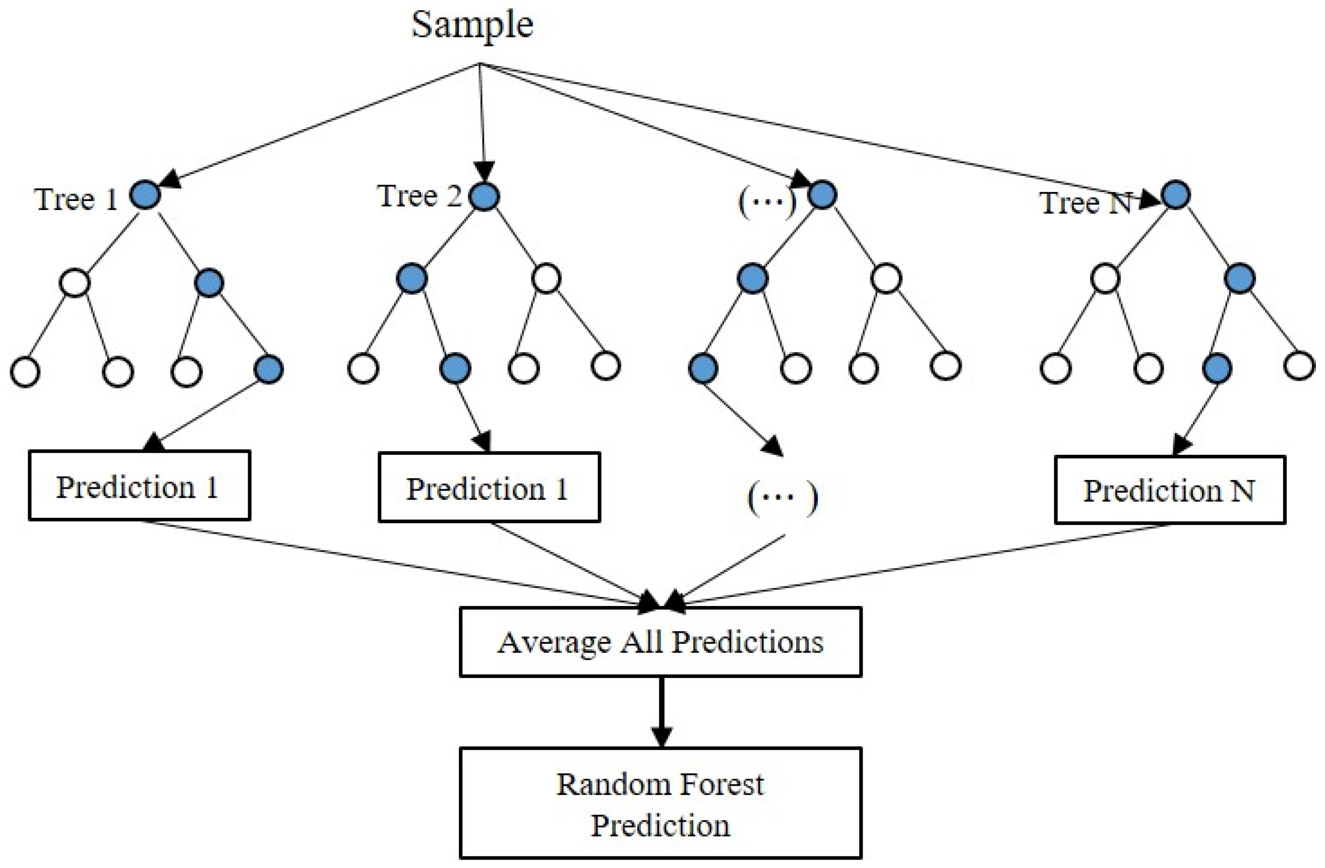
The random forest approach is an improvement of the Bagging ensemble method, which combines the predictions of a group of decision trees. The trees in random forests are run in parallel. There is no interaction between these trees while building the trees. Figure 11 shows the general structure of a random forest. It operates by constructing a multitude of decision trees at training time and outputting the class that is the mode of the classes (classification) or mean prediction (regression) of the individual trees.

To get a better understanding of the random forest algorithm, let us walk through the steps:

• Step 1: Pick at random k data points from the training set.
• Step 2: Build a decision tree associated to these k data points.
• Step 3: Choose the number N of trees you want to build and repeat steps 1 and 2.
• Step 4: For a new data point, make each one of your N-tree trees predict the value of a response variable for the data point in question and assign the new data point to the average across all of the predicted value of response variable.

A random forest regression model is powerful and accurate. It usually performs great on many problems, including features with non-linear relationships. Disadvantages, however, include the following: there is no interpretability, overfitting may easily occur, and we must choose the number of trees to include in the model.

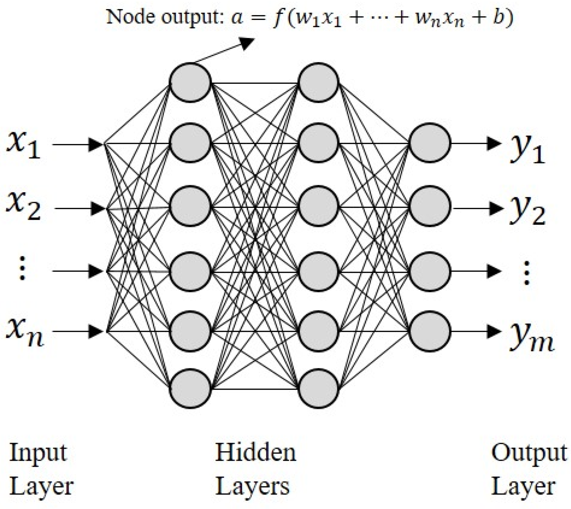
A multi-layer perceptron (MLP) neural network is literally a network composed of multiple layers, and is composed of an input layer, hidden layer, and output layer as shown in the following structure as shown in Figure 12.

If we look at the operation process of MLP in detail, it appears in the following order.

• Step 1: Each data input from the input layer is weighted through each node and the weight that connects the nodes.
• Step 2: It is transformed through the activation function and transferred to the input value (z) of the hidden layer. At this time, ‘Logistic sigmoid unit’ or ‘tanh unit’ is mainly used as the activation function existing in the hidden layer.
• Step 3: In the same way, it is weighted through the weight connected to the output layer, and finally converted and output through the activation function. At this time, the activation function is output as it is in the case of regression, and in the case of binary classification with two-classes of 0 and 1, sigmoid units and the softmax function are met in the case of multi-class.

3.2.5. Pseudocode for Our Proposed Method

The following Algorithm 1 represents the pseudocode for the Korean cattle weight prediction algorithm mentioned above.

Algorithm 1:Procedure Korean Cattle Weight Prediction:

InputRGB-D image and weights.

Fork = 1 to images do 1. Segmentation  % Applying a threshold value to the depth image considering the height of Korean cattle.  $\mathrm{if} D_k>T{H}_1 \&\& D_k<T{H}_2$ then  $D_k^b=255$ ;  $\mathrm{else} D_k^b=0$ ;  % Korean cattle image segmentation using HSI color.  $\mathrm{if} H_k>T{H}_1 \&\& H_k<T{H}_2$ then  $H_k^b=255$ ;  $\mathrm{else} H_k^b=0$ ;  % Create a binarized image by AND-combining the segmented image using depth and color.  $S_k=D_k^b \& H_k^b$ ;  2. Feature Extraction  Find contour for $S_k$  Calculate the central moment about the contour to find the center and rotation angle of Korean cattle.  Apply Affine transformation to adjust the posture of Korean cattle.  Crop cattle area.  % Compute vertical projection profile to remove Korean cattle head.  for j = 1 to width do  $P\left(j\right)=0$;  for i = 0 to height do  if C(i, j) > 0 then  P(j) += 1;  end if  end for  end for  Calculate Body measurement parameters for cropped region.  Calculate Size, Shape, Gradient-based descriptors.  Creating feature vectors using body measures and descriptors. End for 3. Weight Prediction Split feature vectors and Korean cattle weights for training and testing. Training several regression models.

OutputPredicted weight of Korean cattle using testing data.

4. Experiments and Results

4.1. Materials and Interpretation

Here, we conducted an experiment to predict the weight of Korean cattle by dividing the collected dataset into three groups: the combined group, the male group and the female group. The reason for partitioning the groups in this way is that the characteristics of Korean cattle show a large difference between males and females, and the purpose of this study is to examine the characteristics of Korean cattle as a whole. We collected a total of 353 images of 184 male and 169 female images from a total of 15 Korean cattle at 2-week intervals from 22 June 2021 to 17 August 2021. In addition, we constructed data by manually measuring the weight of Korean cattle corresponding to the collected images. In the case of males, Korean cattle weighing approximately 410 to 530 kg in the intermediate growth stage were measured, and in the case of females, young Korean cattle weighing 130 to 210 kg were measured.

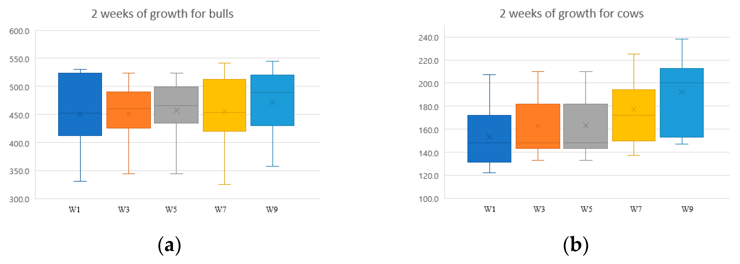
We drew a box plot for measured weights to find out how the weight of Korean cattle for each group grew with time during the period in which the images were collected. Figure 13 shows a box plot of the weights of males and females of Korean cattle at each growth stage. From the given box plot, we can see that the weights of males and females gradually increase according to the observation period, and in particular, in the case of females, the relative weight increase rate is slightly faster than that of males. This result is thought to be due to the fact that young calves generally grow faster than intermediate stage Korean cattle because females were used for young Korean cattle and males for intermediate stage Korean cattle.

4.2. Experimental Results

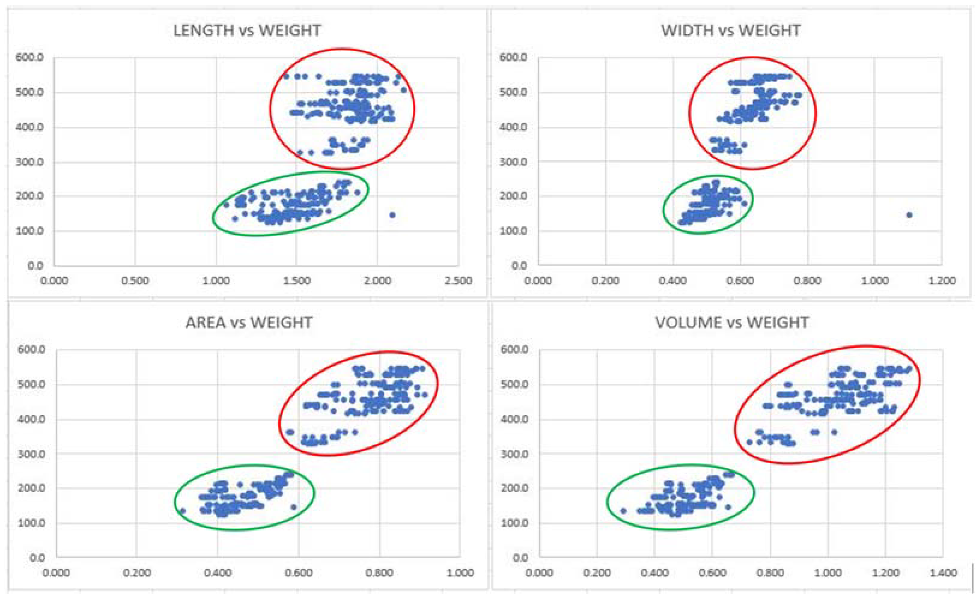
First, we examined the relationship between four body characteristics and body weight for male and female Korean cattle groups using training data. Figure 14 shows the relationship between the extracted four body characteristics and the weight of Korean cattle using a scatter plot. From the given scatter plot, we found that the most suitable order of body measurements to predict the weight of Korean cattle was volume, area, length, and chest height.

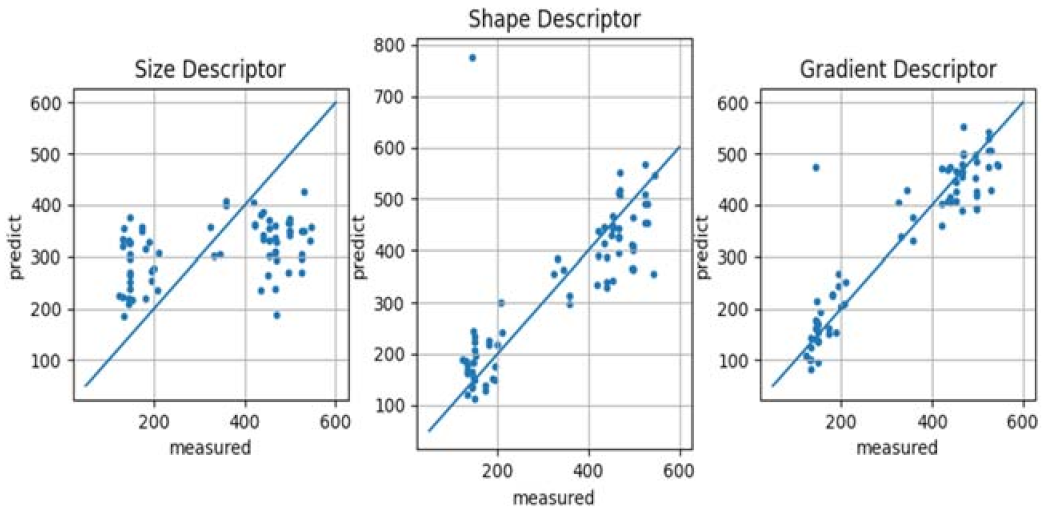
Second, the effect of the three proposed shape descriptors on predicting the weight of Korean cattle was examined. To confirm this, we performed multiple regression analysis on each descriptor and weight, and produced a scatter plot of the actual and predicted values. Figure 15 shows a scatter plot of predicted values and actual observations using three types of descriptors. From the given results, we can see that among the three types of descriptors, the gradient-based descriptor predicts the weight of Korean cattle best, followed by the shape descriptor generally well. However, it was found that the size descriptor did not express the weight of Korean cattle well in general. The cause of this problem seems to be that the change in the size of Korean cattle is not large due to the short growth period.

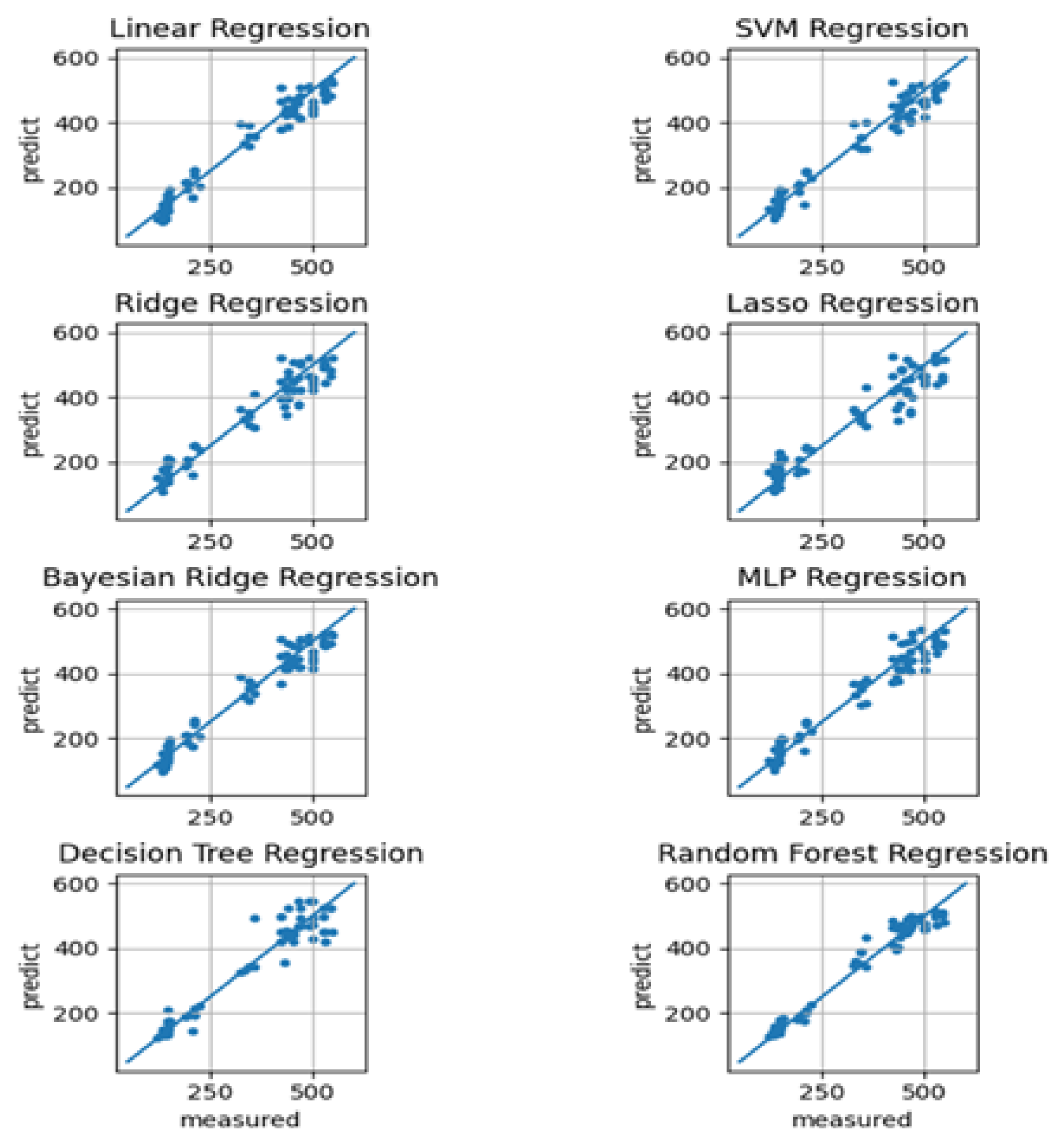
Third, we conducted an experiment comparing the performance of eight predictive models based on the extracted 34-dimensional feature vectors. Figure 16 shows a scatter plot of the actual observed and predicted values of Korean cattle predicted by applying various regression models using 34-dimensional feature vectors as explanatory variables based on the total collected data. From Figure 16, we can see that most of the eight prediction methods predict the weight of Korean cattle well. Among them, the model with the best predictive power is random forest, and it can be seen that linear regression and decision trees are given in order.

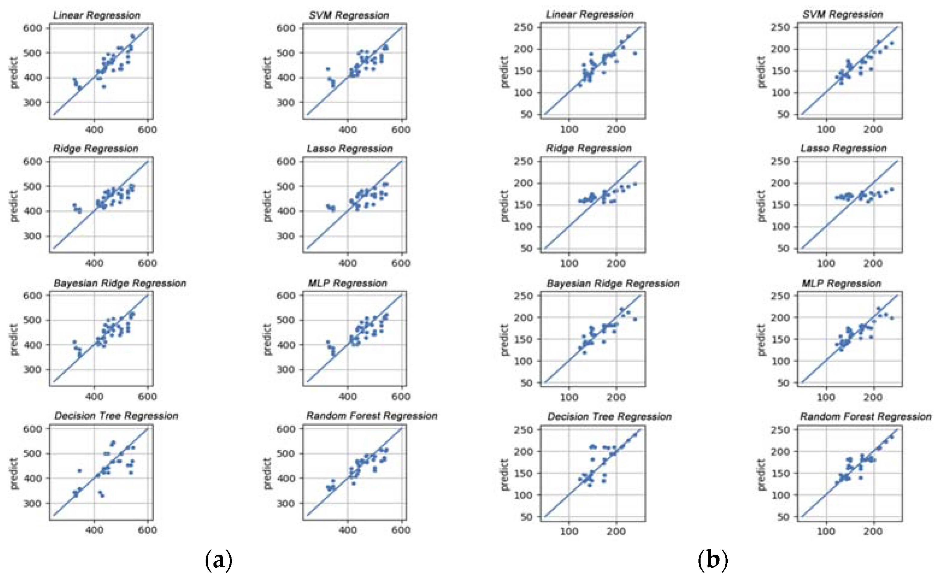
In addition, Figure 17 shows a scatterplot prepared using the results obtained by applying the same method by dividing the collected Hanwoo data into male and female groups. From a given results, we can see that the accuracy of most prediction models is generally lowered when the entire data is divided into male and female groups for prediction. In particular, the models with the lowest accuracy among them were ridge, LASSO, and decision tree. The reason for this result is that, firstly, there is not much data used for each divided group and, secondly, the change in body weight does not appear to be significant due to the short growth period. However, despite the lack of training data, models such as linear regression, random forest, and Bayesian ridge regression showed relatively good predictive power for both males and females.

Fourth, we calculated the coefficient of determination to numerically evaluate the predictive power of eight nonlinear regression and machine learning models of Korean cattle weight.

Table 1. Show the coefficient of determination.

Method	Coefficient of Determination (R2)
	Total (Male + Female)	Male	Female
Linear Regression	0.955500	0.718056	0.658056
SVM Regression	0.947167	0.655915	0.735438
Ridge	0.924378	0.559549	0.402620
LASSO	0.905019	0.485137	0.070050
Bayesian Ridge	0.955736	0.697338	0.717989
MLP	0.941887	0.667934	0.705792
Decision Tree	0.936354	0.464219	0.279362
Random Forest	0.968880	0.755998	0.732490

shows the coefficients of determination of the eight models for the entire group and each of the male and female groups. From the given Table 1, linear regression, SVM, Bayesian ridge regression, and random forest regression models show a high coefficient of determination in the entire group or both sexes. Therefore, these models seem to have the best predictive power in predicting the weight of Korean cattle. It can be seen that these results are generally consistent with the results discussed through the scatter plot above.

Finally, we calculated the MSE measure to numerically compare the predictive power of various machine learning methods. The

Table 2. Show the mean square error.

Method	Mean Square Error
	Total (Male + Female)	Male	Female
Linear Regression	1051.7	1108.5	300.6
SVM Regression	1248.5	1352.8	232.6
Ridge	1787.1	1731.7	525.2
LASSO	2244.5	2024.3	817.6
Bayesian Ridge	1046.0	1190.0	247.9
MLP	1373.3	1305.6	258.6
Decision Tree	1504.0	1973.9	663.4
Random Forest	735.4	959.3	235.2

shows the MSE values of various machine learning methods for the entire population and for both male and female cattle. From the given Table 2, we can see that the random forest has the smallest mean square error among various machine learning methods, followed by Bayesian ridge, linear regression, and SVM regression in the order of the mean square error.

The meaning of total shown in Table 1 and Table 2 means adding all the data of male and female cattle. For the experiment, we analyzed each of the three groups: a female group, a male group, and a total group combining the two groups. The reason for this is that, in the case of Hanwoo, the weight gain of males differs from that of females during the rearing period, so these groups were analyzed separately. Moreover, the coefficient of determination we used is an index indicating how well the hypothesized regression model can explain the weight prediction. The value of this index may appear differently depending on the uniformity and size of the observed data. Therefore, the reason that each coefficient of determination for the female and male groups was smaller than the coefficient of determination for the total group appears to have occurred because the weight increase rate of males and females during the growth period of Korean cattle is different and the number of data collected is not large. However, looking at the experimental results, it can be seen that the top three predictive models of female, male, and total data show a high coefficient of determination regardless of whether female, male, and total individuals are classified.

5. Conclusions

In this paper, we proposed an automatic weight prediction system for Korean cattle using the Bayesian ridge algorithm on an RGB-D image. The proposed system consists of three parts: segmentation, extraction of features, and estimation of the weight of Korean cattle from a given RGB-D image. The first step is to segment the Hanwoo area from a given RGB-D image using depth information and color information, respectively, and then combine them to perform optimal segmentation. Additionally, we correct the posture using ellipse fitting on segmented body image. The second step is to extract features for weight prediction from the segmented Hanwoo image. We extracted three features: size, shape, and gradients. The third step is to find the optimal machine learning model by comparing eight types of well-known machine learning models. In this step, we compared each model with the aim of finding an efficient model that is lightweight and can be used in an embedded system in the real field. To evaluate the performance of the proposed weight prediction system, we collected 353 RGB-D images from livestock farms in Wonju, Gangwon-do in Korea. In the experimental results, random forest showed the best performance, and the Bayesian ridge model is the 2nd best in MSE or the coefficient of determination. However, we believe that the Bayesian ridge model is the most optimal model in the aspect of time complexity and space complexity. Finally, it is expected that the proposed system will be casually used to determine the shipping time of Hanwoo in wild farms for portable commercial devices. We also hope to use more sensors, but it is not easy to attach and measure many sensors to live animals in the field and synchronize the collected data. Therefore, as the miniaturization of sensors and the convenience of data collection increase in the future, we plan to develop a more accurate prediction model by conducting continuous experiments.

References

- Silvia, L.-C.; Rodolfo, R.V.A.; Gilberto, A.-O.A.; María, E.O.-C.B.; Juan, C.G.-O. Stress indicators in cattle in response to loading, transport and unloading practices. Rev. Mex. Cienc. Pecu. 2019, 10, 885–902. [Google Scholar] [CrossRef] [Green Version]
- Insaf, A.; Abdeldjalil, O.; Amir, B.; Abdelmalik, T.A. Past, Present, and Future of Face Recognition: A Review. Electronics 2020, 9, 1188. [Google Scholar] [CrossRef]
- Yacine, K.; Amir, B.; Abdeldjalil, O.; Sébastien, J.; Abdelmalik, T.-A. Ear Recognition Based on Deep Unsupervised Active Learning. IEEE Sens. J. 2021, 21, 20704–20713. [Google Scholar] [CrossRef]
- Bultakov, K.; Kim, Y.C.; Lee, H.M.; Na, I.S. A BPR-CNN Based Hand Motion Classifier Using Electric Field Sensors. CMC-Comput. Mater. Contin. 2022, 71, 5413–5425. [Google Scholar]
- Do, L.N.; Yang, H.J.; Nguyen, H.D.; Kim, S.H.; Lee, G.S.; Na, I.S. Deep neural network-based fusion model for emotion recognition using visual data. J. Supercomput. 2021, 77, 10773–10790. [Google Scholar] [CrossRef]
- Cho, W.H.; Kim, S.K.; Na, M.H.; Na, I.S. Fruit Ripeness Prediction Based on DNN Feature Induction from Sparse Dataset. CMC-Comput. Mater. Contin. 2021, 69, 4003–4024. [Google Scholar]
- Lee, K.O.; Lee, M.K.; Na, I.S. Predicting Regional Outbreaks of Hepatitis A Using 3D LSTM and Open Data in Korea. Electronics 2021, 10, 2668. [Google Scholar] [CrossRef]
- Cho, W.H.; Kim, S.K.; Na, M.H.; Na, I.S. Forecasting of Tomato Yields Using Attention-Based LSTM Network and ARMA Model. Electronics 2021, 10, 1576. [Google Scholar] [CrossRef]
- Chang, Y.; He, H.; Qiao, Y. An Intelligent Pig Weights Estimate Method Based on Deep Learning in Sow Stall Environments. IEEE Access 2019, 7, 164867–164875. [Google Scholar] [CrossRef]
- Femandes, A.F.A.; Dorea, J.R.R.; Rosa, G.J.M. Image Analysis and Computer Vision Applications in Animal Sciences: An Overview. Front. Vet. Sci. 2020, 7, 551269. [Google Scholar] [CrossRef]
- Nasirahmadi, A.; Edwards, S.A.; Sturm, B. Implementation of machine vision for detecting behavior of cattle and pigs. Livest. Sci. 2017, 202, 25–38. [Google Scholar] [CrossRef] [Green Version]
- Wang, Z.; Shadpour, S.; Chan, E.; Rotobdo, V.; Wood, K.M.; Tulpan, D. ASAS-NANP SYMPOSIUM: Application of machine learning for livestock body weight prediction from digital images. J. Anim. Sci. 2021, 99, skab022. [Google Scholar] [CrossRef] [PubMed]
- Seo, K.-W.; Lee, D.-W.; Choi, E.-G.; Kim, C.-H.; Kim, H.-T. Algorithm for Measurement of the Dairy Cow’s Body Parameters by Using Image Processing. J. Biosyst. Eng. 2012, 37, 122–129. [Google Scholar] [CrossRef] [Green Version]
- Tasdemir, S.; Ozkan, İ.A. Ann Approach for Estimation of Cow Weight Depending on Photogrammetric Body Dimensions. Int. J. Eng. Geosci. 2019, 4, 36–44. [Google Scholar] [CrossRef]
- Huang, L.; Guo, H.; Rao, Q.; Hou, Z.; Li, S.; Qiu, S.; Fan, X.; Wang, H. Body Dimension Measurements of Qinchuan Cattle with Transfer Learning from LiDAR Sensing. Sensors 2019, 19, 5046. [Google Scholar] [CrossRef] [PubMed] [Green Version]
- Rudenko, O.; Megel, Y.; Bezsonov, O.; Rybalka, A. Cattle breed identification and live weight evaluation on the basis of machine learning and computer vision. In Proceedings of the Third International Workshop on Computer Modeling and Intelligent Systems (CMIS-2020), CMIS-2020 Computer Modeling and Intelligent Systems, Zaporizhzhia, Ukraine, 27 April–1 May 2020; pp. 939–954. [Google Scholar]
- Pradana, Z.H.; Hidayat, B.; Darana, S. Beef cattle weight determine by using digital image processing. In Proceedings of the 2016 International Conference on Control, Electronics, Renewable Energy and Communications (ICCEREC), Bandung, Indonesia, 13–15 September 2016; pp. 179–184. [Google Scholar] [CrossRef]
- Weber, V.A.M.; Weber, F.L.; Gomes, R.C.; Oliveira Junor, A.S.; Menezes, G.V.; Abreu, U.G.P.; Belete, N.A.S.; Pistori, H. Prediction of Girolando cattle weight by means of body measurements extracted from images. Rev. Bras. Zootec. 2020, 49, e20190110. [Google Scholar] [CrossRef] [Green Version]
- Gjergji, M.; de Weber, V.M.; Silva, L.O.C.; da Gomes, R.C.; de Araujo, T.L.A.C.; Pistori, H.; Alvarez, M. Deep Learning Techniques for Beef Cattle Body Weight Prediction. In Proceedings of the International Joint Conference on Neural Networks (IJCNN), Glasgow, UK, 19–24 July 2020; pp. 1–8. [Google Scholar]
- Rodríguez, A.J.; Arroqui, M.; Mangudo, P.; Toloza, J.; Jatip, D.; Rodriguez, J.M.; Teyseyre, A.; Sanz, C.; Zunino, A.; Machado, C.; et al. Estimating Body Condition Score in Dairy Cows from Depth Images Using Convolutional Neural Networks, Transfer Learning and Model Ensembling Techniques. Agronomy 2019, 9, 90. [Google Scholar] [CrossRef] [Green Version]
- Lee, D.H.; Lee, S.H.; Cho, B.K.; Wakholi, C.; Seo, Y.W.; Cho, S.H.; Kang, T.H.; Lee, W.H. Estimation of carcass weight of Hanwoo (Korean native cattle) as a function of body measurements using statistical models and a neural network. Asian-Australas. J. Anim. Sci. 2020, 33, 1633–1641. [Google Scholar] [CrossRef] [Green Version]
- Jang, D.H.; Kim, C.; Ko, Y.-G.; Kim, Y.H. Estimation of Body Weight for Korean Cattle Using Three-Dimensional Image. J. Biosyst. Eng. 2020, 45, 325–332. [Google Scholar] [CrossRef]
- Lee, S.U.; Chung, S.Y.; Park, R.H. A comparative performance study of several global thresholding techniques for segmentation. Comput. Vis. Graph. Image Process. 1990, 52, 171–190. [Google Scholar] [CrossRef]
- Liu, Z.; Zhao, C.C.; Wu, X.M.; Chen, W.H. An Effective 3D Shape Descriptor for Object Recognition with RGB-D Sensors. Sensors 2017, 17, 451. [Google Scholar] [CrossRef] [PubMed] [Green Version]
Figure 1.
Sample images for male and female Korean cattle: (a) male; (b) female.
Figure 2.
Overview of prediction system for cattle weight.
Figure 3.
Segmentation process of cattle from depth image. (a) Depth image of cattle. (b) Histogram of depth image. (c) Segmentation result of cattle.
Figure 4.
Segmentation process of cattle from RGB image: (a) Hue component of cattle; (b) histogram of Hue image; (c) segmentation result of cattle.
Figure 5.
Final segmentation result of cattle in RGB-D image.
Figure 6.
3D segmented cattle image and its bounding box.
Figure 7.
Correcting the posture of Korean cattle using ellipse fitting.
Figure 8.
Show the point cloud data within a specific area: (a) segmented cattle image; (b) 3D coordinates for pixels in box region.
Figure 9.
Process of calculating the length and width of Korean cattle.
Figure 10.
Three kernel shape descriptors derived from Korean cattle image.
Figure 11.
The general structure of a random forest.
Figure 12.
Structure of multilayer perceptron.
Figure 13.
Boxplot for growth cattle weight of males and females: (a) male cattle; (b) female cattle.
Figure 14.
Scatter plot of the relationship between the four body characteristics and the cattle weight: red circle is male; green circle is female.
Figure 15.
Scatter plot for the actual value and predicted value using three kinds of descriptors.
Figure 16.
Scatterplot between predicted value and measured value for total (male and female) dataset.
Figure 17.
Scatterplot between predicted value and measured value for male and female dataset: (a) male; (b) female.