Monitoring System for the Management of the Common Agricultural Policy Using Machine Learning and Remote Sensing

Abstract

The European Commission promotes new technologies and data generated by the Copernicus Programme. These technologies are intended to improve the management of the Common Agricultural Policy aid, implement new monitoring controls to replace on-the-spot checks, and apply up to 100% of the applications continuously for an agricultural year. This paper presents a generic methodology developed for implementing monitoring controls. To achieve this, the dataset provided by the Sentinel-2 time series is transformed into information through the combination of classifications with machine learning using random forest and remote sensing-based biophysical indices. This work focuses on monitoring the helpline associated with rice cultivation, using 13 Sentinel-2 images whose grouping and characteristics change depending on the event or landmark being sought. Moreover, the functionality to check, before harvesting the crop, that the area declared is equal to the area cultivated is added. The 2020 results are around 96% for most of the metrics analysed, demonstrating the potential of Sentinel-2 for controlling subsidies, particularly for rice. After the quality assessment, the hit rate is 98%. The methodology is transformed into a tool for regular use to improve decision making by determining which declarants comply with the crop-specific aid obligations, contributing to optimising the administrations’ resources and a fairer distribution of funds.

1. Introduction

The main objective of the new European Common Agricultural Policy (CAP) (EU Regulation No. 1307/2013) is the development of favourable and sustainable actions to promote efficient agricultural practices. To this end, they must ensure food security, provide raw materials to the agri-food industries, and generate benefits for a sustainable and competitive agricultural sector [1]. To achieve these objectives, the European Commission supports the implementation and use of new technologies to achieve simplification of the implementation and management of CAP support. Furthermore, with the revision made by the Commission Implementing Regulation (EU Regulation 2018/746), remote sensing-based methodologies have become an effective mechanism for agricultural monitoring and management. In this respect, monitoring controls play an important role as the primary control methodology to be applied during the period of the new CAP reform to area-based interventions, replacing classical on-the-spot checks. Monitoring controls are a procedure of periodic and systematic observation of the earth, based mainly on satellite images. These checks are preventive, and their objective is the regular and continuous verification of the compatibility between the agricultural activity declared by the farmer and that is observed in the time series through the use of satellite images [2]. This information, processed with artificial intelligence systems and remote sensing techniques, allows automatic verification of the criteria for aid eligibility. In addition, the automation of processes tends to reduce the administrative burden and the cost of carrying out CAP aid controls, thus making the processing of applications and payments more agile.

In this sense, the aerospace sector plays a fundamental role, thanks to the Copernicus Programme, developed by the European Union, the most ambitious Earth observation programme in history. It is designed to provide accurate, up-to-date, and easily accessible information to improve environmental management and mitigate the effects of climate change, among its many applications. The information generated in the framework of the Copernicus Programme is obtained by the observations of different satellite missions called Sentinel, which, together with measurement data on land, sea, and air, allow the use of this information to achieve multiple purposes [3]. The unique characteristics of this type of imagery are its high frequency of data acquisition and its resolution, which make it possible to monitor agricultural areas. These images are beneficial, as they provide public policymakers with relevant, timely, and low-cost information on which to base their decision making, implementation, and monitoring of interventions in the management of agricultural aid.

In the agri-food sector, artificial intelligence (AI) has been deployed to achieve better crop production, disease prediction, continuous monitoring, improved operational efficiency, and optimised water management. To design quality control methodologies and the ability to reach and serve society at the lowest possible cost, machine learning (ML) and deep learning are two of the most widely used approaches. Individuals, businesses, and government agencies use these models to anticipate and learn from data. The incorporation of ML opens up new possibilities for obtaining mathematical models and making highly accurate predictions of different agronomic variables and the evolution of crops. In addition, the use of ML, together with the help of remote sensing-based techniques, enables improved decision making in agriculture so that a horizon, where efficiency, increased profitability, and sustainability at a lower cost become a reality, is foreseen [4].

Using AI and remote sensing technologies makes it possible to improve agriculture-related tasks and improve decision making by monitoring farms in real time. There is currently a wide variety of methods for detecting crop yield estimation based on various data and remote sensing techniques. Some work aims to assess the potential of combining vegetation spectral information with ground spectral information for crop monitoring using satellite (Worldview 2/3) and UAV data fusion, together with ML algorithms [5]. Other works make use of the image repository provided by the Copernicus Programme to develop automated methods for winter crop monitoring using time series of Sentinel-2 (S2) images [6]. In the literature, we find different works that make use of S2 images to improve agricultural decision making: to enhance precision agriculture by focusing on the spatial, spectral, and temporal resolution of the images [7], to classify fallow land in the arid Sahelian region [8], or as a tool to evaluate the use of vegetation indices over several years to calculate the nitrogen uptake of crops [9].

Based on the work published by López-Andreu et al. [10], which proposes a methodology to identify rice cultivation by ML, using S2 data, in this work, the methodology developed in that article is improved by confronting the results obtained in the extraction of biophysical index signals, the random forest (RF) classification of a multi-element time series, and the RF classification of a single S2 image. In addition, a detailed treatment of the resulting RF classification rasters is added to discover whether 100% of the area declared in the aid application (toward the end of the crop’s vegetative development) is cultivated. Finally, all the data are entered, with specific weights according to the origin, in a decision tree to generate a chromatic indicator. This indicator reflects whether the aid obligations are fulfilled (green), whether these obligations are not fulfilled (red), or whether the system cannot give a conclusive result (yellow).

Finally, it has been possible to develop a decision support tool that, by managing S2 data through traditional remote sensing and RF, allows for continuous analysis, constantly and periodically, throughout the agricultural campaign, under the premise of monitoring compliance with the obligations undertaken by the declarants on the aid line associated with rice. The application of this work contributes to automating and improving the management of aid to bring about a change of approach in the management of CAP aid, with automated mass control and almost no field visits or measurements.

In summary, it was possible to design a methodology that combines the results obtained by three intermediate products, i.e., biophysical indices, RF classification of date, and RF classification of a time series, to determine whether the obligations of the rice aid were being met with up to 97% effectiveness. The time series RF classification showed the most significant specific weight in the final performance. However, it was clear that the combination of all intermediate products was instrumental in minimising errors, resulting in a better and fairer distribution of CAP resources. This methodology contributed to detecting 12 fraudulent aid applications, representing 4% of the total number of applications monitored. The process was carried out continuously on 100% of the aid applications for the agricultural year without any field visits.

2. Related Work

Today, different research projects promote the use of AI, of which we highlight the following: NaLamKI [11], which aims to promote more efficient and sustainable agriculture by developing artificial intelligence methods to analyse remote sensing data for modelling agricultural processes and for 5G networks on farms, or knowlEdge [12], which proposes, among other things, a knowledge-based platform to distribute and exchange trained AI models. Other, more concrete, examples allow us to solve needs in the agricultural sector: reducing the environmental impact of pesticides in pest management [13] or controlling the artificial lighting system to optimise the energy efficiency of greenhouses [14].

Currently, several studies use satellite images for crop identification, which serve as a helpful tool for managing the different CAP campaigns. The work carried out by Sarvia, F. et al. [15] was based on the classification of the Normalised Difference Vegetation Index (NDVI) time series of S2 using supervised classification algorithms (minimum distance and random forest) in the province of Vercelli (Northwest Italy). Siesto, G. et al. [16] presented a novel crop identification approach by applying neural networks with multiple satellite images using synthetic inputs at a pixel level. Moreover, crops that were abandoned and did not qualify for the CAP basic payment were detected. In the work of Portalés-Julià, E. et al. [17], such plots in the province of Valencia (Spain) were determined by evaluating time series of S2-derived spectral indices, together with machine learning and deep learning algorithms, to discriminate abandoned plots.

Different works have addressed the detection of rice cultivation using satellite imagery. Hedayati et al. combined rice phenology and an object-based classification method using Landsat-8 image series, MODIS sensor temperature data, and a digital terrain elevation model. Ramadhani et al. [18] used different Sentinel (1 and 2) and MODIS data sources combined with the support vector machine classification method to generate a multi-temporal rice map. Moreover, rice was monitored using synthetic aperture radar-based solutions that are immune to rainfall and clouds, as proposed by Chang et al. [19]. The use of time series of S2 images combined with the help of different vegetation indices allowed the quantification of the rice yield in each of its phenological stages, as proposed by Nazir et al. [20]. Sitokonstantinou et al. [21] implemented a complete line for rice mapping at massive scales and high spatial resolution, using a distributed RF classifier that was trained with pseudo-labels on a time series of Sentinel image data.

A major constraint in rice crop monitoring for the management of CAP subsidies is the mandatory use of Sentinel imagery, which makes using other satellites impossible. The combination of RF classification for a time series and a specific date increases the accuracy from 95% to 97%, which may not be considered a significant improvement. However, it is associated with generating a more efficient aid distribution from European funds, representing considerable savings. The use of deep learning was not considered, as 97% accuracy was deemed sufficient to determine fraudulent applications.

3. Study Area

After choosing rice as the crop to be identified through the defined methodology, one of Spain’s most important producing areas was selected. The municipality of Calasparra (Coordinates: 38.13, −1.42) is located in the northwest of the Region of Murcia (Spain) and is known for its rice (especially the Bomba variety), which has the Denomination of Origin Calasparra Rice [22], the rice reserve being delimited by three municipalities: Calasparra, Moratalla (Murcia Region), and Hellín (Autonomous Community of Castilla-La Mancha).

This work focused on the 2020 crop year, which had 64 registered dossiers, representing a total of 324 declaration lines associated with rice cultivation, with around 340 hectares declared. Figure 1 shows the different plots that form part of the declared lines under study.

Contrary to what may occur in other areas, due to the orography of the terrain, in the study area, we find plots of small dimensions whose shape is heterogeneous. In

Table 1. Typology of the study enclosures according to their surface area.

Total Plots	Size (Hectares)
146	≤0.5
223	≤1
55	1 ≤ x ≤ 2
7	≥5

, the relationship between the number of plots and the range of surface area is specified.

Finally, it should be noted that vegetables and leguminous plants are usually grown in the study area, a circumstance which, together with the shape and layout of the plots and the spatial resolution of the S2 images, complicates the identification of rice cultivation.

4. Materials and Methods

4.1. Materials

The materials used come from three different sources: information on rice cultivation and farming practices, satellite image data, and vector data.

For the development of the implemented system, tools based on free software were used. Python libraries, such as rasterio, shapely, or rasterstats were used for GIS data processing, and the Python scikit-learn library was used for ML functionality. A PostgreSQL database with its PostGIS spatial extension was used to store the data. To access the S2 image repository, the Python requests library and the Copernicus Open Access API Hub [23] were used.

Finally, the implemented tool was deployed on a proprietary server with Windows 2016 Server as the operating system, 64 GB of RAM, 4 TB of hard disk, and an RTX2080Ti graphics card.

4.1.1. Phenological Information

The methodology developed requires information on the different phenological stages of the development of the crop to be identified. With the data obtained from the phases and their cultivation dates, we can locate the phenological stage of the crop [24].

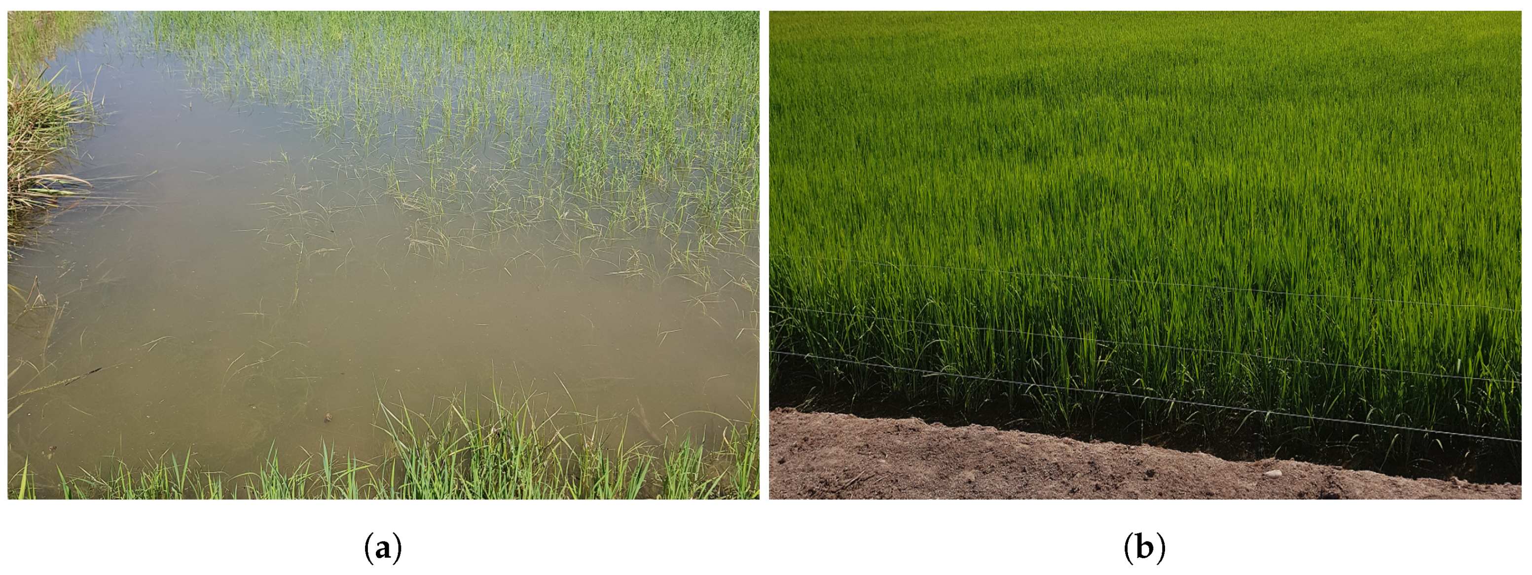
In the specific case of rice cultivation, the previous work showed that two main events allowed us to identify this crop. The first is the flooding of the agricultural plot, which takes place from May to June, and the second is the vigour that the crop reaches during its development between June and August. Figure 2 shows these two events.

4.1.2. Sentinel Data

The Copernicus Programme includes the Sentinel missions, which are made up of two satellites to provide an ideal coverage and observation frequency to offer a robust data set. There are five Sentinel missions [25], although only Sentinel-1 (S1) and S2 focus on ground monitoring. S1 provides radar imagery, while S2 provides optical imagery [26].

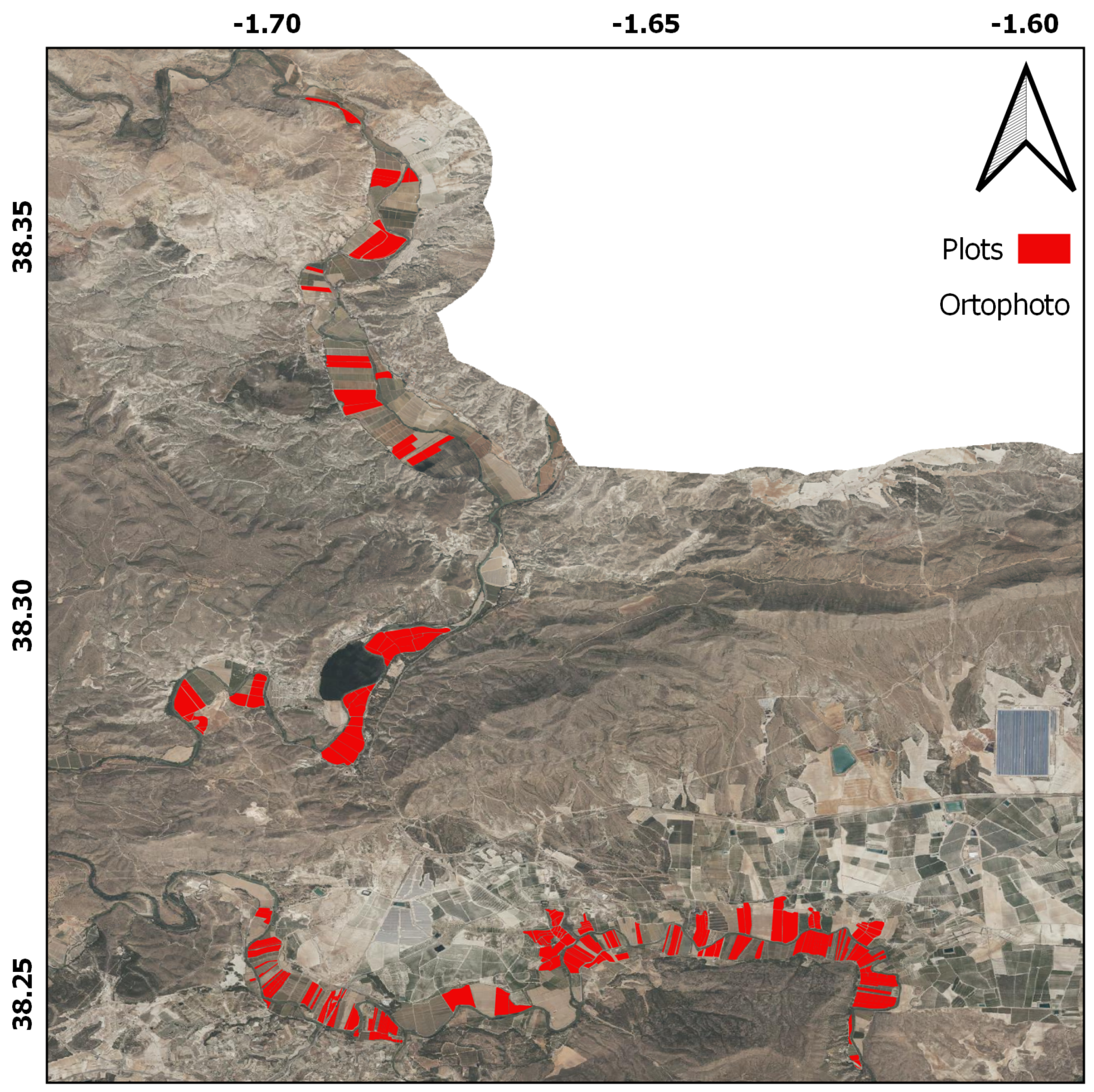
Due to the low cloud cover and the temporal resolution (5 days) offered by S2, it was considered that these data are sufficient for this work, so the use of S1 was discarded. The study area is entirely covered by orbit number 051, and the S2 tessera T30SXH is in the EPSG:32630 reference system.

The previously published work concluded that monitoring agricultural plots outside the crop development period did not provide additional accuracy to the model. Therefore, concerning the satellite images, this work focused on the period where crop development was most noticeable, based on the phenological information. For this reason, there was a time series of 13 elements from 20 May 2020 to 28 August 2020, both dates inclusive.

All the elements of this time series had a 0% cloud cover. S2 carries a multispectral instrument (MSI), which is defined as a high-resolution wide-band multispectral imaging system operating in 13 spectral bands at multiple spatial resolutions. The product used was the so-called S2MSI2A, whose main features are level 2A processing, orthorectification, and UTM geocoding, BOA, and multispectral reflectance [27].

The S2 bands used in this work were B2, B3, B4, B8, and B11, because of their spatial resolution and because they are necessary for the generation of level 3 products used as complementary data.

Table 2. Characteristics of the S2 bands used.

Band	Spatial Resolution	Central Wavelength	Description
B2	10 m	490 nm	Blue
B3	10 m	560 nm	Green
B4	10 m	665 nm	Red
B8	10 m	842 nm	Near Infrared (NIR)
B11	20 m	1610 nm	Short-wave Infrared (SWIR)

shows detailed technical information for these bands:

4.1.3. Vectorial Data

The aid declarations of the applicants are mechanised in the aid management system (SGA) application, offered by the Spanish Agricultural Guarantee Fund (FEGA) to the different autonomous communities. The aid declarations entered in the system contain both alphanumeric and spatial information. The spatial information is based on the Geographical Information System of Agricultural Parcels (SIGPAC), although the declarant also can digitise their agricultural parcel. As for the alphanumeric information supplied by the SGA, we can use the identification of the aid line, the applicant, identification of the enclosure, or the type of aid requested.

4.2. Methodology

4.2.1. Overview

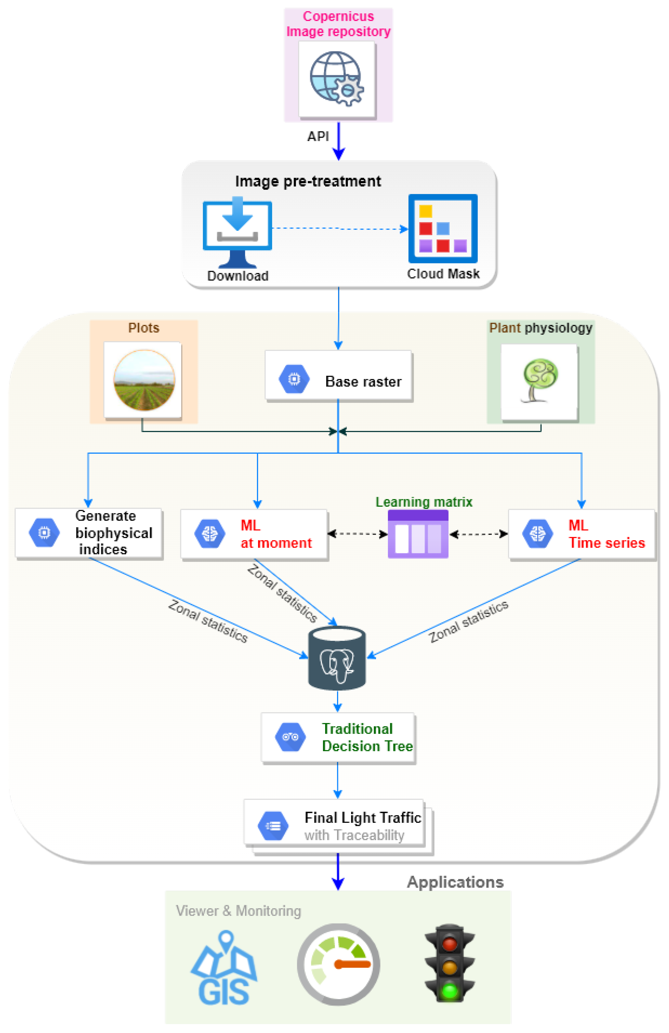
The generic methodology followed to monitor crops, especially rice, using S2 imagery and machine learning and traditional remote sensing techniques to replace the field controls of CAP aid management, follows the scheme presented in Figure 3.

When defining the methodology, the findings of previous studies played an important role, especially the fact that the monitoring of the crop on dates of little relevance did not have a significant final contribution. It should be noted that in the different phenological phases of the crop, only those characteristics were used that would help us to identify the rice crop univocally, thus avoiding the creation of large matrices with data that would probably contribute little value to the final result and introduce uncertainty into the model [28].

Since monitoring must be treated as a continuous process, the methodology used was carried out on 13 occasions, as many times as the number of S2 images available for the area, with zero cloud cover, between the dates when the rice crop was most easily recognizable, either because of agricultural practices or because of its vegetative development, more specifically between May and September.

In short, this work aimed to develop a methodology that would make it possible to identify a crop, specifically rice, continuously, during a complete agricultural campaign, using classical remote sensing and RF classification with satellite data and, in addition, to discern whether the principle of cardinality was met, which implies that 100% of the area declared in the aid application was cultivated.

4.2.2. Sentinel-2 Repository

A process was implemented in which, using the Copernicus Hub API, connected to the Hub, and, for a specific date, using the scene classification map (SCL) of the T30SXH scene, the cloud cover over the study area was checked. If the cloud cover in the area was zero, a raster of the study area was generated using the bands indicated in Table 2. After applying a clipping operation with the study area, the resulting raster had a size of 1538 rows and 1003 columns with a total of 1,542,614 pixels.

4.2.3. Biophysical Indices

Using as input the raster generated in the previous point, the plot with the geometries of the aid declarations, and the phenological characteristics of the crop, we proceeded with the creation of the most representative biophysical index, according to the stage of development of the crop in which we found ourselves.

The NDVI index is widely used to estimate the quantity, quality, and development of vegetation based on measuring the intensity of radiation from certain bands of the electromagnetic spectrum that vegetation emits or reflects. It normalises the scattering of green leaves at near-infrared wavelengths (S2 band 8) with chlorophyll absorption at red wavelengths (S2 band 4). It ranges in value from −1 to 1. Negative values close to −1 correspond to water, and values close to zero usually correspond to arid areas. Values between 0.2 and 0.4 typically represent shrubs and grasslands, while high values represent living green vegetation.

The NDVI [29] index was used for the initial non-crop stage and the growth phase and is defined as

$$NDVI=\frac{B8-B4}{B8+B4}$$

(1)

The Normalised Difference Water Index (NDWI) index is used for the detection of water bodies. These water bodies absorb light in the visible to infrared electromagnetic spectrum (S2 band 8); the NDWI uses the green band (S2 band 3) and near-infrared to highlight water bodies. Near-infrared minimises the low reflectance for water features and maximises the high reflectance for terrestrial vegetation and soils, while green maximises the reflectance of water features.

The NDWI Index [30] for the flooding phase of the agricultural plots is defined as

$$NDWI=\frac{B3-B8}{B3+B8}$$

(2)

Values higher than −0.2 correspond to water bodies flooding the crop plots in the study area.

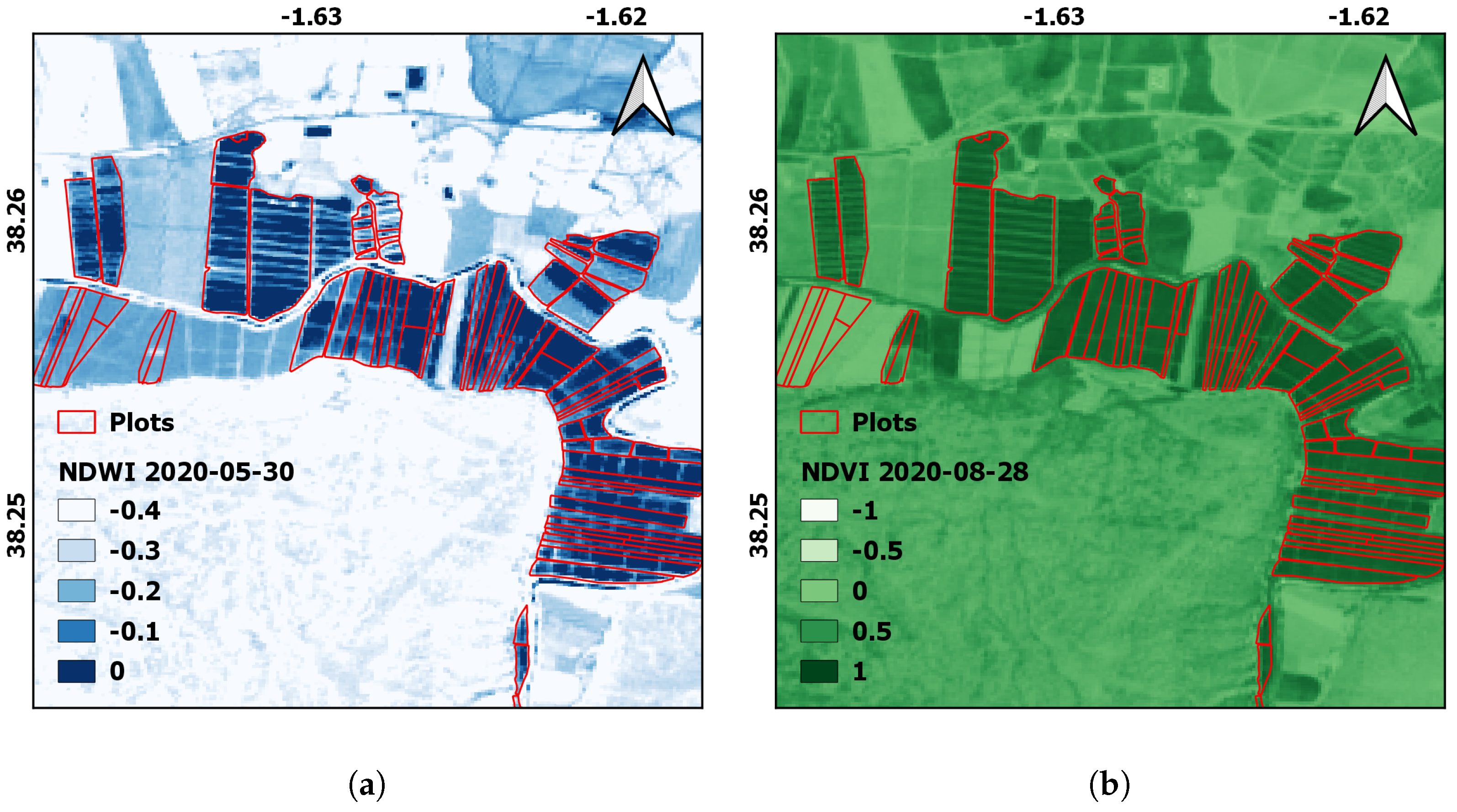
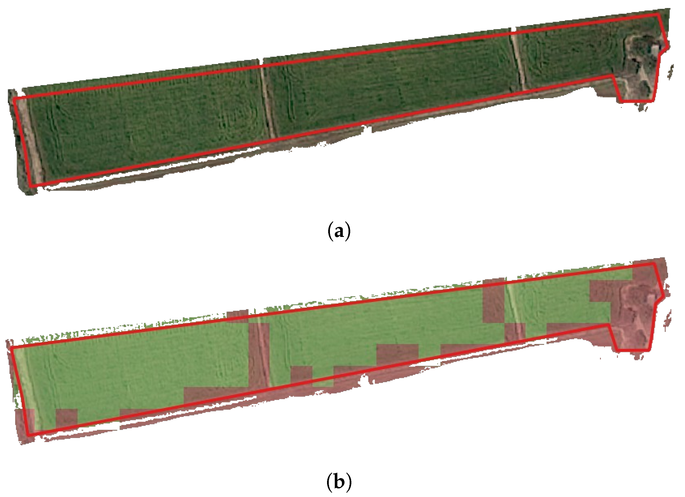
Figure 4 shows how the NDWI index highlights flooded plots and how the NDVI index highlights plots with optimal vegetative development.

With the resulting raster and the geometries of the parcel with the aid applications, a zonal statistic was carried out, obtaining a series of basic statistics, such as mean, standard deviation, or number of pixels, which were finally stored in the database generated for this work for subsequent processing.

4.2.4. Learning Matrix for Classifications by Machine Learning

The learning matrix used contains elements of two classes; code 80 to identify the rice crop and code 1 for any other crop or type of surface.

The samples were generated using information obtained from field visits and the photo interpretation of a Pleiades-1 image with a spatial resolution of 50 centimetres. An attempt was made to avoid the inclusion of agricultural plots that had applied for aid in the 2020 campaign. As a result, a sample of 35,275 pixels was obtained, which was distributed as shown in

Table 3. Distribution between classes of the learning matrix.

Class	Pixels	Percentage
No Rice (1)	22,312	63.25
Rice (80)	12,963	36.75

.

For the non-rice category, agricultural plots were selected with vegetable and leguminous crops, wild vegetation on the Segura river mota, forest areas, and to a lesser extent, tilled and bare soil.

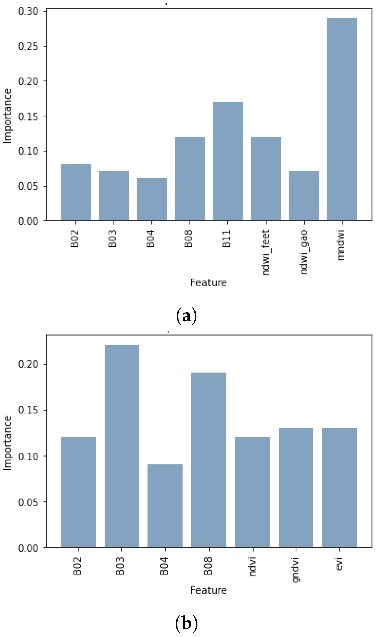
For the independent variables, based on the study results in the 2017–2018 campaigns, it was decided to generate different learning matrices, depending on the event to be found.

As far as the raw S2 data were concerned, the bands indicated in Table 2 were used for the flooding phase, and the same bands except for B11 were used for the vegetative development phase of the crop.

As far as level 3 S2 products were concerned, the NDWI indices by the McFeeters method, NDWI according to the Gao method [31], and the Modified Normalised Difference Water Index (MNDWI) [32] were used for the flooding stage.

$$NDWI=\frac{B8-B11}{B8+B11}$$

(3)

$$MNDWI=\frac{B3-B11}{B3+B11}$$

(4)

For the maximum vigour event, in addition to the S2 data, the NDVI index, the Green Normalised Difference Vegetation Index (GNDVI) [33], and the Enhanced Vegetation Index (EVI) [34] were used. These same features were also used for the cardinality check.

$$GNDVI=\frac{B8-B3}{B8+B3}$$

(5)

$$EVI=\frac{2.5\ast (B8-B4)}{(B8+6.0\ast B4-7.5\ast B2)+1.0}$$

(6)

Table 4. Characteristics of the learning matrix by phase.

Phase	S2 Bands	Indices
Flooding	B2, B3, B4, B8, B11	NDWIfeet, NDWIgao, MNDWI
Growth	B2, B3, B4, B8	NDVI, GNDVI, EVI

shows a summary of the characteristics of the learning matrix per phase:

On this occasion, the learning matrix was not divided between training and test, but K-Fold cross-validation was used for model fitting and validation [35], with k = 5.

Finally, for the scaling of the learning matrix, a series of pre-tests were conducted, comparing the results obtained with the scaled and unscaled matrix, and no representative improvements were observed.

4.2.5. Machine Learning Classification

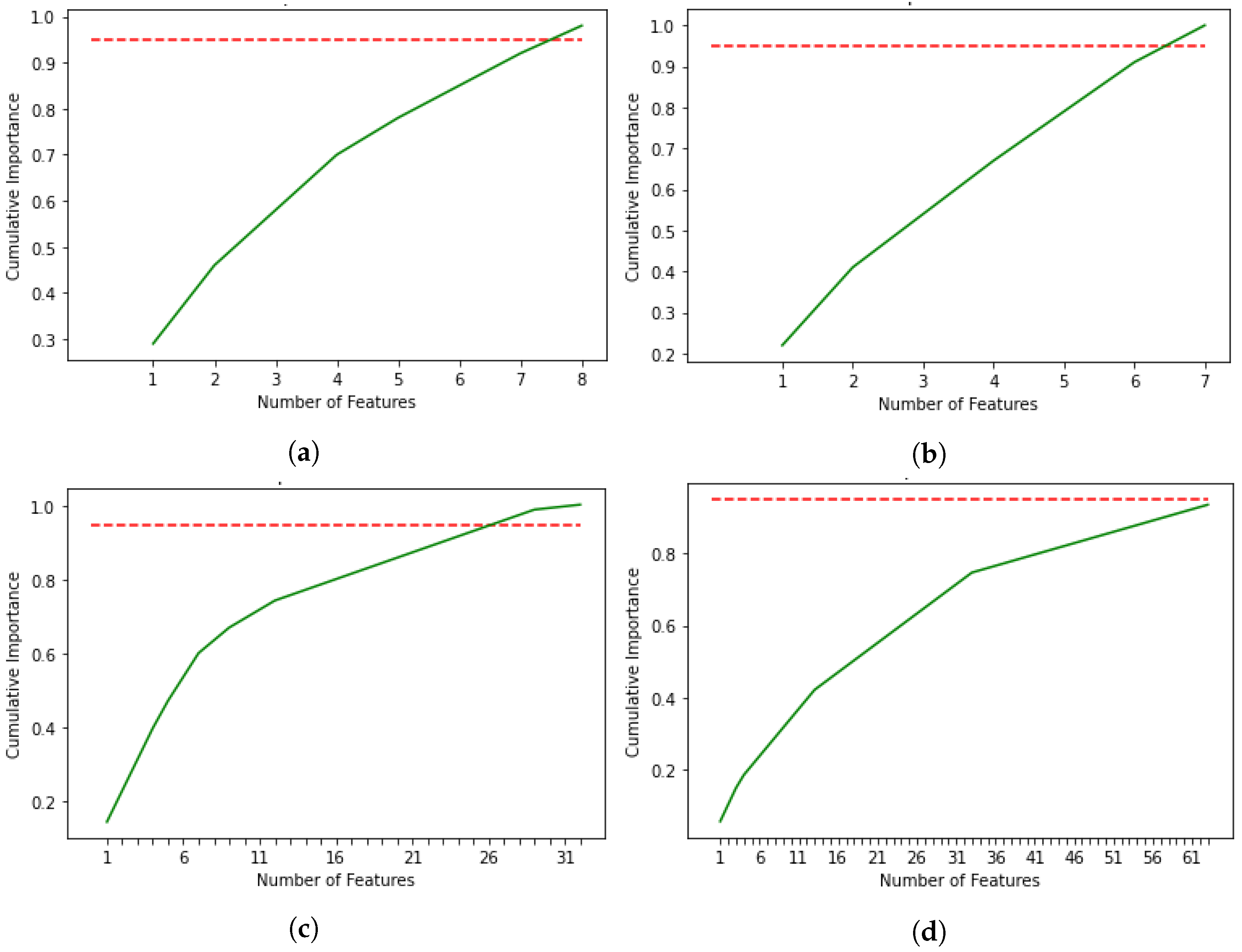
In the defined methodology, two classifications were generated with machine learning in raster format, both at a pixel level. The only difference between the two was the learning matrix.

The first one, called classification with machine learning at the moment (CLAML-M), only included in the learning matrix the features indicated in the previous section (Section 4.2.4), depending on the phenological phase of the crop, for the specific date on which the algorithm was executed.

The second one was called classification with machine learning with cumulative time series (CLAML-TS), and the learning matrix was composed of the same features as in the previous case but accumulating the features of the previously processed dates within the same phenological phase [36]. Thus, toward the end of the flooding phase, the learning matrix had the base characteristics corresponding to the dates: 20 May 2020, 30 May 2020, 14 June 2020, and 29 June 2020, which resulted in a raster with about 30 bands. These images generated a raster with about 30 bands. By the end of the phase of maximum crop development, the learning matrix was composed of the features corresponding to the dates, 4 July 2020, 9 July 2020, 19 July 2020, 23 July 2020, 29 July 2020, 8 August 2020, 18 August 2020 and 28 August 2020, obtaining approximately 60 bands.

Once the learning matrix was available, the RF classifier [37] was used as a model, optimising specific hyperparameters [38] through K-Fold cross-validation, with k = 5. The parameters evaluated in this optimisation process were the number of estimators, the function that measures the quality of the splits, the maximum number of features, the maximum depth, the minimum elements of a split, the minimum elements of a leaf, the maximum number of nodes per leaf, and the weights associated with the classes.

With our optimised and adjusted model, a validation of the model was carried out with the whole learning matrix through K-Fold cross-validation, with k = 5, and ending with the storage in a database of the mean values and the standard deviation of different metrics, such as accuracy, precision, F1 score, and recall.

With the RF classifier optimised and adjusted, the prediction was carried out on the total surface of the study area, and as a result, two different classifications were obtained, both at a pixel level. These classifications were translated into a raster composed of three bands, the first one relating to the prediction class, the second one with the probability that it was not rice, and the third one with the probability that it was rice.

In order to be able to issue a traffic light colour for each of the agricultural plots, as indicated in the CAP monitoring technical guidelines, it was necessary to move from a classification by pixel to a classification by the object at the enclosure level. For this purpose, the algorithm obtained different zonal statistics between the raster resulting from the RF classification and the parcel with the aid declarations. At this point, generic statistics were stored, such as the mean, standard deviation, number of pixels, or majority, and others were created on-demand, such as the number of rice class and non-rice class pixels, the average probability of the prediction for the rice class pixels and the non-rice class pixels.

On the zonal statistics of the previous paragraph, an adjustment was made, consisting of analysing the results obtained by excluding the pixels on the perimeter of the enclosure. Once these pixels were excluded, statistical information was generated regarding the number of pixels, the number of pixels in the rice class and non-rice class, and the average prediction probability for pixels classified as rice and for those classified as non-rice.

In short, this part of the methodology generated more than 80 parameters, which, to a greater or lesser extent, had a direct impact on the light traffic colour established on the enclosures.

4.2.6. Traditional Decision Tree

The final step in the defined methodology consisted of introducing all the information generated by analysing the biophysical indices and the RF classifications into a traditional decision tree. Depending on the crop phase in which we found ourselves, one data set prevailed over another.

Thus, in the flooding phase, the set of results that carried the most weight was CLAML-TS, followed by CLAML-M, and traditional remote sensing, with the NDWI flooding index, only came into play if the RF classifications raised doubts because the number of pixels labelled as rice was very close to the defined threshold (60%). On the other hand, for the crop development phase, the NDVI vegetation index had to be above the predefined threshold (0.54) obtained from the crop survey in the area in the 2017 and 2018 campaigns. In addition, the number of pixels marked as rice had to be above the parametrised threshold (60%) in the RF classifications.

The decision tree also continued the status of the traffic lights until the next phase. So, if it was established that a specific enclosure had been flooded, the green colour of the traffic light was automatically set for all subsequent dates until the crop growth phase was reached. The same was true for the vegetative growth phase of the crop. On the other hand, if an enclosure was established as non-flooded, it automatically turned red at the end of the flooding phase. It was considered that flooding of the agricultural plot was a prerequisite for it to be considered to be rice cultivated.

The so-called cardinality check was introduced, referring to whether 100% of the declared area was cultivated on an enclosure. This condition was analysed in the traditional decision tree toward the end of crop development, i.e., end of August or beginning of September. For this point to be considered, the enclosure had to arrive with the green traffic light, and only the results obtained by the RF classifications were taken into account. This point defined a very restrictive threshold on the number of pixels detected as rice without considering those included in the perimeter of the plot. To assume that a plot complied with the cardinality principle, 80% of the pixels, excluding the periphery, had to be labelled as the rice class.

5. Results

This section discusses in detail the metrics obtained by the RF models, an analysis of how the selected features influenced the RF-generated models, the results of the quality assessment that was performed based on the technical guidelines issued by the JRC, and a comparison of the results obtained by the different methods individually, without resorting to the traditional decision tree.

5.1. Machine Learning Metrics

The tool implemented, in this work, recorded a varied number of metrics each time the process was executed, both for CLAML-M and CLAML-TS.

Table 5. CLAML-M metrics values.

Date	Accuracy	Precision	Recall	F1	Kappa	AUC
20 May 2020	0.95	0.95	0.97	0.96	0.87	0.93
30 May 2020	0.97	0.98	0.98	0.98	0.94	0.97
14 June 2020	0.96	0.97	0.98	0.97	0.92	0.96
29 June 2020	0.93	0.94	0.96	0.95	0.82	0.91
4 July 2020	0.91	0.93	0.94	0.93	0.78	0.89
9 July 2020	0.91	0.92	0.95	0.93	0.78	0.88
19 July 2020	0.89	0.90	0.95	0.92	0.74	0.86
24 July 2020	0.90	0.91	0.95	0.93	0.76	0.87
29 July 2020	0.91	0.92	0.95	0.93	0.78	0.88
8 August 2020	0.92	0.92	0.96	0.94	0.80	0.89
13 August 2020	0.91	0.91	0.95	0.93	0.79	0.89
18 August 2020	0.90	0.91	0.94	0.92	0.79	0.89
28 August 2020	0.93	0.94	0.96	0.95	0.85	0.92

and

Table 6. CLAML-TS metrics values.

Date	Elements	Accuracy	Precision	Recall	F1	Kappa	AUC
20 May 2020	1	0.95	0.95	0.98	0.96	0.87	0.93
30 May 2020	2	0.98	0.99	0.98	0.99	0.96	0.98
14 June 2020	3	0.99	0.99	0.99	0.99	0.97	0.99
29 June 2020	4	0.99	0.99	0.99	0.99	0.97	0.98
04 July 2020	1	0.91	0.93	0.94	0.93	0.78	0.89
9 July 2020	2	0.94	0.95	0.97	0.96	0.86	0.93
19 July 2020	3	0.97	0.98	0.98	0.98	0.94	0.97
24 July 2020	4	0.97	0.98	0.98	0.98	0.94	0.97
29 July 2020	5	0.98	0.98	0.98	0.98	0.95	0.97
8 August 2020	6	0.98	0.98	0.98	0.98	0.95	0.97
13 August 2020	7	0.98	0.98	0.98	0.98	0.95	0.98
18 August 2020	8	0.98	0.98	0.98	0.98	0.95	0.98
28 July 2020	9	0.98	0.98	0.99	0.99	0.96	0.98

show the values, for each of the runs, of the metrics recorded by the two types of ML classification implemented (Section 4.2.5).

From the above tables, we obtain the mean values and the standard deviation reflected in the corresponding

Table 7. Mean values and standard deviation of metrics.

Product	Accuracy	Precision	Recall	F1	Kappa	AUC
CLAML-M	0.92 (0.02)	0.93 (0.02)	0.96 (0.01)	0.94 (0.02)	0.81 (0.06)	0.90 (0.03)
CLAML-TS	0.97 (0.02)	0.98 (0.02)	0.98 (0.01)	0.98 (0.02)	0.93 (0.06)	0.96 (0.03)

.

Graphically, Figure 5 shows the evolution of some metrics of the two RF classifiers implemented with successive runs.

In summary, it can be observed that the CLAML-TS metric scores were systematically better than CLAML-M metrics as dates were added to the time series.

5.2. Features Importance

Thanks to the metrics generated by the algorithm implemented in this work, it was possible to analyse the use made by the models of the features provided in the learning matrix.

Figure 6 shows that, to some extent, no single characteristic becomes more prominent than the others.

Another way to analyse this information is to generate the cumulative importance that shows the contribution to the overall importance of each additional variable, which can be seen in Figure 7. The dashed line is set at 95% of the total accounted importance, which, although an arbitrary threshold, can be the meeting point between the model performance and optimisation.

It can be seen from the figure above that the features that made a residual contribution to the model performance were unrepresentative. Even in the CLAML-TS model for the flooding phase, all features in the learning matrix were of considerable importance.

5.3. Quality Evaluation

Following the end of the 2020 agricultural season, a quality assessment of the monitoring was carried out, following the guidelines issued by the Joint Research Centre (JRC) [39]. This quality assessment was based on the international standard ISO 2859/2 [40] and had associated acceptance numbers that indicated whether or not the tests were passed depending on the errors found. In addition, a series of batches were created to define the events or milestones to be evaluated.

In this quality assessment, the implemented algorithm’s performance was tested to identify the rice crop and the so-called cardinality. Each batch was assigned a sample of 200 elements, which did not have to coincide with each other. Supporting material included the S2 images used for automatic monitoring and a high-resolution image of the study area from the Pleiades-1 satellite, with a spatial resolution of 50cm, taken at the beginning of September.

The results found zero errors for the crop identification batch and two for the cardinality batch. With the errors obtained, the tests were considered to have passed.

For example, in Figure 8, what looks like an area of trees and even a small building was included in the aid declaration in the lower right part of the figure. The model marks this area as non-rice (red), correctly. The threshold corresponding to the cardinality, which corresponds to the minimum percentage of pixels labelled with the rice class (green), should be increased to avoid error.

5.4. Biophysical Indices vs. CLAML-M vs. CLAML-TS

Thanks to the information gathered during the quality assessment process, we were able to compare the results that would have been obtained, in the hypothetical case of not implementing the traditional decision tree, to the joint treatment of the results obtained by the intermediate products, i.e., biophysical indices and the classifications by RF CLAML-M and CLAML-TS.

For the rice crop identification batch, we found the error ratio reflected in

Table 8. Errors in batch of crop identification with individual treatment.

Product	Errors	False Positives	False Negatives
Biophysical Indices	16	9	7
CLAML-M	4	2	2
CLAML-TS	2	0	2

.

For the batch associated with cardinality,

Table 9. Errors in cardinality batch with individualised treatment.

Product	Errors	False Positives	False Negatives
CLAML-M	32	32	0
CLAML-TS	2	2	0

lists the errors that would have been obtained if the intermediate products were treated individually. In this batch, the results related to the biophysical indices were not treated, as it is not possible to check cardinality with this type of product.

For the crop identification batch, combining the data generated by the three intermediates gave optimal results. This situation is more evident in the case of the cardinality batch.

Analysing the detailed data from which Table 8 and Section 5.3 are derived, it was observed that, in the case of the crop identification batch, the combination of the three products generated within the decision tree succeeded in eliminating the errors of the CLAML-TS product. In contrast, the errors of the CLAML-TS product for the cardinality batch (Table 9) were not corrected by introducing the CLAML-M product into the final decision tree.

6. Conclusions

Crop monitoring controls based on satellite imagery aim to perform a periodic and continuous check that verifies the activity declared by the farmer, observed through time series of images. In this work, we proposed a decision support system based on ML, S2 imagery, and derived products that allow the simple integration of heterogeneous data sources to assist and improve the decision-making process on granting CAP subsidies. The foreseeable savings in field trips and in situ controls will improve the efficiency in the management and granting of aid promoted by the CAP.

The methodology defined is based on combining the crop phenology being identified, in this case, rice, with S2 images and the land parcel with the aid applications. As the process must be carried out continuously throughout the campaign, and depending on the agricultural practices applied for each phenological phase of the crop, the characteristics used were rotated in such a way as always to use those that helped to determine the crop in question uniquely. In parallel, data were generated from three different sources: biophysical indices, RF classification on a pixel-by-pixel basis for a specific point in time, and RF classification using a cumulative time series at a pixel level. Since any improvement, however small, directly impacted better management and distribution of CAP resources, it was decided to implement a traditional decision tree to which the data obtained from the three previous sources were introduced. Finally, a chromatic indicator was issued to indicate whether the requested aid obligations were being met (green) or not (red) or whether the automatic system could not issue a verdict (yellow).

The algorithm associated with the methodology was run 13 times, one for each available zero cloud cover image of the study area, resulting in RF classifications with an accuracy of 92% (+/− 0.02%) at the moment (CLAML-M) and 97% (+/− 0.02%) in the time series (CLAML-TS), while traditional biophysical indices reported a 16% error. At this point, it was clear that RF classification using cumulative time series gave the best results. With the introduction of the final decision tree, which evaluated the results of each of these three products with different weights, the quality control was 100 percent effective in terms of pure rice crop identification and 99 percent effective in terms of cardinality.

An improvement of this line of research would be to introduce the concept of feature engineering by incorporating into the learning matrix information related to the location (using the coordinates of each pixel or location within a matrix using row and column), and detailed date information, such as the number of the day, month, year, number of the day of the week, or number of the week within the year. Moreover, it is considered necessary to carry out a study on how dimensionality reduction or feature selection affects the final performance of the model. In addition, this methodology can be extrapolated to identify other types of crops in a larger study area. Finally, we intend to use deep learning to identify the rice crop and to compare the results obtained with the results of this work. Another would be to define the neural network that would use the learning matrix of this work to make predictions. One other possibility would be related to artificial vision applied to satellite images employing convolutional neural networks [41] thanks to semantic segmentation architectures [42,43].

References

1. Erklavec, U.; Birt, C.; Pushkarev, N. Common Agricultural Policy (CAP) from a Public Health Perspective. Eur. J. Public Health 2021, 31, ckab164-188. [Google Scholar] [CrossRef]
2. Lozano-Tello, A.; Fernández-Sellers, M.; Quirós, E.; Fragoso-Campón, L.; García-Martín, A.; Gutierrez Gallego, J.A.; Mateos, C.; Trenado, R.; Muñoz, P. Crop identification by massive processing of multiannual satellite imagery for EU common agriculture policy subsidy control. Eur. J. Remote Sens. 2021, 54, 1–12. [Google Scholar] [CrossRef]
3. Jutz, S.; Milagro-Pérez, M. Copernicus: The European Earth Observation Programme. Rev. Teledetección 2020, 56. [Google Scholar] [CrossRef]
4. Pallathadka, H.; Mustafa, M.; Sanchez, D.T.; Sajja, G.S.; Gour, S.; Naved, M. Impact of machine learning on management, healthcare and agriculture. Mater. Today Proc. 2021; in press. [Google Scholar]
5. Maimaitijiang, M.; Sagan, V.; Sidike, P.; Daloye, A.M.; Erkbol, H.; Fritschi, F.B. Crop Monitoring Using Satellite/UAV Data Fusion and Machine Learning. Remote Sens. 2020, 12, 1357. [Google Scholar] [CrossRef]
6. Schulz, C.; Holtgrave, A.K.; Kleinschmit, B. Large-scale winter catch crop monitoring with Sentinel-2 time series and machine learning–An alternative to on-site controls? Comput. Electron. Agric. 2021, 186, 106173. [Google Scholar] [CrossRef]
7. Segarra, J.; Buchaillot, M.L.; Araus, J.L.; Kefauver, S.C. Remote sensing for precision agriculture: Sentinel-2 improved features and applications. Agronomy 2020, 10, 641. [Google Scholar] [CrossRef]
8. Tong, X.; Brandt, M.; Hiernaux, P.; Herrmann, S.; Rasmussen, L.V.; Rasmussen, K.; Tian, F.; Tagesson, T.; Zhang, W.; Fensholt, R. The forgotten land use class: Mapping of fallow fields across the Sahel using Sentinel-2. Remote Sens. Environ. 2020, 239, 111598. [Google Scholar] [CrossRef]
9. Sharifi, A. Using sentinel-2 data to predict nitrogen uptake in maize crop. IEEE J. Sel. Top. Appl. Earth Obs. Remote Sens. 2020, 13, 2656–2662. [Google Scholar] [CrossRef]
10. López-Andreu, F.J.; Erena, M.; Dominguez-Gómez, J.A.; López-Morales, J.A. Sentinel-2 Images and Machine Learning as Tool for Monitoring of the Common Agricultural Policy: Calasparra Rice as a Case Study. Agronomy 2021, 11, 621. [Google Scholar] [CrossRef]
11. NaLamKI Project. Available online: https://nalamki.de/ (accessed on 3 November 2021).
12. knowlEdge Project. Available online: https://www.knowledge-project.eu/ (accessed on 15 November 2021).
13. Facchinetti, D.; Santoro, S.; Galli, L.E.; Fontana, G.; Fedeli, L.; Parisi, S.; Bonacchi, L.B.; Šušnjar, S.; Salvai, F.; Coppola, G.; et al. Reduction of Pesticide Use in Fresh-Cut Salad Production through Artificial Intelligence. Appl. Sci. 2021, 11, 1992. [Google Scholar] [CrossRef]
14. Serale, G.; Gnoli, L.; Giraudo, E.; Fabrizio, E. A Supervisory Control Strategy for Improving Energy Efficiency of Artificial Lighting Systems in Greenhouses. Energies 2021, 14, 202. [Google Scholar] [CrossRef]
15. Sarvia, F.; Xausa, E.; Petris, S.D.; Cantamessa, G.; Borgogno-Mondino, E. A Possible Role of Copernicus Sentinel-2 Data to Support Common Agricultural Policy Controls in Agriculture. Agronomy 2021, 11, 110. [Google Scholar] [CrossRef]
16. Siesto, G.; Fernández-Sellers, M.; Lozano-Tello, A. Crop Classification of Satellite Imagery Using Synthetic Multitemporal and Multispectral Images in Convolutional Neural Networks. Remote Sens. 2021, 13, 3378. [Google Scholar] [CrossRef]
17. Portalés-Julià, E.; Campos-Taberner, M.; García-Haro, F.J.; Gilabert, M.A. Assessing the Sentinel-2 Capabilities to Identify Abandoned Crops Using Deep Learning. Agronomy 2021, 11, 654. [Google Scholar] [CrossRef]
18. Ramadhani, F.; Pullanagari, R.; Kereszturi, G.; Procter, J. Automatic mapping of rice growth stages using the integration of SENTINEL-2, MOD13Q1, and SENTINEL-1. Remote Sens. 2020, 12, 3613. [Google Scholar] [CrossRef]
19. Chang, L.; Chen, Y.T.; Wang, J.H.; Chang, Y.L. Rice-Field Mapping with Sentinel-1A SAR Time-Series Data. Remote Sens. 2021, 13, 103. [Google Scholar] [CrossRef]
20. Nazir, A.; Ullah, S.; Saqib, Z.A.; Abbas, A.; Ali, A.; Iqbal, M.S.; Hussain, K.; Shakir, M.; Shah, M.; Butt, M.U. Estimation and Forecasting of Rice Yield Using Phenology-Based Algorithm and Linear Regression Model on Sentinel-II Satellite Data. Agriculture 2021, 11, 1026. [Google Scholar] [CrossRef]
21. Sitokonstantinou, V.; Koukos, A.; Drivas, T.; Kontoes, C.; Papoutsis, I.; Karathanassi, V. A Scalable Machine Learning Pipeline for Paddy Rice Classification Using Multi-Temporal Sentinel Data. Remote Sens. 2021, 13, 1769. [Google Scholar] [CrossRef]
22. Regulatory Council Calasparra Designation of Origin. Available online: https://docalasparra.com (accessed on 26 November 2021).
23. Copernicus Open Access Hub API. Available online: https://scihub.copernicus.eu/twiki/do/view/SciHubWebPortal/APIHubDescription (accessed on 25 November 2021).
24. Fukai, S. Phenology in rainfed lowland rice. Field Crop. Res. 1999, 64, 51–60. [Google Scholar] [CrossRef]
25. European Space Agency. Available online: https://www.esa.int (accessed on 25 November 2021).
26. Berger, M.; Moreno, J.; Johannessen, J.A.; Levelt, P.F.; Hanssen, R.F. ESA’s sentinel missions in support of Earth system science. Remote Sens. Environ. 2012, 120, 84–90. [Google Scholar] [CrossRef]
27. e Santos, D.A.; Martinez, J.; Harmel, T.; Borges, H.; Roig, H. Evaluation Of Sentinel-2/Msi Imagery Products Level-2a Obtained By Three Different Atmospheric Corrections For Monitoring Suspended Sediments Concentration In Madeira River, Brazil. In Proceedings of the 2020 IEEE Latin American GRSS & ISPRS Remote Sensing Conference (LAGIRS), Santiago, Chile, 22–26 March 2020; pp. 207–212. [Google Scholar]
28. Stromann, O.; Nascetti, A.; Yousif, O.; Ban, Y. Dimensionality reduction and feature selection for object-based land cover classification based on Sentinel-1 and Sentinel-2 time series using Google Earth Engine. Remote Sens. 2020, 12, 76. [Google Scholar] [CrossRef] [Green Version]
29. Tucker, C. Red and Photographic Infrared Linear Combinations for Monitoring Vegetation. Remote Sens. Environ. 1979, 8, 127–150. [Google Scholar] [CrossRef] [Green Version]
30. McFeeters, S.K. The use of the Normalized Difference Water Index (NDWI) in the delineation of open water features. Int. J. Remote Sens. 1996, 17, 1425–1432. [Google Scholar] [CrossRef]
31. Gao, B.C. NDWI—A normalized difference water index for remote sensing of vegetation liquid water from space. Remote Sens. Environ. 1996, 58, 257–266. [Google Scholar] [CrossRef]
32. Xu, H. Modification of normalised difference water index (NDWI) to enhance open water features in remotely sensed imagery. Int. J. Remote Sens. 2006, 27, 3025–3033. [Google Scholar] [CrossRef]
33. Gitelson, A.A.; Kaufman, Y.J.; Merzlyak, M.N. Use of a green channel in remote sensing of global vegetation from EOS-MODIS. Remote Sens. Environ. 1996, 58, 289–298. [Google Scholar] [CrossRef]
34. Huete, A.; Didan, K.; Miura, T.; Rodriguez, E.P.; Gao, X.; Ferreira, L.G. Overview of the radiometric and biophysical performance of the MODIS vegetation indices. Remote Sens. Environ. 2002, 83, 195–213. [Google Scholar] [CrossRef]
35. A Ramezan, C.; A Warner, T.; E Maxwell, A. Evaluation of sampling and cross-validation tuning strategies for regional-scale machine learning classification. Remote Sens. 2019, 11, 185. [Google Scholar] [CrossRef] [Green Version]
36. Sitokonstantinou, V.; Papoutsis, I.; Kontoes, C.; Lafarga Arnal, A.; Armesto Andrés, A.P.; Garraza Zurbano, J.A. Scalable parcel-based crop identification scheme using Sentinel-2 data time-series for the monitoring of the common agricultural policy. Remote Sens. 2018, 10, 911. [Google Scholar] [CrossRef] [Green Version]
37. Thanh Noi, P.; Kappas, M. Comparison of random forest, k-nearest neighbor, and support vector machine classifiers for land cover classification using Sentinel-2 imagery. Sensors 2018, 18, 18. [Google Scholar] [CrossRef] [Green Version]
38. Lujan-Moreno, G.A.; Howard, P.R.; Rojas, O.G.; Montgomery, D.C. Design of experiments and response surface methodology to tune machine learning hyperparameters, with a random forest case-study. Expert Syst. Appl. 2018, 109, 195–205. [Google Scholar] [CrossRef]
39. Joint Research Centre (JRC). Available online: https://ec.europa.eu/jrc/en (accessed on 25 November 2021).
40. ISO 2859-2. Available online: https://www.iso.org/obp/ui/#iso:std:iso:2859:-2:ed-1:v1:en (accessed on 26 November 2021).
41. Hsieh, T.H.; Kiang, J.F. Comparison of CNN algorithms on hyperspectral image classification in agricultural lands. Sensors 2020, 20, 1734. [Google Scholar] [CrossRef] [PubMed] [Green Version]
42. Wei, S.; Zhang, H.; Wang, C.; Wang, Y.; Xu, L. Multi-temporal SAR data large-scale crop mapping based on U-Net model. Remote Sens. 2019, 11, 68. [Google Scholar] [CrossRef] [Green Version]
43. Zhang, M.; Jing, W.; Lin, J.; Fang, N.; Wei, W.; Woźniak, M.; Damaševičius, R. NAS-HRIS: Automatic design and architecture search of neural network for semantic segmentation in remote sensing images. Sensors 2020, 20, 5292. [Google Scholar] [CrossRef] [PubMed]
Figure 1. Plots located in Coto Arrocero, Calasparra (Murcia).
Electronics 11 00325 g001
Figure 2. Most representative stages of rice cultivation in the study area. (a) Flooded plot. (b) Plot in growth phase.
Electronics 11 00325 g002
Figure 3. Scheme representing the methodology followed to identify and monitor different crops.
Electronics 11 00325 g003
Figure 4. NDVI and NDWI indices of S2 for the study area. (a) NDWI index dated 30 May 2020 in the study area. (b) NDVI index dated 28 August 2020 in the study area.
Electronics 11 00325 g004
Figure 5. Metrics scoring. (a) Accuracy metric scoring. (b) Kappa metric scoring.
Electronics 11 00325 g005
Figure 6. Feature importance. (a) Feature importance in CLAML-M model for flooding. (b) Feature importance in CLAML-M model for growth.
Electronics 11 00325 g006
Figure 7. Cumulative importance. (a) Cumulative importance CLAML-M NDWI. (b) Cumulative importance CLAML-M NDVI. (c) Cumulative importance CLAML-TS NDWI. (d) Cumulative importance CLAML-TS NDVI.
Electronics 11 00325 g007
Figure 8. Example of error detected in the quality assessment on the cardinality batch. (a) Orthophoto on the enclosure with the wrong traffic light colour in cardinality. (b) Classification by RF on the enclosure with the wrong traffic light colour in cardinality.
Electronics 11 00325 g008