Performance Analysis of Multi-User MIMO Schemes under Realistic 3GPP 3-D Channel Model for 5G mmWave Cellular Networks

Abstract

Novel techniques such as mmWave transmission and massive MIMO have proven to present many attractive features able to support high data demand for 5G NR technologies. Towards the standardization of 5G networks, channel modeling has become an important step in order to test the reliability of theoretical studies. In this paper, we study the performance of a 5G network at mmWave range for the downlink. We consider a single trisectorized base station equipped with planar arrays, and we model users as a spatial Poisson process in a hexagonal grid. We adopt the latest 3GPP channel model described in TR 38.901 and we provide a thorough description and step-by-step tutorial of it along with our customizations and MATLAB scripts for channel generation in the presented scenario. Moreover, we evaluate the performance of Multi-User Multi-Layer MIMO techniques, such as Signal-to-Leakage-plus-Noise Ratio (SLNR) precoding and MMSE combined with different system configurations by means of achievable per-user rate.

1. Introduction

Over the last decades, mobile communications have caught a lot of interest in our everyday life. During the 1980s, the first standard of mobile communications was launched and our lives changed dramatically in many aspects. Studies such as [1,2] show how the use of mobile devices has changed our behavior in the social sphere. Before the advent of wireless communications, we were not able to do things that we now label as everyday activities, such as call the office while driving our car or having multiple video-calls with our friends scattered over the world. The digitization process started in the early 1990s with the roll-out of the second generation of mobile communication devices (2G). The continuous deployment of new services, with the increase in data demand [3], has led to the novel fifth generation standard (5G) for wireless communications.

During the past years, research about mobile communications has been moving quickly through the different standards of communications, but there is still a certain distance between theoretical studies and practical applications. The validation of analytical models became a crucial step in the standardization process. Ideally, it is preferable to test everything through physical, real time prototypes, but this is possible only after standardization due to the high cost of development. Usually, many trials may be conducted in the field to help the research stage of the technology, although they bring a limited contribution. Field trials can be combined with numerical simulations to validate the studies during the research stage of the standardization. Therefore, in order to obtain significant numerical results for a communication system, a strong channel model is required to regard the behavior of the signals through the physical space between transmitters and receivers, attenuations through the paths, atmospheric conditions, etc.

The millimeter wave (mmWave) frequency spectrum presents many attractive features able to support high data demand for 5G NR technologies such as good propagation behavior in line-of-sight (LOS) scenarios. Available bandwidths in that range of frequencies under 5G regulatory consideration, i.e., from 27 to 71 GHz, are much wider than all currently adopted cellular allocations [4,5,6]. The reduced wavelengths will pave the way for the implementation of massive multiple-input and multiple-output (MIMO) techniques such as precoding or beamforming. However, mmWave communications bring new challenges for the research community in order to develop a unified channel model, as this range of frequencies is more vulnerable to path attenuation, noise, interference, and atmospheric attenuation due to adverse weather conditions and other environmental effects. Channel models used for 4G communications make the assumption of 2-D propagating waves, which is plausible due to the fact that the angular spectrum is negligible. In mmWave communications, this assumption is no longer valid, so that a good channel model for 5G has to overtake the assumption of propagation only on the horizontal plane, and it needs to foresee a 3-D channel model [7].

Several new technologies have been proposed for 5G cellular networks, such as Massive MIMO, Non-orthogonal multiple access (NOMA) [8], and cognitive radios [9,10] by means of spectrum sensing [11,12,13,14] to support operations in unlicensed spectrum. In particular, Space Division Multiple Access (SDMA) or Multi-User MIMO techniques are one of the most promising features to improve the operation of 5G networks, essential to deal with the growing demand of data rates, caused by new services such as Ultra-High Definition (UHD) video, virtual reality (VR), and augmented reality (AR). Antenna arrays with a large number of antenna elements will facilitate both the path loss compensation and the management of the inter-user interference, by taking advantage of sophisticated precoding solutions such as the Signal-to-Leakage-plus-Noise ratio (SLNR), Zero-Forcing (ZF) [15], or Minimum Mean Square Error (MMSE) [16] precoding schemes. In particular, SLNR precoding [17] addresses the minimization of the interference caused by a user device (leakage) to all other devices in the corresponding frequency or time resource, while maximizing the received desired signal power for every user. A generation of SLNR precoding to MIMO orthogonal frequency division multiplexing (OFDM) multi-user systems is studied in [18]. In [19], the authors prove the equivalence between MMSE and SLNR precoding schemes under equal power allocation (EPA). In [20] an enhanced SLNR precoding, called layer SLNR, deals with the case of multiple data streams for each user, by minimizing the inter-layer interference both from the same user and from different users.

The application of MU-MIMO techniques to realistic 3-D channel models is somewhat limited in the literature. In this paper, we focus on a Multi-User Multi-Layer downlink communication scheme: we adopt a SLNR precoder at the transmitter with an approach similar to [20], and we implement a MMSE receiver or combiner at each receiver. The adopted communication channel is the 5G-compliant 3GPP spatial channel model described in the Technical Report 38.901 entitled “Study on channel model for frequency spectrum above 6 GHz” [21].

1.1. State of the Art for Channel Modeling

The literature presents many channel models, and generally two main approaches are taken into account: stochastic and statistical. The first is based on a step-by-step analysis of the probability density function (PDF) of the channel parameters which are based on the geometry of the considered scenario. Stochastic models are easy and quick to formulate, but they cannot be completely validated without field measurements data or through a ray-tracing analysis. Meanwhile, statistical models can be formulated after exhaustive measurements on the field and a successive formulation based on the data. The model obtained through this approach is limited for the region of the measurements, and the final data can suffer from a significant variation depending on the geographical location. Moreover, a statistical model can suffer from low accuracy related to the used instruments and the post-processing method.

To overcome the drawbacks of these strategies, a hybrid approach is the most widely adopted, in which the channel parameters can be stochastically characterized by studying their probability distributions. Then, field measurements can be adopted to verify the first step and eventually modify the channel model [22]. Regardless of the adopted strategy, MIMO channel models for mmWave system level simulations mainly use the Clustered Delay Line (CDL) model in which the scatterers are grouped into clusters distributed over the area. Each cluster contains multipath elements with the same delay and small variations in angles of departure and arrival.

A milestone for the channel modeling has been provided by the Information Society Technologies (IST) with the Wireless World Initiative New Radio (WINNER) project. In 2007, they released the deliverable WINNER II [23], as an evolution of the WINNER I project, providing channel models for link level and system level simulations in many scenarios such as local area, metropolitan area, and wide area. They offered a 2-D stochastic channel model approach which is geometry-based and antenna independent (i.e., different antenna configurations and element patterns can be used). They provide a hybrid approach, and the channel instances are generated by combining the outcomes of rays with particular channel parameters (power, delay, and angle of arrival and departure). WINNER II offers the capability to cover scenarios with both indoor and outdoor users, elevation in indoor applications, and LOS and non-line-of-sight (NLOS) conditions, and the models are scalable from a SISO system to a MIMO system. The proposed channel modeling approach can be applicable to any wireless system operation in the 2–6 GHz frequency range with a variable bandwidth up to 100 MHz. In 2014, researchers presented the Quasi Deterministic Radio Channel Generator (QuaDRiGa) [24] project as an extension for the WINNER+ (the 3-D version of the WINNER II) [25] work. They presented a 3-D stochastic channel modeling approach introducing the time evolution [26,27] of the channel, which is fully available as MATLAB code [28]. The QuaDRiGa model is divided into two steps; in the first one, they offer a stochastic generation of the large scale parameters (LSPs) and the random 3-D positioning of the scattering clusters. They consider base stations with a fixed position while the user terminals can move, so that the scattering clusters are fixed and the channel is deterministic in its time evolution. The second phase is the validation of the model by measurements in downtown Berlin (Germany) by extracting single-link and multi-link parameters and observing that there is a good match between simulated and measured results. In its last version, QuaDRiga can support carrier frequencies in the range 0.45–100 GHz.

An example of geometry-based stochastic channel model (GBSM) is the mmMAGIC channel model [29], which is based on QuaDRiGa. Several measurements have been conducted in the main scenarios in the range between 6 GHz and 100 GHz. The model foresees frequency dependent large scale parameters and the number of cluster and rays generated as random variables instead of fixed numbers. Moreover, mmMAGIC supports bandwidths up to 2 GHz and is supposed to meet most of the 5G channel model requirements, however it is a high computational model that makes numerical simulations inefficient.

The METIS channel model [30] is able to achieve a more flexible and scalable methodology by providing a map-based model, a stochastic model and their combination: the hybrid model. The map-based model supports frequency ranges up to 70 GHz and uses a simplified 3-D geometric description of a propagation environment and additional randomly generated shadowing objects. The stochastic model (up to 100 GHz) is a GBSM legacy of WINNER strategy. Moreover, METIS proposes a simplified approach to generate spatially consistent LSPs through a sum of sinusoids [31,32], which results in a lower computational consumption, especially useful for D2D/V2V applications.

In [33] we can find the recent MG5GCM model as a combination of new advanced channel modeling techniques such as array-time evolution, spherical wavefront, etc. This model can meet many 5G channel requirements with a relatively low complexity, although it only takes small-scale fading into account and neglects large-scale fading. Furthermore, parameters for the model for different scenarios need to be extracted from future measurements. A different approach has been introduced in [34], where authors provide a machine learning based framework. In particular, they provide a time-varying channel modeling method by using a neural network to model and predict the path loss together with shadowing, fading and joint small scale parameters. Results from the neural network have been compared with measurements at 26 GHz performed in a microcell. A comprehensive 3GPP-like mmWave channel model called statistical spatial channel model (SSCM) has been proposed in [35,36,37] based on measurements in the range 28–73 GHz [38]. Differently from the 3GPP–WINNER strategies, they introduce the concepts of time clusters and spatial lobes, which can describe the temporal and spatial statistics independently.

1.2. Paper Contribution

The aim of this work is firstly to analyze the latest 3-D channel model for 5G (described in [21]) by 3GPP, in order to provide a tutorial of its implementation in MATLAB. Then we proceed to study the aforementioned channel model in a particularly interesting scenario, namely a trisectorial cell site with 5G-compliant communication parameters. We assume an Orthogonal Frequency-Division Multiplexing (OFDM) modulation and planar antenna arrays at the Base Station (BS) and User Terminals (UTs).

We resort to spatial multiplexing capabilities only to assess the system performance: UTs in the sector coverage area are served on the same time and frequency resources, by means of Space Division Multiple Access.

We finally simulate our system with different parameters (such as the antenna array size, the traffic loading, the total transmit power, etc.) in order to evaluate the link quality and the capacity with this new 3-D channel model. One of the target is to investigate the impact of different MIMO configurations on the per-user rate. Our main contributions are:

• Provide a step by step tutorial on the 3GPP Technical Report (TR) 38.901 channel model implementation along with MATLAB scripts to generate channel coefficients [39].
• Design an OFDM MIMO system with uniform planar arrays and dual polarized antenna elements with realistic radiation patterns.
• Implement SLNR precoding and MMSE combining to exploit Multi-User Multi-Layer MIMO and provide simulation results on the system behavior.

2. Scenario Description

In the TR 38.901 [21], 3GPP released its 3-D stochastic channel model for 5G mmWave massive MIMO communications in the range 0.5–100 GHz. A detailed procedure is provided to generate link level channel models. The model is applicable to a wide range of carrier frequencies, with particular attention to the mmWave range by taking care of weak propagation aspects such as atmosphere attenuation, and it supports large channel bandwidth (up to $10\%$ of the carrier frequency). One purpose of this work is to present a simplified version (i.e., single cell network, time-invariant channel) of the system level channel model proposed in 3GPP TR 38.901 developed in MATLAB. 3GPP adopts different scenario settings, such as Urban Micro street canyon (UMi), Urban Macro (UMa), Indoor-Office, Rural Macro (RMa), and Indoor Factory (InF); for each scenario, a complete set of parameters is provided, such as intersite distance, path loss computation, large and small scale parameters, etc. In our work, we focus on a simplified single-cell UMi scenario. However, please note the provided MATLAB scripts [39] can also generate channel coefficients for a simplified single-cell UMa scenario. with a trisectorized single cell and static users, i.e., a time-invariant channel model. The spatial channel model could be described as a MIMO cluster delay line, i.e., each coefficient is the superposition of different clusters of rays. Each angular cluster has its own parameters, such as delay, power, azimuth angle spread of arrival/departure, zenith angle spread of arrival/departure, etc.

2.1. Network Layout

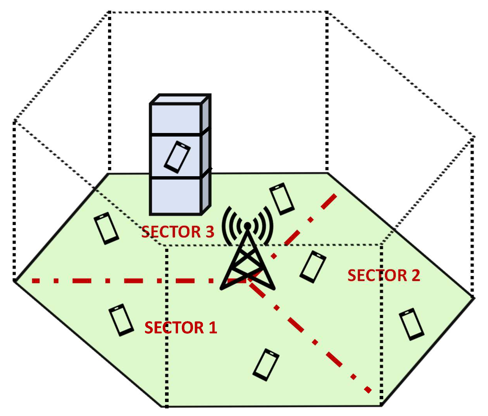
The scenario we adopted in this study is a typical hexagonal cell site divided in three sectors, each one covering a portion of 120 degrees in azimuth. Each sector is equipped with an antenna array, and the antenna parameters are the same for each sector. Figure 1 shows a representation of the cell site. The BS is placed at the center of the cell, represented as a hexagon of side or equivalently circumradius $R=100$ m, and with height $h_{BS}=10$ m.

The bounded area $\mathcal{A}$ of the hexagon can be computed as $\mathcal{A}=\frac{3\sqrt{3}}{2}{R}^2$. The random placement of the users inside $\mathcal{A}$ can be modelled as a spatial homogeneous Poisson point process. Denoting as $M\left(\mathcal{A}\right)$ the random variable corresponding to the amount of users of a point process present in the area $\mathcal{A}\subset {\mathbb{R}}^2$, the probability of K users existing in $\mathcal{A}$ can be expressed as:

$$\mathrm{Pr}[M\left(\mathcal{A}\right)=K]=\frac{{\left(\mu \mathcal{A}\right)}^K}{K!}{e}^{-\mu \mathcal{A}}$$

(1)

where $\mu$ (users/km²) is the average user density per unit area. A homogeneous process implies constant $\mu$, moreover $\mu$ does not depend on the location. Given K users of the Poisson process in $\mathcal{A}$, they are conditionally independent and uniformly distributed in the hexagon. Therefore, the positions of the randomly deployed K users can be determined by generating both the x and y coordinates. We denote with X, the abscissa of a generic user in the hexagon, where X is the marginal random variable of a uniform 2-D distribution in the cell site. In order to find it, let us first define the two random variables $X_1$ and $X_2$:

$$X_1\sim \mathcal{U}\left(-\frac{3}{4}R,\frac{3}{4}R\right)$$

(2)

$$X_2\sim \mathcal{U}\left(-\frac{1}{4}R,\frac{1}{4}R\right)$$

(3)

then we have:

$$X=X_1+X_2$$

(4)

where X is the sum of two uniform random variables with different bounds, the probability density function (pdf) of X is the convolution of the two uniform pdfs, resulting in a trapezoidal distribution. Once the abscissa is found, the conditional distribution of $Y|X=x$, where Y is the ordinate of the user, is given by:

$$\left\{\begin{array}{cc}\mathcal{U}\left(-\frac{\sqrt{3}}{2}R,\frac{\sqrt{3}}{2}R\right)\hfill & \left|x\right|\le R/2\hfill \\ \mathcal{U}\left(-\sqrt{3}(R-|x\left|\right),\sqrt{3}(R-|x|\right)\hfill & \left|x\right|>R/2\hfill \end{array}\right.$$

(5)

As we are developing a 3-D channel model, the height of the UTs must be determined subsequently. For outdoor users, the height is fixed at $1.5$ m. For indoor users, first of all we need to generate the number of floors of the building in which the user is placed. According to the TR 38.873 [40], we can generate it as follows

$$floo{r}_{\max }\sim \mathcal{U}\{4,8\}$$

(6)

where $floo{r}_{\max }$ denotes the number of floors of the building and $\mathcal{U}\{·\}$ is the discrete uniform distribution. Therefore, we can generate the actual floor $U{T}_{floor}$ of the user according to a discrete uniform distribution

$$U{T}_{floor}\sim \mathcal{U}\{1,floo{r}_{max}\}$$

(7)

and finally we can calculate the height of the user according to [40] through the formula

$$h_{UT}=1.5+3U{T}_{floor}.$$

(8)

Hence, this step consists in setting the number of users to take into account, fixing their position, and generating their height. Once we know that, we can evaluate the angles of the potential LOS path: ${\varphi }_{LOS,AOD}$ and ${\theta }_{LOS,ZOD}$, the azimuth and zenith of departure, respectively, and their counterpart in the arrival point of view ${\varphi }_{LOS,AOA}$ and ${\theta }_{LOS,ZOA}$. Finally, we can set the carrier frequency $f_c$ and the system bandwidth B.

2.2. Antenna Parameters

In this section, we describe the antenna array model and define the antenna element pattern at both the BS and UT.

2.2.1. BS Antenna and Array Model

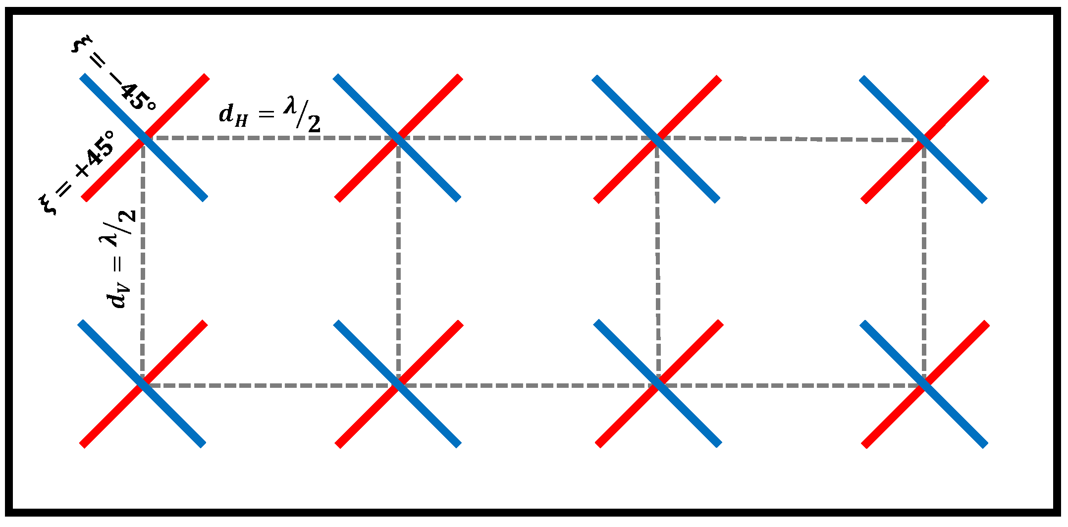
We assume that the BS is equipped by a single-panel Uniform Planar Array (UPA) per each of the three sectors. Each UPA of the BS has $N_{tz}$ antennas along the z-axis and $N_{ty}$ along the y-axis, i.e., $N_t=N_{tz}\times N_{ty}$ total antenna elements. Moreover, $N_t$ also indicates the number of antennas with the same polarization. Antenna elements are uniformly spaced in both dimensions, with distances $d_H$ and $d_V$ in horizontal and vertical direction, respectively. We set the spacing $d_H=d_V=\lambda /2$ where $\lambda =c/f_c$ is the wavelength and c the speed of light. Dual polarization has been taken into account with the parameter P, so each array can be single polarized ($P=1$) or dual polarized ($P=2$), as shown in Figure 2. We denote with $s=(0,1,2)$ the sector index, the UPA with $s=0$ lies on the $yz$-plane (broadside to $\theta ={90}^{\circ }$, $\varphi =0^{\circ }$), the UPAs with $s=1$ and $s=2$ are broadside to ($\theta ={90}^{\circ },\varphi ={120}^{\circ }$) and ($\theta ={90}^{\circ },\varphi ={240}^{\circ }$), respectively.

Given a Zenith of Departure (ZOD) $\theta$ and an Azimuth of Departure (AOD) $\varphi$ in the GCS (Global coordinate system), we need first to convert them into LCS (Local coordinate system) through the mapping:

$$\begin{array}{c}{\theta }^{\prime }=\theta \hfill \\ {\varphi }^{\prime }=\varphi -s{120}^{\circ }\hfill \end{array}$$

(9)

where ${\theta }^{\prime }$ and ${\varphi }^{\prime }$ are the ZoD and AoD in LCS, respectively. We can first write the $N_{tz}\times 1$ steering vector (SV) of the Uniform Linear Array (ULA) on z-axis ${\mathbf{a}}_z\left({\theta }^{\prime }\right)$:

$${\mathbf{a}}_z\left({\theta }^{\prime }\right)={\left[1,e^{j\pi cos{\theta }^{\prime }},\dots ,e^{j\pi (N_{tz}-1)cos{\theta }^{\prime }}\right]}^T$$

(10)

while we denote with ${\mathbf{a}}_{y,s}({\theta }^{\prime },{\varphi }^{\prime })$ the $N_{ty}\times 1$ SV of the generic ULA that lies on the y-axis for $s=0$:

$${\mathbf{a}}^{y,s}({\theta }^{\prime },{\varphi }^{\prime })=\left[\begin{array}{c}1\\ e^{j\pi sin{\theta }^{\prime }sin{\varphi }^{\prime }}\\ ⋮\\ e^{j\pi (N_{ty}-1)sin{\theta }^{\prime }sin{\varphi }^{\prime }}\end{array}\right]$$

(11)

for $s\ne 0$, ${\mathbf{a}}_{y,s}({\theta }^{\prime },{\varphi }^{\prime })$ is rotated of $\pm {120}^{\circ }$. Finally, we can express the $N_t\times 1$ SV for each UPA at the BS as the Kronecker product of the 2 SV’s along each axis:

$${\mathbf{a}}_{tx,s}({\theta }^{\prime },{\varphi }^{\prime })={\mathbf{a}}_z\left({\theta }^{\prime }\right)\otimes {\mathbf{a}}_{y,s}({\theta }^{\prime },{\varphi }^{\prime }).$$

(12)

The 3-D radiation power pattern of each antenna element $A({\theta }^{\prime },{\varphi }^{\prime })$ (adopted for the antenna elements of each array of the BS) is evaluated in LCS (Table 7.3-1 of [21]). It can be expressed in terms of the vertical cut $A_{dB}^{\prime }({\theta }^{\prime },{\varphi }^{\prime }=0^{\circ })$ and horizontal cut $A_{dB}^{\prime }({\theta }^{\prime }={90}^{\circ },{\varphi }^{\prime })$, as follows:

$$A_{dB}^{\prime }({\theta }^{\prime },{\varphi }^{\prime })=-\min \{-(A_{dB}^{\prime }({\theta }^{\prime },{\varphi }^{\prime }=0^{\circ })+A_{dB}^{\prime }({\theta }^{\prime }={90}^{\circ },{\varphi }^{\prime })),A_{max}\}$$

(13)

where $A_{max}=30$ dB is the maximum attenuation. The vertical cut is obtained by fixing ${\varphi }^{\prime }$ to $0^{\circ }$:

$$A_{dB}^{\prime }({\theta }^{\prime },{\varphi }^{\prime }=0^{\circ })=-\min \left\{12{\left(\frac{{\theta }^{\prime }-{90}^{\circ }}{{\theta }_{3dB}}\right)}^2,SL{A}_V\right\}\left[\mathrm{dB}\right]$$

(14)

with ${\theta }_{3dB}={65}^{\circ }$, ${\theta }^{\prime }\in [0^{\circ },{180}^{\circ }]$ and $SL{A}_V=30$ dB is the side-lobe attenuation in the vertical direction. The horizontal cut is obtained by fixing ${\theta }^{\prime }$ to ${90}^{\circ }$:

$$A_{dB}^{\prime }({\theta }^{\prime }={90}^{\circ },{\varphi }^{\prime })=\min \left\{12{\left(\frac{{\varphi }^{\prime }}{{\varphi }_{3dB}}\right)}^2,A_{\max }\right\}\left[\mathrm{dB}\right]$$

(15)

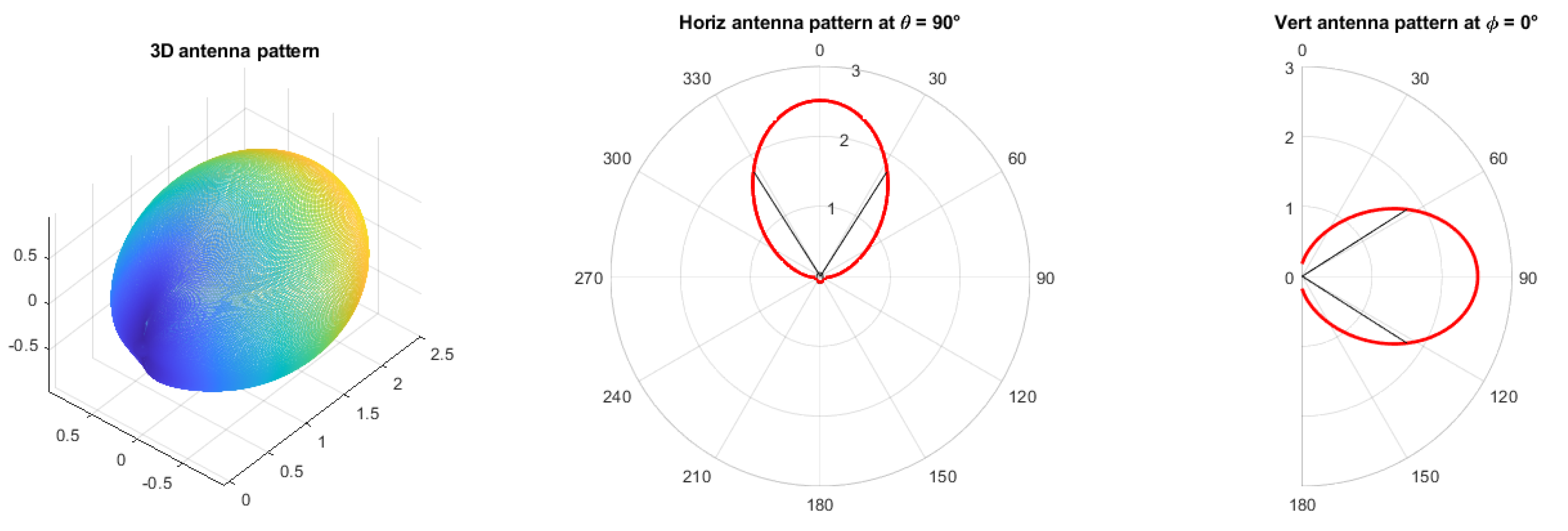
with ${\varphi }_{3dB}={65}^{\circ }$ and ${\theta }^{\prime }\in [-{180}^{\circ },{180}^{\circ }]$. The maximum directional gain of an antenna element $G_{E,\max }$ is equal to 8 dBi. Figure 3 shows in linear scale the 3-D representation, the horizontal cut for a fixed angle $\theta ={90}^{\circ }$, and the vertical cut with a fixed angle $\varphi =0^{\circ }$, respectively, for the 3GPP antenna element radiation pattern.

We select the “Model-2” of the polarized antenna modelling described in Section 7.3.2 of [21]. In general, the relationship between radiation field and power pattern is given by:

$$A^{\prime }({\theta }^{\prime },{\varphi }^{\prime })=|F_{tx,{\theta }^{\prime }}^{\prime }({\theta }^{\prime },{\varphi }^{\prime }){|}^2+{|F_{tx,{\varphi }^{\prime }}^{\prime }({\theta }^{\prime },{\varphi }^{\prime })|}^2$$

(16)

where $F_{tx,{\theta }^{\prime }}^{\prime }({\theta }^{\prime },{\varphi }^{\prime })$ and $F_{tx,{\varphi }^{\prime }}^{\prime }({\theta }^{\prime },{\varphi }^{\prime })$ are the vertical and horizontal polarized field components in LCS, respectively. For the described scenario at the BS, the polarized field components are the same in LCS and GCS. In case of a single polarized antenna (purely vertically polarized antenna), we have

$$F_{tx,\theta }(\theta ,\varphi )=F_{tx,{\theta }^{\prime }}^{\prime }({\theta }^{\prime },{\varphi }^{\prime })=\sqrt{A^{\prime }({\theta }^{\prime },{\varphi }^{\prime })}$$

(17)

i.e., only the vertical polarized field component $F_{tx,\theta }(\theta ,\varphi )$ is active while $F_{tx,\varphi }(\theta ,\varphi )=0$. In case of dual polarization, we have:

$$\begin{array}{c}{F}_{tx,\theta }(\theta ,\varphi )=F_{tx,{\theta }^{\prime }}^{\prime }({\theta }^{\prime },{\varphi }^{\prime })=\sqrt{A^{\prime }({\theta }^{\prime },{\varphi }^{\prime })}cos\left(\xi \right)\hfill \\ F_{tx,\varphi }(\theta ,\varphi )=F_{tx,{\varphi }^{\prime }}^{\prime }({\theta }^{\prime },{\varphi }^{\prime })=\sqrt{A^{\prime }({\theta }^{\prime },{\varphi }^{\prime })}sin\left(\xi \right)\hfill \end{array}$$

(18)

where $\xi$ is the polarization slant angle and $\xi =\pm {45}^{\circ }$ corresponds to a pair of cross polarized antenna elements.

2.2.2. UT Antenna and Array Model

Once all UTs locations are generated, each UT is given a random array orientation. The orientation of an array with respect to the GCS is defined by a set of three angles $(\alpha ,\beta ,$ and $\gamma )$ that fully describe an arbitrary 3-D rotation, where $\alpha$ represents the bearing angle, $\beta$ the downtilt angle, and $\gamma$ the slant angle. The following distributions are assumed:

$$\begin{array}{c}\alpha \sim \mathcal{U}(-{180}^{\circ },+{180}^{\circ })\hfill \\ \beta \sim \mathcal{N}({\mu }_{\beta },{\sigma }_{\beta }^2)\hfill \\ \gamma \sim \mathcal{N}({\mu }_{\gamma },{\sigma }_{\gamma }^2)\hfill \end{array}$$

(19)

where N denotes a normal distribution with ${\mu }_{\beta }={\mu }_{\gamma }=0$ and ${\sigma }_{\beta }^2={\sigma }_{\gamma }^2={36}^{\circ }$. We assume that each UT can also be equipped with a Uniform Planar Array (UPA) with $N_{rz}$ antennas along the z-axis and $N_{ry}$ along the y-axis when $\alpha =\beta =\gamma =0^{\circ }$, i.e., $N_r=N_{rz}\times N_{ry}$ is also the number of antenna with the same polarization. Antenna elements have the same $\lambda /2$ spacing of the BS along both directions and can be single or dual polarized. Given a Zenith of Departure (ZoA) $\theta$ and an Azimuth of Departure (AoA) $\varphi$ in the GCS, we need first to convert into LCS through the following relationship:

$${\theta }^{\prime }(\alpha ,\beta ,\gamma ;\theta ,\varphi )=\mathrm{acos}(cos\beta cos\gamma cos\theta +(sin\beta cos\gamma cos(\varphi -\alpha )-sin\gamma sin(\varphi -\alpha ))\sin \theta )$$

(20)

$$\begin{array}{c}\hfill {\varphi }^{\prime }(\alpha ,\beta ,\gamma ;\theta ,\varphi )=\\ \hfill =arg\left(\begin{array}{c}(cos\beta sin\theta cos(\varphi -\alpha )-sin\beta cos\theta )+\\ +j(cos\beta sin\gamma cos\theta +(sin\beta sin\gamma cos(\varphi -\alpha ))+cos\gamma sin(\varphi -\alpha \left)\right)sin\theta )\end{array}\right)\end{array}$$

(21)

the $N_r\times 1$ SV for the UPA at the UT can be expressed as:

$${\mathbf{a}}_{rx}({\theta }^{\prime },{\varphi }^{\prime })={\mathbf{a}}_z\left({\theta }^{\prime }\right)\otimes {\mathbf{a}}_y({\theta }^{\prime },{\varphi }^{\prime })$$

(22)

where ${\mathbf{a}}_z\left({\theta }^{\prime }\right)$ and ${\mathbf{a}}_y({\theta }^{\prime },{\varphi }^{\prime })$ are computed according to (10) and (11) with ${\theta }^{\prime }$ computed as in (20) and ${\varphi }^{\prime }$ as in (21). We assume that the antenna elements of the array of each UT are half-wave dipoles that are aligned along the z-axis when $\alpha =\beta =\gamma =0$. The radiation power pattern can be expressed as:

$$B^{\prime }\left({\theta }^{\prime }\right)=\frac{{cos}^2\left(\frac{\pi }{2}cos{\theta }^{\prime }\right)}{{sin}^2{\theta }^{\prime }}$$

(23)

$$G_{E,max}=5\mathrm{dBi}.$$

(24)

Due to the fact that the UT array experiences a random 3-D rotation, we need to relate the polarized field components $F_{rx,\theta }\left(\theta \right)$, $F_{rx,\varphi }\left(\theta \right)$ in the GCS, with the components $F_{rx,{\theta }^{\prime }}\left({\theta }^{\prime }\right)$, $F_{rx,{\varphi }^{\prime }}\left({\theta }^{\prime }\right)$ in the LCS through:

$$\left(\begin{array}{c}{F}_{rx,\theta }(\theta ,\varphi )\\ F_{rx,\varphi }(\theta ,\varphi )\end{array}\right)=\left(\begin{array}{cc}+\cos \psi & -\sin \psi \\ +\sin \psi & +\cos \psi \end{array}\right)\left(\begin{array}{c}{F}_{rx{\theta }^{\prime }}^{\prime }\left({\theta }^{\prime }\right)\\ F_{rx,{\varphi }^{\prime }}^{\prime }\left({\theta }^{\prime }\right)\end{array}\right)$$

(25)

where the angle $\psi$ can be computed as:

$$\begin{array}{c}\hfill \psi =arg\left(\begin{array}{c}(sin\gamma cos\theta sin(\varphi -\alpha )+cos\gamma (cos\beta sin\theta -sin\beta cos\theta cos(\varphi -\alpha )\left)\right)+\\ +j(sin\gamma cos(\varphi -\alpha )+sin\beta cos\gamma sin(\varphi -\alpha \left)\right)\end{array}\right)\end{array}.$$

(26)

The same “Model-2” of the polarized antenna modelling of [21] is applied for the UT. In case of single polarized antenna (purely vertically polarized antenna) we have:

$$\begin{array}{c}{F}_{rx,{\theta }^{\prime }}^{\prime }\left({\theta }^{\prime }\right)=\sqrt{B^{\prime }\left({\theta }^{\prime }\right)}\hfill \\ F_{rx,{\varphi }^{\prime }}^{\prime }\left({\theta }^{\prime }\right)=0\hfill \end{array}$$

(27)

while for the case of dual cross-polarization

$$\begin{array}{c}{F}_{rx,{\theta }^{\prime }}^{\prime }\left({\theta }^{\prime }\right)=\sqrt{B^{\prime }\left({\theta }^{\prime }\right)}cos\left(\xi \right)\hfill \\ F_{rx,{\varphi }^{\prime }}^{\prime }\left({\theta }^{\prime }\right)=\sqrt{B^{\prime }\left({\theta }^{\prime }\right)}sin\left(\xi \right)\hfill \end{array}$$

(28)

with $\xi =\pm {45}^{\circ }$, corresponding to a pair of cross-polarized antenna elements. Please note that for each UT it is necessary to apply (25) to the polarized field components in LCS both for single and dual polarization case. In case of single polarized antennas, only the vertical polarized field pattern $F_{rx,\theta }\left(\theta \right)$ will be applied.

3. Link Level Parameters and Channel Coefficient Generation

In this section, we describe all involved link level parameters such as propagation conditions, pathloss, Large Scale Parameters and Small Scale Parameters, and finally we illustrate how to generate channel coefficients for the considered scenario.

3.1. Propagation Conditions and Pathloss Calculation

In this step, we need to evaluate the propagation condition for each BS–UT link by calculating the LOS probability. If UT k is an outdoor user, the parameter $d_{3D}^k$ denotes the pure distance between the BS and the k-th UT in a 3-D coordinate system, while the parameter $d_{2D}^k$ denotes the projection of $d_{3D}^k$ on the x–y plane. The relation between the 2-D distance $d_{2D}^k$ and the 3-D distance $d_{3D}^k$ is given by

$$d_{3D}^k=\sqrt{{\left(d_{2D}^k\right)}^2+{(h_{BS}-h_{UT}^k)}^2}$$

(29)

where $h_{BS}$ is the height of the BS and $h_{UT}^k$ represents the height of k-th user.

Instead, if UT k is an indoor user located inside a building, the parameter $d_{3D}^k$ can be considered as the sum of the two components $d_{3D-out}^k$ and $d_{3D-in}^k$, the former denotes the distance from the BS to the building external wall while the latter denotes the distance from building external wall to the user. The same consideration can be made for $d_{2D}^k$, the projection of $d_{3D}^k$ on the x–y plane, therefore $d_{2D}^k=d_{2D-out}^k+d_{2D-in}^k$ and so the new relation between the 2-D and 3-D distances becomes

$$d_{3D-out}^k+d_{3D-in}^k=\sqrt{{\left(d_{2D-out}^k+d_{2D-in}^k\right)}^2+{\left(h_{BS}-h_{UT}^k\right)}^2}.$$

(30)

Table 7.4.2-1 of [21] provides all details to evaluate the LOS probability $P_{LOS}$ for each scenario. Mainly, the proposed $P_{LOS}$ depends on the 2-D distance between BS and UT, $d_{2D}^k$ for outdoor-to-outdoor (O2O) users and $d_{2D-out}^k$ for outdoor-to-indoor (O2I) ones. As an example, we show how to evaluate the LOS probability for the UMi-Street canyon scenario for the k-th user:

$$P_{LOS}^k=\left\{\begin{array}{cc}1\hfill & d_{2D-out}^k\le 18\mathrm{m}\hfill \\ \frac{18}{d_{2D-out}^k}+exp\left(-\frac{d_{2D-out}^k}{36}\right)\left(1-\frac{18}{d_{2D-out}^k}\right)\hfill & d_{2D-out}^k>18\mathrm{m}\hfill \end{array}\right.$$

(31)

for UMi and UMa scenarios, the LOS probability is 1 for distances smaller than 18 m, and decreases with the distance above this threshold.

According to the propagation conditions described in the previous step, here we calculate the path loss (PL) for each BS–UT link. Table 7.4.1-1 of [21] depicts the formulae for PL evaluation, for UMi and UMa in both cases, LOS and NLOS. Unlike the LOS probability, the path loss is mainly dependent on the 3-D distance between BS and UT, and the carrier frequency $f_c$. In (32) it is shown, as an example, how to evaluate the path loss for the UMi-Street canyon scenario for the k-th user in the case of LOS presence:

$$P{L}_{LOS}^k=\left\{\begin{array}{cc}P{L}_1\hfill & 10\mathrm{m}\le d_{2D}^k\le d_{BP}^k\hfill \\ P{L}_2\hfill & d_{BP}^k<d_{2D}^k\le 5\mathrm{km}\hfill \end{array}\right.$$

(32)

with

$$\begin{array}{c}P{L}_1=32.4+21{log}_{10}\left(d_{3D}^k\right)+20{log}_{10}\left(f_c\right)\hfill \\ P{L}_2=32.4+40{log}_{10}\left(d_{3D}^k\right)+20{log}_{10}\left(f_c\right)-9.5{log}_{10}\left[{\left(d_{BP}^k\right)}^2+{(h_{BS}-h_{UT}^k)}^2\right]\hfill \end{array}$$

(33)

Moreover, $d_{BP}^k$ is the breakpoint distance for the k-th user (Table 7.4.1-1 of [21]), $h_{BS}$ is the height of the base station, while $h_{UT}^k$ represents the height of the k-th user, both expressed in meters, and $f_c$ is the carrier frequency in $Hz$. For indoor users, additional losses are added by taking into account the walls of the building and the losses inside the building as follows

$$P{L}^{ind}=P{L}_b+P{L}_{tw}+P{L}_{in}+\mathcal{N}(0,{\sigma }_P^2)$$

(34)

where $P{L}_b$ is the basic outdoor path loss, $P{L}_{tw}$ is the building penetration loss through the external wall, $P{L}_{in}$ describes the inside loss dependent on the depth into the building, and ${\sigma }_P$ represents the standard deviation for the penetration loss. In [21], it is suggested to calculate $P{L}_{tw}$ by considering $70\%$ of concrete and $30\%$ of glass, while $P{L}_{in}$ is a function of the 2-D distance between the user and the internal wall of the building. All the above parameters are listed in [21], along with the shadowing standard deviation ${\sigma }_{SF}$ for each scenario.

3.2. Large Scale Parameters

In this step, we generate the Large Scale Parameters (LSPs), e.g., all the per-link parameters useful to describe the link behavior between transmitter and receiver. We have seven LSPs for LOS link and six for NLOS case: Delay Spread (DS), angular spreads of departure and arrival in both directions azimuth and zenith (ASA, ASD, ZSA, and ZSD), Ricean K-factor (only of LOS links, $K_R$), and shadow fading ${\sigma }_{SF}$. Table 7.5-6 of [21] provides the means and the variances in logarithmic scale of all these parameters, i.e., all the LSPs are lognormal random variables. The LSPs are generally correlated among them with different kinds of correlations: intra-UT correlation (parameters correlation in the same link) and inter-UT correlation (for different links and can be intra-cell and inter-cell). If we have M LSPs ($M=7$ for a LOS link and $M=6$ in the NLOS case) and a total of K users, and if we assume to take into account both intra- and inter-user correlations, there is a total of $M·K$ parameters to generate and the total correlation matrix has size $MK\times MK$. Undoubtedly, if hundreds of links in system level simulation are considered, the computation of LSPs will be extremely large. WINNER II [23] proposes to calculate inter-UT correlation first and then the intra-UT correlation.

• The inter-UT correlation is calculated by generating a 2-D rectangular mesh based on the UT location for each of the M LSPs. For each mesh grid, M standard normally distributed random variables, which correspond to M LSPs, are assigned and filtered by their corresponding 2-D FIR filter separately. In the following formula, we can see the general expression of the impulse response $h^m\left(d\right)$ of the filter for the m-th LSP

  $$h^m\left(d\right)=exp\left(-\frac{d}{d_{corr}^m}\right)$$

  (35)

  where d is the distance and $d_{corr}^m$ represents the correlation distance of the m-th parameter. If a dense 2-D spatial sampling is applied to each mesh grid, this filtering operation becomes computationally very expensive. Given also that, according to [21], links of UTs on different floors are uncorrelated, we decided not to take into account inter-user correlation.
• Intra-UT correlation is taken into account as follows: for each UT, the M correlated parameters can be obtained by the linear transformation

  $$\tilde{\mathbf{s}}=\sqrt{C_{xx}\left(0\right)}\zeta$$

  (36)

  where $C_{xx}\left(0\right)$ is the $M\times M$ intra-user inter-parameter correlation matrix (which can be obtained from Table 7.5-6 of [21]), $\zeta \sim \mathcal{N}(\mathbf{0},\mathbf{I})$ is a standard normal random vector (all elements are independent zero-mean random variables with unitary variance), and $\tilde{\mathbf{s}}$ is the vector of correlated normal random variables. The final LSPs can be obtained as [41]:

  $$\begin{array}{cc}{10}^{\mathcal{N}({\mu }_x,{\sigma }_x{\tilde{s}}_m)}\hfill & \mathrm{for}\mathrm{DS},\mathrm{ASA},\mathrm{ASD},\mathrm{ZSA},\mathrm{and}\mathrm{ZSD}\hfill \\ {10}^{\mathcal{N}\left({\mu }_x,\frac{{\sigma }_x{\tilde{s}}_m}{10}\right)}\hfill & \mathrm{for}\mathrm{SF}\mathrm{and}\mathrm{K}\hfill \end{array}$$

  (37)

  where ${\mu }_x$ and ${\sigma }_x$ are proper mean and standard deviation, respectively, of the parameter x from Table 7.5-6 of [21].

Finally, in this LSP step, we generate the number of cluster $N_{cl}$ per link and the total number of rays per cluster $M_{ray}$. Both parameters are listed in Table 7.5-6 of [21] for LOS, NLOS, and O2I cases. For UMi, $N_{cl}=12$ for LOS and O2I, while $N_{cl}=19$ for NLOS; $M_{ray}=20$ for all three case.

3.3. Small Scale Parameters

In this step we consider the Small Scale Parameters (SSPs), i.e., cluster parameters such as delay, power, and angular spread, and intra-cluster or ray parameters, such as angle of departure and arrival and cross polarization power ratio.

3.3.1. Cluster Delays

The first SSP is the cluster delay. We need to generate with exponential delay distribution the propagation delays for each cluster as follows

$${\tau }_n^{\prime }=-r_{\tau }DSln\left(X_n\right)$$

(38)

where $r_{\tau }$ is the delay scaling, $DS$ is the delay spread of the link and $X_n\sim U(0,1)$ where n is the cluster index. For the final delay set, we need to normalize and sort the delay vector

$${\tau }_n=\mathrm{sort}({\tau }_n^{\prime }-min\left({\tau }_n^{\prime }\right)).$$

(39)

In case of LOS condition, additional scaling of delays is needed to compensate the effect of LOS peak addition to the delay spread. To scale the delay set, we use a constant $C_{\tau }$: ${\tau }_n^{LOS}={\tau }_n/C_{\tau }$ where $C_{\tau }=0.7705-0.0433K_r+0.0002K_r^2+0.000017K_r^3$ and $K_r$ is the Ricean K-factor in dB.

3.3.2. Cluster Powers

The second set of parameters is the cluster power, denoted by $P_n$. For each cluster, we first compute

$$P_n^{\prime }=exp\left(-{\tau }_n\frac{r_{\tau }-1}{r_{\tau }DS}\right){10}^{-Z_n/10}$$

(40)

where $Z_n\sim \mathcal{N}(0,{\zeta }^2)$, $\zeta$ represents the per-cluster shadowing and can be found in Table 7.5-6 of [21]. In order to have the sum of the cluster powers equal to one, we divide the previous power set $P_n^{\prime }$ by the total power and so we obtain the normalized set $P_n$

$$P_n=\frac{P_n^{\prime }}{{\sum }_{n=1}^{N_{cl}}{P}_n^{\prime }}.$$

(41)

In the case of LOS condition, an additional specular component is added to the first cluster $P_{1,LOS}=K_R/(K_R+1)$, where $K_R$ is the Ricean K-factor converted to linear scale. Therefore, in the case of LOS, we need to change the normalization strategy as follows:

$$P_n=\frac{1}{K_R+1}\frac{P_n^{\prime }}{{\sum }_{n=1}^{N_{c}l}{P}_n^{\prime }}+\delta (n-1)P_{1,LOS}.$$

(42)

After the normalization, we remove the clusters with less than $-25$ dB power compared to the maximum cluster power. The scaling factor does not need to be changed after cluster elimination. Once we have the cluster powers $P_n$, we assign the power to each ray by splitting $P_n$ equally over the total number of rays, so $P_{n,m}=P_n/M_{ray}$, where $n=1,\cdots ,N_{cl}$ is the cluster index and $m=1,\cdots ,M_{ray}$ is the ray index.

3.3.3. Arrival and Departure Angles for Both Azimuth and Elevation

In this step, we generate the per ray angles of arrival and departure in both azimuth and elevation.

AOAs and AODs Generation

The Power Angular Spectrum (PAS) reflects the power distribution in different direction and determines the spatial correlation properties of the channel. The composite PAS in azimuth of all clusters is modelled as a wrapped Gaussian distribution. We show how to generate AOAs; the procedure to generate AODs is very similar. AOAs are generated by applying the inverse Gaussian distribution with cluster average power $P_n$ and Root Mean Square (RMS) Azimuth Spread of Arrival (ASA):

$${\tilde{\varphi }}_{n,AOA}=\frac{2ASA\sqrt{-ln(P_n/\max \left(P_n\right))}}{1.4C_{\varphi }}$$

(43)

with $C_{\varphi }$ defined as:

$$C_{\varphi }=\left\{\begin{array}{cc}{C}_{\varphi }^{NLOS}(1.1035-0.028K-0.002K^2+0.0001K^3)\hfill & \mathrm{for}\mathit{LOS}\hfill \\ C_{\varphi }^{NLOS}\hfill & \mathrm{for}\mathit{NLOS}\hfill \end{array}\right.$$

(44)

where $C_{\varphi }^{NLOS}$ can be found in Table 7.5-2 of [21]. In the case of LOS contribution, $C_{\varphi }$ also depends on the Ricean factor K. Cluster angles ${\varphi }_{n,AOA}$ can be generated as

$${\varphi }_{n,AOA}=\left\{\begin{array}{cc}{X}_n{\tilde{\varphi }}_{n,AOA}+Y_n+{\varphi }_{LOS,AOA}\hfill & \mathrm{for}\mathit{NLOS}\hfill \\ X_n{\tilde{\varphi }}_{n,AOA}+Y_n-X_1{\tilde{\varphi }}_{1,AOA}-Y_1+{\varphi }_{LOS,AOA}\hfill & \mathrm{for}\mathit{LOS}\hfill \end{array}\right.$$

(45)

where $X_n$ is a discrete random variable uniformly distributed in the set $\{-1,1\}$ and $Y_n\sim \mathcal{N}(0,{(ASA/7)}^2)$ is used to introduce random variation. In the case of LOS link, the first cluster has angle equal to the LOS one ${\varphi }_{1,AOA}={\varphi }_{LOS,AOA}$.

Finally, for ray angles we need to add offset angles to the azimuth cluster angle as follows:

$${\varphi }_{n,m,AOA}={\varphi }_{n,AOA}+C_{ASA}{\alpha }_m$$

(46)

where $C_{ASA}$ is the cluster-wise RMS azimuth spread of arrival and ${\alpha }_m$ is the per-ray offset, which can be found in Table 7.5-3 of [21]. AODs generation follows the same procedure from (43) to (46) by substituting ASA with Azimuth Spread of Departure (ASD) and $C_{ASA}$ with the cluster-wise RMS azimuth spread of departure $C_{ASD}$.

ZOAs and ZODs Generation

The composite PAS in zenith of all clusters is modelled as a Laplacian distribution. ZOAs are generated by applying the inverse Laplacian distribution with cluster average power $P_n$ and RMS Zenith Spread of Arrival (ZSA):

$${\tilde{\theta }}_{n,ZOA}=-\frac{ZSAln(P_n/max\left(P_n\right))}{C_{\theta }}$$

(47)

with $C_{\theta }$ defined as:

$$C_{\theta }=\left\{\begin{array}{cc}{C}_{\theta }^{NLOS}(1.3086+0.0339K-0.{0077}^2+0.0002K^3)\hfill & \mathrm{for}\mathit{LOS}\hfill \\ C_{\theta }^{NLOS}\hfill & \mathrm{for}\mathit{NLOS}\hfill \end{array}\right.$$

(48)

where $C_{\theta }^{NLOS}$ can be found in Table 7.5-4 of [21]. In the case of LOS contribution $C_{\theta }$ also depends on the Ricean factor K. Cluster angles ${\theta }_{n,ZOA}$ can be generated as

$${\theta }_{n,ZOA}=\left\{\begin{array}{cc}{X}_n{\tilde{\theta }}_{n,ZOA}+Y_n+{\overline{\theta }}_{ZOA}\hfill & \mathrm{for}\mathit{NLOS}\hfill \\ X_n{\tilde{\theta }}_{n,ZOA}+Y_n-X_1{\tilde{\theta }}_{1,ZOA}-Y_1+{\theta }_{LOS,ZOA}\hfill & \mathrm{for}\mathit{LOS}\hfill \end{array}\right.$$

(49)

where ${\overline{\theta }}_{ZOA}={90}^{\circ }$ if the BS–UT link is O2I (the UT is indoor) and ${\overline{\theta }}_{ZOA}={\overline{\theta }}_{LOS,ZOA}$; otherwise, $X_n$ is a discrete random variable uniformly distributed in the set $\{-1,1\}$ and $Y_n\sim \mathcal{N}(0,{(ZSA/7)}^2)$ is used to introduce random variation. In the case of LOS link, the first cluster has angle equal to the LOS one ${\theta }_{1,ZOA}={\theta }_{LOS,ZOA}$.

Finally, for ray angles we need to add offset angles to the zenith cluster angle as follows:

$${\theta }_{n,m,ZOA}={\theta }_{n,ZOA}+C_{ZSA}{\alpha }_m$$

(50)

where $C_{ZSA}$ is the cluster-wise RMS zenith spread of arrival and ${\alpha }_m$ is the per-ray offset.

ZODs generation follows a similar procedure as for ZOA. First, generate ${\tilde{\theta }}_{n,ZOD}$ with Zenith Spread of Departure (ZSD) instead of ZSA, then replace (49) with:

$${\theta }_{n,ZOD}=\left\{\begin{array}{cc}{X}_n{\tilde{\theta }}_{n,ZOD}+Y_n+{\theta }_{LOS,ZOD}+{\mu }_{offset,ZOD}\hfill & \mathrm{for}\mathit{NLOS}\hfill \\ X_n{\tilde{\theta }}_{n,ZOD}+Y_n-X_1{\tilde{\theta }}_{1,ZOD}-Y_1+{\theta }_{LOS,ZOD}\hfill & \mathrm{for}\mathit{LOS}\hfill \end{array}\right.$$

(51)

where $X_n$ is a discrete random variable uniformly distributed in the set $\{-1,1\}$, $Y_n\sim \mathcal{N}(0,{(ZSD/7)}^2)$, and ${\mu }_{offset,ZOD}$ is a modified factor related to the BS–UT distance and antenna height in case of NLOS conditions and is given in Tables 7.5-7 and 7.5-8 of [21], respectively. Finally, (50) is replaced by:

$${\theta }_{n,m,ZOD}={\theta }_{n,ZOD}+(3/8)\left({10}^{{\mu }_{lgZSD}}\right){\alpha }_m$$

(52)

where ${\mu }_{lgZSD}$ is the mean of the ZSD log-normal distribution.

Coupling of Rays within a Cluster

Once we have all the per-ray angles, we need to random couple them within a cluster in the following way:

• Couple randomly AOD angles ${\varphi }_{n,m,AOD}$ to AOA ${\varphi }_{n,m,AOA}$ within a cluster n;
• Couple randomly ZOD angles ${\theta }_{n,m,ZOD}$ to ZOA ${\theta }_{n,m,ZOA}$ angles within a cluster n;
• Couple randomly AOD angles ${\varphi }_{n,m,AOD}$ with ZOD angles ${\theta }_{n,m,ZOD}$ within a cluster n.

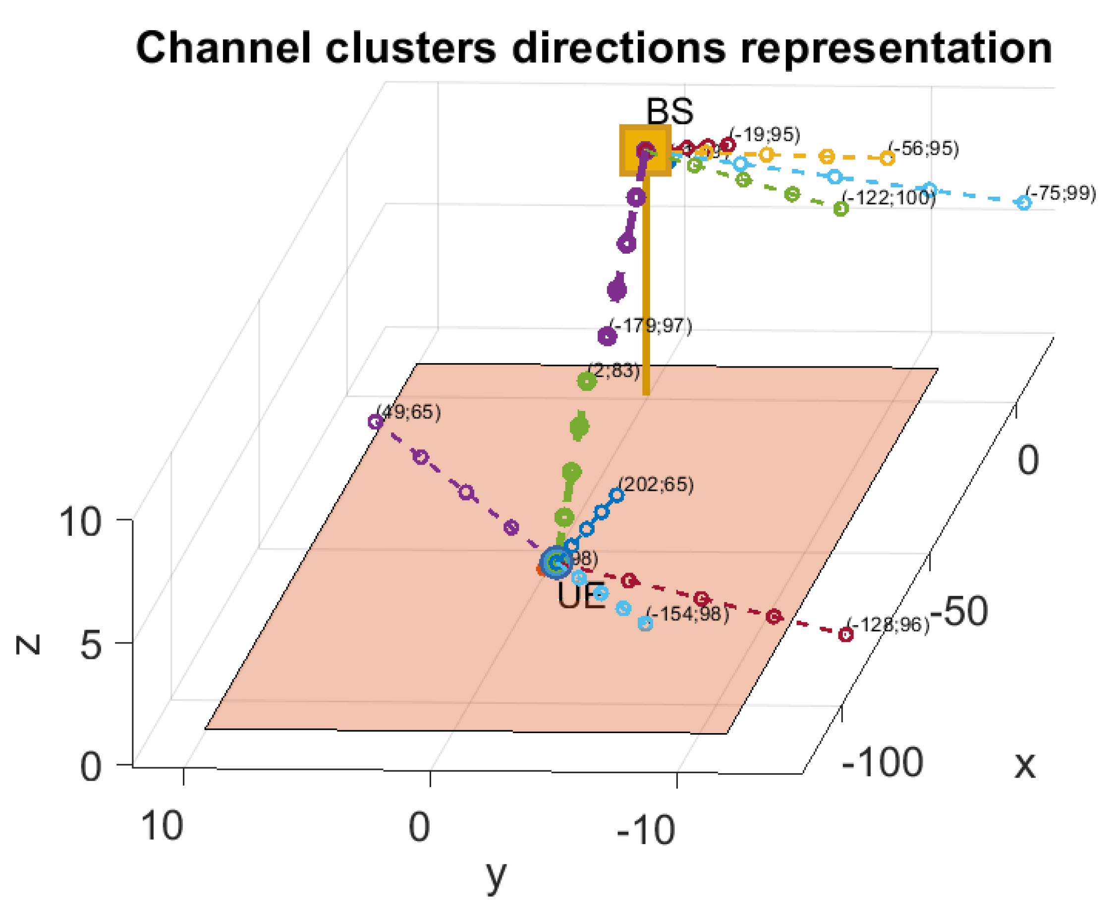
where $n=1,\cdots ,N_{cl}$ and $m=1,\cdots ,M_{ray}$. Figure 4 shows cluster angles ${\theta }_{n,ZOD},{\varphi }_{n,AOD}$ at the BS and ${\theta }_{n,ZOA},{\varphi }_{n,AOA}$ at the UT for a particular channel realization, in the case of LOS link.

3.3.4. Cross Polarization Power Ratio

The last step for small scale parameters is to generate the cross polarization power ratios (XPR) for each ray m of each cluster n. XPR is log-Normal distributed as follows

$${\mathcal{K}}_{n,m}={10}^{X/10}$$

(53)

where $X\sim \mathcal{N}({\mu }_{XPR},{\sigma }_{XPR}^2)$ is Gaussian distributed, $n=1,\cdots ,N_{cl}$ and $m=1,\cdots ,M_{ray}$. The XPR average ${\mu }_{XPR}$ and variance ${\sigma }_{XPR}$ are listed in Table 7.5-6 of [21] for each scenario.

3.4. Coefficient Generation

Before channel coefficient generation, we need to randomly draw the initial phases $\left\{{\Phi }_{n,m}^{\theta \theta }{\Phi }_{n,m}^{\theta \varphi }{\Phi }_{n,m}^{\varphi \theta }{\Phi }_{n,m}^{\varphi \varphi }\right\}$. The initial phases are uniformly distributed in the range $(-\pi ,\pi )$. The final time-invariant channel model expression will be a matrix-valued function of the variable $\tau$.

In case of single-polarized antenna elements at both the transmitter and receiver, we define for each cluster n and ray m the scalar term $g_{n,m}$ as:

$$g_{n,m}=F_{rx,\theta }\left({\theta }_{n,m,ZOA},{\varphi }_{n,m,AOA}\right)exp\left(j{\Phi }_{n,m}^{\theta \theta }\right)F_{tx,\theta }\left({\theta }_{n,m,ZOD},{\varphi }_{n,m,AOD}\right)$$

(54)

we obtain the following $N_r\times N_t$ channel matrix ${\mathbf{H}}_{n,m,s}^{NLOS}$ relative to the cluster n, ray m and sector s:

$${\mathbf{H}}_{n,m,s}^{NLOS}=\sqrt{\frac{P_n}{M_{ray}}}{g}_{n,m}{\mathbf{a}}_{rx}({\theta }_{n,m}^{\prime },{\varphi }_{n,m}^{\prime }){\mathbf{a}}_{tx,s}^H({\theta }_{n,m}^{\prime },{\varphi }_{n,m}^{\prime })$$

(55)

In case of dual cross-polarized pairs of antenna, for each array element at both the transmitter and receiver, we define for each cluster n and ray m the $2\times 2$ matrix ${\mathbf{G}}_{n,m}$ as:

$$\begin{array}{cc}\hfill {\mathbf{G}}_{n,m}=& \left[\begin{array}{cc}{F}_{rx,\theta }^{+\xi }\left({\theta }_{n,m,ZOA}{\varphi }_{n,m,AOA}\right)& F_{rx,\varphi }^{+\xi }\left({\theta }_{n,m,ZOA},{\varphi }_{n,m,AOA}\right)\\ F_{rx,\theta }^{-\xi }\left({\theta }_{n,m,ZOA},{\varphi }_{n,m,AOA}\right)& F_{rx,\varphi }^{-\xi }\left({\theta }_{n,m,ZOA},{\varphi }_{n,m,AOA}\right)\end{array}\right]\left[\begin{array}{cc}exp\left(j{\Phi }_{n,m}^{\theta \theta }\right)& \sqrt{{\mathcal{K}}_{n,m}^{-1}}exp\left(j{\Phi }_{n,m}^{\theta \varphi }\right)\\ \sqrt{{\mathcal{K}}_{n,m}^{-1}}exp\left(j{\Phi }_{n,m}^{\varphi \theta }\right)& exp\left(j{\Phi }_{n,m}^{\varphi \varphi }\right)\end{array}\right]\hfill \\ \hfill & \left[\begin{array}{cc}{F}_{tx,\theta }^{+\xi }\left({\theta }_{n,m,ZOD},{\varphi }_{n,m,AOD}\right)& F_{tx,\theta }^{-\xi }\left({\theta }_{n,m,ZOD},{\varphi }_{n,m,AOD}\right)\\ F_{tx,\varphi }^{+\xi }\left({\theta }_{n,m,ZOD},{\varphi }_{n,m,AOD}\right)& F_{tx,\varphi }^{-\xi }\left({\theta }_{n,m,ZOD},{\varphi }_{n,m,AOD}\right)\end{array}\right]\hfill \end{array}$$

(56)

where the $F^{+\xi }$ ($F^{-\xi }$) indicates the polarized field component with polarization slant angle $+{45}^{\circ }$ ($-{45}^{\circ }$). The channel matrix ${\mathbf{H}}_{n,m,s}^{NLOS}$ relative to cluster n, ray m, and sector s becomes of size $2N_r\times 2N_t$ and can be computed as:

$${\mathbf{H}}_{n,m,s}^{NLOS}=\sqrt{\frac{P_n}{M_{ray}}}\left[{\mathbf{a}}_{rx}({\theta }_{n,m,ZOA}^{\prime },{\varphi }_{n,m,AOA}^{\prime }){\mathbf{a}}_{tx,s}^H({\theta }_{n,m,ZOD}^{\prime },{\varphi }_{n,m,AOD}^{\prime })\right]\otimes {\mathbf{G}}_{n,m}$$

(57)

For the $N_{cl}-2$ weakest clusters, so for $n=3,4,\cdots ,N_{cl}$, all rays belonging to the same cluster n have equal delay ${\tau }_n$. For the two strongest cluster, $n=1$ and $n=2$, rays are spread in delay to three sub-clusters $R_1$, $R_2$ and $R_3$ in the same cluster n, and are mapped as $R_1=\left\{1,2,3,4,5,6,7,8,19,20\right\}$, $R_2=\left\{9,10,11,12,17,18\right\}$ and $R_3=\left\{13,14,15,16\right\}$. For each subcluster a fixed delay offset is applied and a fraction of the cluster power $P_n$, proportional to the number of rays mapped onto it, is assigned. The delays of the sub-clusters are:

$$\begin{array}{c}{\tau }_{n,1}={\tau }_n\hfill \\ {\tau }_{n,2}={\tau }_n+1.28c_{DS}\hfill \\ {\tau }_{n,3}={\tau }_n+2.56c_{DS}\hfill \end{array}$$

(58)

where $c_{DS}$ is the cluster delay spread that can be found in Table 7.5-6 of [21] (e.g., for UMi LOS scenario, $c_{DS}=5$ ns).

Therefore, the total time-invariant channel matrix-valued function for the s-th sector ${\mathbf{H}}_s^{NLOS}\left(\tau \right)$ can be obtained by summing all the matrices from each ray of each cluster in the following way:

$${\mathbf{H}}_s^{NLOS}\left(\tau \right)=\sum _{n=1}^2\sum _{i=1}^3\sum _{m\in R_i}{\mathbf{H}}_{n,m,s}^{NLOS}\delta \left(\tau -{\tau }_{n,i}\right)+\sum _{n=3}^{N_{cl}}\sum _{m=1}^{M_{ray}}{\mathbf{H}}_{n,m,s}^{NLOS}\delta \left(\tau -{\tau }_n\right)$$

(59)

In the case of LOS presence, we define the LOS channel matrix as:

$${\mathbf{H}}_s^{LOS}=\left\{\begin{array}{cc}{g}_{LOS}{\mathbf{a}}_{rx}({\theta }_{LOS,ZOA}^{\prime },{\varphi }_{LOS,AOA}^{\prime }){\mathbf{a}}_{tx,s}^H({\theta }_{LOS,ZOD}^{\prime },{\varphi }_{LOS,AOD}^{\prime })\hfill & \mathrm{for}\mathrm{single}\mathrm{pol}.\hfill \\ \left[{\mathbf{a}}_{rx}({\theta }_{LOS,ZOA}^{\prime },{\varphi }_{LOS,AOA}^{\prime }){\mathbf{a}}_{tx,s}^H({\theta }_{LOS,ZOD}^{\prime },{\varphi }_{LOS,AOD}^{\prime })\right]\otimes {\mathbf{G}}_{LOS}\hfill & \mathrm{for}\mathrm{dual}\mathrm{pol}.\hfill \end{array}\right.$$

(60)

with

$$g_{n,m}=F_{rx,\theta }\left({\theta }_{LOS,ZOA},{\varphi }_{LOS,AOA}\right)F_{tx,\theta }\left({\theta }_{LOS,ZOD},{\varphi }_{LOS,AOD}\right)$$

(61)

and

$$\begin{array}{cc}\hfill {\mathbf{G}}_{n,m}=& \left[\begin{array}{cc}{F}_{rx,\theta }^{+\xi }\left({\theta }_{LOS,ZOA},{\varphi }_{LOS,AOA}\right)& F_{rx,\varphi }^{+\xi }\left({\theta }_{LOS,ZOA},{\varphi }_{LOS,AOA}\right)\\ F_{rx,\theta }^{-\xi }\left({\theta }_{LOS,ZOA},{\varphi }_{LOS,AOA}\right)& F_{rx,\varphi }^{-\xi }\left({\theta }_{LOS,ZOA},{\varphi }_{LOS,AOA}\right)\end{array}\right]\left[\begin{array}{cc}1& 0\\ 0& -1\end{array}\right]\hfill \\ \hfill & \left[\begin{array}{cc}{F}_{tx,\theta }^{+\xi }\left({\theta }_{LOS,ZOD},{\varphi }_{LOS,AOD}\right)& F_{tx,\theta }^{-\xi }\left({\theta }_{LOS,ZOD},{\varphi }_{LOS,AOD}\right)\\ F_{tx,\varphi }^{+\xi }\left({\theta }_{LOS,ZOD},{\varphi }_{LOS,AOD}\right)& F_{tx,\varphi }^{-\xi }\left({\theta }_{LOS,ZOD},{\varphi }_{LOS,AOD}\right)\end{array}\right]\hfill \end{array}$$

(62)

In this case, the final matrix-valued channel impulse response is given by adding the the NLOS and LOS component and scaling both terms by the Ricean factor $K_R$. The LOS component is associated with the shortest possible delay of all ${\tau }_n$, i.e., ${\tau }_1$:

$${\mathbf{H}}_s^{LOS}\left(\tau \right)=\sqrt{\frac{1}{K_R+1}}{\mathbf{H}}_s^{NLOS}\left(\tau \right)+\sqrt{\frac{K_R}{K_R+1}}{\mathbf{H}}_s^{LOS}(\tau -{\tau }_1).$$

(63)

As final step, we apply path loss and shadowing for all the channel coefficients. After selecting the sampling frequency $f_s$, the channel impulse response can be sampled and the total number of necessary taps $N_{taps}$ to represent the channel can be computed as:

$$N_{taps}=1+\underset{n}{max}⌊{\tau }_n{f}_s+\frac{1}{2}⌋$$

(64)

the total sampled channel ${\mathbf{\mathscr{H}}}_s$ can be represented as a $N_r\times N_t\times T$ tensor of order 3 per each sector.

4. Multi-User MIMO System Model

Given the scenario described in Section 2, we consider the downlink communication between a single trisectorized BS and K users, and we focus on the precoding and combining scheme as depicted in Figure 5 of an OFDM Multi-User Multi-Layer MIMO system over wideband mmWave channels with Q subcarriers. The BS is equipped with $N_t$ transmitting antennas per sector and each UT with $N_r$ receiving antenna. Firstly, each of the K UTs placed inside the cell is assigned to one of the three sectors, the BS then transmits L data streams simultaneously to each UT, with $L\le N_r\ll N_t$ and $LK\le N_t$. Let ${\mathbf{s}}_k\left(q\right)$ denote the data symbol vector to be transmitted to the k-th user at the subcarrier q and $\mathbb{E}\left[{\mathbf{s}}_k\left(q\right){\mathbf{s}}_k^H\left(q\right)\right]=1/L\mathbf{I}$, therefore, at the BS, $LK$ data-symbols $\mathbf{s}[\left(q\right)={[{\mathbf{s}}_1^T\left(q\right){\mathbf{s}}_2^T\left(q\right)\dots {\mathbf{s}}_K^T\left(q\right)]}^T$ are precoded with a subcarrier-dependent precoder $\mathbf{W}\left(q\right)=[{\mathbf{W}}_1\left(q\right){\mathbf{W}}_2\left(q\right)\dots {\mathbf{W}}_K\left(q\right)]$ of size $N_t\times LK$, where ${\mathbf{W}}_k\left(q\right)$ represents the precoder designed for the k-th user. A sum power constraint is imposed on the total transmission power $P_{tot}$, i.e., $\parallel \mathbf{W}\left(q\right)\parallel \le P_{tot}/Q$. The data symbols are then transformed to the time domain through a $N_{FFT}$-point Inverse Fast-Fourier Transform (IFFT). A cyclic prefix (CP) of length D is then added to the data-symbols. The total transmitted signal at subcarrier q can be written as:

$$\mathbf{x}\left(q\right)=\mathbf{W}\left(q\right)\mathbf{s}\left(q\right)$$

(65)

We assume Time Division Duplexing (TDD) with channel reciprocity and ideal channel state information (CSI) at the BS, i.e., the BS can obtain long-term averaged over the fading CSI for each user. Moreover, users communicate in the same time slot or resource and the BS:

• resorts only to Space Division Multiple Access (SDMA) through precoding techniques;
• is able to process all $KL$ users’ signals, therefore we impose no limitation on the number of RF chains, i.e., the BS is able to employ at least $KL$ parallel precoders.

In our simulation, we generate the $N_r\times N_t\times N_{taps}$ channel tensor ${\mathbf{\mathscr{H}}}_{s,k}$ from sector s of the BS to user k in time domain as described in Section 3, we perform a $N_{FFT}$-point FFT along the 3rd dimension for each RX–TX antenna pair, and we obtain a $N_r\times N_t\times N_{FFT}$ frequency response channel tensor ${\widetilde{\mathbf{\mathscr{H}}}}_{s,k}$, where each $N_r\times N_t$ matrix ${\tilde{\mathbf{H}}}_{s,k}\left(q\right)$ represents the flat MIMO channel of the q-th subband.

After sector selection, the baseband equivalent receiving signal of the k-th user at subcarrier q can be written as follows:

$${\mathbf{y}}_k\left(q\right)={\tilde{\mathbf{H}}}_k\left(q\right)\mathbf{x}\left(q\right)={\tilde{\mathbf{H}}}_k\left(q\right)\sum _{i=1}^K{\mathbf{W}}_i\left(q\right){\mathbf{s}}_i\left(q\right)+{\mathbf{n}}_k\left(q\right)$$

(66)

where ${\mathbf{n}}_k\left(q\right)$ is a length $N_r$ noise vector whose entries are independent and identically distributed according to $\mathcal{CN}(0,{\sigma }_k^2)$ and are spatially white, i.e., $\mathbb{E}\left[{\mathbf{n}}_k\left(q\right){\mathbf{n}}_k^H\left(q\right)\right]={\sigma }_k^2\mathbf{I}$, moreover ${\sigma }_k^2=k_{B}TF\Delta ,\forall k$, where $k_B$ is the Boltzmann constant, T the temperature, F the noise figure, and $\Delta$ the size of the subband or subcarrier spacing (SCS).

4.1. Sector Assignment

Each of the K UTs placed inside the cell must be assigned to one of the three sectors. As the 3-D position of the UTs is not known at the BS, we exploit the channel matrices to evaluate the suitability of a certain UT to be served by the antenna array of a sector, i.e., the link quality between them. If we denote with $\mathcal{U}=\{U_1,U_2,\dots ,U_K\}$ the set of all users to be assigned, and with ${\mathcal{A}}_1,{\mathcal{A}}_2,$ and ${\mathcal{A}}_3$ the set of users assigned to sectors 1, 2, and 3 respectively, a user can only be assigned to one sector, i.e., $(A_i\cap A_j)=⌀$ and $|{\mathcal{A}}_1\cup {\mathcal{A}}_2\cup {\mathcal{A}}_3|=K$, where $\left|\mathcal{X}\right|$ denotes the cardinality of $\mathcal{X}$. Then:

$$U_k\in {\mathcal{A}}_s,s=\underset{j}{\mathrm{argmax}}\sum _q^Q{\parallel {\mathbf{H}}_{k,j}\left(q\right)\parallel }_F^2,j=1,2,3$$

(67)

where ${\parallel ·\parallel }_F^2$ indicates the Frobenius norm. Therefore the user is assigned to the sector whose channel has the highest energy.

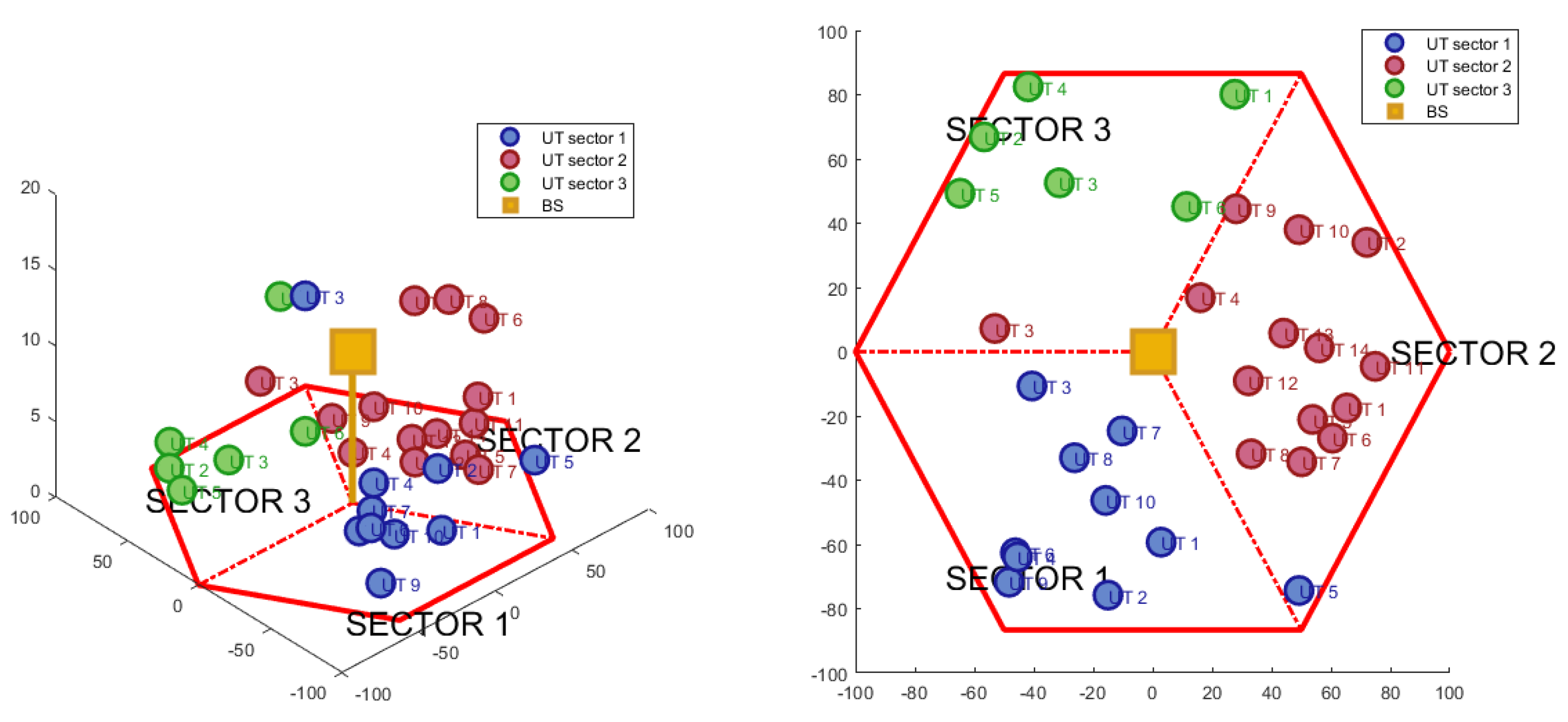
We could expect that the UTs in LOS will be assigned to the same sector as the one covering their x–y coordinates, except for the UTs in the sector borders, where some uncertainty is present. For NLOS UTs, the sector assignment could have even less or no correspondence to the actual placement in the hexagon. An example of the sector assignment result can be seen in Figure 6.

In a real case scenario, for example in 5G NR, the sector assignment is commonly a consequence of the initial access procedure, where the UT chooses the sector depending on the synchronization signal strength that it experiences. Even if this procedure is different from the one considered in our scenario, they both strongly depend on the link quality between the BS and the UT. We reasonably expect that the result of our assignment does not remarkably differ from a real scenario.

4.2. SLNR Precoding and MMSE Combining

For notation simplicity, we omit the subcarrier index q in the following discussions. In order to analyze the performance of a multi-user multi-layer MIMO scheme under the 3GPP 3-D channel model we split the processing at the transmitter and the receiver:

• at the transmitter, we adopt a Signal-to-Leakage-plus-Noise Ratio (SLNR) precoder [17], which is able to minimize the inter-user interference;
• at each UT, we adopt a Minimum Mean Square Error (MMSE) combiner [42], which will minimize the intra-user inter-layer interference.

Given a user k, the interference caused to the other UTs can be defined as the leakage:

$$\sum _{\begin{array}{c}i=1\\ i\ne k\end{array}}^K{\parallel {\tilde{\mathbf{H}}}_i{\mathbf{W}}_k\parallel }_F^2$$

(68)

this leads to the SLNR expression the ratio between the signal power for user k and the noise plus the leakage:

$$SLN{R}_k=\frac{\parallel {\tilde{\mathbf{H}}}_k{\mathbf{W}}_k{\parallel }_F^2}{N_r{\sigma }_k^2+{\sum }_{\begin{array}{c}i=1\\ i\ne k\end{array}}^K{\parallel {\tilde{\mathbf{H}}}_i{\mathbf{W}}_k\parallel }_F^2}.$$

(69)

The SLNR expression can be rewritten as:

$$SLN{R}_k=\frac{\parallel {\tilde{\mathbf{H}}}_k{\mathbf{W}}_k{\parallel }_F^2}{N_r{\sigma }_k^2+{\parallel {\mathbf{Z}}_k{\mathbf{W}}_k\parallel }_F^2}$$

(70)

where:

$${\mathbf{Z}}_k={\left[{\tilde{\mathbf{H}}}_1\cdots {\tilde{\mathbf{H}}}_{k-1}{\tilde{\mathbf{H}}}_{k+1}\right]}^T$$

(71)

is an extended $N_{r}K\times N_t$ channel matrix that only excludes user k. The transmit precoding matrix targeted for user k that maximizes its SLNR is given by

$${\widehat{\mathbf{W}}}_k=\underset{{\mathbf{W}}_k\in {\mathbb{C}}^{N_t\times L}}{\mathrm{argmax}}SLN{R}_k=\underset{{\mathbf{W}}_k\in {\mathbb{C}}^{N_t\times L}}{\mathrm{argmax}}\frac{\parallel {\tilde{\mathbf{H}}}_k{\mathbf{W}}_k{\parallel }_F^2}{N_r{\sigma }_k^2+{\parallel {\mathbf{Z}}_k{\mathbf{W}}_k\parallel }_F^2}$$

(72)

it is shown in [20,43] that the optimal precoder is linked to the solution of the generalized eigenvalue problem

$$\left({\tilde{\mathbf{H}}}_k^H{\tilde{\mathbf{H}}}_k\right)\mathbf{E}=\left(N_r{\sigma }_k^2\mathbf{I}+{\mathbf{Z}}_k^H{\mathbf{Z}}_k\right)\mathbf{E}\Lambda$$

(73)

where $\mathbf{E}=\left[{\mathbf{e}}_1,\dots ,{\mathbf{e}}_{N_t}\right]$ are the eigenvectors and $\Lambda =\mathrm{diag}\left({\left[{\lambda }_1,\dots ,{\lambda }_{N_t}\right]}^T\right)$ the eigenvalues of ${\left(N_r{\sigma }_k^2\mathbf{I}+{\mathbf{Z}}_k^H{\mathbf{Z}}_k\right)}^{-1}{\tilde{\mathbf{H}}}_k^H{\tilde{\mathbf{H}}}_k$, respectively. Then the SLNR precoder is:

$${\mathbf{W}}_k\left[{\mathbf{e}}_1,\dots ,{\mathbf{e}}_L\right]$$

(74)

i.e., ${\mathbf{W}}_k$ is made by the L eigenvectors corresponding to the L largest eigenvalues ${\lambda }_1,\dots ,{\lambda }_L$.

The design of the proper combiner at the UT, which will allow us to minimize the inter-layer interference, requires the definition of the equivalent channel matrix after precoding at the receiver k:

$${\mathbf{P}}_k={\tilde{\mathbf{H}}}_k{\mathbf{W}}_k.$$

(75)

The designed $L\times N_r$ combining matrix ${\mathbf{U}}_k$ is a linear Minimum Mean Square Error (MMSE) receiver, defined as

$${\mathbf{U}}_k={\left({\mathbf{P}}_k^H{\mathbf{P}}_k+\frac{1}{\rho }\mathbf{I}\right)}^{-1}{\mathbf{P}}_k^H$$

(76)

with

$$\rho =\frac{P_{tot}}{QK{N}_r{\sigma }^2}.$$

(77)

The estimated signal vector ${\widehat{\mathbf{s}}}_k$ for UT k after MMSE combining becomes:

$${\widehat{\mathbf{s}}}_k={\mathbf{U}}_k{\tilde{\mathbf{H}}}_k\sum _{i=1}^K{\mathbf{W}}_i{\mathbf{s}}_i+{\mathbf{U}}_k{\mathbf{n}}_k$$

(78)

By recalling the structure of precoding and combining matrices ${\mathbf{W}}_k$ and ${\mathbf{U}}_k$

$${\mathbf{W}}_k=\left[{\mathbf{w}}_{k,1},\dots ,{\mathbf{w}}_{k,L}\right]{\mathbf{U}}_k=\left[\begin{array}{c}{\mathbf{u}}_{k,1}^T\\ ⋮\\ {\mathbf{u}}_{k,L}^T\end{array}\right]$$

(79)

i.e., ${\mathbf{w}}_{k,l}$ is a column vector while ${\mathbf{u}}_{k,l}^T$ is a row vector, we can express the estimated signal for user k and layer l as:

$${\widehat{s}}_{k,l}={\mathbf{u}}_{k,l}^T{\tilde{\mathbf{H}}}_k{\mathbf{w}}_{k,l}+\sum _{\begin{array}{c}d=1\\ d\ne l\end{array}}^L{\mathbf{u}}_{k,l}^T{\tilde{\mathbf{H}}}_k{\mathbf{w}}_{k,d}+\sum _{\begin{array}{c}i=1\\ i\ne k\end{array}}^K\sum _{d=1}^L{\mathbf{u}}_{k,l}^T{\tilde{\mathbf{H}}}_k{\mathbf{w}}_{i,d}+{\mathbf{u}}_{k,d}^T{\mathbf{n}}_k.$$

(80)

The Signal-to-Interference-plus-Noise Ratio for user k and layer l can be defined as:

$$SIN{R}_{k,l}=\frac{{\left|{\mathbf{u}}_{k,l}^T{\tilde{\mathbf{H}}}_k{\mathbf{w}}_{k,l}\right|}^2}{{∥{\mathbf{u}}_{k,d}^T∥}^2{N}_r{\sigma }_k^2+{\sum }_{\begin{array}{c}d=1\\ d\ne l\end{array}}^L{\left|{\mathbf{u}}_{k,l}^T{\tilde{\mathbf{H}}}_k{\mathbf{w}}_{k,d}\right|}^2+{\sum }_{\begin{array}{c}i=1\\ i\ne k\end{array}}^K{\sum }_{d=1}^L{\left|{\mathbf{u}}_{k,l}^T{\tilde{\mathbf{H}}}_k{\mathbf{w}}_{i,d}\right|}^2}.$$

(81)

By recalling that all matrices and vectors in (81) are subcarrier dependent, i.e., $SIN{R}_{k,l}=SIN{R}_{k,l}\left(q\right)$, we can express the achievable rate for user k on subcarrier q as:

$$R_k\left(q\right)=\Delta \sum _{l=1}^L{log}_2\left(1+SIN{R}_{k,l}\left(q\right)\right)$$

(82)

the total achivable rate for user k is the sum of rates along all active subcarriers Q normalized by the rate loss due to the CP:

$$R_k=\frac{T_{sym}}{T_{sym}+T_{CP}}\sum _{q=1}^Q{R}_k\left(q\right)$$

(83)

where $T_{sym}$ and $T_{CP}$ the OFDM symbol time and CP duration respectively. Finally, we define the average per-user achievable rate $C=\mathrm{E}\left[R_k\right]$ where expectation $\mathrm{E}[·]$ is firstly computed w.r.t. random channel realizations with fixed users’ positions and secondly w.r.t. random users’ positions. Results are going to be presented with C as key metric.

5. Simulation Results

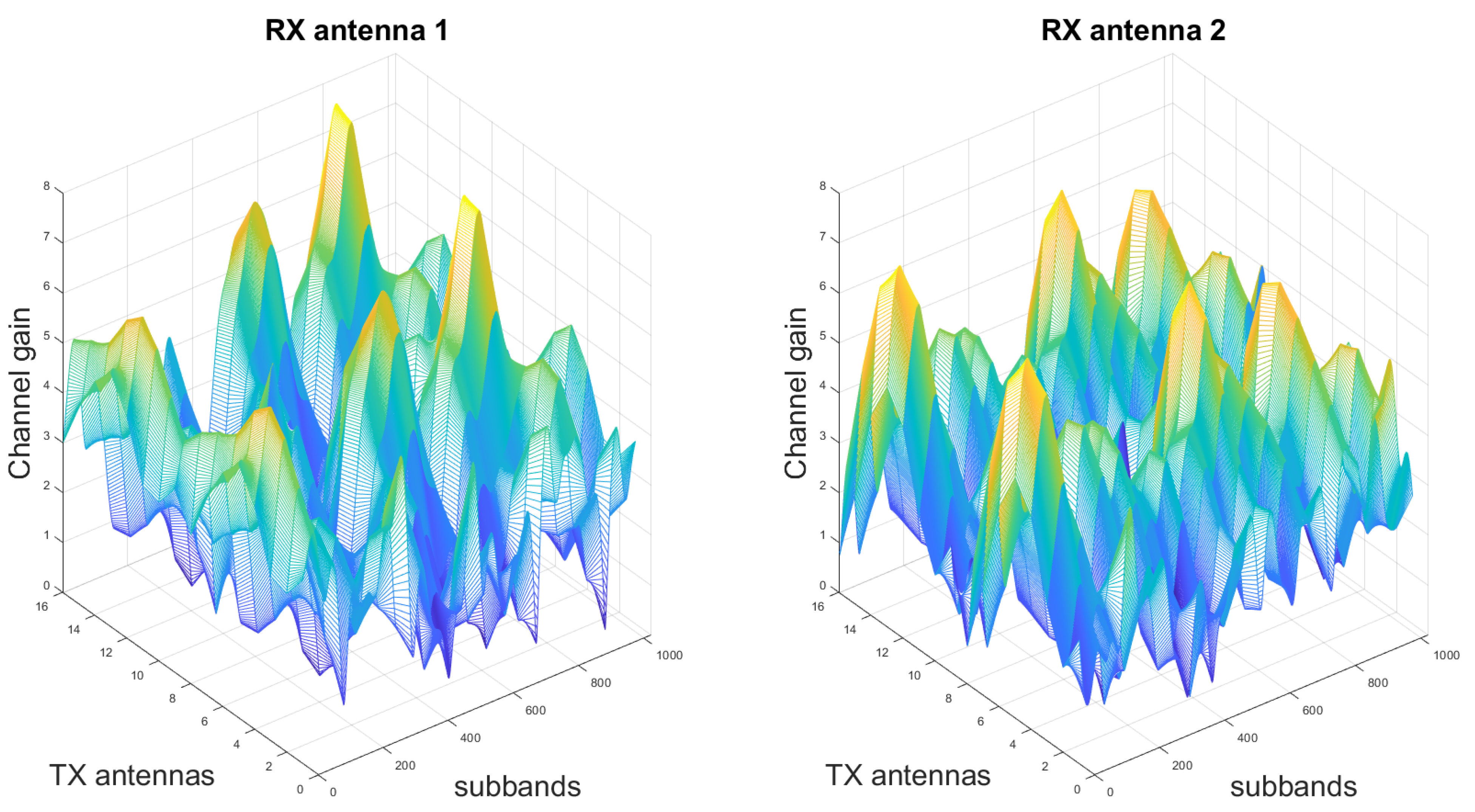
In this section, we report the results obtained by simulating the OFDM system and the channel generation previously described. The overall system parameters can be found in

Table 1. Simulation parameters.

Parameter	Value
Scenario	UMi
Radius of the cell R	100 m
Network loading or user density $\mu$	2500 users/km2
Carrier frequency $f_c$	28 GHz
Sampling frequency $f_s$	61.44 MSamples/s
OFDM Symbol time $T_{sym}$	16.67 $\mathsf{\mu }$s
Cyclic Prefix $T_{CP}$	$\frac{1}{16}\times T_{sym}$
Bandwidth B	50 MHz
Subcarrier spacing (SCS) $\Delta$	60 kHz
Active Subcarriers	792
$N_{FFT}$	1024
Noise figure F	7 dB
Maximum TX power $P_{tot}$	47 dBm
Total antennas per BS UPA $N_t$	72
Antennas along y for BS UPA $N_{ty}$	36, 24, 18
Antennas along z for BS UPA $N_{tz}$	2, 3, 4
Antennas along y for UT $N_{ry}$	1, 2
Antennas along z for UT $N_{rz}$	1
Polarizations	single, dual
Indoor UTs	80%

. Figure 7 reports an example of channel realization in the frequency domain, i.e., channel coefficient gains of the channel tensor ${\widetilde{\mathbf{\mathscr{H}}}}_{s,k}$ are shown after following all the steps described in Section 2 and Section 3 with $N_{FFT}=1024$ subcarriers, $N_t=16$ transmitting antennas at the BS ($N_{ty}=8$ and $N_{tz}=2$) and $N_r=N_{ry}=2$ receiving antennas, single polarized.

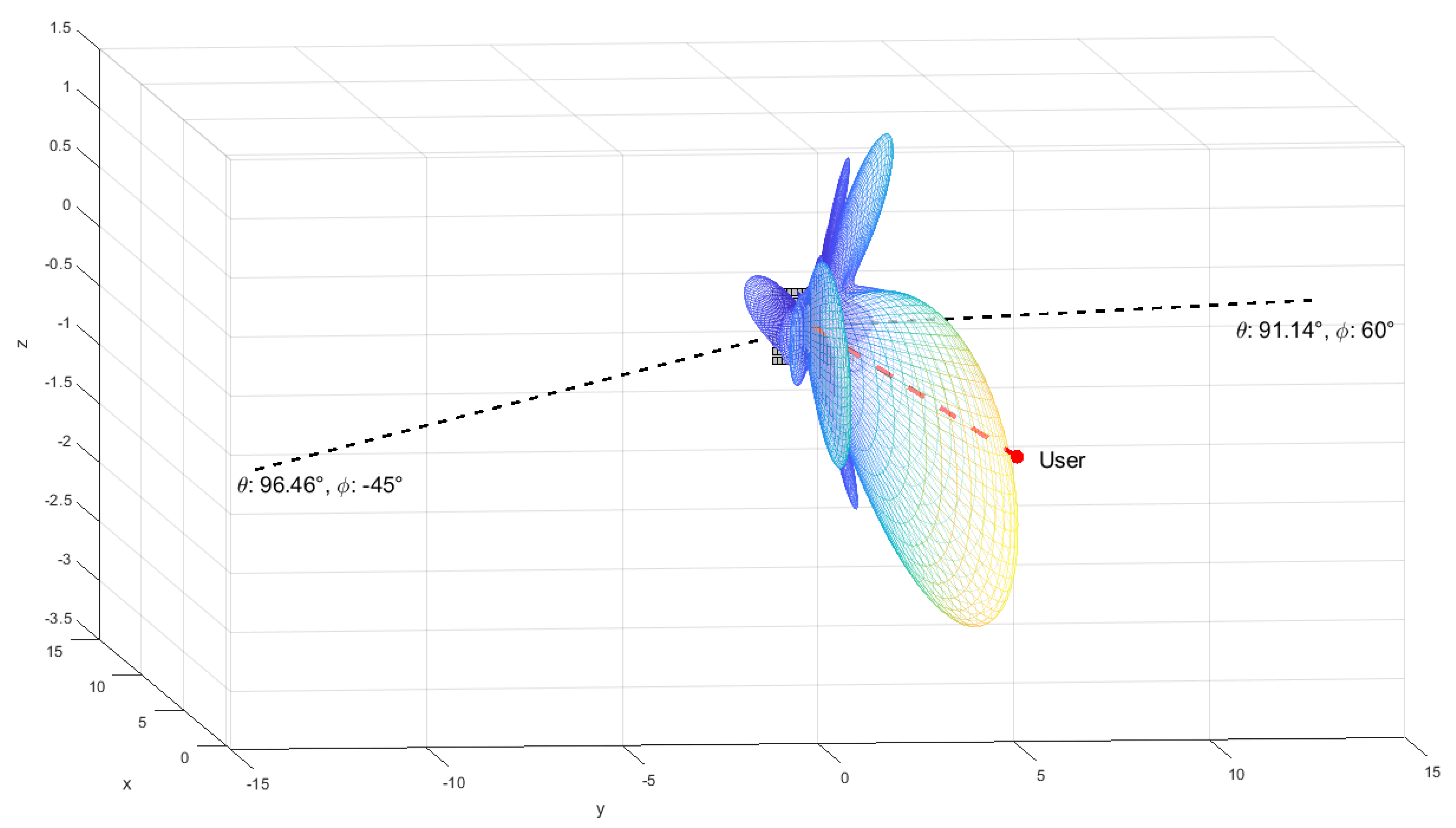
In particular, we identify some interesting scenarios to characterize our system, and then we collect results on its behavior when SLNR precoding is adopted as a precoding technique at BS and MMSE, combining at each UT when multi-layer features are enabled. The results are always reported as a Cumulative Distribution Function (CDF) curve of the achievable UT rates, except for the last scenario, where the total Sum-Rate is plotted against the traffic loading. When dual polarized elements are used, the total number of antenna elements becomes $2N_t$ at the transmitter and $2N_r$ at the receiver. As an example of SLNR precoding capabilities, Figure 8 shows the UPA radiation pattern at the BS when the SLNR precoding vector ${\mathbf{w}}_k$ targeted for user k (${\theta }_{LOS,ZOD}=96.{46}^{\circ }$, ${\varphi }_{LOS,AOD}={30}^{\circ }$) is implemented. In the depicted scenario with three total UTs with LOS condition, the precoder is able to minimize the interference that the user of interest may cause to the two other users, whose LOS direction of departures are shown.

5.1. Rates for Different UPA Configurations at the BS

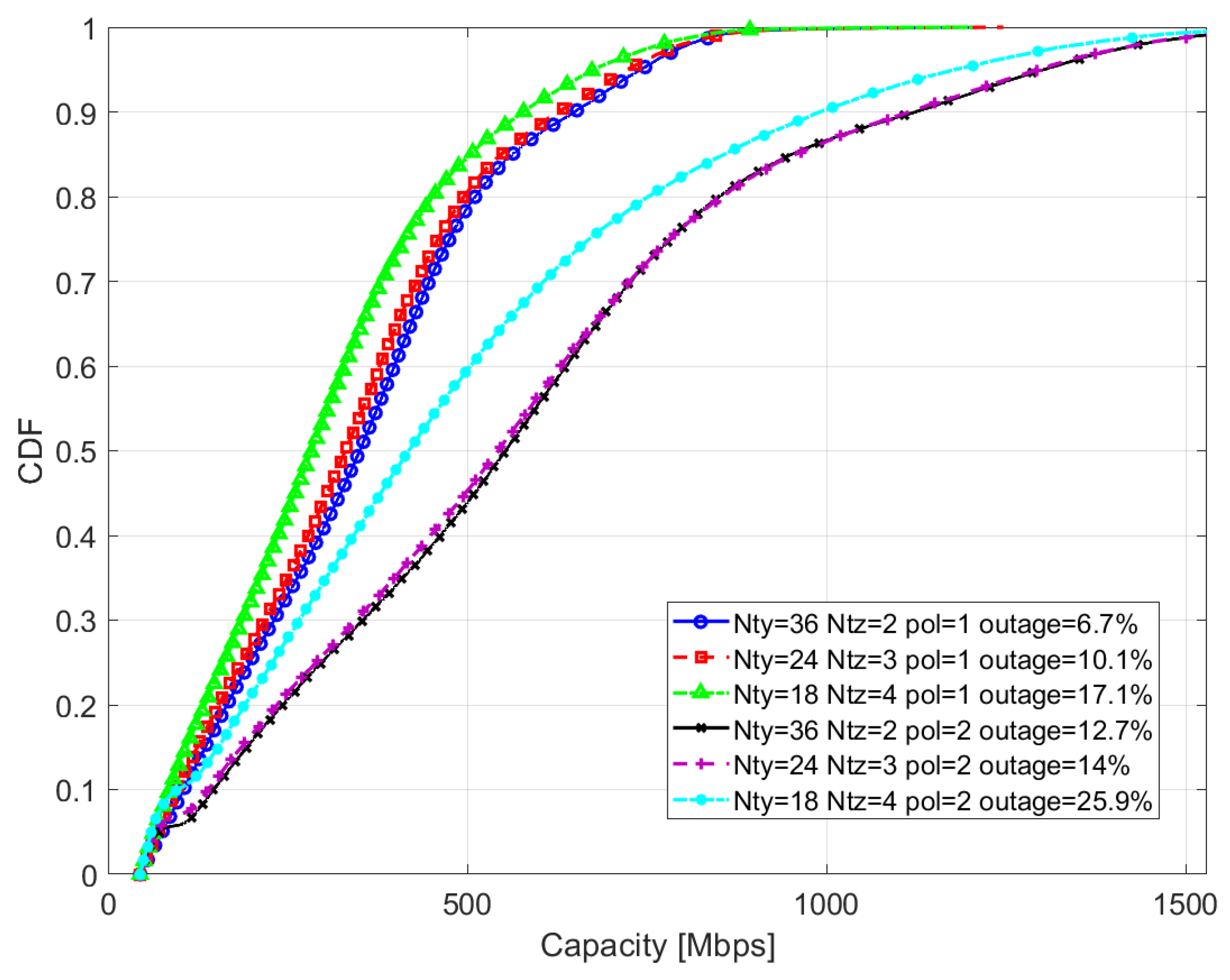
The multiplexing capabilities of the antenna array at the BS does not depend only on the number of antenna elements, but also on its geometrical configuration. In case of an UPA array, different configurations correspond to different number of columns and rows, changing respectively the number of elements along the y-axis $N_{ty}$ and along the z-axis $N_{tz}$. In order to evaluate the potential benefits of adopting one configuration rather than another, we simulate the same scenario with 72 antennas at the transmitter $N_t$, but spanning three possible antenna arrays configurations $N_{ty}\times N_{tz}$: $[36\times 2]$, $[24\times 3]$ and $[18\times 4]$. Moreover, the same configurations are compared both for the case of single and dual polarized elements. Given a traffic density of 2500 users/km${}^2$, we expect, on average, 65 UTs in the cell, equally divided among the three sectors. Of course, the rates could be significantly lower depending on the particular channel realizations and interference. A UT is in outage if its SINR is lower than 0 dB. The six CDF curves obtained in this test are displayed in Figure 9. In the case of dual polarized elements, whereas for $[36\times 2]$ and $[24\times 3]$ configurations the curves are very close, the curve for $[18\times 4]$ configuration is subject to a noticeable rate loss. For single polarized elements, the $[36\times 2]$ configuration performs better. This could be explained by the higher resolution required along the azimuth angle $\varphi$ rather than the zenith angle $\theta$, considering the possible user positions. However, each cell sector permits to serve the major percentage of the UTs simultaneously, achieving rates up to 800 Mbps for the single polarization and almost twice as much for the dual polarization.

5.2. Rates for Different Transmitting Powers

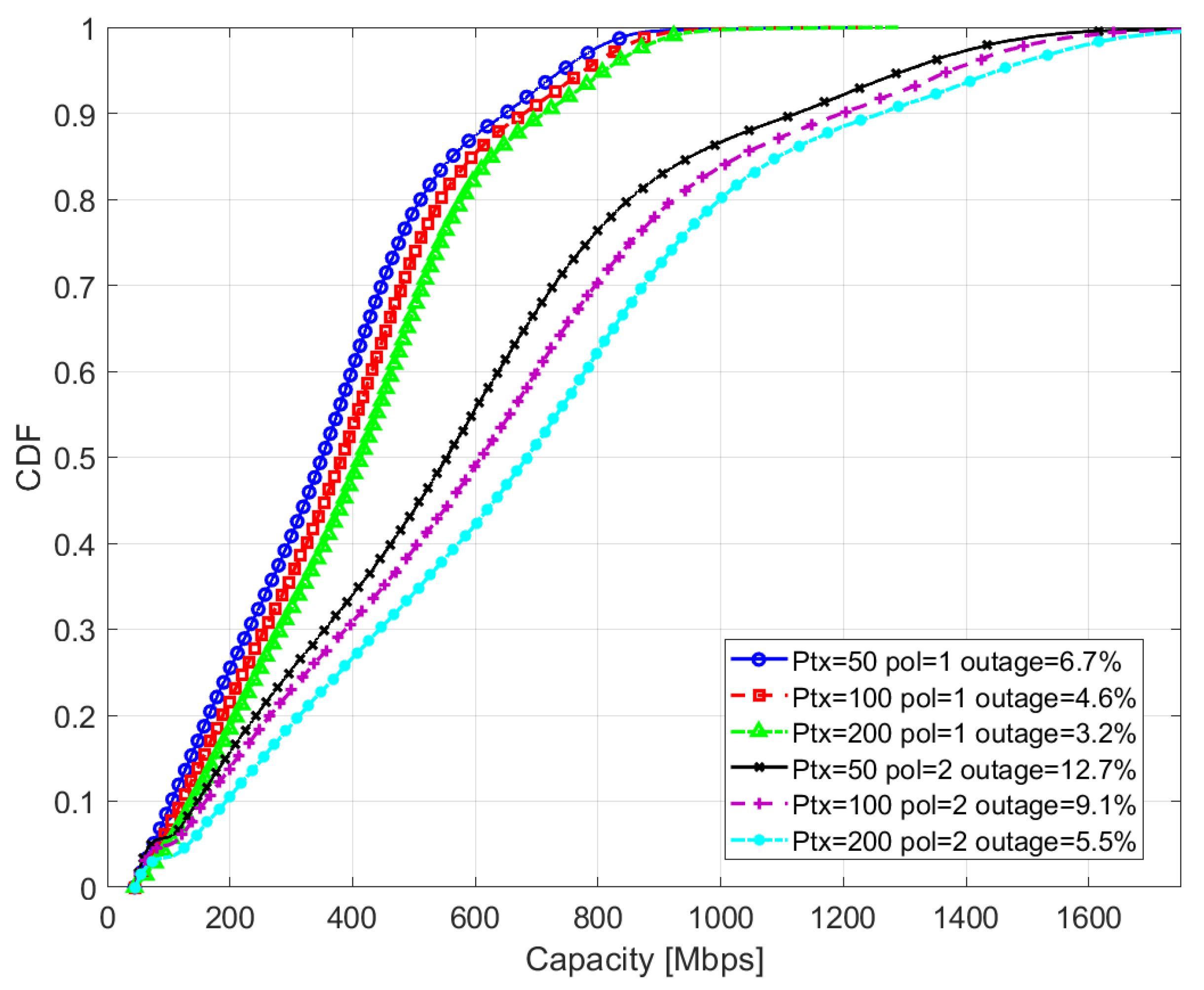
The power allocation is a critical design aspect in the deployment of a communication system. It can improve the SINR and so the capacity, but only with a logarithmic scaling. Thus, we test the performance of the system according to an increase on the transmitting power $P_{TX}$. The chosen values are 47 dBm (50 W), 50 dBm (100 W), and 53 dBm (200 W). The other parameters are the same as before, but now we adopt a fixed UPA configuration of $[36\times 2]$, in both the single and dual elements polarization case. Figure 10 shows the shift of the CDF curves towards higher rates together with the power increase, in both polarization options, and the outage tends to decrease. This is not a surprising result, as the SINR will benefit from a higher $P_{TX}$. Nevertheless, we should consider that a stronger signal could increase the interference among other cell sites in the nearby area.

5.3. Rates for Different Indoor Percentage

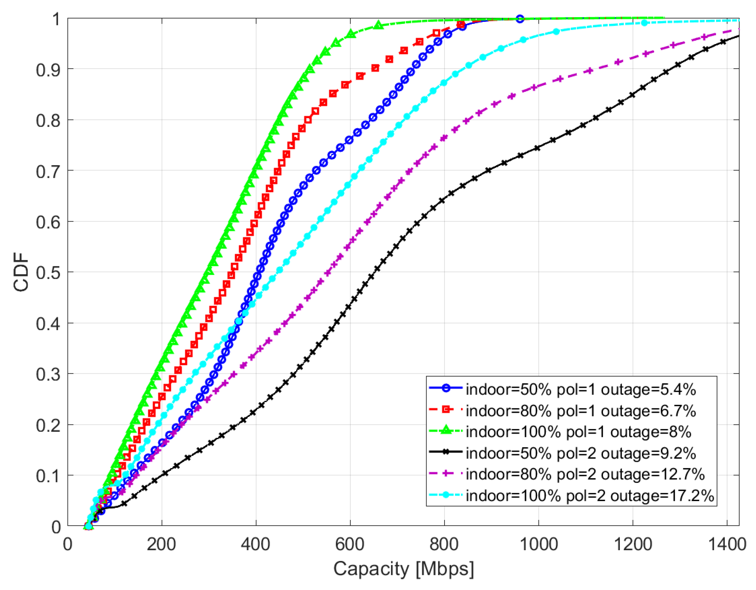
The parameter determining the percentage of users in an indoor condition could highly impact the rate of the users. This is of course caused by the higher losses encountered by the signal propagation and the absence of the LOS component whenever a certain UT is inside a building. This harmful effect is visible in Figure 11, where the CDF curves represent percentage of indoor UTs ranging from 0% to 100%. The number of UTs below the acceptable SINR threshold rises for higher indoor percentages. It is interesting to observe how two inflection points arise in the CDFs as the percentage of indoor users decreases. Additionally, in this case, the results for the two possible polarizations of the antenna elements show the same behavior.

5.4. Rates for Different Layers and Antenna Polarizations

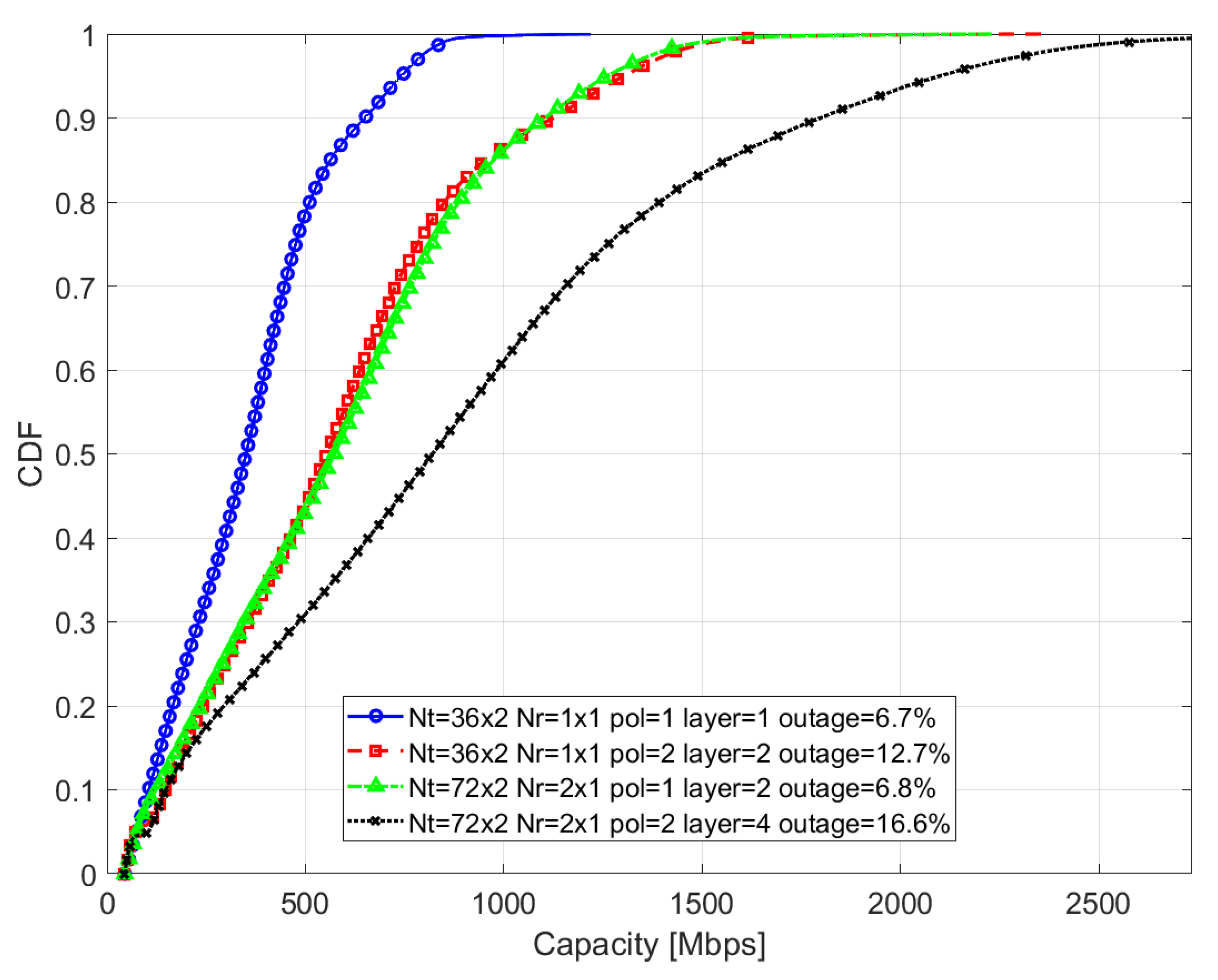
We studied the impact of layers and polarization on the per-user rate. Furthermore, we examine whether it is better for an array configuration to deploy dual cross polarized antenna elements, or to double the number of single polarized antenna elements at the BS and UTs. This comparison can be seen between $N_t=[36\times 2]$, $N_r=1$ dual polarized and $N_t=[72\times 2]$, $N_r=[2\times 1]$ single polarized elements configurations in Figure 12. For a given couple of $N_{ty}$ and $N_{tz}$, the antenna array with dual polarized elements improves the rate of the UTs, as the number of antenna elements are doubled. Nevertheless, in the case of equal number of elements, the configuration with single polarized elements exhibits a lower outage percentage, as the increase in the array dimension allows a better interference rejection capability.

5.5. Rates for Different Cell Radius Lengths

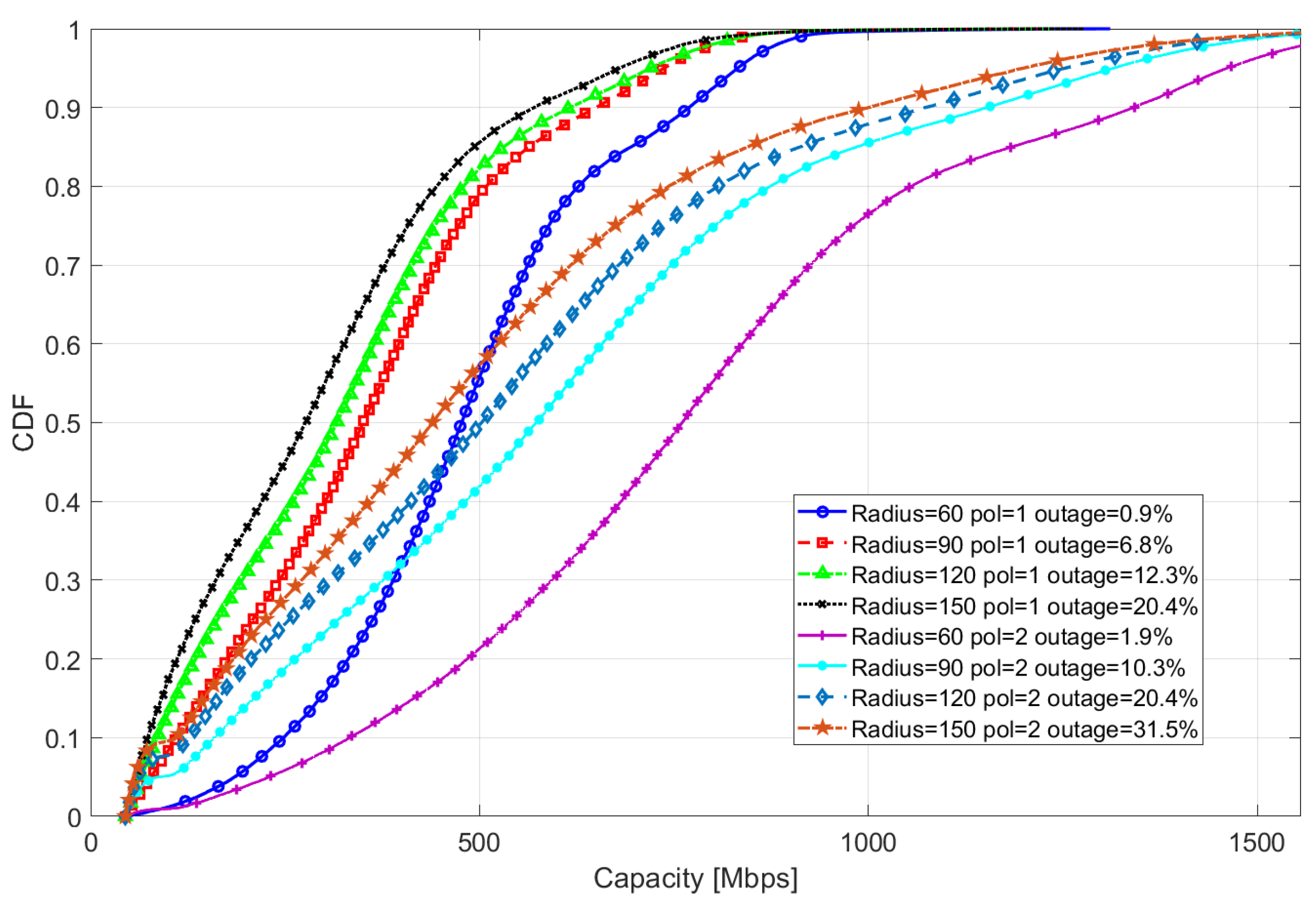
The last analyzed CDFs are generated with different cell sizes, i.e., different radius lengths. By taking into account the path loss term, it is easy to expect lower per-users SINRs, on average, as the cell radius increases; the greater the distance between BS and UT, the greater the path loss. This behavior is clearly represented in Figure 13. We considered a fixed average number of UTs inside the cell for all different cell sizes, therefore the users’ density $\mu$ is changed accordingly such that $\mu \frac{3\sqrt{3}}{2}{R}^2\approx$ 65. Both outage and rate show better results for smaller cell radius.

5.6. Sum Rate and Spectral Efficiency for Different Traffic Conditions

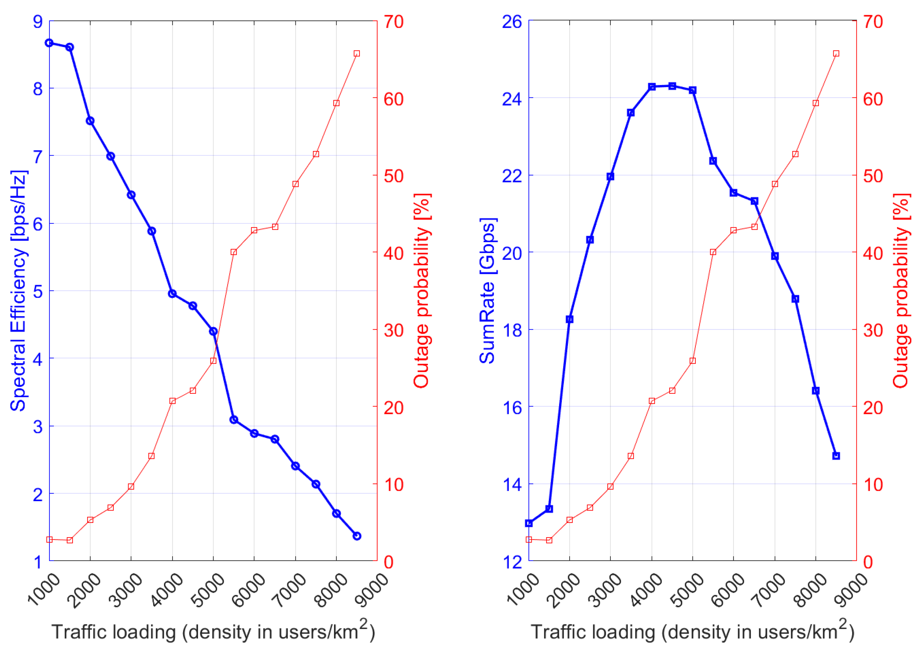
The SLNR precoding allows us to spatially multiplex users in an effective way. In Figure 14 we examine the interference rejection capability of the SLNR precoder by varying the traffic loading. In particular, we analyze the average spectral efficiency (averaged over all subcarriers for each user and over all users) and we detect the maximum attainable sum rate before experiencing a noticeable sum rate loss. At first, the total sum rate will likely increase as long as the number of users per sector does not significantly exceed the number of antennas $N_{ty}$ at the BS along the horizontal axis, even if the per-user spectral efficiency will decrease, as the power must be split among more transmissions. Nevertheless, when the density of the users in the sector becomes too high, the sum rate drops, then more and more users will experience outage as their SINR becomes too low to communicate with the BS. The peak of the sum rate roughly reaches 24 Gbps in the correspondence of traffic loading of approximately $\mu =4500$ users/km${}^2$, i.e., $\frac{1}{3}\mu \frac{3\sqrt{3}}{2}{R}^2\approx 39$. The curve of the spectral efficiency follows an almost linearly decreasing behavior w.r.t. the number of UTs. As expected, the outage probability is directly proportional to the traffic loading.

6. Conclusions

In this paper, we have presented the new 3-D channel model for 5G designed by 3GPP in TR 38.901, providing a step-by-step tutorial of its implementation in MATLAB. The new channel model characterizes the rich environment in which signal propagation takes place, with the customization of a significant number of parameters. This allows us to run extensive simulations to test new systems before their actual implementation. Furthermore, we have deomstrated an OFDM MIMO system by simulating a trisectorial single cell 5G cellular network. The developed system uniquely resorts on SDMA techniques, based on SLNR precoding and MMSE combining schemes, to establish communication between the BS and UTs, which are randomly generated and located in the cell. We have implemented our system with different configurations for antenna arrays on both the transmitter and receiver sides. We have shown that the number of the antenna elements and their arrangement can affect the efficiency of MIMO techniques, as well as the adoption of double cross-polarized antenna elements instead of single polarized ones. From the results obtained by a variety of simulations, we have investigated how the achievable rates and the outages of the users may change according to the chosen parameters, such as the array configuration, the number of layers and polarizations, the traffic density, the transmission power, the percentage of indoor UTs and the cell radius. SLNR precoding shows great performance in efficiently multiplexing different UTs in a cell sector, but it shows some limitations when the users are spatially correlated, as it might be expected. This behavior becomes more and more evident as the density of users increases. Future works will aim at broadening the current channel generation to support the mobility of the users, but also at studying efficient scheduling algorithms to better exploit the benefits of MU-MIMO techniques, i.e., by grouping or clustering users in order to limit their spatial correlation and, consequently, their interference.

References

Mort, G.S.; Drennan, J. Mobile communications: A study of factors influencing consumer use of m-services. J. Advert. Res.2007, 47, 302–312. [Google Scholar] [CrossRef] [Green Version]
Linke, C. Mobile media and communication in everyday life: Milestones and challenges. Mob. Media Commun.2013, 1, 32–37. [Google Scholar] [CrossRef]
Roh, W.; Seol, J.Y.; Park, J.; Lee, B.; Lee, J.; Kim, Y.; Cho, J.; Cheun, K.; Aryanfar, F. Millimeter-wave beamforming as an enabling technology for 5G cellular communications: Theoretical feasibility and prototype results. IEEE Commun. Mag.2014, 52, 106–113. [Google Scholar] [CrossRef]
Han, S.; Chih-Lin, I.; Xu, Z.; Rowell, C. Large-scale antenna systems with hybrid analog and digital beamforming for millimeter wave 5G. IEEE Commun. Mag.2015, 53, 186–194. [Google Scholar] [CrossRef]
Akdeniz, M.R.; Liu, Y.; Samimi, M.K.; Sun, S.; Rangan, S.; Rappaport, T.S.; Erkip, E. Millimeter Wave Channel Modeling and Cellular Capacity Evaluation. IEEE J. Sel. Areas Commun.2014, 32, 1164–1179. [Google Scholar] [CrossRef]
Shafi, M.; Zhang, M.; Moustakas, A.; Smith, P.; Molisch, A.; Tufvesson, F.; Simon, S. Polarized MIMO channels in 3-D: Models, measurements and mutual information. IEEE J. Sel. Areas Commun.2006, 24, 514–527. [Google Scholar] [CrossRef]
Ding, Z.; Lei, X.; Karagiannidis, G.K.; Schober, R.; Yuan, J.; Bhargava, V.K. A Survey on Non-Orthogonal Multiple Access for 5G Networks: Research Challenges and Future Trends. IEEE J. Sel. Areas Commun.2017, 35, 2181–2195. [Google Scholar] [CrossRef] [Green Version]
Mitola, J. Cognitive Radio Architecture Evolution. Proc. IEEE2009, 97, 626–641. [Google Scholar] [CrossRef]
Sasipriya, S.; Vigneshram, R. An overview of cognitive radio in 5G wireless communications. In Proceedings of the 2016 IEEE International Conference on Computational Intelligence and Computing Research (ICCIC), Chennai, India, 15–17 December 2016; pp. 1–5. [Google Scholar] [CrossRef]
Axell, E.; Leus, G.; Larsson, E.G.; Poor, H.V. Spectrum Sensing for Cognitive Radio: State-of-the-Art and Recent Advances. IEEE Signal Process. Mag.2012, 29, 101–116. [Google Scholar] [CrossRef] [Green Version]
Riviello, D.; Benco, S.; Crespi, F.L.; Ghittino, A.; Garello, R.; Perotti, A. Spectrum Sensing Algorithms for Cognitive TV White-Spaces Systems. In Cognitive Communication and Cooperative HetNet Coexistence: Selected Advances on Spectrum Sensing, Learning, and Security Approaches; Springer International Publishing: Cham, Switzerland, 2014; pp. 71–90. [Google Scholar] [CrossRef]
Bagwari, A.; Tuteja, S.; Bagwari, J.; Samarah, A. Spectrum Sensing Techniques for Cognitive Radio: A Re-examination. In Proceedings of the 2020 IEEE 9th International Conference on Communication Systems and Network Technologies (CSNT), Gwalior, India, 10–12 April 2020; pp. 93–96. [Google Scholar] [CrossRef]
Koyuncu, H.; Bagwari, A.; Tomar, G.S. Simulation of a Smart Sensor Detection Scheme for Wireless Communication Based on Modeling. Electronics2020, 9, 1506. [Google Scholar] [CrossRef]
Spencer, Q.; Swindlehurst, A.; Haardt, M. Zero-forcing methods for downlink spatial multiplexing in multiuser MIMO channels. IEEE Trans. Signal Process.2004, 52, 461–471. [Google Scholar] [CrossRef]
Joham, M.; Utschick, W.; Nossek, J. Linear transmit processing in MIMO communications systems. IEEE Trans. Signal Process.2005, 53, 2700–2712. [Google Scholar] [CrossRef]
Tarighat, A.; Sadek, M.; Sayed, A. A multi user beamforming scheme for downlink MIMO channels based on maximizing signal-to-leakage ratios. In Proceedings of the (ICASSP ’05)—IEEE International Conference on Acoustics, Speech, and Signal Processing, Philadelphia, PA, USA, 23–23 March 2005; Volume 3, pp. iii/1129–iii/1132. [Google Scholar] [CrossRef]
Sadek, M.; Aïssa, S. Leakage Based Precoding for Multi-User MIMO-OFDM Systems. IEEE Trans. Wirel. Commun.2011, 10, 2428–2433. [Google Scholar] [CrossRef]
Patcharamaneepakorn, P.; Armour, S.; Doufexi, A. On the Equivalence Between SLNR and MMSE Precoding Schemes with Single-Antenna Receivers. IEEE Commun. Lett.2012, 16, 1034–1037. [Google Scholar] [CrossRef] [Green Version]
Yang, C. An Enhanced Leakage-Based Precoding Scheme for Multi-User Multi-Layer MIMO Systems. arXiv2014, arXiv:1407.3866. [Google Scholar]
3GPP. Study on Channel Model for Frequencies from 0.5 to 100 GHz (Release 16) V16.1.0; Technical Report; Rep. TR 38.901; 3GPP: Sophia Antipolis, France, 2020. [Google Scholar]
Osseiran, A.; Boccardi, F.; Braun, V.; Kusume, K.; Marsch, P.; Maternia, M.; Queseth, O.; Schellmann, M.; Schotten, H.; Taoka, H.; et al. Scenarios for 5G mobile and wireless communications: The vision of the METIS project. IEEE Commun. Mag.2014, 52, 26–35. [Google Scholar] [CrossRef]
Kyösti, P.; Meinilä, J.; Hentilä, L.; Zhao, X.; Jämsä, T.; Schneider, C.; Narandžić, M.; Milojević, M.; Hong, A.; Ylitalo, J.; et al. WINNER II Channel Models, WINNER II D1. 1.2, v1. 2. WINNER, Rep. IST-4-027756. 2008. Available online: http://www.ero.dk/93F2FC5C-0C4B-4E44-8931-00A5B05A331B (accessed on 15 December 2021).
Jaeckel, S.; Raschkowski, L.; Börner, K.; Thiele, L. QuaDRiGa: A 3-D Multi-Cell Channel Model With Time Evolution for Enabling Virtual Field Trials. IEEE Trans. Antennas Propag.2014, 62, 3242–3256. [Google Scholar] [CrossRef]
Bian, J.; Sun, J.; Wang, C.X.; Feng, R.; Huang, J.; Yang, Y.; Zhang, M. A WINNER+ based 3-D non-stationary wideband MIMO channel model. IEEE Trans. Wirel. Commun.2017, 17, 1755–1767. [Google Scholar] [CrossRef]
Xiao, H.; Burr, A.G.; Song, L. A time-variant wideband spatial channel model based on the 3GPP model. In Proceedings of the IEEE Vehicular Technology Conference, Melbourne, Australia, 25–28 September 2006; pp. 1–5. [Google Scholar]
Baum, D.S.; Hansen, J.; Salo, J.; Del Galdo, G.; Milojevic, M.; Kyösti, P. An interim channel model for beyond-3G systems: Extending the 3GPP spatial channel model (SCM). In Proceedings of the 2005 IEEE 61st Vehicular Technology Conference, Stockholm, Sweden, 30 April–1 May 2005; Volume 5, pp. 3132–3136. [Google Scholar]
QuaDRiGa. Quadriga: The Next Generation Radio Channel Model. 2014. Available online: https://quadriga-channel-model.de/ (accessed on 15 December 2021).
Peter, M.; Haneda, K.; Nguyen, S.; Karttunen, A.; Järveläinen, J. Measurement results and final mmMAGIC channel models. Deliv. D22017, 2, 12. [Google Scholar]
Nurmela, V.; Karttunen, A.; Roivainen, A.; Raschkowski, L.; Hovinen, V.; Eb, J.Y.; Omaki, N.; Kusume, K.; Hekkala, A.; Weiler, R.; et al. METIS Channel Models. Deliverable D1.4. 2015. Available online: https://metis2020.com/wp-content/uploads/deliverables/METIS_D1.4_v1.0.pdf (accessed on 15 December 2021).
Jämsä, T.; Kyösti, P. Device-to-device extension to geometry-based stochastic channel models. In Proceedings of the IEEE 2015 9th European Conference on Antennas and Propagation (EuCAP), Lisbon, Portugal, 13–17 April 2015; pp. 1–4. [Google Scholar]
Wang, Z.; Tameh, E.; Nix, A. A sum-of-sinusoids based simulation model for the joint shadowing process in urban peer-to-peer radio channels. In Proceedings of the VTC-2005-Fall, 2005 IEEE 62nd Vehicular Technology Conference, Dallas, TX, USA, 28 September 2005; Volume 3, pp. 1732–1736. [Google Scholar] [CrossRef] [Green Version]
Zhao, X.; Du, F.; Geng, S.; Sun, N.; Zhang, Y.; Fu, Z.; Wang, G. Neural network and GBSM based time-varying and stochastic channel modeling for 5G millimeter wave communications. China Commun.2019, 16, 80–90. [Google Scholar] [CrossRef]
Samimi, M.K.; Rappaport, T.S. 3-D statistical channel model for millimeter-wave outdoor mobile broadband communications. In Proceedings of the 2015 IEEE International Conference on Communications (ICC), London, UK, 8–12 June 2015; pp. 2430–2436. [Google Scholar]
Samimi, M.K.; Rappaport, T.S. 3-D millimeter-wave statistical channel model for 5G wireless system design. IEEE Trans. Microw. Theory Tech.2016, 64, 2207–2225. [Google Scholar] [CrossRef]
Samimi, M.K.; Rappaport, T.S. Statistical channel model with multi-frequency and arbitrary antenna beamwidth for millimeter-wave outdoor communications. In Proceedings of the 2015 IEEE Globecom Workshops (GC Wkshps), San Diego, CA, USA, 6–10 December 2015; pp. 1–7. [Google Scholar]
Rappaport, T.S.; Sun, S.; Mayzus, R.; Zhao, H.; Azar, Y.; Wang, K.; Wong, G.N.; Schulz, J.K.; Samimi, M.; Gutierrez, F. Millimeter wave mobile communications for 5G cellular: It will work! IEEE Access2013, 1, 335–349. [Google Scholar] [CrossRef]
Kim, N.; Lee, Y.; Park, H. Performance Analysis of MIMO System with Linear MMSE Receiver. IEEE Trans. Wirel. Commun.2008, 7, 4474–4478. [Google Scholar] [CrossRef]
Sadek, M.; Tarighat, A.; Sayed, A.H. Active Antenna Selection in Multiuser MIMO Communications. IEEE Trans. Signal Process.2007, 55, 1498–1510. [Google Scholar] [CrossRef]
Figure 1.
Hexagonal cell site divided into three sectors.
Figure 2.
Uniform Planar Array with cross-polarized antenna elements. .
Figure 3.
3GPP antenna element radiation pattern.
Figure 4.
Representation of the main clusters angles for a UT–BS link w.r.t. their powers and directions, in case of LOS.
Figure 5.
Multi-User Multi-Layer MIMO scheme.
Figure 6.
Cell site with 30 users after sector assignment. 3-D view on the left, 2-D top-view on the right.
Figure 7.
Channel frequency response along 1024 subbands, with 16 transmit antennas at the BS. , , . Single polarized.
Figure 8.
UPA radiation pattern with SLNR precoder targeted for UT k (, ) with two interfering users, , , for all users.
Figure 9.
CDF of UT rates for different UPA configurations at the TX, , , dBm, traffic density = 2500 users/km.
Figure 10.
CDF of UT rates for different transmitting powers at the BS, with , , , traffic density = 2500 users/km.
Figure 11.
CDF of UT rates for different user indoor percentages, with , , , dBm, traffic density = 2500 users/km.
Figure 12.
CDF of UT rates for different layers with single or dual polarized antenna elements, = , = , = 47 dBm, traffic density = 2500 users/km.
Figure 13.
CDF of UT rates for different cell radius lengths, with , , , dBm, average number of UTs in the cell, 65.
Figure 14.
Sum rate and average spectral efficiency of the UTs for different traffic density, with , , , single polarization, dBm.