
MaWGAN: A Generative Adversarial Network to Create Synthetic Data from Datasets with Missing Data


1
School of Mathematics, Cardiff University, Cardiff CF24 4AG, UK
2
School of Computer Science and Informatics, Cardiff University, Cardiff CF24 4AG, UK
*
Author to whom correspondence should be addressed.
Electronics 2022, 11(6), 837; https://0-doi-org.brum.beds.ac.uk/10.3390/electronics11060837
Submission received: 31 January 2022
/
Revised: 24 February 2022
/
Accepted: 4 March 2022
/
Published: 8 March 2022
(This article belongs to the Special Issue Recent Advances in Synthetic Data Generation)
Abstract
:The creation of synthetic data are important for a range of applications, for example, to anonymise sensitive datasets or to increase the volume of data in a dataset. When the target dataset has missing data, then it is common to just discard incomplete observations, even though this necessarily means some loss of information. However, when the proportion of missing data are large, discarding incomplete observations may not leave enough data to accurately estimate their joint distribution. Thus, there is a need for data synthesis methods capable of using datasets with missing data, to improve accuracy and, in more extreme cases, to make data synthesis possible. To achieve this, we propose a novel generative adversarial network (GAN) called MaWGAN (for masked Wasserstein GAN), which creates synthetic data directly from datasets with missing values. As with existing GAN approaches, the MaWGAN synthetic data generator generates samples from the full joint distribution. We introduce a novel methodology for comparing the generator output with the original data that does not require us to discard incomplete observations, based on a modification of the Wasserstein distance and easily implemented using masks generated from the pattern of missing data in the original dataset. Numerical experiments are used to demonstrate the superior performance of MaWGAN compared to (a) discarding incomplete observations before using a GAN, and (b) imputing missing values (using the GAIN algorithm) before using a GAN.
1. Introduction
Missing data is a common problem and can arise due to a variety of reasons. Rubin [1] defines three types of missing data: missing completely at random (MCAR), missing at random (MAR), and not missing at random (NMAR). Suppose that we have independent observations and put if is missing and 1 if it is present (we call the mask corresponding to ). The data are MCAR if for any j, is independent of , it is MAR if is independent of but dependent on some for , and NMAR if it is dependent on . We will assume that our dataset is MCAR.
A range of imputation methods exist to fill in missing values. Suppose that (so variable j is missing from observation i), different methods for imputing include
- Using the mean of the non-missing , [2].
- Using a (parametric) regression model for given , , built using complete observations. If the regression model includes a distribution for the error term, then we can use it to randomly impute (see stochastic regression imputation [5]).
- Using a (non-parametric) estimate of the conditional distribution of given , , to sample from. The GAIN methodology (generative adversarial imputation nets [6]) is an example of this approach using a GAN architecture.
An advantage of random imputation methods is that they allow the subsequent application of multivariate imputation methods such as MICE [7]. Table 1 lists the techniques mentioned above with a qualitative assessment of their relative accuracy and computational cost.
While there have been recent advances in synthetic data generation due to the application of machine-learning models, missing data have not received much attention. Synthetic data generation is increasingly important in a range of applications, for example, to increase dataset volume or to anonymise sensitive datasets [8,9], and in practice often has to deal with missing data. A promising development for data synthesis has been the advent of generative adversarial networks (GANs) [10]. GANs use two neural nets, one to generate synthetic data, and the other to build a critic, which is used to train the generator (also called a discriminator). The generator and critic are trained iteratively, so that as the generator improves the critic becomes more discerning, allowing further refinement of the generator. Until now, missing data have been a problem for GANs as existing algorithms require complete observations, so users have to either first impute the missing data or just discard incomplete observations. In this paper, we propose a novel GAN algorithm that can directly train a synthetic data generator from datasets with missing values; to our knowledge this is the first such attempt. We called it MaWGAN (for Masked Wasserstein GAN). As with existing GAN approaches, the MaWGAN synthetic data generator generates samples from the full joint distribution. The novelty of our approach is a methodology for comparing the generator output with the original data that does not require us to discard incomplete observations, based on a modification of the Wasserstein distance. Moreover, our approach is easily implemented by incorporating into the critic masks generated from the pattern of missing data in the original dataset.
2. Theoretical Basis
MaWGAN builds on the WGAN-GP algorithm [11,12]. Let be an i.i.d. sample from some (unknown) distribution , and let be our generator. G takes a vector of i.i.d. random variates and returns a vector with distribution say. The WGAN-GP critic calculates an estimate of the Wasserstein distance, so that the generator is trained to minimise the distance between and as measured by the Wasserstein distance.
Let be the set of measures on with marginals and , then the Wasserstein distance is
where is the Lipschitz constant of f. Let be our critic. Let be a sample from the generator G, and for put , then we train the critic to maximise
The key idea here is that the regularisation term will restrict the critic C to be close to a Lipschitz function with Lipschitz constant 1. Here, controls the degree of regularisation and can be tuned to improve the convergence of the critic.
We introduce a variation of the Wasserstein distance that incorporates a random mask to capture the effect of MCAR missing data. For our purposes a mask is an element of and a random mask is just a measure on . Given a data point and a mask , is treated as missing if and only if . We define the -Wasserstein distance as
where ⊙ represents pointwise multiplication. The following lemma shows that is equivalent to W in the topological sense (meaning they generate the same topology on the space of measures on ). The practical consequence of the lemma is that a sequence of measures (representing a sequence of improving generators) will converge to w.r.t. the Wasserstein distance if and only if they converge to w.r.t. the -Wasserstein distance.
Lemma 1.
Let be a random mask, then provided , there exists a constant , such that
Proof.
Upper bound. For any and we have , so
and, thus, integrating M w.r.t. , we get
Here, the second line follows because we can view as a realisation of projected onto the subspace corresponding to the non-zero co-ordinates of M, and similarly for .
Lower bound. For any function f, we have
whence . □
We approximate the -Wasserstein distance analogously to the WGAN-GP approach (1). Let be the mask corresponding to data point , then using our previous notation, we train the critic to maximise
Here, we interpret as replacing the missing values in with zeros, and replaces the corresponding values of with zeros.
3. Implementation
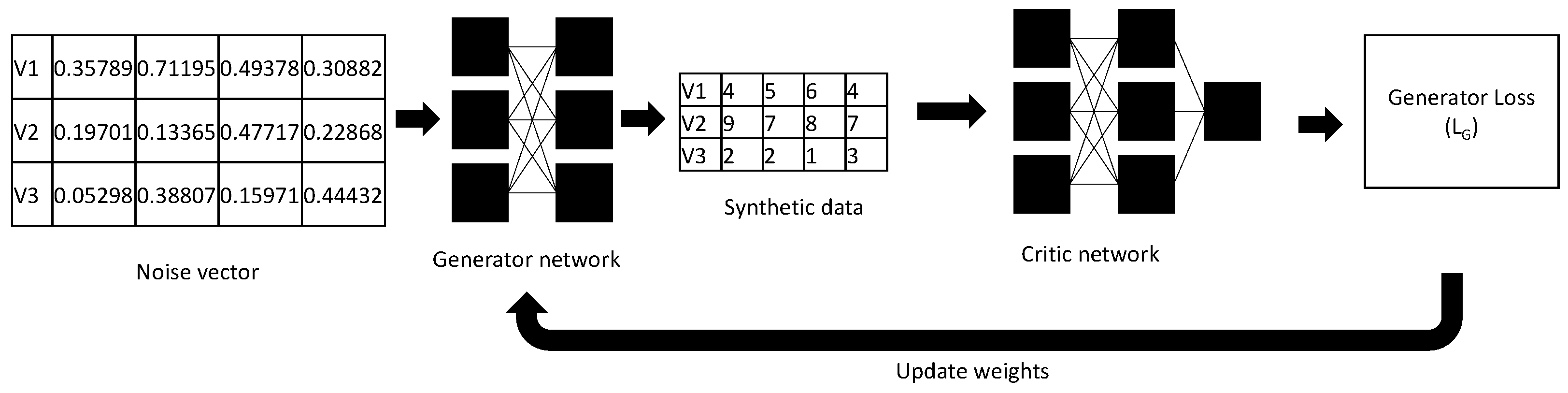
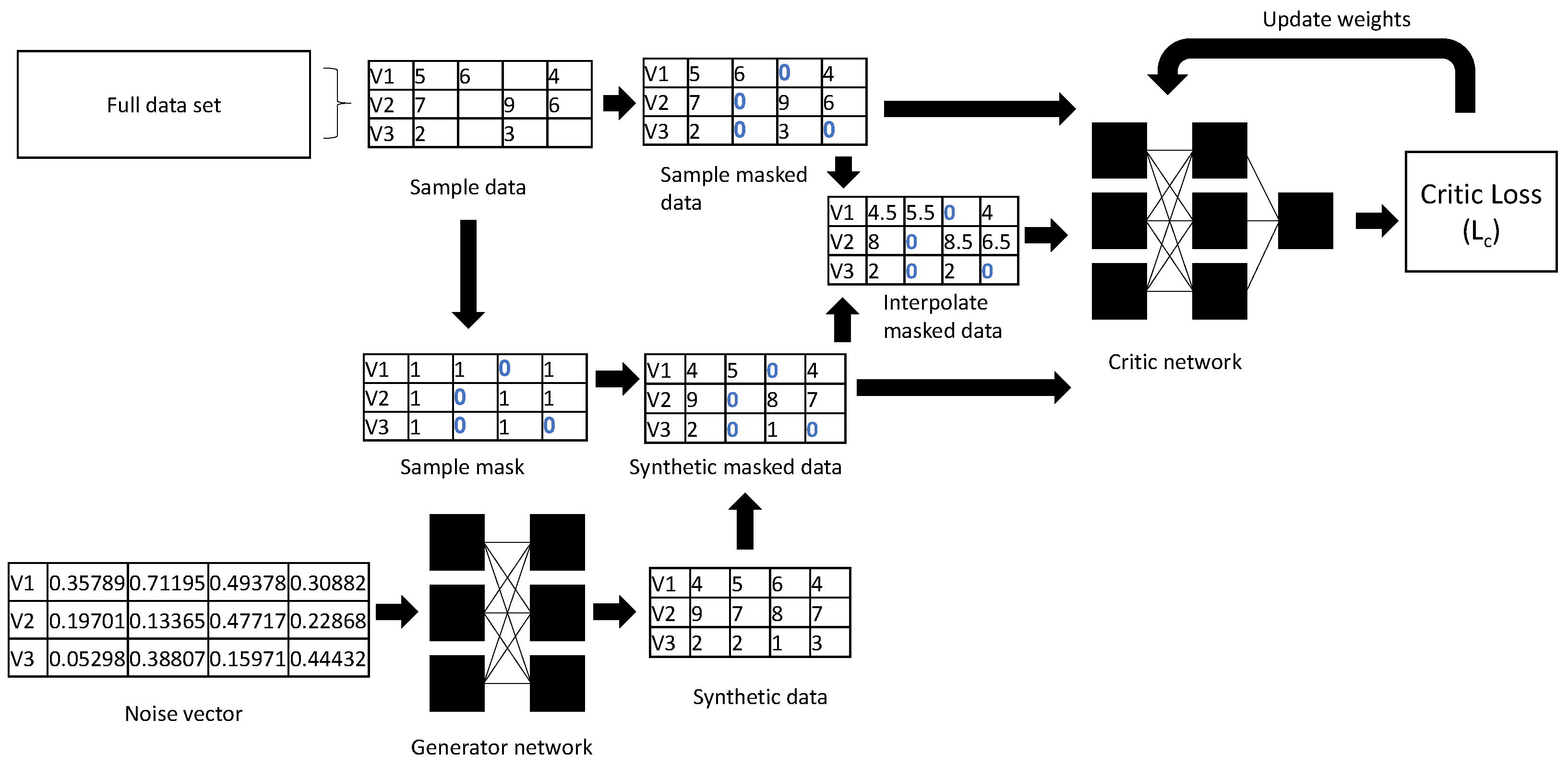
In this section, we explain the details of our MaWGAN implementation. Figure 1 and Figure 2 illustrate the flow of information in a single training step for the generator and critic respectively. In both cases, we calculate a loss that measures the performance of the generator/critic. Given the loss we calculate its gradient w.r.t. the weights (parameters) of the generator/critic, then update the weights in the direction of the gradient. Note that the generator is minimising its loss, so takes steps in the direction of the negative gradient, while the critic is maximising its loss, so take steps in the direction of the gradient.
Given the current critic, updating the generator is straightforward. We feed an array of random numbers into the generator one row at a time, to obtain an array of synthetic data (each row represents an independent realisation). We then feed the synthetic data into the critic, one row at a time, to obtain a vector of performance evaluations, which we average to obtain our loss.
To train the critic we need two sets of inputs: a sample (or batch) from the original dataset and a synthetic dataset of the same size produced by the generator. From the original dataset, we generate a mask indicating which data are missing, which we use to both replace the missing data with zeros, and replace the corresponding entries in the synthetic data array with zeros. We also generate an interpolated data array, which is just a linear combination of the masked original and masked synthetic data. The relative weights given to the original and synthetic data are chosen independently for each row. Each row of the original and synthetic data are fed into the critic, each row of the interpolated data array is fed into the gradient of the critic, and these are averaged as per Equation (2) to give the loss.
The pseudocode (Algorithm 1) shows how the generator and critic steps are interwoven. Note that for each update step of the gradient, we perform several updates of the critic, as we wish to keep the critic as a good approximation of the -Wasserstein distance.
| Algorithm 1 MaWGAN |
|
We have observations for , which we collect into an matrix X, where the i-th row of X is . Let be the mask corresponding to and let M be the matrix whose i-th row is . is our generator and our critic. Write for the weights that parameterise the generator G, and for the critic weights. It is and that we update when training G and C. The update steps require a learning rate , which we don’t explicitly include in our pseudocode.
In our algorithm we update the generator times, which we call epochs. For each epoch, the critic is updated times, and we use a batch of data size k. We will write for the batch and for its i-th element. is the regularisation parameter for the critic loss, which also needs to be set before hand.
4. Numerical Testing
Datasets. To test the performance of MaWGAN, we used three datasets of varying sizes and complexities. The Iris and Letter datasets are well known and can be found, for example, in the UCI Machine Learning Repository [13]. The Welsh Index of Multiple Deprivation is less well known, but was used because it has a flavour of the sort of official data that users want to synthesise for data-privacy reasons:
- The Welsh Index of Multiple Deprivation (WIMD) is the Welsh Government’s official measure of relative deprivation in Wales (UK); we used the 2014 figures [16]. For 1904 separate regions, the WIMD has measures of income, employment, education, and health. One region had a missing value and was removed from the dataset, leaving 1903 observations of 11 numerical variables.
- The Letter dataset was generated by Frey and Slate [17] and records 16 measured characteristics of images of the capital letters in the English alphabet. Letters were selected from 20 different fonts and randomly distorted a number of times; there were 20,000 observations of 16 numerical variables.
Simulated MCAR datasets. We generated eight additional versions of each dataset with 10%, 20%, …, 90% missing data. Points were removed at random with equal probability until the required percentage was reached. The additional datasets are nested in the sense that if an element is missing from one then it is missing from all versions with higher levels of missing data. By artificially removing data, we are able to compare the performance of our synthetic data generator with the complete dataset, even when it is trained with missing data.
Competing methodologies. MaWGAN was compared to two other approaches. The first is a two-step process where we apply the GAIN imputation method and then use WGAN-GP to train a generator on the completed data. The second alternative was to discard incomplete observations then use a WGAN-GP to train a generator on what remained. The number of remaining observations at the different levels of missingness are given in Table 2.
Performance metrics. To assess the performance of the three methods, we used two metrics, the Fréchet distance F and the likeness score L introduced by Guan and Loew [18]. To evaluate the performance of a data synthesis method, we need a metric that compares the distributions of the real and synthetic data, rather than single observations. There is no single best way of doing this and a number of approaches have been suggested in the literature (see for example the reviews of Borji [19,20]). Most of these are tailored to image data; however, the two we chose are very general in application. We found that metrics for comparing distributions need a lot of data to give really consistent results, though the likeness score has proved better in this regard than the others we have looked at.
Suppose we have observations from some distribution and observations from a second distribution, then to calculate L, we first generate three auxiliary sets of information
For let be the Kolmogorov–Smirnov distance between A and B, namely the maximum absolute difference between the empirical cumulative distribution functions of A and B. The likeness score for our two sets of observations is then
Note that and the two sets of observations have likeness one if and only if they are identical, with lower scores indicating greater dissimilarity.
The Fréchet distance F is given by
where and are the sample mean and sample covariance matrix of , and similarly for and . Smaller values indicate greater similarity, with if and only if the means and covariances are the same (which does not imply the samples are identical). It is common to calculate F not using the and directly but instead by first applying a feature extracting transform; in particular if the inception network is used then the resulting metric is called the Fréchet inception distance [21]. We do not do this in our case.
In our application the will always be one of the original three datasets, and the will be synthetic data generated by one of our three methods—subject to varying degrees of missing data—with . To reduce the variation due to sampling from the generator, we calculate F and L 100 times using different sets of synthetic data, then take the average for each.
4.1. Algorithmic Details
The MaWGAN, GAIN, and WGAN-GP algorithms were implemented in Python using the PyTorch library [22]. The MaWGAN and WGAN-GP implementations incorporated code publicly available on GitHub [23], and the GAIN implementation used the code provided by the original authors [6]. For both MaWGAN and WGAN-GP, the neural network architecture of both the generator and critic had five layers. For the generators, the input and output layers had nodes equal to the number of variables, and we used 150 nodes per hidden layer. For the critic, the input layer had nodes equal to the number of variables, output layer size 1, and we used 150 nodes per hidden layer. For training, we used = 15,000 epochs with training steps for the critic each time. We used a batch size of , a learning rate of , and critic regularisation .
An important practical observation is that when training a MaWGAN, the optimal tuning depends on the level of missing data. We found that as the level of missing data increases, the number of training steps for the critic in each epoch needs to increase ( in the pseudo-code above). Formally, considering (the component of the critic loss corresponding to observation i), we see that the variables that are masked do not contribute to the gradient of w.r.t. the critic weights . That is, the masking means that when updating , observation i only contributes information about the distribution of its non-missing variables. Thus, as is intuitively clear, the level of information available in each observation reduces as the level of missingness increases, and so we need to do more work to train the critic. If the critic does not get sufficient training in each epoch then the generator can converge too quickly to a lower-dimensional projection of the target distribution (so-called mode collapse).
4.2. Results
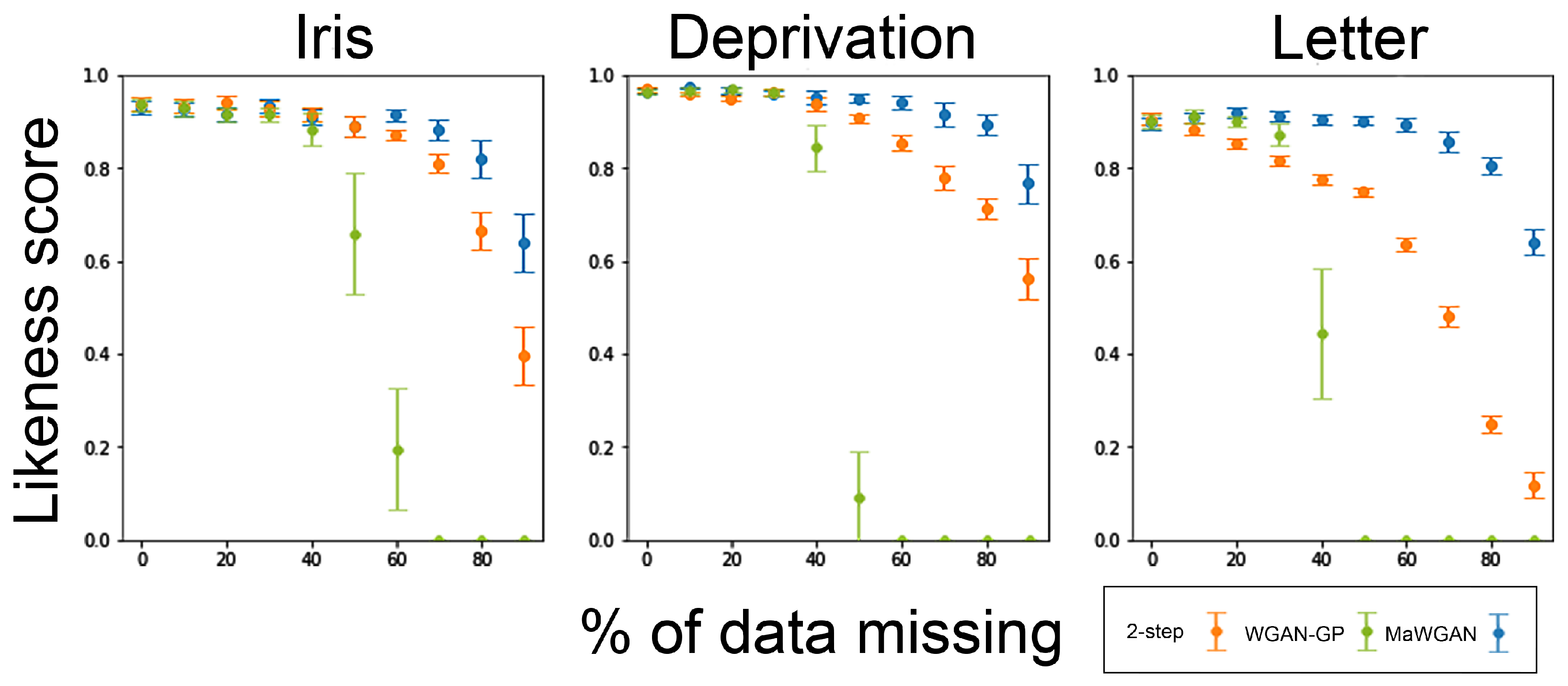
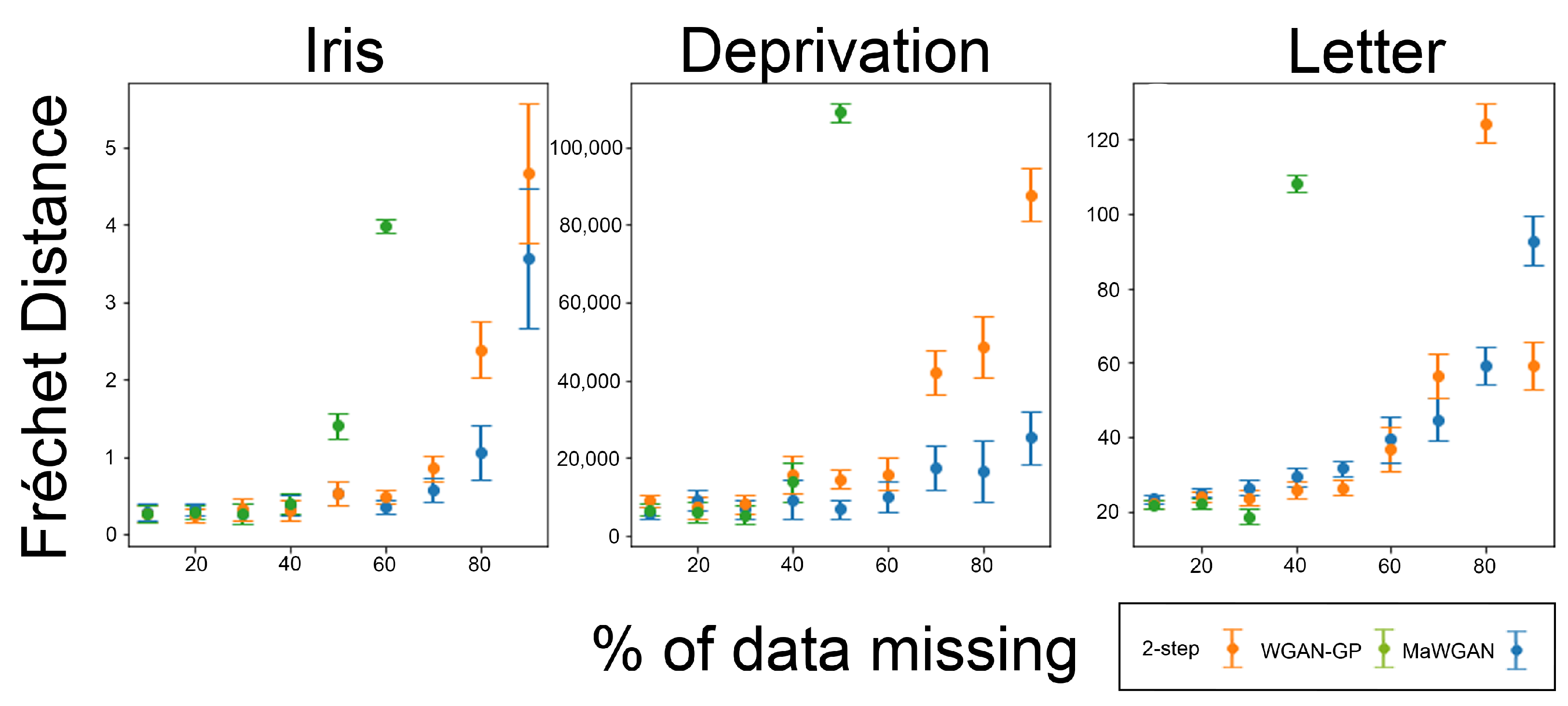
Because GAN training is stochastic, the performance of the resulting generator can vary. Accordingly for each combination of method, dataset and missingness we fitted the generator 20 times, calculating the likeness score and the Fréchet distance each time. The results are summarised in Figure 3 and Figure 4. For each combination of method, dataset, and missingness, we give the average performance and a 95% confidence interval for the mean.
Looking at the likeness score, the results show that for these datasets MaWGAN performs consistently well with levels of missing data up to 50%. MaWGAN also performs significantly better than both the two-step method and the complete observations method with moderate to high levels of missing data, and never performed any worse than either alternative.
With respect to the Fréchet distance, the picture is not as one-sided, though overall, MaWGAN still performs best. All three methods give similar levels of performance with up to 30% missing data. For higher levels of missing data the complete observations method is poor, while MaWGAN usually outperforms the two-step method, but not always.
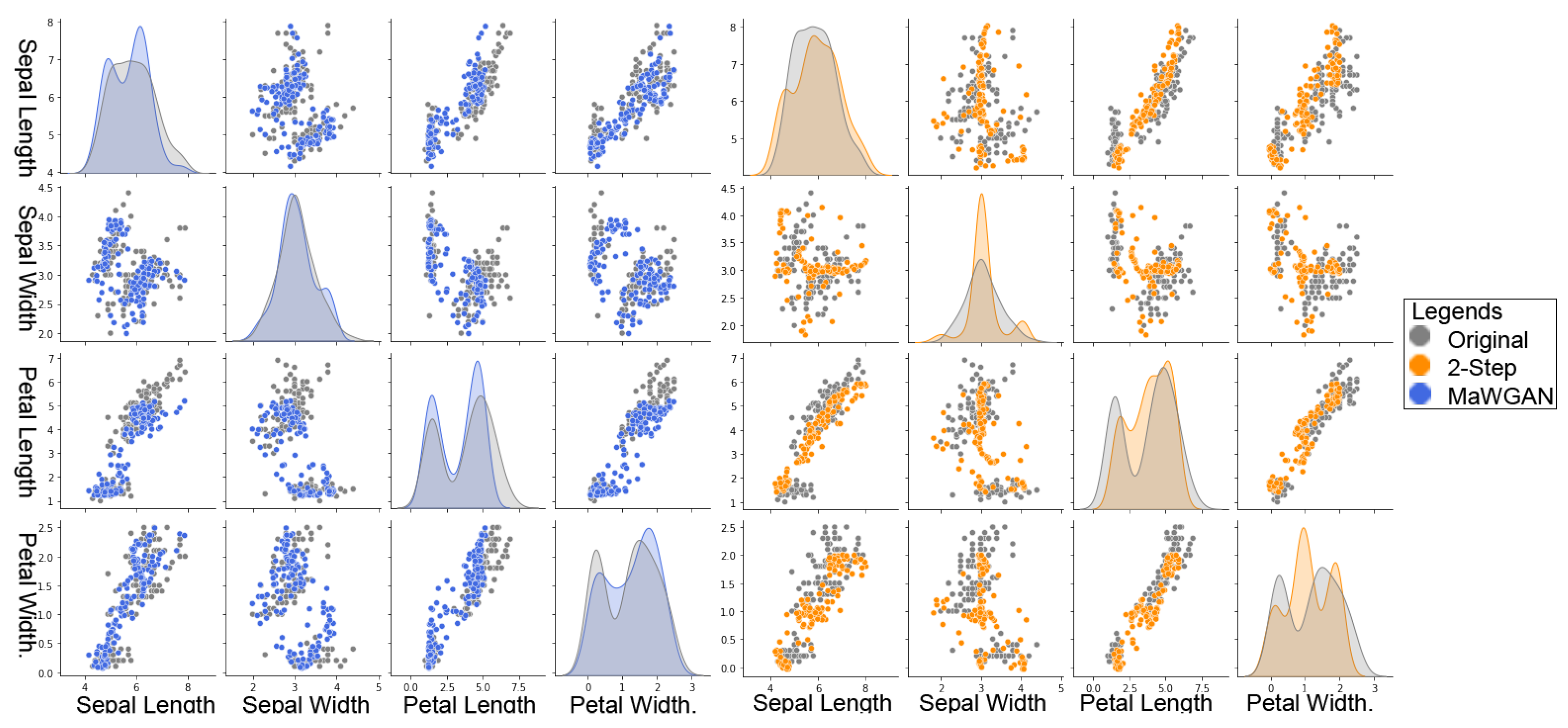
To get a better feel for the behaviour of each method, it is useful to directly compare the original data with a synthetic sample. In Figure 5, we feature the Iris dataset and use methods trained with 50% missing data. On the left, we have output from the MaWGAN, and on the right—from the two-step method. For each plot, we overlay the original data with a synthetic sample of the same size. We have four variables, and on the diagonal, we have for each a marginal density plot using a kernel smoother, and off the diagonal, we have pairs plots. Both methods have captured the location and scale of the data; however, the MaWGAN is noticeably better at picking up the bimodality.
5. Discussion
MaWGAN is a proper generalisation of WGAN-GP, since in the absence of missing data it is exactly a WGAN-GP, yet it requires no more parameter tuning than a WGAN-GP. Moreover the masking step that implements MaWGAN is simple to add to existing code, and has a marginal impact on the running time (calculating the weight-gradient for the generator and critic remains the most expensive steps). In particular, MaWGAN can use existing GPU-optimised code, such as the Torch library. We note that our theory and implementation apply equally well to the original WGAN formulation as the WGAN-GP approach, though we would always recommend the latter, as we have found its approach to training the critic much more stable.
Our experimental results indicate that compared to WGAN-GP, for dealing with data missing completely at random (MCAR), MaWGAN has a superior performance to the alternatives of separately imputing missing data or discarding incomplete observations, particularly with high levels of missing data. The two-step method of using GAIN to impute missing data, then WGAN-GP to synthesise data, performed essentially the same as MaWGAN with low levels of missing data. However the two-step method requires the fitting and tuning of two models, so it is slower, more prone to fitting error, and inherently more variable due to the additional variability introduced in the training of—and subsequent sampling from—the GAIN.
Clearly the performance of MaWGAN on data missing at random (MAR) is of interest and will require further testing.
Author Contributions
Methodology, T.P.-D. and O.D.J.; software, T.P.-D.; supervision, O.D.J. and Y.Q.; writing—original draft, T.P.-D.; writing—review and editing, O.D.J. and Y.Q. All authors have read and agreed to the published version of the manuscript.
Funding
This research was funded by a European Union KESS2 scholarship with support from Dŵr Cymru Welsh Water.
Informed Consent Statement
Not applicable.
Data Availability Statement
Iris dataset: https://archive.ics.uci.edu/ml/datasets/iris (accessed on 31 January 2022); WIMD dataset: https://gov.wales/welsh-index-multiple-deprivation-full-index-update-ranks-2019 (accessed on 31 January 2022); letter dataset: https://archive.ics.uci.edu/ml/datasets/letter+recognition (accessed on 31 January 2022).
Conflicts of Interest
The authors declare no conflict of interest.
References
- Rubin, D.B. Inference and missing data. Biometrika 1976, 63, 581–592. [Google Scholar] [CrossRef]
- Pigott, T.D. A review of methods for missing data. Educ. Res. Eval. 2001, 7, 353–383. [Google Scholar] [CrossRef] [Green Version]
- Troyanskaya, O.; Cantor, M.; Sherlock, G.; Brown, P.; Hastie, T.; Tibshirani, R.; Botstein, D.; Altman, R.B. Missing value estimation methods for DNA microarrays. Bioinformatics 2001, 17, 520–525. [Google Scholar] [CrossRef] [PubMed] [Green Version]
- Andridge, R.R.; Little, R.J.A. A review of hot deck imputation for survey non-response. Int. Stat. Rev. 2010, 78, 40–64. [Google Scholar] [CrossRef] [PubMed]
- Gold, M.S.; Bentler, P.M. Treatments of missing data: A Monte Carlo comparison of RBHDI, Iterative Stochastic Regression Imputation, and Expectation-Maximization. Struct. Equ. Model. 2000, 7, 319–355. [Google Scholar] [CrossRef]
- Yoon, J.; Jordon, J.; van der Schaar, M. GAIN: Missing data imputation using Generative Adversarial Nets. In Proceedings of the 35th International Conference on Machine Learning, Stockholm, Sweden, 10–15 July 2018; pp. 5689–5698. [Google Scholar]
- Azur, M.J.; Stuart, E.A.; Frangakis, C.; Leaf, P.J. Multiple imputation by chained equations: What is it and how does it work? Int. J. Methods Psychiatr. Res. 2011, 20, 40–49. [Google Scholar] [CrossRef] [PubMed]
- Campbell, M. Synthetic data: How AI is transitioning from data consumer to data producer… and why that’s important. Computer 2019, 52, 89–91. [Google Scholar] [CrossRef]
- Hitawala, S. Comparative Study on Generative Adversarial Networks. arXiv 2018, arXiv:1801.04271. [Google Scholar]
- Goodfellow, I.; Pouget-Abadie, J.; Mirza, M.; Xu, B.; Warde-Farley, D.; Ozair, S.; Courville, A.; Bengio, Y. Generative Adversarial Nets. In Proceedings of the Annual Conference on Neural Information Processing Systems, Montreal, ON, Canada, 8–13 December 2014; Ghahramani, Z., Welling, M., Cortes, C., Lawrence, N., Weinberger, K.Q., Eds.; Neural Information Processing Systems: La Jola, CA, USA, 2014; Volume 27 of Advances in Neural Information Processing Systems. [Google Scholar]
- Arjovsky, M.; Chintala, S.; Bottou, L. Wasserstein Generative Adversarial Networks. In Proceedings of the 34th International Conference on Machine Learning, Sydney, Australia, 6–11 August 2017; pp. 214–223. [Google Scholar]
- Gulrajani, I.; Ahmed, F.; Arjovsky, M.; Dumoulin, V.; Courville, A.C. Improved training of Wasserstein GANs. In Proceedings of the 31st International Conference on Neural Information Processing Systems, Long Beach, CA, USA, 4–9 December 2017; Guyon, I., Luxburg, U.V., Bengio, S., Wallach, H., Fergus, R., Vishwanathan, S., Garnett, R., Eds.; Neural Information Processing Systems: La Jola, CA, USA, 2017; Volume 30 of Advances in Neural Information Processing Systems. [Google Scholar]
- Dua, D.; Graff, C. UCI Machine Learning Repository; School of Information and Computer Science, University of California: Berkeley, CA, USA, 2022; Available online: http://archive.ics.uci.edu/ml (accessed on 31 January 2022).
- Anderson, E. The irises of the Gaspe Peninsula. Bull. Am. Iris Soc. 1935, 59, 2–5. [Google Scholar]
- Fisher, R.A. The use of multiple measurements in taxonomic problems. Ann. Eugen. 1936, 7, 179–188. [Google Scholar] [CrossRef]
- Welsh Government. Welsh Index of Multiple Deprivation (Full Index Update with Ranks). 2014. Available online: https://gov.wales/welsh-index-multiple-deprivation-full-index-update-ranks-2014 (accessed on 31 January 2022).
- Frey, P.W.; Slate, D.J. Letter recognition using Holland-style adaptive classifiers. Mach. Learn. 1991, 6, 161–182. [Google Scholar] [CrossRef] [Green Version]
- Guan, S.; Loew, M.H. Measures to evaluate Generative Adversarial Networks based on direct analysis of generated images. arXiv 2020, arXiv:2002.12345. [Google Scholar] [CrossRef]
- Borji, A. Pros and cons of GAN evaluation measures. Comput. Vis. Image Underst. 2019, 179, 41–65. [Google Scholar] [CrossRef] [Green Version]
- Borji, A. Pros and cons of GAN evaluation measures: New developments. Comput. Vis. Image Underst. 2022, 215, 103329. [Google Scholar] [CrossRef]
- Heusel, M.; Ramsauer, H.; Unterthiner, T.; Nessler, B.; Hochreiter, S. GANs trained by a two time-scale update rule converge to a local Nash equilibrium. Adv. Neural Inf. Process. Syst. 2017, 30, 6629–6640. [Google Scholar]
- Paszke, A.; Gross, S.; Chintala, S.; Chanan, G.; Yang, E.; DeVito, Z.; Lin, Z.; Desmaison, A.; Antiga, L.; Lerer, A. Automatic differentiation in PyTorch. In Proceedings of the 31st International Conference on Neural Information Processing Systems, Long Beach, CA, USA, 4–9 December 2017; Guyon, I., Luxburg, U.V., Bengio, S., Wallach, H., Fergus, R., Vishwanathan, S., Garnett, R., Eds.; Neural Information Processing Systems: La Jola, CA, USA, 2017; Volume 30 of Advances in Neural Information Processing Systems. [Google Scholar]
- Pytorch-Wgan. Available online: https://github.com/Zeleni9/pytorch-wgan (accessed on 31 January 2022).
Figure 1.
Flowchart for a single training step of the generator.

Figure 2.
Flowchart for a single training step of the critic.

Figure 3.
Likeness scores for each method on the three datasets with different levels of missingness (higher is better).
Figure 3.
Likeness scores for each method on the three datasets with different levels of missingness (higher is better).

Figure 4.
Fréchet distances for each method on the three datasets with different levels of missingness (lower is better).
Figure 4.
Fréchet distances for each method on the three datasets with different levels of missingness (lower is better).

Figure 5.
Original data compared with synthetic data from methods trained with 50% missing data: MaWGAN on the left and the two-step method on the right. In both cases, we overlay the original data with a synthetic sample of the same size. Marginal densities are given on the diagonals and pairs plots off the diagonal.


Table 1.
Overview of the advantages and disadvantages of some existing strategies for missing data imputation.
Table 1.
Overview of the advantages and disadvantages of some existing strategies for missing data imputation.
| Imputation Method | Accuracy | Computational Costs |
|---|---|---|
| Mean | Low | Low |
| KNN | Low | Med |
| Hot-Deck | Med | Med |
| Stochastic regression | Low-Med | Low |
| GAIN | High | High |
Table 2.
Number of complete observations remaining in each dataset after different proportions of data were removed at random.
Table 2.
Number of complete observations remaining in each dataset after different proportions of data were removed at random.
| Percentage Missing | Iris | Dataset WIMD | Letter |
|---|---|---|---|
| 0% | 150 | 1093 | 20,000 |
| 10% | 95 | 666 | 3723 |
| 20% | 57 | 218 | 564 |
| 30% | 35 | 59 | 67 |
| 40% | 16 | 11 | 5 |
| 50% | 5 | 2 | 0 |
| 60% | 1 | 0 | 0 |
| 70% | 0 | 0 | 0 |
| 80% | 0 | 0 | 0 |
| 90% | 0 | 0 | 0 |
Publisher’s Note: MDPI stays neutral with regard to jurisdictional claims in published maps and institutional affiliations. |
© 2022 by the authors. Licensee MDPI, Basel, Switzerland. This article is an open access article distributed under the terms and conditions of the Creative Commons Attribution (CC BY) license (https://creativecommons.org/licenses/by/4.0/).
Share and Cite
MDPI and ACS Style
Poudevigne-Durance, T.; Jones, O.D.; Qin, Y. MaWGAN: A Generative Adversarial Network to Create Synthetic Data from Datasets with Missing Data. Electronics 2022, 11, 837. https://0-doi-org.brum.beds.ac.uk/10.3390/electronics11060837
AMA Style
Poudevigne-Durance T, Jones OD, Qin Y. MaWGAN: A Generative Adversarial Network to Create Synthetic Data from Datasets with Missing Data. Electronics. 2022; 11(6):837. https://0-doi-org.brum.beds.ac.uk/10.3390/electronics11060837
Chicago/Turabian StylePoudevigne-Durance, Thomas, Owen Dafydd Jones, and Yipeng Qin. 2022. "MaWGAN: A Generative Adversarial Network to Create Synthetic Data from Datasets with Missing Data" Electronics 11, no. 6: 837. https://0-doi-org.brum.beds.ac.uk/10.3390/electronics11060837
Note that from the first issue of 2016, this journal uses article numbers instead of page numbers. See further details here.