Open-Source Software for Electromagnetic Scattering Simulation: The Case of Antenna Design


1
Department of Electrical, Electronic, Telecommunications Engineering, and Naval Architecture, University of Genoa, Via all’Opera Pia 11A, 16145 Genoa, Italy
2
Atel Antennas S.r.l., Viale Caduti sul Lavoro 35, 15061 Arquata Scrivia, Italy
*
Author to whom correspondence should be addressed.
Electronics 2019, 8(12), 1506; https://0-doi-org.brum.beds.ac.uk/10.3390/electronics8121506
Submission received: 30 October 2019
/
Revised: 4 December 2019
/
Accepted: 5 December 2019
/
Published: 9 December 2019
(This article belongs to the Special Issue Computational Electromagnetics and Its Applications)
Abstract
:Electromagnetic scattering simulation is an extremely wide and interesting field, and its continuous evolution is associated with the development of computing resources. Undeniably, antenna design at all levels strongly relies on electromagnetic simulation software. However, despite the large number and the high quality of the available open-source simulation packages, most companies have no doubts about the choice of commercial program suites. At the same time, in the academic world, it is frequent to develop in-house simulation software, even from scratch and without proper knowledge of the existing possibilities. The rationale of the present paper is to review, from a practical viewpoint, the open-source software that can be useful in the antenna design process. To this end, an introductory overview of the usual design workflow is firstly presented. Subsequently, the strengths and weaknesses of open-source software compared to its commercial counterpart are analyzed. After that, the main open-source packages that are currently available online are briefly described. The last part of this paper is devoted to a preliminary numerical benchmark for the assessment of the capabilities and limitations of a subset of the presented open-source programs. The benchmark includes the calculation of some fundamental antenna parameters for four different typologies of radiating elements.
1. Introduction
Numerical simulation applied to electromagnetic scattering problems represents a very broad and multifaceted field. Historically, its bases derive from the initial attempts to find numerical solutions for describing electromagnetic propagation phenomena in complex and realistic scenarios, where analytical calculations were inapplicable. Throughout the years, the enormous increase in the available computer power, as well as the benefits of hardware task parallelization, have brought the electromagnetic simulation to a new era. Simultaneously, the worldwide availability of Internet connections, as well as the widespread diffusion of information and communication technologies, have removed all the barriers in opening science [1].
In this fast-growing background, the use and the development of numerical software for electromagnetic simulation follow two main directions.
- In the industrial world, the standard approach is to employ commercial software suites, because of their easy integration in the design workflow, as well as their extended support and documentation.
- In the academic world, it is very frequent to develop in-house simulation software from scratch, or alternatively to modify existing software packages in order to experiment new models and algorithms. In other words, the development of electromagnetic simulation software is still a wide research field itself, as witnessed by many recent papers on this topic (e.g., [2,3,4,5,6,7,8,9,10,11,12]). Of course, for advanced and high-level simulations, the use of commercial programs (sometimes combined with academic/research licenses) is customary.
However, in both situations, the knowledge of the existing open-source possibilities is often scarce. In both academic and industrial frameworks, especially when the available budget is rather low, it is more common to find illegal versions of commercial software suites rather than move to their open-source counterparts. Of course, this creates an important ethic problem, which is also accompanied by a series of potential security concerns.
Moreover, it is very rare that more than one academic institution work together for the practical development of open-source simulation packages, and it is more than rare that both universities and companies work together on that. The only exception is represented by several public-funding research projects at national or international levels. However, when such projects come to an end, these joint efforts encounter significant difficulties.
We are not here to prove the superiority of open-source software with respect to commercial products. Clearly, the better usability, reliability, and computational efficiency of commercial software packages are so far undeniable, and, therefore, will not be discussed in these pages.
We only believe that a proper knowledge of the existing open-source alternatives can be very useful for researchers working in this field. From the point of view of graduate and undergraduate students and their teachers, open-source software can assume an important role in their educational path. Furthermore, it should be stressed that an up-to-date view of the available open-source packages can be beneficial even for the developers of commercial electromagnetic software houses. Cultural motivations also exist: in the research and scientific community there is nowadays an increasing demand of open data, results, algorithms, and codes [13].
It is easy to understand that a comprehensive review of open-source packages is a huge work, and cannot be resolved from a unique perspective. The goal of the present paper is to review open-source software in electromagnetic scattering simulation, and in particular to identify possible open-source programs that can be fruitfully used in the design of antennas and its workflow. Another aim of this research is to evaluate the pre- and post-processing capabilities of the open-source packages. It should be clear that this work is not intended as a compared validation of various software implementations, and the main target of this review is not to select a problem formulation, a simulation method, or a software package with respect to others. On the one hand, computational electromagnetics (CEM) software should be primarily compared based on computational or result quality merits, and in this field, the potentialities of the different packages are often problem-dependent. On the other hand, the form of ownership and user experience are not scientific criteria in a strict sense, but these factors influence software diffusion and should not be neglected: open-source packages achieve a widespread distribution where usability is taken into account.
As a result, this review is organized as follows. A first distinction between open-source and free software is given in Section 2, for the readers that are unfamiliar with the subject. In the subsequent Section 3, some basics for a general understanding of the antenna design workflow are provided. After that, an overview of the different calculation methods, along with some strengths and weaknesses of open-source and commercial software packages, are presented in Section 4. The subsequent Section 5, Section 6 and Section 7 are devoted to a first description of the main open-source programs that are currently available. A preliminary numerical assessment, in which a subset of the presented packages has been evaluated, is reported in Section 8. In particular, an initial benchmark composed of four different kinds of antenna structures is taken into account. Results are discussed and compared in Section 9. Finally, Section 10 draws some concluding remarks.
2. Open-Source Programs and Free Software
To start with, a first distinction should be made between open-source codes (and free, according to the definition given by the GNU project [14]) and software whose access is free of charge, but still remains proprietary.
The programs belonging to the first family are also released with their source code, which can be freely studied, modified, and customized to the user’s needs. However, it is worth noticing that some restrictions can apply to the redistribution of modified versions of the software.
The second family of software is characterized by only a binary distribution of the packages, and therefore no changes by the user (e.g., integration, porting, modification, etc.), as well as no access to their sources, are allowed.
This paper is focused on open-source software. Hence, other programs, which can be found on the Internet for free but are available only in binary closed-source form, are not discussed here.
3. Design Workflow
In general, the workflow of any device is a complex process, made of many different phases, that could be reiterated until a satisfactory result is obtained. A simplified sketch of the antenna design workflow, in which hardware prototyping and the subsequent steps are not included, is reported in Figure 1.
Without entering in all the details, from the point of view of the electromagnetic simulation, three subsequent phases in the design process of antennas and electromagnetic devices can always be identified. According to the common terminology, we have:
- Pre-processing;
- Solution of the electromagnetic problem, by means of a proper numerical “engine;”
- Post-processing.
3.1. Pre-Processing Phase
The goal of the pre-processing phase is to translate the initial idea of the actual object into an approximate computer model, compatible with the numerical solver. This phase can be in turn decomposed in various steps. The most significant are:
- Description of the geometric parameters of the design;
- Approximation of the geometry by means of a proper modeling tool, through the generation of a (structured or unstructured) mesh. In this way, the device is decomposed into elementary building blocks;
- Description of the physical parameters; definition of the sources and choice of the correct model;
- Final definition of the simulation model;
- Generation of the input data for the solver engine.
To carry out these steps, the user can interact with the software either with a graphical user interface (GUI) or by writing a text file in a specific scripting language. A mix of these two approaches is also possible. Furthermore, during this pre-processing phase, the documentation useful for the production of the device may be generated (e.g., drawings, layouts, part list, etc.).
3.2. Solution Phase
In this phase, the data generated during the pre-processing step are supplied to a solver engine, in order to obtain the numerical solution of the electromagnetic problem. The solver will generate one or more output files containing the results, to be used in the post-processing phase.
3.3. Post-Processing Phase
In the post-processing phase, the requested data are extracted from the output files provided by the numerical solver. In this case, too, the operations can be defined with a graphical interface, or by using a command script.
The collected data may be organized in files, tables, or graphs, and will be used for different purposes. Of course, the first purpose is the verification of the result. However, the output data may be also used to complete the documentation (both internal and public), to perform comparisons with other simulations and/or similar devices, or even to generate input data for other simulations.
An additional objective of the post-processing may be to generate the documentation needed for the production of the device, if not yet created during the pre-processing phase.
4. Calculation Methods
The most common calculation methods adopted for the electromagnetic simulation can be subdivided into several classes, based on the kind of numerical approximation of Maxwell’s equations. Moreover, both methods operating directly in time domain and single-frequency approaches exist.
Not all the possible numerical methods are implemented in an open-source version. As regards antenna design, the choice is essentially limited to two methods: the Finite Difference Time Domain method (FDTD) and the Method of Moments (MoM, implemented in the frequency domain). A third approach, which is widespread in the open-source community for the solution of complex equations, i.e., the Finite Elements Method (FEM), is usually implemented in multi-physics packages not necessarily focused on electromagnetic applications, and at the present time, it does not appear sufficiently mature for an open application in electromagnetics. However, some promising FEM codes are briefly discussed in Section 7. A more deep discussion about the cited methods, as well as their open-source implementations, will be presented in the following sections.
It should be noted that it is quite difficult to describe methods’ formulations with a correct level of detail in the framework of this review, especially for the most advanced techniques. In addition, there would be a risk of repetitions with respect to the existing scientific literature. For these reasons, we decided to provide some key references to theoretical works on modeling formulations instead of replicating part of their content and equations. For readers interested in the mathematical bases of the presented methods, several very good books exist where the most common formulations are presented, discussed and compared [15,16,17,18]. These books may be very useful for educational purposes, too.
Advantages and Disadvantages of Commercial and Open-Source Products
It is to dispel the common opinion that open-source packages are in all cases worse than their commercial counterparts. In particular, when electromagnetic simulation is concerned, open-source software is usually very rigorous and formally correct from both the mathematical and the numerical points of view. Nevertheless, it is true that open-source packages for electromagnetics are less versatile and they lack most of the ancillary tools typical of commercial products. This is mainly due to the relatively young and niche field, even for the open-source community: the result is a slow development of complete packages for electromagnetic calculations. Despite these facts, several packages that can be fruitfully used—and in constant development—exist.
In general, high-level commercial products contain all the tools required for the whole design workflow. Conversely, they are characterized by high costs for buying and maintaining the license. It is worth noting that student versions of commercial simulators are often available, but they are significantly limited (with few exceptions) and do not allow professional usage. Academic versions may be also available (free of charge, in few cases, or with noticeable discounts) but their license is quite restrictive and their use outside non-commercial research purposes is prohibited. A rough and not-exhaustive list of pros and cons related to commercial packages is reported in Figure 2.
At present, the use of open-source software for electromagnetic simulation requires the integration of inhomogeneous products, which seldom offer the same level of functionality. If a complete system is needed (i.e., including pre-processing, solver engine, and post-processing) it is sure that several open-source packages should be integrated together with other “homemade” modules. However, the possibility of accessing source codes and the existence of good developers communities sometimes allow the user to solve problems quicker than with commercial products. A concise list of key points about open-source software in electromagnetics, describing some pros and cons, is reported in Figure 3.
5. Method of Moments
Historically, Method of Moments [19,20] is the first kind of solvers for which the initial open-source applications were developed. The most famous code that implements the MoM is the NEC-2 [21]. Most of the MoM applications are developed in the frequency domain, and the open-source world is not an exception. In fact, all the programs described in the following sections have been elaborated starting from Maxwell’s equations in the frequency domain.
5.1. NEC-2 and Derived Programs
The reference program for many open-source applications of the MoM is NEC-2 [21,22]. The NEC-2 code is based on the so-called thin-wire kernel [23], where only axial currents are considered and modeled according to a three-term expansion that was proposed by Yeh and Mei [24]. This approach implies that NEC-2 is limited to the modeling of structures composed of metallic wires or tubes. Furthermore, although wires could be also connected by means of lumped elements networks or transmission lines, the surrounding environment should be vacuum (free space) or, at most, a half-space. Therefore, antennas and devices containing dielectric parts cannot be simulated, even though in the past the code was employed for simulating the emissions radiated by printed circuit board tracks [25]. When metallic plates have to be modeled, they are approximated with a grid of wires [26,27,28]. There are also some limitations about the positioning of intersections and reciprocal positions of wires, that have been highlighted through the years.
Despite these limitations, this software program is successfully adopted for the analysis, the design, and the validation of various kinds of antennas. To cite some examples, Olver and Sterr used NEC-2 for validating the project of a corner reflector antenna developed with the FDTD method [29]. NEC-2 has also been used for the calibration of antennas for electromagnetic compatibility [30,31], as well as for the modeling of lightning [32] and transient over-voltages [33]. NEC-2 code has also found interesting applications in radio astronomy, in particular for projects related to low-frequency radio-telescopy [34,35]. The use of NEC-2 as a simulation engine in optimization processes has been proposed for the project of generic wire antennas [36], as well as for the optimization of the parameters of dipole arrays [37] and the design of logarithmic-periodic antennas [38]. In the field of arrays, around the NEC-2 program algorithms for the estimation of the direction of arrival (DOA) have been also developed [39].
The original NEC-2 source code, developed in Fortran, is currently available, as well as are the C and C++ porting of the code.
Presently, no modeling software or other programs for the generation of input data are available. In addition, there is a limited possibility of post-processing the output data by using open-source packages. On the other hand, a huge variety of ready-made antenna models can be found over the Internet. These models are useful as the starting point for antenna design.
Among the most interesting software packages that exploit the NEC-2 engine, we highlight:
- nec2c [40]
- It is a C porting of the original source code; it has been widely tested and can replace the original code without problems. Differently from the original Fortran code, it allows command line input/output and dynamically allocates the resources (there is no need to recompile the application if the predefined memory is not sufficient).
- necpp [41]
- It is also known as nec2++, it is the C++ porting of the original source code; it may be interesting since the program has been restored and it is organized around a library that can be called from C, C++, Python and Ruby codes.
- xnecview [42]
- It is a program for visualizing input and output data. Regarding input data, it allows the user to visualize the analyzed structure; at the output, it provides the radiation pattern in two and three dimensions, the input impedance, the voltage standing wave ratio (VSWR) and the maximum gain with respect to frequency. This program can export graphs as image files, but it cannot create files and tables containing numerical values. The program code is rather difficult to understand.
- xnec2c [43]
- By partially using the xnecview code, the nec2c developer realized an application for visualizing and modifying the project in an interactive way. Unfortunately, the program has no textual output in the numerical format, but only a visual one. However, in the latest versions, it is possible to export some data not only as images but also as a file to be handled with the well known graphing utility gnuplot [44].
The NEC-2 has evolved in versions 3 and 4. These codes have been classified for a long time and presently are not available free of charge. Nevertheless, it seems that the classifications constraints have been removed almost completely and that now the NEC-4.2 source code can be obtained for a fee [45].
5.2. MiniNEC3
Despite the very similar name, the MiniNEC software package is structurally different from NEC-2 [46] as regards the numerical model, the implemented code, and the input/output. The original code, written in an old version of the BASIC programming language, is still available nowadays [47]. According to some users, the behavior of MiniNEC is better than NEC-2 for handling wires very close together and junctions between wires with different diameters.
5.3. Puma-EM
Puma-EM [48] is a software package developed in order to study the Radar Cross Section (RCS) of perfectly conducting structures. It is based on the Boundary Element Method (BEM) [49,50] together with a Multilevel Fast Multipole Method [51]. It is capable of computing the monostatic and bistatic RCS and to perform Synthetic Aperture Radar (SAR) calculations in the presence of perfectly electric conducting (PEC) targets. These targets can include junctions (e.g., plates intersected with volumes) and therefore the code can be applied to complicated geometries. Puma-EM does not have the necessary characteristics to model transmitting antennas and for retrieving their input parameters but is able to evaluate their radiation pattern. The software package has the attracting feature of accepting, as geometric input models, files generated by Gmsh [52], a mesh-generator program well known in the open-source world.
5.4. SCUFF-EM
SCUFF-EM [53,54] (or scuff-em) is a software suite based on the BEM [49,50]. The acronym stands for Surface-CUrrent-Field Formulation of ElectroMagnetism. The implementation is very accurate: in particular, the author and his collaborators paid attention to the development of an efficient method for calculating the integrals involved in the BEM formulation [55]. The program is well documented, although some parts of the documentation are incomplete.
SCUFF-EM was born with the original intention of studying highly specialized phenomena in photonics, such as the Casimir forces or the radiative transfer [56,57,58,59]. However, it evolved in a complete suite for the BEM analysis of electromagnetic scattering for nanophotonics, RF/microwave engineering, electrostatics, and so on [58]. It includes a main library with a low-level C++ application program interface (API) and many command-line applications, each one developed for dealing with particular electromagnetic problems.
The most interesting ones, as far as RF design is concerned, are scuff-scatter, a generic application for the study of electromagnetic scattering, scuff-static, specialized for electrostatics, and mostly important scuff-rf.
The open-source package SCUFF-EM also includes a general high-level application (scuff-solver) that exposes the functionalities developed in the single modules, with an interface that can be called from C++, Python, and MATLAB applications.
For the definition of geometric entities and the corresponding meshing operations, SCUFF-EM uses the Gmsh software [52]. Moreover, it can also perform complex operations on the generated meshes, such as translations, rotations, duplications, etc.
5.5. Buff-em
Buff-em is complementary to the SCUFF-EM software since it implements some cases that are not included in SCUFF-EM. In particular, these cases are characterized by the presence of inhomogeneous dielectric materials (SCUFF-EM can deal with piecewise homogeneous materials only) and anisotropic materials. Buff-em implements the solution of Maxwell’s equations based on volumetric currents using SWG basis functions [60]. The implementation of Buff-em is also very accurate [61]. However, at present, Buff-em is not as rich of capabilities as SCUFF-EM. Although the Buff-em library offers analogous functionalities as SCUFF-EM, so far only the scattering module and a program for Casimir forces and radiative heat transfer [62] are already implemented as independent command line tools. Moreover, as the software author says, Buff-em is significantly slower than SCUFF-EM when both software packages can be used for the solution of the same problem. We also notice that, due to the adopted implementation choices, Buff-em cannot deal with surface currents, and therefore it cannot model PEC objects.
6. Finite Difference Time Domain Method
Most open-source software of recent development is based on the FDTD method. There are some variants of the method, but all the current implementations are based on the so-called “leap-frog” scheme proposed by Yee in 1966 [63,64]. FDTD has since become very popular and many high-level textbooks can be found about the method (see for example [17,65]). In addition, a comprehensive, high-quality book available in open source can be found [18]. The FDTD method seems to offer at least two great advantages compared to the MoM: it does not require the inversion of large data matrices (therefore, it is quite limited in memory requirements) and it is able to evaluate antennas in a wide frequency band with a single simulation in the time domain. Obviously, the method has also some disadvantages, such as the need of approximating the model geometry on regular grids. Despite this one and other well-known limitations [17], FDTD is widely used even in commercial products.
Among the most interesting open-source implementations we find OpenEMS [66], GprMax [67], and Meep [68]. However, it is worth to analyze also other packages like Vulture [69], Angora [70], and GS-Vit [71].
6.1. OpenEMS
Actually, the openEMS program [66] is the solver of a suite of well-integrated applications [72] for the geometric modeling, the solution, the generation of output data in different formats, and the integration of the circuit simulation of electromagnetic systems and apparatuses. Basically, the suite is composed of four tools, integrated with each other.
CSXCAD is a library which allows the user to define various elementary geometric entities, and operate with them by means of the typical operations that can be found in computer graphics applications (rotations, translations, duplications, extrusions, masks, etc.). Both graphical and physical properties (e.g., dielectric permittivity) can be added to each object. Differently from other modeling tools, the CSXCAD library has been probably conceived from the beginning for the use with electromagnetic simulation. Therefore, it is possible to define particular properties inside the model, e.g., Drude, Debye, or Lorentz behaviors, as well as to insert lumped elements and test points. The CSXCAD library takes care of the mesh generation and the problem discretization. In this respect, it is worth noticing that the openEMS suite can handle non-uniform meshes, and CSXCAD includes some routines for the semi-automatic generation of meshes with non-uniform spacing and accurate smoothing. Furthermore, CSXCAD contains an interface package to be used with Octave/Matlab.
QCSXCAD extends CSXCAD with a section devoted to the generation of GUIs, and AppCSXCAD is a graphical tool using the QCSXCAD library. Although AppCSXCAD should theoretically allow the complete graphical handling of the definition and generation of the simulation space, presently the interface is relatively poor and not very comfortable for the user. However, this interface turns out to be particularly interesting for the visualization of geometries (including feed ports, probes, and lumped elements) and for exporting the model in other graphical formats for the visualization with external software (e.g., Paraview [73] or Povray [74]).
The core program of the suite, openEMS, is based on the EC-FDTD method [75,76]. The method has been originally developed in the field of MRI (Magnetic Resonance Imaging) [77,78], but it is completely general. Examples of the use of the package in the field of antennas and arrays can be found in [79,80,81]. It is worth noting that openEMS has been also successfully employed in advanced biophysical research [82].
6.2. GprMax
The gprMax software [67], as the name suggests, was born for the electromagnetic simulation in the frame of ground penetrating radar (GPR) applications. However, nowadays it can be properly considered as a general-purpose simulator.
The last version of gprMax is written in Python language (version 3) and the most critical sections for the computing performance are implemented in Cython [83]. The program not only includes a parallel solver based on the OpenMP libraries, but it is also one of the few packages (among the ones discussed in this document) that can actually exploit the computing power of an Nvidia GPUs [84].
The development of gprMax is very accurate, and great attention is paid to the theoretical correctness of the employed algorithms. Among the possible feed ports, gprMax also includes a “virtual” transmission line [85] which, as the developers say, should avoid most of the perturbations introduced in simulation models by other kinds of ports (e.g., lumped element ports).
The history of the development of this software package can be summarized through some papers by the developers [86,87,88]. More references can be found on the gprMax website [83]. On the same site, there is also a summary of the many research papers whose development was based on gprMax. According to this list, gprMax is cited by more than 500 scientific papers.
Being written in Python, gprMax is intrinsically capable of interfacing with all the Python world, and itself is also written as a Python package. As regards the post-processing phase and visualization of results, some examples of using the open-source graphing package matplotlib [89] are included in the source code. Moreover, the output files (both geometries and results) can be easily read with Paraview [73], by using a macro that can be found on the gprMax website.
6.3. Meep
Meep [68] is a program that was born in the framework of advanced optics and is likely to be the most advanced among open-source FDTD programs. It is fully scriptable by using the Scheme language, in C++ and Python. The package contains advanced tools for both simulation and post-processing and has been used in photonics [90,91] but also for the optimization of patch antennas [92].
Nevertheless, due to the functional complexity, the learning curve of the Meep simulator is rather steep, especially when the user wants to move outside the photonic applications (for which several examples exist) to simulate antennas and other conventional devices at radio ad microwave frequencies.
6.4. Vulture
6.5. Angora
6.6. GS-Vit
GSvit [71] includes a set of numerical tools for the FDTD simulation, with the additional support for graphics cards compatible with the Nvidia CUDA (Compute Unified Device Architecture) environment [97,98]. The main scientific purposes include research in the field of nanotechnology and nanoscale optics, as well as near-field scanning microscopy, Raman scattering, scattering from rough surfaces, etc. However, as the FDTD method is universal, it can be used in principle for any other scope.
7. Finite Element Method
FEM codes and libraries are largely represented in the open-source world [99] and are of common use in many fields of engineering, especially in structural analysis, fluid dynamics, and heat transfer problems, but also in CEM. Moreover, FEM is the preferred kind of mathematical discretization in multi-physic problems. Nevertheless, finite element methods are, on the contrary, not so common in antenna design. One of the main reasons limiting the use of open source FEM packages is that most of these packages offer general-purpose solvers, requiring a further time-consuming and specialist programming, to implement the solution model. In general, the approach is slightly easier for the closed domain where PML or similar open-boundary conditions are not needed (for example for Surface Impedance Boundary Conditions [100,101]). Furthermore, using localized sources (ports) is another crucial point, because, in general, they are not available (except very simple cases, like elementary dipoles) in the codes and must be designed together with the model. However, there are some projects that deserve attention. We mention, in particular:
- deall.ll [102]
- It is a C++ library to construct Finite Element models. In its web site, there are some examples of electromagnetic problems.
- FEniCS [103]
- The FEniCS Project aims at creating mathematical methods and software for automated computational mathematical modeling by using finite element methods. The use of FeniCS in electromagnetic applications is discussed in [104].
- BEM++ [105]
- It is not a FEM library. It is instead a Boundary Element library, which has been used to face problems modeled with Maxwell and/or Helmholtz equations. It is cited in this section, as it can be interfaced with FEniCS, to describe coupled FEM-BEM problems.
- Elmer [106]
- Elmer is a multi-physical simulation software that was made open-source in 2005. Among the many modules available, it contains a solver for the time-domain wave equation and a solver for the vector Helmholtz equation. Unfortunately, there is no literature (to the authors’ knowledge) about such modules and also the internal documentation is very limited.
- ONELAB [107]
- ONELAB (Open Numerical Engineering LABoratory) is a complete environment for pre-processing, solving and post-processing, based on the mesh generator and post-processor Gmsh [52] and on the solver GetDP [108,109]. On the website of ONELAB [110] some references to simple examples of antenna models can be found.
- XLiFE++ [111]
- XLiFE++ (eXtended Library of Finite Elements in C++) contains solvers for Helmholtz and Maxwell equations.
- FreeFEM [112]
It should be stressed again that none of the previous packages provide a “ready-to-use” user program, but a notable programming effort is still needed to define the problem and model of the solution.
8. Numerical Assessment
A fair comparison of the existing open-source electromagnetic simulation software that can be used for antenna design is quite difficult for three main reasons. First, suitable testing benchmarks should be defined. Second, the post-processing phase of open-source software is often non-homogeneous, and therefore not all the relevant parameters may be directly provided in output by all packages. Third, because of the free nature of open-source programs, all-inclusive and cross-platform installation utilities are almost never provided. As a result, installation and compatibility issues frequently arise, and it is sometimes difficult to run programs that—in principle—are very powerful.
As a preliminary assessment, we chose to present the results obtained by three open-source packages: nec2c, gprMax, and openEMS versus some commercial and academic software alternatives based on MoM formulations. An extended comparison including the other presented open-source programs is under development.
To start with, simple canonical structures are considered. Four different antennas have been simulated here: a standard half-wavelength dipole, a circular loop antenna, a radiator composed by a metallic box and a plate, and finally a patch element on a dielectric substrate. The first examples have been inspired by a set of numerical benchmarks proposed in the IEEE recommended practice for the validation of CEM computer modeling and simulations [115] and in [116]. All the antenna geometries have been visualized here by processing with Paraview 5.6.0 [73] the meshes obtained with gprMax, but analogous results may be achieved by using other packages. Results in the frequency domain are retrieved from the time-domain simulators (gprMax and openEMS) by performing a Fast-Fourier Transform (FFT) on the simulated data.
8.1. Half-Wavelength Dipole
A simple half-wavelength dipole made to resonate around 500 MHz has been considered first. Its geometry, shown in Figure 4, is composed of a z-directed thin cylindrical shape with an overall length mm, subdivided into two arms by a gap of mm width. The antenna material is assumed as PEC.
It is worth noting that the nec2c code, which is based on an MoM formulation, does not require the discretization of the surrounding space, but only of the antenna element. Conversely, the two FDTD codes gprMax and openEMS need to build a simulation region around the antenna in which even the free space is discretized, and surrounded by proper absorbing boundary conditions.
The gprMax simulation involved a region of space of dimension m, discretized with 2 mm voxel size ( cells). The antenna is located at the center of this region, and it is fed by a 50 z-directed transmission line port excited with a Gaussian waveform with the central frequency equal to 1 GHz. A perfectly matched layer (PML) of 10-cells width encloses the simulation domain. The simulated time window has a width of ns, with a time step equal to ps (25,964 iterations).
In the openEMS simulation, a domain of the same size as in the gprMax simulation has been considered, with also the same depth of the PML layer. Using the capability of openEMS to deal with non-uniform meshes, the domain was discretized into FDTD cells, and the simulation resulted in a time step of ps. The simulated time window has a width of ns (26,000 iterations).
The considered antenna structure can be simulated by employing different kinds of numerical models. For instance, thin wire or cylindrical models can be adopted. The wire model is the simplest one and represents the antenna as a wire (or an edge) in the simulation mesh. As previously mentioned, the open-source nec2c software can only deal with wire models. With nec2c, the simulation was carried out by considering a wire of radius mm, divided into 151 uniform segments. This is about the same wire model used in the original benchmark [116], where the segments are 150 and a small gap is left for feeding the structure. The magnitude of the reflection coefficient measured at the antenna port has been reported in Figure 5a, where the open-source software is compared with a wire-model simulation obtained by two commercial software packages. Moreover, the analytic solution in the case of a sinusoidal current distribution has been reported in this graph [117].
A good agreement is observed between the computed reflection coefficients. The real and imaginary parts of the complex impedance measured at the antenna port versus frequency are also shown in Figure 5c,e, respectively, where the same comments as before still hold. In all cases, there are relevant differences between the analytic solution and the numerical ones around 1 GHz and 2 GHz, where the theoretical impedance computed with the sinusoidal current approximation tends to infinity [117] since the length of the dipole l is a multiple of the wavelength in free space.
The compared simulation results achieved with a cylindrical model of the same dipole, where the arms are represented with a cylinder of diameter mm, can be found in the same figure. In particular, Figure 5b reports the reflection coefficient magnitude, whereas the complex impedance is shown in Figure 5d,f.
In general, results are quite similar; the only significant differences are noticed for the impedance calculation by means of the second commercial code. A small underestimation of the impedance values is also observed in the gprMax simulation. These differences in results may be ascribed to the different modelling capabilities of the adopted simulators, and in particular to the staircase effect in the uniform FDTD mesh.
Moreover, the gain of the antenna obtained with nec2c compared with a commercial program and the analytic solution [117] is reported in Figure 6, in case of a thin wire dipole. It is evident that these results match exactly. Unfortunately, not all the software packages implement near-field to far-field (NFFF) transformations (e.g., gprMax) and therefore the radiation pattern is not always available. This may be a limitation of some open-source programs for the design and characterization of antennas in far-field conditions.
8.2. Loop Antenna
As a second example, a circular loop antenna has been considered, which is represented in Figure 7a. The loop has a diameter mm and the cylindrical PEC wire has a thickness mm. The radiating structure is fed through a gap of width mm.
The nec2c simulation of the loop antenna was based on the discretized wire loop provided with the results of [116]. Once again the wire was divided into three segments to position the feeding port. The gprMax software has been run with a domain of side lengths m, enclosed by a 10-cells PML boundary. A uniform mesh with 2 mm voxel size has been chosen, with a resulting total number of cells equal to . Like in the previous case, the antenna is centered within the simulation domain, and it is fed by a 50 z-directed transmission line port. The structure is excited with a Gaussian waveform characterized by a central frequency of 300 MHz. A time window of width ns has been considered, with a time step equal to ps (25,964 iterations).
The magnitude of the reflection coefficient at the port of this antenna versus frequency can be seen in Figure 7b. In can be seen that the superposition of the three results is almost perfect. The corresponding real and imaginary parts of the complex input impedance are reported in Figure 7c,d. In these graphs, some differences can be appreciated among the results. There could be many possible causes for these behaviors, but the more obvious and probable is that the initial dissimilarities in the geometrical and electromagnetic models can give rise to these small differences in the results.
Figure 8 shows an -plane cut of the antenna gain, where the nec2c simulation is compared with a commercial package. The trend is similar, but a maximum difference of 1 dB is evident in the left lobe of the pattern, which corresponds to the location of the feed point. This must be investigated; however, it can be guessed that the different model of the feeding port could be the reason for this difference. The problem of accurately modeling the ports is still a challenging task for any simulator, both open-source and commercial.
8.3. Box-Plate Antenna
A more complex antenna configuration has been taken into account, as shown in Figure 9. In particular, the structure is composed of a square PEC plate at the bottom (whose side length is mm) and a metallic box on the top (again, for more details, the reader is referred to [116]). The box has dimensions mm, mm, mm, and it is separated from the bottom plate by a distance mm. Particular attention should be paid in this case to the feed point, whose details are visible in Figure 9b. A small metallic box is attached to the upper part of the antenna, in the central position, and its dimensions are mm, mm, mm. The resulting gap between the box and the PEC plate is mm.
In the gprMax simulation, the simulation domain and the time window have the same size as in Section 8.2. However, due to the increased complexity of the structure, a spatial discretization with 1 mm voxel size has been adopted. As a result, the simulation domain contains cells, and the time step is reduced to ps (51,927 iterations). As shown in Figure 9b, since the spatial discretization is smaller than the gap between the plate and the box, a PEC edge has been placed to fill the space between the gprMax transmission line (which is in contact with the bottom plate) and the box.
The openEMS simulation has been carried out by using the same domain size as in gprMax simulation, the same depth of PML and fixing the minimum acceptable resolution to at 6 GHz. This resulted in a domain discretized into FDTD cells, with a time-step ps and a total excitation length of , corresponding to a Gaussian modulated pulse with a dB band GHz.
A comparison between the simulated magnitude of the reflection coefficient versus frequency is presented in Figure 10. A very good agreement between the various electromagnetic solvers is observed, despite the complexity of the structure. Moreover, these results match very well with the experimental measurements reported in [116].
8.4. Patch Antenna
At the end of this preliminary assessment, a rectangular patch antenna has been simulated. The structure, presented in Figure 11, is supported by a dielectric substrate Rogers RT/Duroid 5880 (characterized by a relative dielectric permittivity ) with length mm, width mm and thickness mm. A PEC plate, with the same length and width of the substrate, is assumed at the bottom. The patch element has a rectangular shape of length mm and width mm. The antenna is fed by a vertical edge placed inside the substrate between the bottom conducting plane and the upper patch. The feed point is centered on the y-axis, whereas on the x-axis is off-centered by an offset mm.
The gprMax simulation of this antenna has been made by considering a box of size mm. A PML absorbing layer is placed on the external boundary of the simulation domain, as usual. A Gaussian pulse whose spectrum is centered at 10 GHz has been used as the excitation waveform, and the simulated time window is ns wide. A transmission line is placed inside the substrate dielectric material.
In this case, a comparison has been done between gprMax and openEMS results obtained with two different spatial discretizations. In the first simulations, a coarse spatial discretization with 1 mm voxel size has been employed ( cells) with a time step ps (51,927 iterations). In the second case, a finer spatial discretization of 0.5 mm ( cells) has been used, adopting a time step equal to ps (103,853 iterations). Like in Section 8.3, in this case, the transmission line is in contact with the bottom plate, and a vertical conducting edge lies between the transmission line and the upper patch element.
As for openEMS, again the capability of using non-uniform meshes has been used to refine some details of the simulation, however, in order to compare results, the simulation domain was taken as much as possible similar to the one used for gprMax. In particular, the dimensions of the simulation volume and the number of PML layers were exactly the same, while minor differences were in the total number of cells ( cells in the coarse mesh and cells in the fines mesh). A Gaussian modulated pulse with a dB band between and GHz has been used and imposed by means of a lumped port placed between the patch and the ground plane. When the coarser-resolution is considered, the time step is ps, while with the finer mesh we have ps.
The three-dimensional radiation pattern obtained with openEMS is shown in Figure 12a, whereas the resulting values of the reflection coefficient magnitude and of the input impedance versus frequency (in the band between 5 and 10 GHz) are reported in Figure 12b–d. The resonance peak is observed between 7 and 8 GHz.
Analyzing the graphs in Figure 12, it can be noticed that the coarse gprMax and openEMS simulations have a resonance peak significantly lower than the prediction by the commercial software. Instead, in the results with the finer meshes, the position of the peak shows a quite good match, although the minimum value of the reflection coefficient is different. These results let us comment on two important points. First, the models with a coarse mesh clearly suffer from the effects of a too low spatial discretization (the substrate thickness is modeled with the height of only one cell). This produces a noticeable shift in the resonance toward low frequencies. Second, the differences in the minimum value of the reflection coefficient magnitude are mainly due to the frequency axis discretization adopted in the postprocessing, which is coarser than in commercial software results (where an adaptive frequency sampling is used). The frequency resolution—which is due to the FFT operation—may be enhanced if needed by enlarging the simulated time window, by adding padding zeroes to the time-domain data, or by employing other more advanced strategies.
9. Discussion and Comparisons
Some comments about the simulations and the use of the involved open-source packages are now in order. Therefore, a discussion about the presented results is given in this Section. Two different aspects are considered here, comparing a subset of the simulated cases. A first comparison is made by using the analytical solution available for the dipole antenna. Then, the use of computational resources is discussed.
9.1. Comparison with Analytic Solutions
Having confidence in simulation results is a key point. In CEM software validation, a crucial role is played by comparisons with the available analytic results. This fact is highlighted by the IEEE standard for validation of CEM computer modeling and simulations [118] and the related recommended practice [115]. In this standard, however, it is also stressed that closed-form equation references may not represent—in general—the real-world problem of interest. As a result, analytic comparisons should be selected with care, knowing their limitations. When analytic results are not available or they are not suitable for the problem of interest, external validation references derived from measurements or obtained with alternate modeling techniques may be used.
In the specific case of this preliminary review, our goal is to explore some possibilities given by the open-source CEM world, rather than establishing a detailed compared validation of the various software implementations. Therefore, alternate modeling technique-derived references [118] have been mostly presented in Section 8. In addition, for the dipole antenna example, we provide here a brief comparison and error analysis with respect to the corresponding analytic solution [117]. Although the standard analytic results are computed with sinusoidal current distribution along the dipole (and therefore present some infinite impedance values, as mentioned in Section 8.1), this solution has been taken as a reference in [115]. Of course, more advanced analytic comparisons can be made, as well as involving other kinds of antennas (e.g., loop). However, this case only will be considered here, with the goal of extending this point in future works.
For establishing the comparison, the following features have been taken into account.
- The impedance measured at the input terminals of the dipole antenna when its length l is exactly a half of the free space wavelength, i.e., . This complex number is denoted as .
- The first two frequencies related to series resonance (i.e, the first and the third frequency point where ). These values are indicated with and , respectively.
The distance between simulated and analytic results has been evaluated by means of relative error quantities, computed as
where p denotes the considered parameter (i.e., , or ). Wire and cylindrical models of the dipole antenna were taken into account, and the obtained results are reported in Table 1 and Table 2. As regards the complex impedance , we note that the simulated values are always higher than the analytic ones, and this reflects on the computed errors (which are between 13% and 28%). The error appears always lower in the codes implementing a MoM formulation (both commercial and open-source) and this is reasonable, the MoM being particularly suitable for simulating wire antennas. By considering the series resonance frequencies and , deviations from the analytic values are less evident (errors between 0.3% and 2%). In this case, too, open-source FDTD codes have relatively higher errors compared to the MoM counterparts.
9.2. Usage of Computational Resources
In order to test the capabilities of the examined packages in terms of speed and CPU usage, some of the examples presented in Section 8 were also “measured” by using the Linux/Unix utility time. In particular, we collected the values of the user time , of the system time , and of the elapsed time as provided by the command time, as well as the percent utilization of the CPU for the considered job . Note that the value of can raise well over 100, since, in modern computers, it is a cumulative value that considers all the logical cores. Hence, to facilitate comparisons, we defined a new value, called normalized time , which was defined as:
and can provide a more significant figure than just the sum of and , when multicore, multithread computers are involved
To carry out these performance measurements, we used two workstations (in the following W1 and W2), both equipped with a Debian/Linux system and with the packages openEMS, nec2c, and xnec2c. As gprMax is not yet packaged by Debian, release 3.5 was downloaded and compiled according to the instructions provided by the software maintainer. Note that, since xnec2c works only with user interaction, in these tests the non-graphic version nec2c was used, which unfortunately is not multi-thread.
Both computers were equipped with Intel® Core™ processors: the main information about the two workstations (according to the Level 2 Performance Reporting Requirements [115]) are reported in Table 3.
The first comparison is about the half-wavelength dipole. A comparison of the times needed by each package and of the capabilities to make the most of the CPU potentialities is summarized in Table 4. Despite the reduced attitude of nec2c to exploit all the CPU capabilities, it is just a little bit less than two orders of magnitude faster than gprMax, that is, in turn, much faster than openEMS. The fact that nec2c is the fastest to execute is not surprising as the method implemented by nec2c does not need to account for the surrounding of the antenna, as it is instead by the FDTD used by gprMax and openEMS. As for these last two codes, it is worth noting that, while openEMS is the slowest code in any case, in W1 gprMax and openEMS differ by a factor of about 5, while this difference reduces to less than in W2. This is a general behavior, which will be observed also in the cases that follow, and can be related to the capability of openEMS to exploit not only the multicore configuration of the CPUs, but also the separation in logical threads of each core.
The second case is about the patch and the third one is that of the box-plate antenna. In these cases, obviously, only gprMax and openEMS are considered. In Table 5 the results about the patch antenna are shown. It can be seen that gprMax is about 4 times faster than openEMS, while this factor reduces to less than 3 when W2 is considered. Table 6 is about the box-plate antenna. In this case, gprMax is also faster than openEMS, however the increments are about with W1 and about with W2.
In general, one can deduce that the more complex the job and the more performing the hardware, the more openEMS is able to exploit the performances of the computer.
The last case is about the loop antenna (Table 7). At first glance, it could look that the terrific difference in speed between nec2c and gprMax that was observed in the first case be now disappeared. Actually, nec2c is still faster, but only by a factor that is less than 2. It must be observed, however, that nec2c computed also the radiation patterns, at 1601 different frequencies. When the command to evaluate the radiation patterns is removed from the input file, the improvement in speed raises to more than 100 again.
Both gprMax and openEMS could exploit the full power of computational parallelization, based on message passing interfaces (MPI) and/or openMP. Furthermore, it is worth noting that gprMax contains a GPU-based solver written by using the CUDA programming paradigm proposed by Nvidia [84], although it does not support the transmission-line port, and openEMS has an SSE capable engine. Table 8 summarizes the computational capabilities of the examined software.
Unfortunately, at the time of writing, nor a GPU equipped machine nor a true cluster of parallel computers were available, hence it was not possible to test the peak performances of each software. On the other hand, we remark again that the main aim of the paper was introducing and promoting the use of open-source software in general and not to compare the performances of the packages, that is here reported for the sake of completeness, but it is far for being the core of the work.
9.3. General Remarks
According to the simulation performed, all the software packages have capabilities that compare with those of commercial ones, when this comparison is made on results. Obviously, any package has also limitations and constraints.
The weaknesses of the NEC-2 family are already well known, however, the package remains a reference tool for wire antenna simulations. Furthermore, the versions tested here have also some enhancements with respect to the original code; in particular, xnec2c has graphic capabilities and can be very fast thanks to its multi-threaded engine.
At the moment, gprMax has constraints on the mesh, which can only be uniform. Moreover, different materials on the same cell are not allowed. However, the package already accurately implements many important features needed in an FDTD code and is very efficient from a computational point of view. We note, in particular, the careful implementation of the virtual transmission line port, which avoids spurious radiation from the feeding region.
The package openEMS still has some rough edges, which deserve careful consideration. Nevertheless, it is a complete simulation tool, which provides a geometrical modeling program, a solver, and good post-processing capabilities. Furthermore, the possibility of using nonuniform meshes is a point of strength for the package.
10. Conclusions
In the research and scientific community, there is nowadays an increasing demand for open data, results, algorithms, and codes. Open-source software in CEM is a very powerful tool, and at the same time is an extremely interesting research field. However, the knowledge of open-source alternatives is often insufficient, and updated reviews cannot be easily found in the scientific literature. In this paper, we focused our attention on open-source simulation software applied to the design of antennas, presenting the main kinds of open-source simulation codes, with reference to the existing software implementations. The aim of the paper was not to prove the superiority of open-source software with respect to other products nor to find the best open-source software available. Instead, the paper was written with the belief that a proper knowledge of the existing open-source alternatives is very useful for researchers working in this field. From the point of view of graduate and undergraduate students and their teachers, open-source software can assume an important role in their educational path. Furthermore, it has been underlined that an up-to-date view of the available open-source packages can be beneficial even for the developers of commercial software.
While CEM software should be primarily compared based on computational or result quality merits, on the other hand, user experience can influence software diffusion and should not be neglected. For this reason, one of the targets of the present work was also that of finding simple and easy to use codes, not requiring particular skills in programming. Hence a subset of the presented programs has been selected and tested in a preliminary numerical benchmark, in which four different antenna typologies have been considered. However, as the numerical tests were performed, it appeared more and more clear that a comprehensive review and comparison between all the existing packages in a unified framework represents a heavy task, and cannot be resolved from a unique perspective. Therefore, a large part of this ambitious project is still under development and will be treated in more detail in future works. Moreover, the study of open-source software for other typologies of electromagnetic scattering simulations will be considered as a next step.
Author Contributions
Conceptualization, A.F., C.M., and G.L.G.; methodology, A.F., C.M., and G.L.G.; formal analysis, A.F., C.M., and G.L.G.; investigation, A.F., C.M., and G.L.G.
Funding
This research received no external funding.
Conflicts of Interest
The authors declare no conflict of interest.
Abbreviations
The following abbreviations are used in this manuscript:
| API | Application program interface |
| BEM | Boundary element method |
| CEM | Computational electromagnetics |
| CPU | Central processing unit |
| CUDA | Compute unified device architecture |
| FDTD | Finite difference time domain |
| FEM | Finite element method |
| FFT | Fast-Fourier transform |
| GPR | Ground penetrating radar |
| GUI | Graphical user interface |
| MoM | Method of moments |
| MPI | Message passing interface |
| NFFF | Near-field to far-field (transformation) |
| PEC | Perfect electric conductor |
| PML | Perfectly matched layer |
| RCS | Radar cross section |
| SAR | Synthetic aperture radar |
| SSE | Streaming SIMD Extensions |
References
- Stodden, V. Intellectual Property and Computational Science. In Opening Science: The Evolving Guide on How the Internet is Changing Research, Collaboration and Scholarly Publishing; Bartling, S., Friesike, S., Eds.; Springer International Publishing: Cham, Switzerland, 2014; pp. 225–235. [Google Scholar] [CrossRef] [Green Version]
- Feng, N.; Zhang, Y.; Tian, X.; Zhu, J.; Joines, W.T.; Wang, G.P. System-Combined ADI-FDTD Method and Its Electromagnetic Applications in Microwave Circuits and Antennas. IEEE Trans. Microw. Theory Tech. 2019, 67, 3260–3270. [Google Scholar] [CrossRef]
- Wang, S.; Shao, Y.; Peng, Z. A Parallel-in-Space-and-Time Method for Transient Electromagnetic Problems. IEEE Trans. Antennas Propag. 2019, 67, 3961–3973. [Google Scholar] [CrossRef]
- García, E.; Delgado, C.; Lozano, L.; Cátedra, F. Efficient strategy for parallelisation of multilevel fast multipole algorithm using CUDA. IET Microw. Antennas Propag. 2019, 13, 1554–1563. [Google Scholar] [CrossRef]
- Taggar, K.; Gad, E.; McNamara, D. High-Order Unconditionally Stable Time-Domain Finite-Element Method. IEEE Antennas Wirel. Propag. Lett. 2019, 18, 1775–1779. [Google Scholar] [CrossRef]
- Luan, H.; Geng, Y.; Yu, Y.; Guan, S. Three-Dimensional Transient Electromagnetic Numerical Simulation Using FDFD Based on Octree Grids. IEEE Access 2019, 7, 161052–161063. [Google Scholar] [CrossRef]
- Fedeli, A.; Pastorino, M.; Randazzo, A. A Hybrid Asymptotic-FVTD Method for the Estimation of the Radar Cross Section of 3D Structures. Electronics 2019, 8, 1388. [Google Scholar] [CrossRef] [Green Version]
- Narendranath, A.B.; Vinoy, K.J. Spectral Stochastic FEM for Uncertainty Quantification Due to Multiple Dielectric Variabilities. IEEE Antennas Wirel. Propag. Lett. 2019, 18, 1961–1965. [Google Scholar] [CrossRef]
- Zuo, S.; García Doñoro, D.; Zhang, Y.; Bai, Y.; Zhao, X. Simulation of Challenging Electromagnetic Problems Using a Massively Parallel Finite Element Method Solver. IEEE Access 2019, 7, 20346–20362. [Google Scholar] [CrossRef]
- Sun, Q.; Zhang, R.; Zhan, Q.; Liu, Q.H. 3-D Implicit–Explicit Hybrid Finite Difference/Spectral Element/Finite Element Time Domain Method Without a Buffer Zone. IEEE Trans. Antennas Propag. 2019, 67, 5469–5476. [Google Scholar] [CrossRef]
- Lu, J.; Chen, Y.; Li, D.; Lee, J.F. An Embedded Domain Decomposition Method for Electromagnetic Modeling and Design. IEEE Trans. Antennas Propag. 2019, 67, 309–323. [Google Scholar] [CrossRef]
- Fedeli, A.; Pastorino, M.; Raffetto, M.; Randazzo, A. 2-D Green’s function for scattering and radiation problems in elliptically layered media with PEC cores. IEEE Trans. Antennas Propag. 2017, 65, 7110–7118. [Google Scholar] [CrossRef]
- Stodden, V.; McNutt, M.; Bailey, D.H.; Deelman, E.; Gil, Y.; Hanson, B.; Heroux, M.A.; Ioannidis, J.P.; Taufer, M. Enhancing reproducibility for computational methods. Science 2016, 354, 1240–1241. [Google Scholar] [CrossRef] [PubMed]
- The Free Software Definition. Available online: https://www.gnu.org/philosophy/free-sw.html (accessed on 27 October 2019).
- Davidson, D.B. Computational Electromagnetics for RF and Microwave Engineering, 2nd ed.; Cambridge University Press: Cambridge, UK, 2010. [Google Scholar] [CrossRef]
- Sevgi, L. Electromagnetic Modeling and Simulation, 1st ed.; Wiley-IEEE Press: Hoboken, NJ, USA, 2014. [Google Scholar]
- Taflove, A.; Hagness, S.C. Computational Electrodynamics: The Finite-Difference Time-Domain Method, 3rd ed.; Artech House: Boston, MA, USA, 2005. [Google Scholar]
- Schneider, J.B. Understanding the Finite-Difference Time-Domain Method. Available online: https://www.eecs.wsu.edu/~schneidj/ufdtd (accessed on 27 October 2010).
- Harrington, R.F. Field Computation by Moment Methods; Wiley-IEEE Press: Piscataway, NJ, USA, 1993. [Google Scholar]
- Harrington, R. Origin and development of the method of moments for field computation. IEEE Antennas Propag. Mag. 1990, 32, 31–35. [Google Scholar] [CrossRef]
- Burke, G.J.; Poggio, A.J. Numerical Electromagnetic Code (NEC)–Method of Moments; Technical Report; Lawrence Livermore National Laboratory: Livermore, CA, USA, 1981.
- Burke, G.J.; Miller, E.K.; Poggio, A.J. The Numerical Electromagnetics Code (NEC)—A brief history. IEEE Antennas Propag. Soc. Symp. 2004, 3, 2871–2874. [Google Scholar] [CrossRef] [Green Version]
- Mei, K. On the integral equations of thin wire antennas. IEEE Trans. Antennas Propag. 1965, 13, 374–378. [Google Scholar] [CrossRef]
- Yeh, Y.; Mei, K. Theory of conical equiangular-spiral antennas—Part I—Numerical technique. IEEE Trans. Antennas Propag. 1967, 15, 634–639. [Google Scholar] [CrossRef]
- Saha, P.K.; Dowling, J. Reliable prediction of EM radiation from a PCB at the design stage of electronic equipment. IEEE Trans. Electromagn. Compat. 1998, 40, 166–174. [Google Scholar] [CrossRef]
- Ludwig, A. Wire grid modeling of surfaces. IEEE Trans. Antennas Propag. 1987, 35, 1045–1048. [Google Scholar] [CrossRef]
- Paknys, R.J. The near field of a wire grid model. IEEE Trans. Antennas Propag. 1991, 39, 994–999. [Google Scholar] [CrossRef]
- Rubinstein, A.; Rachidi, F.; Rubinstein, M. On wire-grid representation of solid metallic surfaces. IEEE Trans. Electromagn. Compat. 2005, 47, 192–195. [Google Scholar] [CrossRef]
- Olver, A.D.; Sterr, U.O. Study of corner reflector antenna using FDTD. In Proceedings of the Tenth International Conference on Antennas and Propagation (Conf. Publ. No. 436), Edinburgh, UK, 14–17 April 1997; Volume 1, pp. 334–337. [Google Scholar] [CrossRef]
- Austin, B.A.; Fourie, A.P.C. Characteristics of the wire biconical antenna used for EMC measurements. IEEE Trans. Electromagn. Compat. 1991, 33, 179–187. [Google Scholar] [CrossRef]
- Mann, S.M.; Marvin, A.C. A computer study of the calibration of the skeletal biconical antenna and the resonant dipole antenna. In Proceedings of the IEEE Colloquium on Radiated Emission Test Facilities, London, UK, 2 June 1992; pp. 2/1–2/8. [Google Scholar]
- Ishii, M.; Baba, Y. Advanced computational methods in lightning performance. The Numerical Electromagnetics Code (NEC-2). In Proceedings of the 2000 IEEE Power Engineering Society Winter Meeting, Conference Proceedings (Cat. No.00CH37077), Singapore, 23–27 January 2000; Volume 4, pp. 2419–2424. [Google Scholar] [CrossRef]
- Goni, M.O.; Cheng, P.T.; Takahashi, H. Theoretical and experimental investigations of the surge response of a vertical conductor. In Proceedings of the IEEE/PES Transmission and Distribution Conference and Exhibition, Yokohama, Japan, 6–10 October 2002; Volume 2, pp. 699–704. [Google Scholar] [CrossRef]
- Ellingson, S.W. Sensitivity of Antenna Arrays for Long-Wavelength Radio Astronomy. IEEE Trans. Antennas Propag. 2011, 59, 1855–1863. [Google Scholar] [CrossRef] [Green Version]
- Harun, M.; Ellingson, S.W. Design and analysis of low frequency strut-straddling feed arrays for EVLA reflector antennas. Radio Sci. 2011, 46. [Google Scholar] [CrossRef] [Green Version]
- Casula, G.A.; Mazzarella, G.; Sirena, N. Genetic Programming design of wire antennas. In Proceedings of the 2009 IEEE Antennas and Propagation Society International Symposium, Charleston, SC, USA, 1–5 June 2009; pp. 1–4. [Google Scholar] [CrossRef]
- Casula, G.A.; Mazzarella, G.; Sirena, N. Evolutionary Design of Wide-Band Parasitic Dipole Arrays. IEEE Trans. Antennas Propag. 2011, 59, 4094–4102. [Google Scholar] [CrossRef]
- Lazaridis, P.I.; Tziris, E.N.; Zaharis, Z.D.; Xenos, T.D.; Cosmas, J.P.; Gallion, P.B.; Holmes, V.; Glover, I.A. Comparison of evolutionary algorithms for LPDA antenna optimization. Radio Sci. 2016, 51, 1377–1384. [Google Scholar] [CrossRef]
- Dai, J.; Xu, W.; Zhao, D. Real-valued DOA estimation for uniform linear array with unknown mutual coupling. Signal Process. 2012, 92, 2056–2065. [Google Scholar] [CrossRef]
- Kyriazis, N. nec2c. Available online: http://www.5b4az.org/ (accessed on 27 October 2019).
- Molteno, T. necpp. Available online: https://github.com/tmolteno/necpp (accessed on 27 October 2019).
- de Boer, P.T. xnecview. Available online: https://www.pa3fwm.nl/software/xnecview/ (accessed on 27 October 2019).
- Kyriazis, N. xnec2c. Available online: http://www.5b4az.org/ (accessed on 27 October 2019).
- Williams, T.; Kelley, C.; Lang, R.; Kotz, D.; Campbell, J.; Elber, G.; Woo, A. Gnuplot: An Interactive Plotting Program. Available online: http://gnuplot.sourceforge.net/ (accessed on 27 October 2019).
- NEC (Numerical Electromagnetic Code). Available online: https://ipo.llnl.gov/technologies/nec (accessed on 27 October 2019).
- Rockway, J.; Logan, J. Advances in MININEC. IEEE Antennas Propag. Mag. 1995, 37, 7–12. [Google Scholar] [CrossRef]
- The WB0DGF/W8IO Antenna Site. Available online: http://wb0dgf.com/mininec3.zip (accessed on 27 October 2019).
- Van den Bosch, I. Puma-EM. Available online: http://puma-em.sourceforge.net/index.html (accessed on 27 October 2019).
- Rao, S.; Wilton, D.; Glisson, A. Electromagnetic scattering by surfaces of arbitrary shape. IEEE Trans. Antennas Propag. 1982, 30, 409–418. [Google Scholar] [CrossRef] [Green Version]
- Buffa, A.; Hiptmair, R. Galerkin Boundary Element Methods for Electromagnetic Scattering. In Topics in Computational Wave Propagation. Lecture Notes in Computational Science and Engineering; Ainsworth, M., Davies, P., Duncan, D.B., Martin, P.A., Rynne, B., Eds.; Springer: Berlin/Heidelberg, Germany, 2003; Volume 31. [Google Scholar]
- van den Bosch, I.; Acheroy, M.; Marcel, J. Design, implementation, and optimization of a highly efficient multilevel fast multipole algorithm. In Proceedings of the 2007 Computational Electromagnetics Workshop, Barcelona, Spain, 21–24 June 2007; pp. 1–6. [Google Scholar] [CrossRef]
- Geuzaine, C.; Remacle, J.F. Gmsh: A 3-D finite element mesh generator with built-in pre- and post-processing facilities. Int. J. Numer. Methods Eng. 2009, 79, 1309–1331. [Google Scholar] [CrossRef]
- Homer Reid, M.T.; Johnson, S.G. Efficient Computation of Power, Force, and Torque in BEM Scattering Calculations. ArXiv 2013, arXiv:1307.2966. [Google Scholar]
- Homer Reid, M.T. SCUFF-EM. Available online: http://github.com/homerreid/scuff-EM (accessed on 27 October 2019).
- Homer Reid, M.T.; White, J.K.; Johnson, S.G. Generalized Taylor–Duffy Method for Efficient Evaluation of Galerkin Integrals in Boundary-Element Method Computations. IEEE Trans. Antennas Propag. 2015, 63, 195–209. [Google Scholar] [CrossRef] [Green Version]
- Homer Reid, M.T.; White, J.; Johnson, S.G. Fluctuating surface currents: An algorithm for efficient prediction of Casimir interactions among arbitrary materials in arbitrary geometries. Phys. Rev. A 2013, 88, 022514. [Google Scholar] [CrossRef] [Green Version]
- Rodriguez, A.W.; Homer Reid, M.T.; Johnson, S.G. Fluctuating-surface-current formulation of radiative heat transfer: Theory and applications. Phys. Rev. B 2013, 88, 054305. [Google Scholar] [CrossRef]
- Audus, D.J.; Hassan, A.M.; Garboczi, E.J.; Douglas, J.F. Interplay of particle shape and suspension properties: A study of cube-like particles. Soft Matter 2015, 11, 3360–3366. [Google Scholar] [CrossRef] [Green Version]
- Liu, Y.; Fan, L.; Lee, Y.E.; Fang, N.X.; Johnson, S.G.; Miller, O.D. Optimal Nanoparticle Forces, Torques, and Illumination Fields. ACS Photonics 2019, 6, 395–402. [Google Scholar] [CrossRef]
- Schaubert, D.; Wilton, D.; Glisson, A. A tetrahedral modeling method for electromagnetic scattering by arbitrarily shaped inhomogeneous dielectric bodies. IEEE Trans. Antennas Propag. 1984, 32, 77–85. [Google Scholar] [CrossRef]
- Homer Reid, M.T. Taylor–Duffy Method for Singular Tetrahedron-Product Integrals: Efficient Evaluation of Galerkin Integrals for VIE Solvers. IEEE J. Multiscale Multiphys. Comput. Tech. 2018, 3, 121–128. [Google Scholar] [CrossRef] [Green Version]
- Polimeridis, A.G.; Homer Reid, M.T.; Jin, W.; Johnson, S.G.; White, J.K.; Rodriguez, A.W. Fluctuating volume-current formulation of electromagnetic fluctuations in inhomogeneous media: Incandescence and luminescence in arbitrary geometries. Phys. Rev. B 2015, 92, 134202. [Google Scholar] [CrossRef] [Green Version]
- Yee, K. Numerical solution of initial boundary value problems involving maxwell’s equations in isotropic media. IEEE Trans. Antennas Propag. 1966, 14, 302–307. [Google Scholar] [CrossRef] [Green Version]
- Yee, K.S.; Chen, J.S. The finite-difference time-domain (FDTD) and the finite-volume time-domain (FVTD) methods in solving Maxwell’s equations. IEEE Trans. Antennas Propag. 1997, 45, 354–363. [Google Scholar] [CrossRef]
- Johnson, S.G.; Oskooi, A.; Taflove, A. Advances in FDTD Computational Electrodynamics Photonics and Nanotechnology; Artech House: Boston, MA, USA, 2013. [Google Scholar]
- Liebig, T.; Rennings, A.; Held, S.; Erni, D. openEMS—A free and open source equivalent-circuit (EC) FDTD simulation platform supporting cylindrical coordinates suitable for the analysis of traveling wave MRI applications. Int. J. Numer. Model. Electron. Netw. Devices Fields 2013, 26, 680–696. [Google Scholar] [CrossRef]
- Warren, C.; Giannopoulos, A.; Giannakis, I. gprMax: Open source software to simulate electromagnetic wave propagation for Ground Penetrating Radar. Comput. Phys. Commun. 2016, 209, 163–170. [Google Scholar] [CrossRef] [Green Version]
- Oskooi, A.F.; Roundy, D.; Ibanescu, M.; Bermel, P.; Joannopoulos, J.; Johnson, S.G. Meep: A flexible free-software package for electromagnetic simulations by the FDTD method. Comput. Phys. Commun. 2010, 181, 687–702. [Google Scholar] [CrossRef]
- Flintoft, I.D. Vulture FDTD Code User Manual. Available online: https://bitbucket.org/uoyaeg/vulture (accessed on 27 October 2019).
- Capoglu, I.R.; Zhang, D. Angora: A Free Software Package for Finite-Difference Time-Domain (FDTD) Electromagnetic Simulation. Available online: http://www.angorafdtd.org/ (accessed on 27 October 2019).
- Klapetek, P. GSvit. Available online: http://gsvit.net/ (accessed on 27 October 2019).
- Liebig, T. openEMS—Open Electromagnetic Field Solver. Available online: https://www.openEMS.de (accessed on 27 October 2019).
- Ahrens, J.; Geveci, B.; Law, C. ParaView: An End-User Tool for Large-Data Visualization. In Visualization Handbook; Hansen, C.D., Johnson, C.R., Eds.; Butterworth-Heinemann: Burlington, NJ, USA, 2005; pp. 717–731. [Google Scholar] [CrossRef]
- Persistence of Vision Pty. Ltd., Williamstown, Victoria, Australia. Persistence of Vision (TM) Raytracer. Available online: http://www.povray.org/ (accessed on 27 October 2019).
- Rennings, A.; Otto, S.; Caloz, C.; Lauer, A.; Bilgic, W.; Waldow, P. Composite right/left-handed extended equivalent circuit (CRLH-EEC) FDTD: Stability and dispersion analysis with examples. Int. J. Numer. Model. Electron. Netw. Devices Fields 2006, 19, 141–172. [Google Scholar] [CrossRef]
- Rennings, A.; Lauer, A.; Caloz, C.; Wolff, I. Equivalent Circuit (EC) FDTD Method for Dispersive Materials: Derivation, Stability Criteria and Application Examples. In Time Domain Methods in Electrodynamics; Russer, P., Siart, U., Eds.; Springer: Berlin/Heidelberg, Germany, 2008; pp. 211–238. [Google Scholar]
- Yang, H.; Liebig, T.; Rennings, A.; Froehlich, J.; Erni, D. Tailored RF magnetic field distribution along the bore of a 7-Tesla traveling-wave magnetic resonance imaging system. In Proceedings of the 2013 International Conference on Electromagnetics in Advanced Applications (ICEAA), Torino, Italy, 9–13 September 2013; pp. 468–471. [Google Scholar] [CrossRef]
- Erni, D.; Rennings, A.; Svejda, J.T.; Sievert, B.; Chen, Z.; Liebig, T.; Froehlich, J. Multi-functional RF coils for ultra-high field MRI based on 1D/2D electromagnetic metamaterials. J. Phys. Conf. Ser. 2018, 1092, 012031. [Google Scholar] [CrossRef]
- Chakraborty, S.; Mukherjee, U.; Anchalia, K. Circular micro-strip(Coax feed) antenna modelling using FDTD method and design using genetic algorithms: A comparative study on different types of design techniques. In Proceedings of the 2014 International Conference on Computer and Communication Technology (ICCCT), Allahabad, India, 26–28 September 2014; pp. 329–334. [Google Scholar] [CrossRef]
- Hettenhausen, J.; Lewis, A.; Thiel, D.; Shahpari, M. An Investigation of the Performance Limits of Small, Planar Antennas Using Optimisation. Procedia Comput. Sci. 2015, 51, 2307–2316. [Google Scholar] [CrossRef] [Green Version]
- Perera, S.; Pan, Y.; Zhang, Y.; Yu, X.; Zrnic, D.; Doviak, R. A Fully Reconfigurable Polarimetric Phased Array Antenna Testbed. Int. J. Antennas Propag. 2014, 2014, 439606. [Google Scholar] [CrossRef] [Green Version]
- Young, K.W.; Kuo, B.P.P.; O’Connor, S.M.; Radic, S.; Lieber, R.L. In Vivo Sarcomere Length Measurement in Whole Muscles during Passive Stretch and Twitch Contractions. Biophys. J. 2017, 112, 805–812. [Google Scholar] [CrossRef] [Green Version]
- Warren, C.; Giannopoulos, A.; Giannakis, I. gprMax. Available online: http://www.gprmax.com/ (accessed on 27 October 2019).
- Warren, C.; Giannopoulos, A.; Gray, A.; Giannakis, I.; Patterson, A.; Wetter, L.; Hamrah, A. A CUDA-based GPU engine for gprMax: Open source FDTD electromagnetic simulation software. Comput. Phys. Commun. 2019, 237, 208–218. [Google Scholar] [CrossRef]
- Maloney, J.G.; Shlager, K.L.; Smith, G.S. A simple FDTD model for transient excitation of antennas by transmission lines. IEEE Trans. Antennas Propag. 1994, 42, 289–292. [Google Scholar] [CrossRef]
- Giannopoulos, A. Unsplit Implementation of Higher Order PMLs. IEEE Trans. Antennas Propag. 2012, 60, 1479–1485. [Google Scholar] [CrossRef]
- Giannakis, I.; Giannopoulos, A. A Novel Piecewise Linear Recursive Convolution Approach for Dispersive Media Using the Finite-Difference Time-Domain Method. IEEE Trans. Antennas Propag. 2014, 62, 2669–2678. [Google Scholar] [CrossRef] [Green Version]
- Giannakis, I.; Giannopoulos, A.; Warren, C. A Realistic FDTD Numerical Modeling Framework of Ground Penetrating Radar for Landmine Detection. IEEE J. Sel. Top. Appl. Earth Obs. Remote Sens. 2016, 9, 37–51. [Google Scholar] [CrossRef]
- Hunter, J.D. Matplotlib: A 2D graphics environment. Comput. Sci. Eng. 2007, 9, 90–95. [Google Scholar] [CrossRef]
- Li, S.Q.; Guo, P.; Zhang, L.; Zhou, W.; Odom, T.W.; Seideman, T.; Ketterson, J.B.; Chang, R.P.H. Infrared Plasmonics with Indium-Tin-Oxide Nanorod Arrays. ACS Nano 2011, 5, 9161–9170. [Google Scholar] [CrossRef] [PubMed]
- Lundgren, C.; Lopez, R.; Redwing, J.; Melde, K. FDTD modeling of solar energy absorption in silicon branched nanowires. Opt. Express 2013, 21, A392–A400. [Google Scholar] [CrossRef] [PubMed]
- Richie, J.E.; Ababei, C. Optimization of patch antennas via multithreaded simulated annealing based design exploration. J. Comput. Des. Eng. 2017, 4, 249–255. [Google Scholar] [CrossRef]
- Bourke, S.A.; Dawson, J.F.; Flintoft, I.D.; Robinson, M.P. Errors in the shielding effectiveness of cavities due to stair-cased meshing in FDTD: Application of empirical correction factors. In Proceedings of the 2017 International Symposium on Electromagnetic Compatibility—EMC EUROPE, Angers, France, 4–7 September 2017; pp. 1–6. [Google Scholar] [CrossRef] [Green Version]
- Flintoft, I.D.; Bourke, S.A.; Dawson, J.F.; Alvarez, J.; Cabello, M.R.; Robinson, M.P.; Garcia, S.G. Face-Centered Anisotropic Surface Impedance Boundary Conditions in FDTD. IEEE Trans. Microw. Theory Tech. 2018, 66, 643–650. [Google Scholar] [CrossRef] [Green Version]
- Capoglu, I.R.; Taflove, A.; Backman, V. Angora: A Free Software Package for Finite-Difference Time-Domain Electromagnetic Simulation. IEEE Antennas Propag. Mag. 2013, 55, 80–93. [Google Scholar] [CrossRef] [Green Version]
- Zhang, D.; Capoglu, I.; Li, Y.; Cherkezyan, L.; Chandler, J.; Spicer, G.; Subramanian, H.; Taflove, A.; Backman, V. Finite-difference time-domain-based optical microscopy simulation of dispersive media facilitates the development of optical imaging techniques. J. Biomed. Opt. 2016, 21, 65004. [Google Scholar] [CrossRef] [Green Version]
- Klapetek, P.; Valtr, M. Near-field optical microscopy simulations using graphics processing units. Surf. Interface Anal. 2010, 42, 1109–1113. [Google Scholar] [CrossRef]
- Klapetek, P.; Valtr, M.; Poruba, A.; Nečas, D.; Ohlídal, M. Rough surface scattering simulations using graphics cards. Appl. Surf. Sci. 2010, 256, 5640–5643. [Google Scholar] [CrossRef]
- List of Finite Element Software Packages. Available online: https://en.wikipedia.org/wiki/List_of_finite_element_software_packages (accessed on 27 October 2019).
- Ida, N.; Di Rienzo, L.; Yuferev, S. Computer-Aided Design in Electromagnetics—The Case for Surface Impedance Boundary Conditions. Adv. Electr. Comput. Eng. 2012, 12, 3–12. [Google Scholar] [CrossRef]
- Yuferev, S.; Di Rienzo, L. Surface Impedance Boundary Conditions in Terms of Various Formalisms. IEEE Trans. Magn. 2010, 46, 3617–3628. [Google Scholar] [CrossRef]
- Arndt, D.; Bangerth, W.; Clevenger, T.C.; Davydov, D.; Fehling, M.; Garcia-Sanchez, D.; Harper, G.; Heister, T.; Heltai, L.; Kronbichler, M.; et al. The deal.II Library, Version 9.1. J. Numer. Math. 2019. accepted. [Google Scholar] [CrossRef]
- Alnæs, M.S.; Blechta, J.; Hake, J.; Johansson, A.; Kehlet, B.; Logg, A.; Richardson, C.; Ring, J.; Rognes, M.E.; Wells, G.N. The FEniCS Project Version 1.5. Arch. Numer. Softw. 2015, 3. [Google Scholar] [CrossRef]
- Otto, A.J.; Marais, N.; Lezar, E.; Davidson, D.B. Using the FEniCS Package for FEM Solutions in Electromagnetics. IEEE Antennas Propag. Mag. 2012, 54, 206–223. [Google Scholar] [CrossRef]
- Śmigaj, W.; Betcke, T.; Arridge, S.; Phillips, J.; Schweiger, M. Solving Boundary Integral Problems with BEM++. ACM Trans. Math. Softw. 2015, 41, 6. [Google Scholar] [CrossRef]
- Elmer. Available online: https://www.csc.fi/web/elmer/elmer (accessed on 27 October 2019).
- Geuzaine, C.; Henrotte, F.; Remacle, J.F.; Marchandise, E.; Sabariego, R. ONELAB: Open Numerical Engineering LABoratory. In 11e Colloque National en Calcul des Structures; CSMA: Giens, Var, France, 2013. [Google Scholar]
- Dular, P.; Geuzaine, C. GetDP Reference Manual: The Documentation for GetDP, a General Environment for the Treatment of Discrete Problems. Available online: http://getdp.info (accessed on 27 October 2019).
- Dular, P.; Geuzaine, C.; Henrotte, F.; Legros, W. A general environment for the treatment of discrete problems and its application to the finite element method. IEEE Trans. Magn. 1998, 34, 3395–3398. [Google Scholar] [CrossRef]
- ONELAB. Available online: http://onelab.info/ (accessed on 27 October 2019).
- XLiFE++ : EXtended Library of Finite Elements in C++. Available online: https://uma.ensta-paris.fr/soft/XLiFE++/ (accessed on 27 October 2019).
- Hecht, F. New development in FreeFem++. J. Numer. Math. 2012, 20, 251–265. [Google Scholar] [CrossRef]
- Konkin, D.A.; Kokolov, A.A.; Sheyerman, F.I. Design and simulation of the integrated optical components based on 0.25 um SiGe BiCMOS. In Proceedings of the 2017 Dynamics of Systems, Mechanisms and Machines (Dynamics), Omsk, Russia, 14–16 November 2017; pp. 1–4. [Google Scholar] [CrossRef]
- Tournier, P.; Bonazzoli, M.; Dolean, V.; Rapetti, F.; Hecht, F.; Nataf, F.; Aliferis, I.; El Kanfoud, I.; Migliaccio, C.; de Buhan, M.; et al. Numerical Modeling and High-Speed Parallel Computing: New Perspectives on Tomographic Microwave Imaging for Brain Stroke Detection and Monitoring. IEEE Antennas Propag. Mag. 2017, 59, 98–110. [Google Scholar] [CrossRef] [Green Version]
- IEEE Std 1597.2-2010. IEEE Recommended Practice for Validation of Computational Electromagnetics Computer Modeling and Simulations; The Institute of Electrical and Electronics Engineers: New York, NY, USA, 2011; pp. 1–124. [Google Scholar] [CrossRef]
- Technische Universität Hamburg-Harburg. CONCEPT-II Advanced Electromagnetic Field Simulation. Available online: http://www.tet.tuhh.de/en/concept-2/ (accessed on 27 October 2019).
- Balanis, C.A. Antenna Theory: Analysis and Design, 4th ed.; John Wiley & Sons: Hoboken, NJ, USA, 2015. [Google Scholar]
- IEEE Std 1597.1-2008. IEEE Standard for Validation of Computational Electromagnetics Computer Modeling and Simulations; The Institute of Electrical and Electronics Engineers: New York, NY, USA, 2008; pp. 1–31. [Google Scholar] [CrossRef]
Figure 1.
Simplified block diagram of the antenna design workflow, in which hardware prototyping and all the subsequent steps are omitted.
Figure 1.
Simplified block diagram of the antenna design workflow, in which hardware prototyping and all the subsequent steps are omitted.

Figure 2.
Advantages and disadvantages of commercial software packages for electromagnetic simulation.
Figure 2.
Advantages and disadvantages of commercial software packages for electromagnetic simulation.

Figure 3.
Advantages and disadvantages of open-source software packages for electromagnetic simulation.
Figure 3.
Advantages and disadvantages of open-source software packages for electromagnetic simulation.

Figure 4.
Half-wavelength dipole antenna. Dimensions and geometry of the gprMax cylindrical model simulation.
Figure 4.
Half-wavelength dipole antenna. Dimensions and geometry of the gprMax cylindrical model simulation.

Figure 5.
Half-wavelength dipole antenna. Magnitude of the reflection coefficient with different modelling strategies and different solvers: (a) Wire model and (b) cylindrical model. Real part of the input impedance obtained with (c) Wire model; (d) Cylindrical model. Imaginary part of the input impedance with (e) wire and (f) cylindrical models. Results are compared with the analytical solution obtained for a sinusoidal current distribution [117].

Figure 6.
Half-wavelength dipole antenna. Gain pattern (in decibel) obtained with different electromagnetic solvers, compared to the analytical solution for a sinusoidal current distribution [117]. Vertical cut on the plane.
Figure 6.
Half-wavelength dipole antenna. Gain pattern (in decibel) obtained with different electromagnetic solvers, compared to the analytical solution for a sinusoidal current distribution [117]. Vertical cut on the plane.

Figure 7.
Circular loop antenna. (a) Dimensions of the model and geometry of the gprMax simulation domain. Parameters versus frequency, obtained with different electromagnetic solvers: (b) magnitude of the reflection coefficient; (c) input impedance, real part; (d) input impedance, imaginary part.
Figure 7.
Circular loop antenna. (a) Dimensions of the model and geometry of the gprMax simulation domain. Parameters versus frequency, obtained with different electromagnetic solvers: (b) magnitude of the reflection coefficient; (c) input impedance, real part; (d) input impedance, imaginary part.

Figure 8.
Circular loop antenna. Gain pattern (in decibel) obtained with different electromagnetic solvers: horizontal cut on the plane.
Figure 8.
Circular loop antenna. Gain pattern (in decibel) obtained with different electromagnetic solvers: horizontal cut on the plane.

Figure 9.
Box-plate antenna. Dimensions and geometry of the model: (a) Global view, dimensions of box and plate. (b) Zoom on the feed point of the gprMax simulation and its dimensions.
Figure 9.
Box-plate antenna. Dimensions and geometry of the model: (a) Global view, dimensions of box and plate. (b) Zoom on the feed point of the gprMax simulation and its dimensions.

Figure 10.
Box-plate antenna. Magnitude of the reflection coefficient versus frequency, obtained with different electromagnetic solvers.
Figure 10.
Box-plate antenna. Magnitude of the reflection coefficient versus frequency, obtained with different electromagnetic solvers.

Figure 11.
Rectangular patch antenna. Dimensions and geometry of the model.

Figure 12.
Rectangular patch antenna. Parameters versus frequency, obtained with different electromagnetic solvers and discretizations. (a) Three-dimensional geometry and radiation pattern obtained with openEMS; (b) magnitude of the reflection coefficient; (c) input impedance, real part; (d) input impedance, imaginary part.


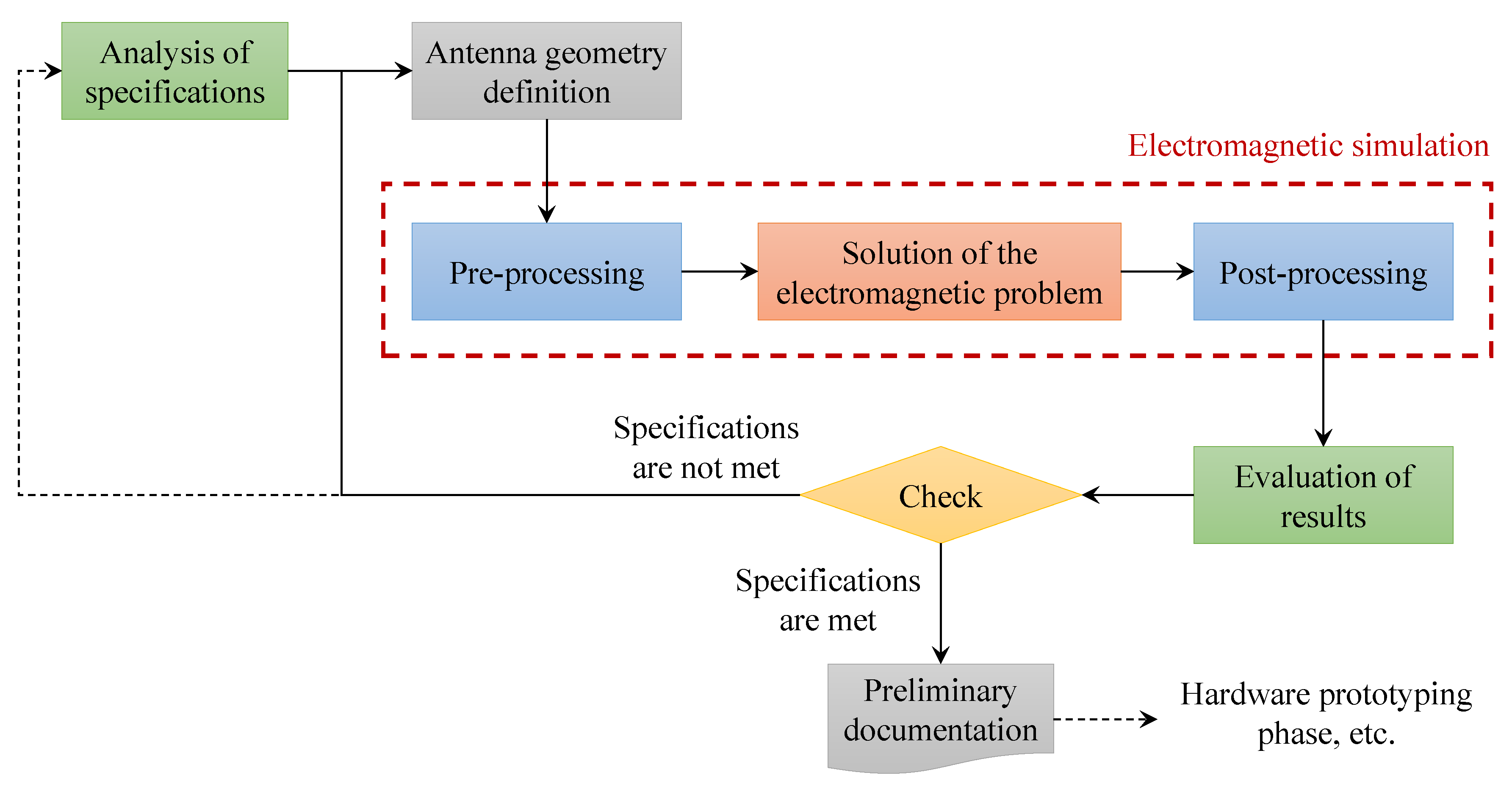
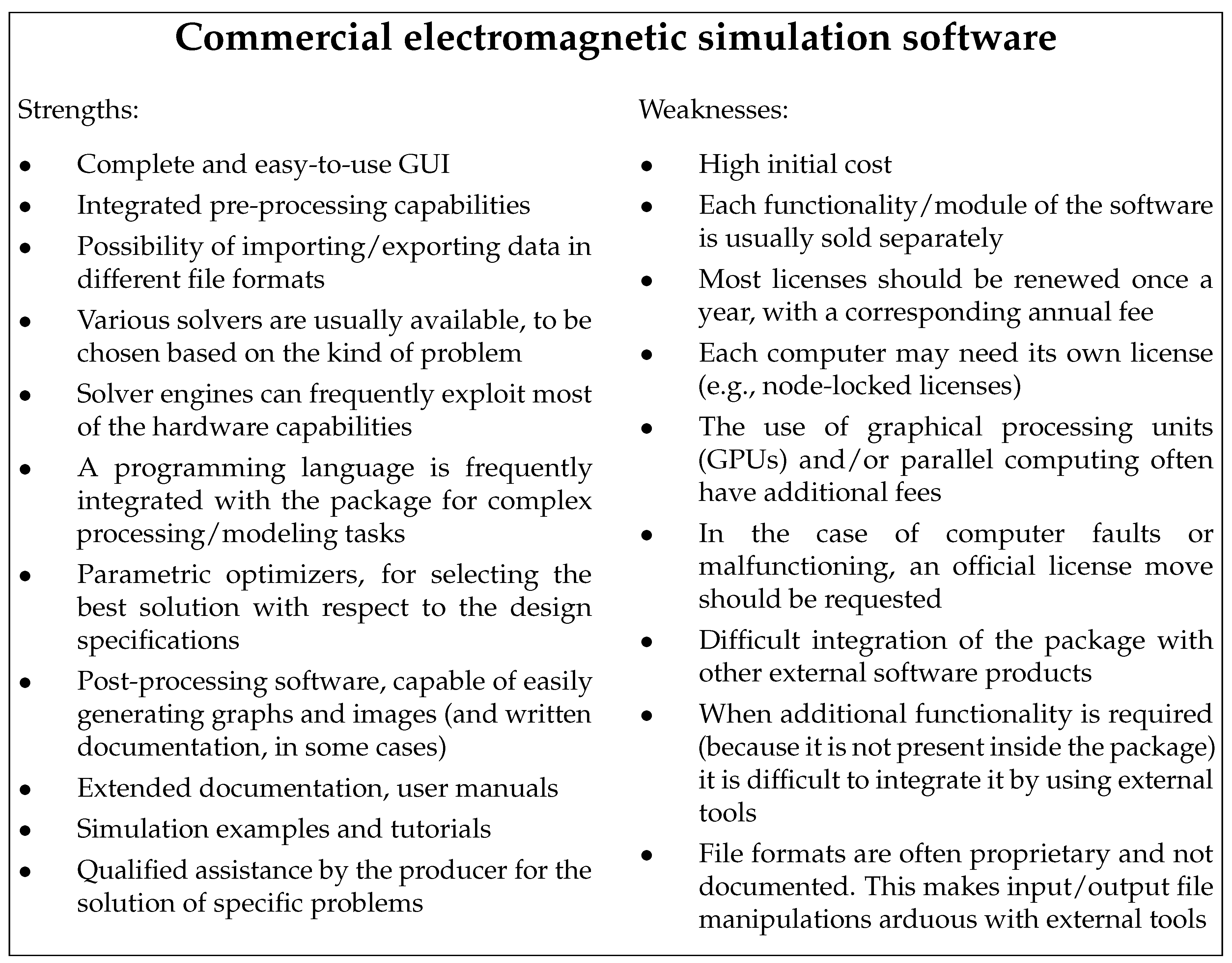
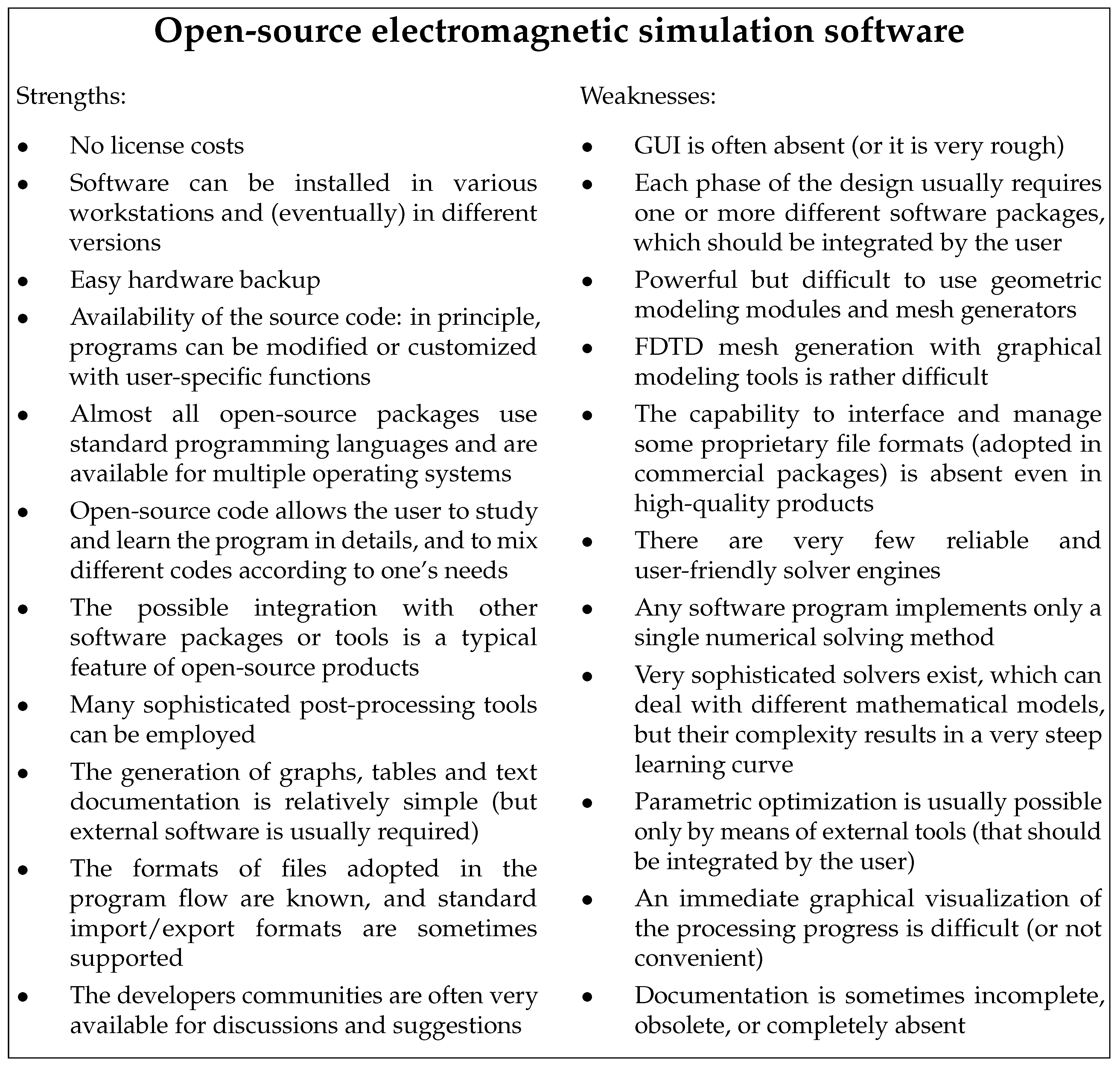
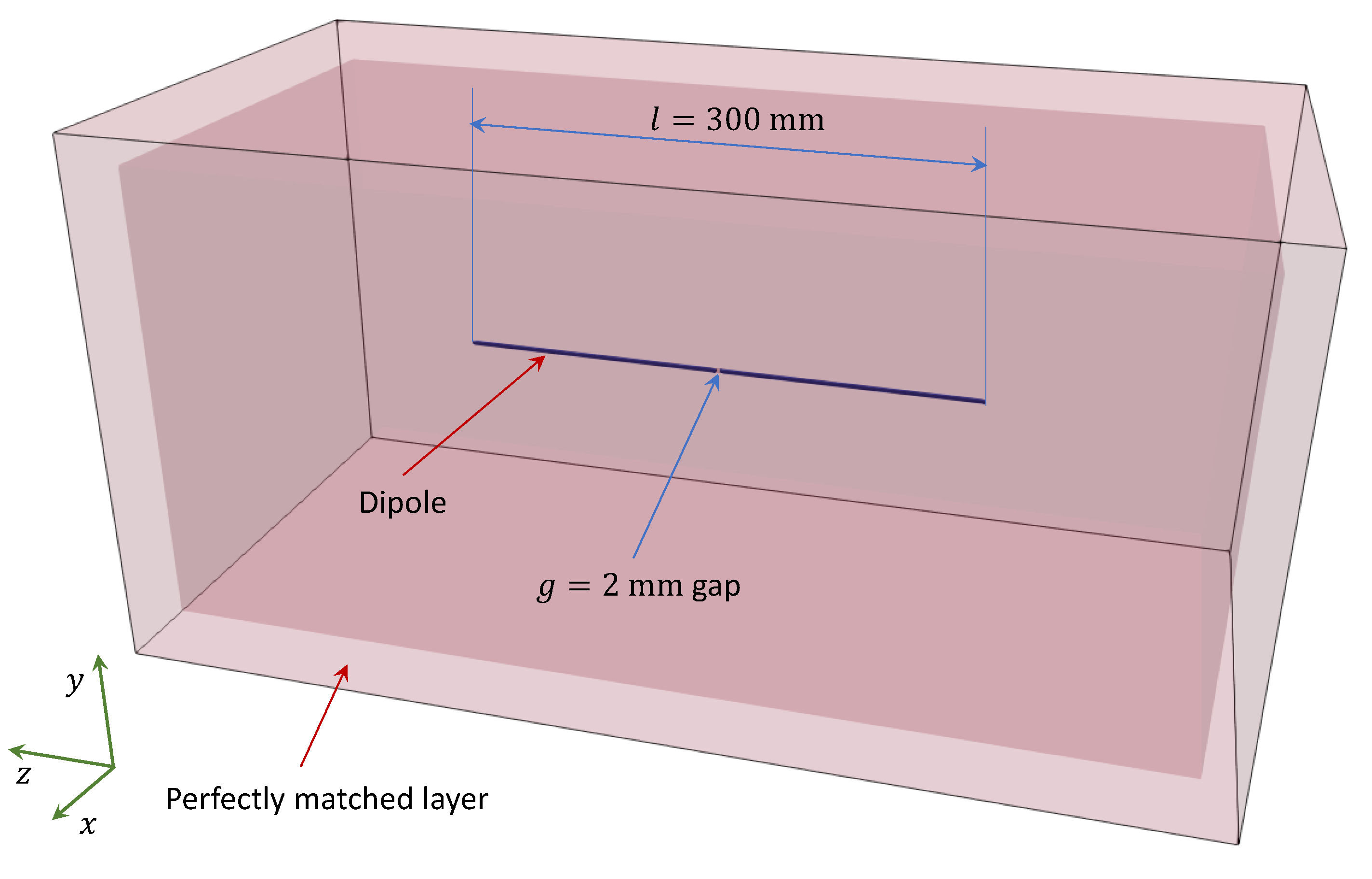
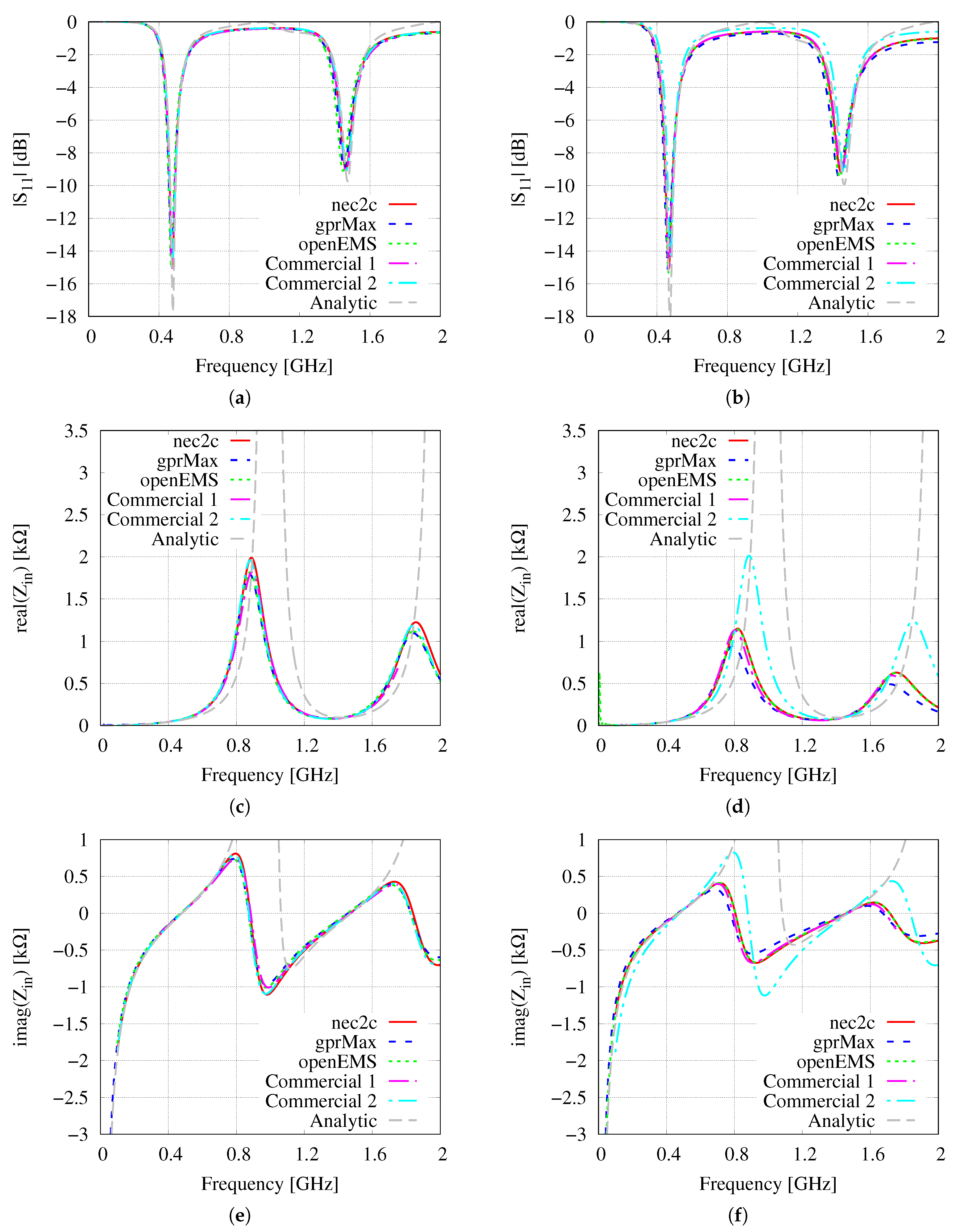
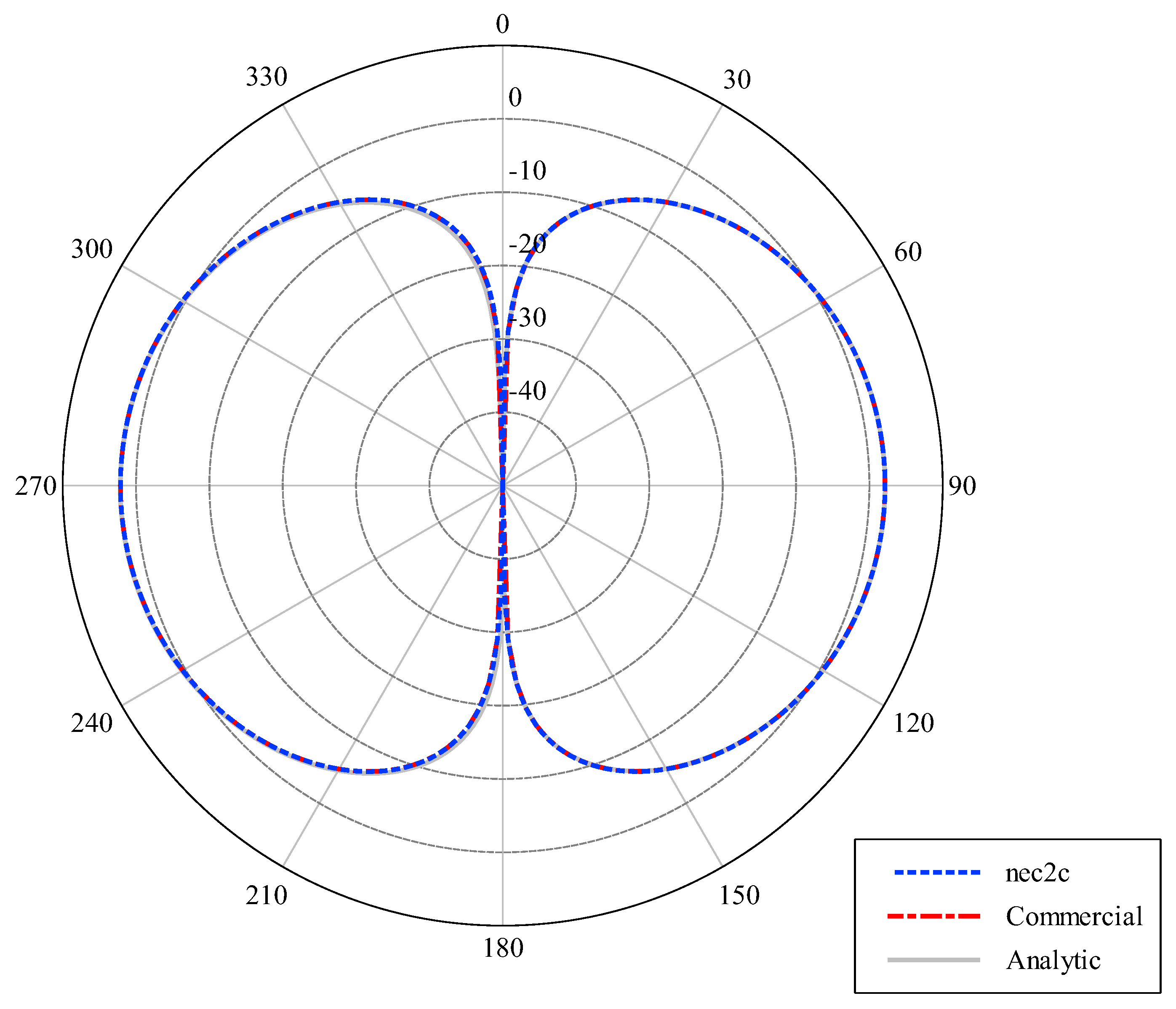
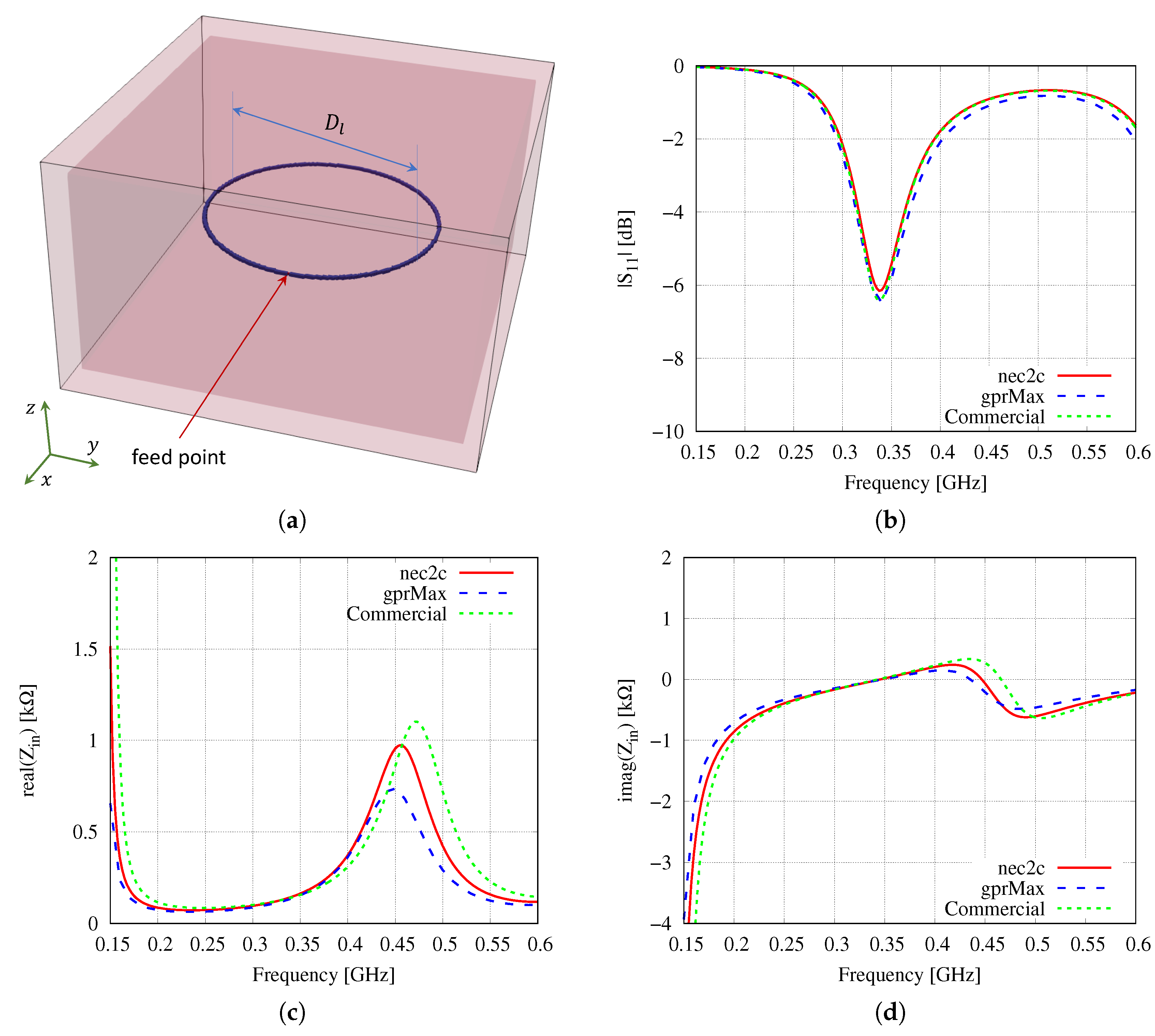
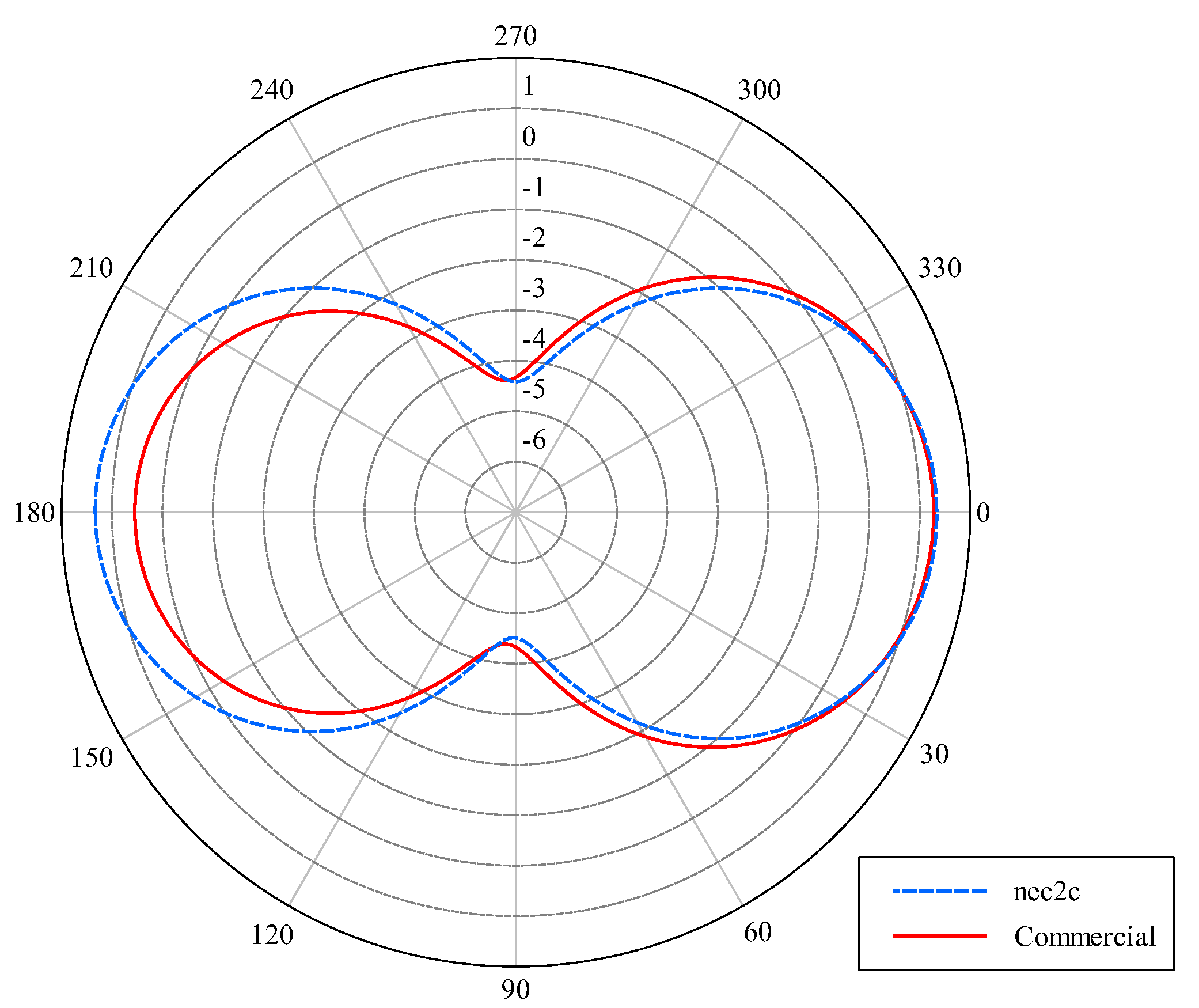
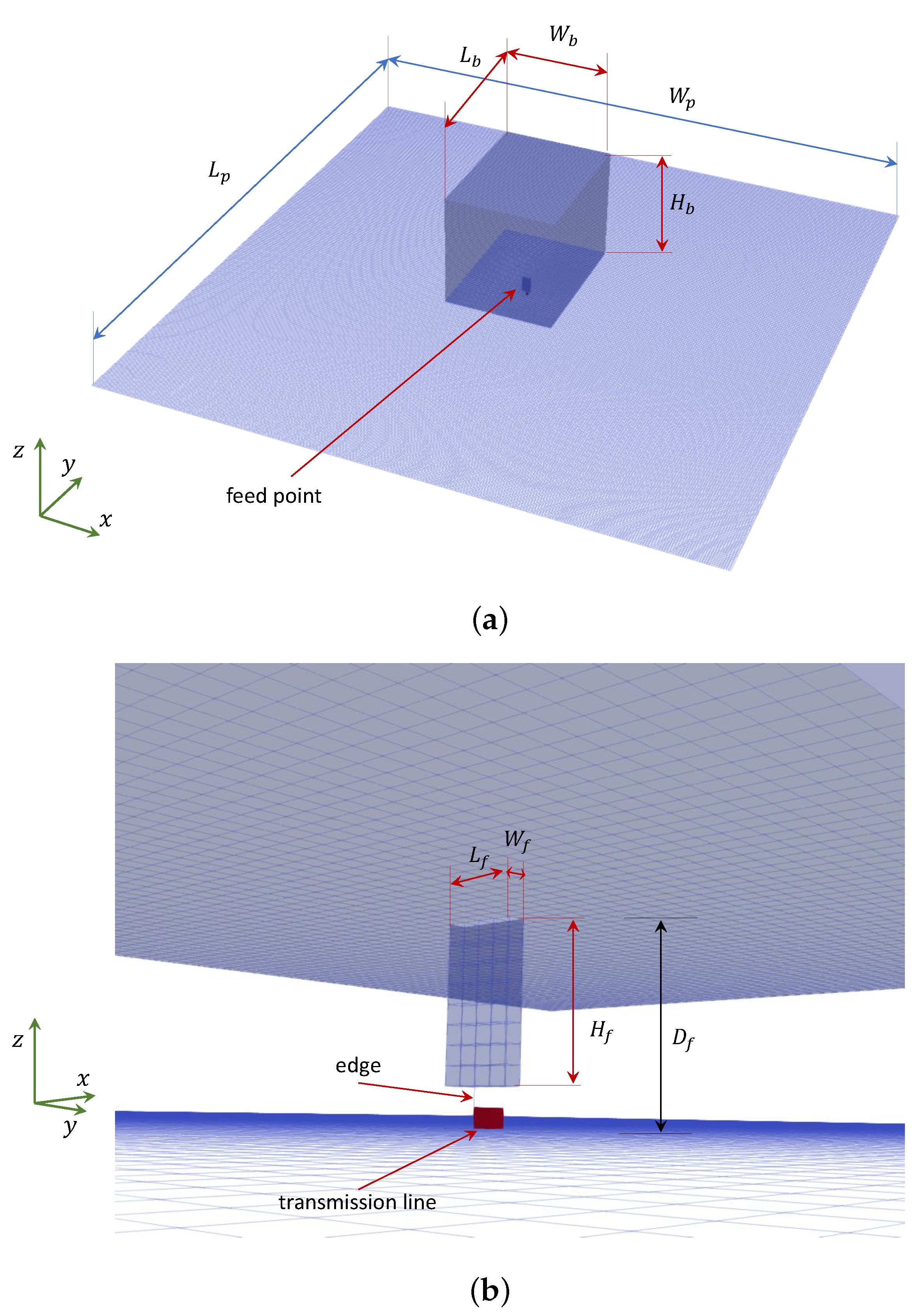
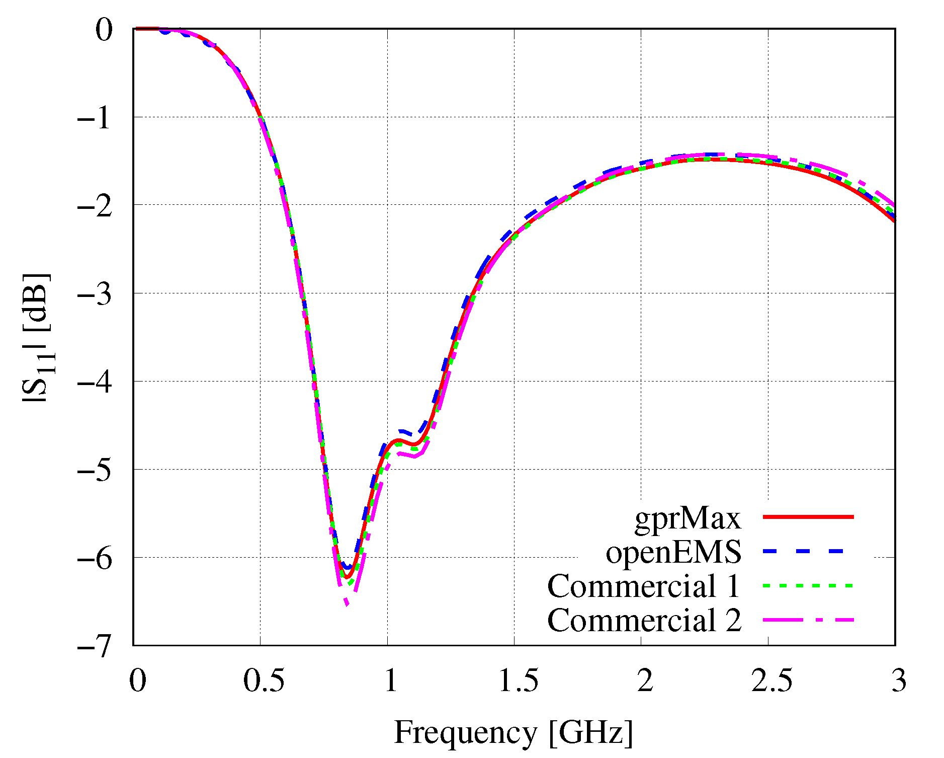
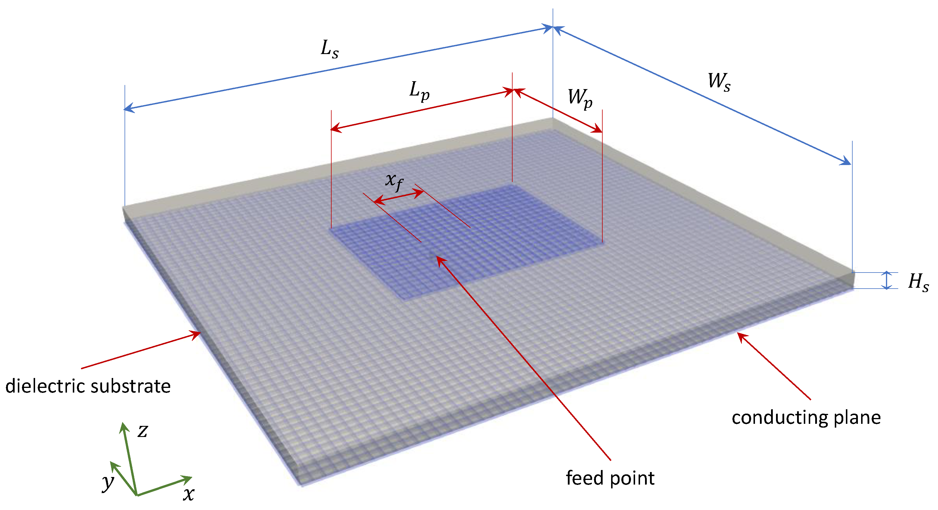
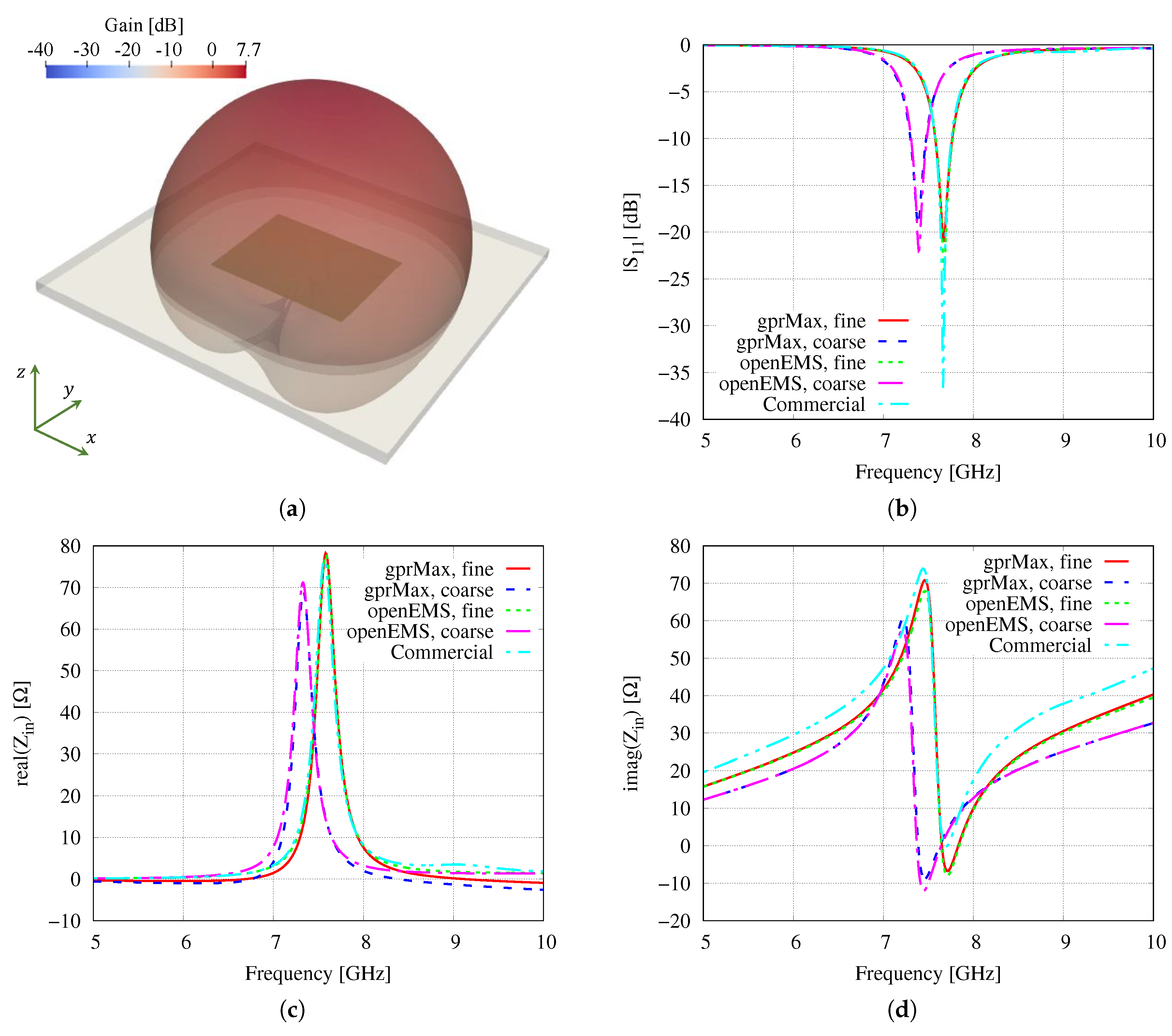
Table 1.
Error analysis between simulated and analytic results for the wire dipole antenna.
| Solver | [] | Error | [GHz] | Error | [GHz] | Error |
|---|---|---|---|---|---|---|
| nec2c | 0.143 | 0.478 | 0.005 | 1.469 | 0.004 | |
| gprMax | 0.207 | 0.473 | 0.014 | 1.456 | 0.012 | |
| openEMS | 0.255 | 0.472 | 0.018 | 1.453 | 0.015 | |
| Commercial 1 | 0.133 | 0.477 | 0.006 | 1.470 | 0.003 | |
| Commercial 2 | 0.129 | 0.479 | 0.003 | 1.472 | 0.002 | |
| Analytic | – | 0.480 | – | 1.475 | – |
Table 2.
Error analysis between simulated and analytic results for the cylindrical dipole antenna.
| Solver | [] | Error | [GHz] | Error | [GHz] | Error |
|---|---|---|---|---|---|---|
| nec2c | 0.225 | 0.470 | 0.009 | 1.461 | 0.0046 | |
| gprMax | 0.281 | 0.465 | 0.020 | 1.449 | 0.0130 | |
| openEMS | 0.252 | 0.468 | 0.014 | 1.453 | 0.0099 | |
| Commercial 1 | 0.219 | 0.472 | 0.007 | 1.466 | 0.0013 | |
| Commercial 2 | 0.149 | 0.477 | 0.005 | 1.467 | 0.0003 | |
| Analytic | – | 0.475 | – | 1.468 | – |
Table 3.
Specifications of the considered workstations.
| Workstation 1 | Workstation 2 | ||
|---|---|---|---|
| Type | i7-6700 CPU @ 3.40GHz | i9-7900X CPU @ 3.30GHz | |
| CPU | Configuration | cores = 4 threads = 8 | cores = 10 threads = 20 |
| Cache size (KB) | 8192 | 14,080 | |
| Memory | Size (GB) | 16 | 16 |
| Type | DDR4 2133 MHz (0.5 ns) | DDR4 2666 MHz (0.4 ns) |
Table 4.
Computational times related to the cylindrical dipole.
| Workstation 1 | |||||
|---|---|---|---|---|---|
| User Time,[s] | Sys. Time,[s] | [%] | Norm. Time,[s] | Elapsed Time [h:m:s] | |
| nec2c | 14.81 | 0.03 | 99 | 14.99 | 00:00:14.09 |
| gprMax | 5282.99 | 7.54 | 398 | 1329.28 | 00:22:06.00 |
| openEMS | 46,820.92 | 42.86 | 712 | 6581.99 | 01:49:41.00 |
| Workstation 2 | |||||
| User Time,[s] | Sys. Time,[s] | [%] | Norm. Time,[s] | Elapsed Time [h:m:s] | |
| nec2c | 12.86 | 0.03 | 99 | 13.02 | 00:00:12.09 |
| gprMax | 12,125.73 | 48.15 | 993 | 1225.97 | 00:20:25.08 |
| openEMS | 53,194.30 | 178.31 | 1296 | 4118.26 | 01:08:37.00 |
Table 5.
Computational times related to the patch antenna.
| Workstation 1 | |||||
|---|---|---|---|---|---|
| User Time,[s] | Sys. Time,[s] | [%] | Norm. Time,[s] | Elaps. Time,[h:m:s] | |
| gprMax | 810.45 | 1.85 | 397 | 204.61 | 00:03:24.00 |
| openEMS | 5820.55 | 9.52 | 710 | 821.14 | 00:13:41.01 |
| Workstation 2 | |||||
| User Time,[s] | Sys. Time,[s] | [%] | Norm. Time,[s] | Elaps. Time,[h:m:s] | |
| gprMax | 1764.18 | 10.77 | 987 | 179.83 | 00:02:59.07 |
| openEMS | 6724.96 | 34.54 | 1287 | 525.21 | 00:08:44.01 |
Table 6.
Computational times related to the box-plate antenna.
| Workstation 1 | |||||
|---|---|---|---|---|---|
| User Time,[s] | Sys. Time,[s] | [%] | Norm. Time,[s] | Elaps. Time,[h:m:s] | |
| gprMax | 109,012.22 | 20.42 | 399 | 27,326.48 | 07:34:47.00 |
| openEMS | 712,364.29 | 149.83 | 720 | 98,960.29 | 27:28:25.00 |
| Workstation 2 | |||||
| User Time,[s] | Sys. Time,[s] | [%] | Norm. Time,[s] | Elaps. Time,[h:m:s] | |
| gprMax | 244,765.11 | 119.14 | 983 | 24,911.93 | 06:55:06.00 |
| openEMS | 814,999.02 | 622.13 | 1481 | 55,072.33 | 15:17:48.08 |
Table 7.
Computational times related to the loop antenna.
| Workstation 1 | |||||
|---|---|---|---|---|---|
| User Time,[s] | Sys. Time,[s] | [%] | Norm. Time,[s] | Elaps. Time,[h:m:s] | |
| nec2c | 1332.38 | 7.57 | 99 | 1353.48 | 00:22:25.00 |
| gprMax | 8509.15 | 7.81 | 398 | 2140.03 | 00:35:34.08 |
| Workstation 2 | |||||
| User Time,[s] | Sys. Time,[s] | [%] | Norm. Time,[s] | Elaps. Time,[h:m:s] | |
| nec2c | 1181.29 | 6.10 | 99 | 1199.38 | 00:19:48.07 |
| gprMax | 20,961.51 | 50.93 | 995 | 2111.80 | 00:35:10.05 |
Table 8.
Parallelization capabilities of the considered open-source software packages for electromagnetic simulation.
Table 8.
Parallelization capabilities of the considered open-source software packages for electromagnetic simulation.
| Solver | Method | Parallelization Capabilities |
|---|---|---|
| nec2c | MoM | Single-CPU Single-thread |
| xnec2c | MoM | Single-CPU Multi-thread |
| gprMax | FDTD | openMP, MPI, CUDA |
| openEMS | FDTD | MPI, SSE |
© 2019 by the authors. Licensee MDPI, Basel, Switzerland. This article is an open access article distributed under the terms and conditions of the Creative Commons Attribution (CC BY) license (http://creativecommons.org/licenses/by/4.0/).
Share and Cite
MDPI and ACS Style
Fedeli, A.; Montecucco, C.; Gragnani, G.L. Open-Source Software for Electromagnetic Scattering Simulation: The Case of Antenna Design. Electronics 2019, 8, 1506. https://0-doi-org.brum.beds.ac.uk/10.3390/electronics8121506
AMA Style
Fedeli A, Montecucco C, Gragnani GL. Open-Source Software for Electromagnetic Scattering Simulation: The Case of Antenna Design. Electronics. 2019; 8(12):1506. https://0-doi-org.brum.beds.ac.uk/10.3390/electronics8121506
Chicago/Turabian StyleFedeli, Alessandro, Claudio Montecucco, and Gian Luigi Gragnani. 2019. "Open-Source Software for Electromagnetic Scattering Simulation: The Case of Antenna Design" Electronics 8, no. 12: 1506. https://0-doi-org.brum.beds.ac.uk/10.3390/electronics8121506
Note that from the first issue of 2016, this journal uses article numbers instead of page numbers. See further details here.