A Forecasting Model for Economic Growth and CO₂ Emission Based on Industry 4.0 Political Policy under the Government Power: Adapting a Second-Order Autoregressive-SEM

Abstract

This research aims to forecast future economic and environmental growth for the next 16 years (2020–2035) according to the government’s strategic framework by applying the second order autoregressive-structural equation model (second order autoregressive-SEM). The model is validated by various measures, fits with the best model standards, meets all criteria of the goodness of fit, and is absent from any issues of heteroskedasticity, multicollinearity, autocorrelation, and non-normality. The proposed model is very distinct from other alternatives in that it produces the optimal outcome. Its mean absolute percentage error (MAPE) is 1.02% while the root mean square error (RMSE) is 1.51%. A comparison of the above results is carried out to compare the same values from other models, namely the regression linear model (ML model), back propagation neural network (BP model), artificial neural natural model (ANN model), gray model, and the autoregressive integrated moving average model (ARIMA model). The second order autoregressive-SEM is a model that is appropriate for long-term forecasting (2020–2035), and accounts for the specifics of the Thai government strategy set under the Industry 4.0 policy framework. The results of the long-term analysis indicate that the current political policy $(Politi)$ will result in continuous economic growth, where the gross national product (GNP) growth rate will climb up to 6.45% per annum by 2035, while the environment is being negatively affected. The study predicts that CO₂ emissions will rise up to 97.52 Mt CO₂ Eq. (2035). The forecasting model also reflects that the economy factor has an adjustment ability to equilibrium stronger than that of the environment factor; further, it shows that the relationship between the factors is causal. In addition, the political policy $(Politi)$, economy $(Econ)$, and environment $(Environ)$ factors are found to have both direct and indirect effects. As to the results, this study illustrates that the Industry 4.0 policy is still inefficient, as the carbon dioxide emissions are projected to be higher than the threshold for environment hazards and disasters which set to the limit of 80 Mt CO₂ Eq. by 2035. The effect of such policy will put the environment at risk, and the government must take immediate action to respond to this urgency. Thus, the second order autoregressive-SEM model remains a significant model embedded with the adjustment ability to equilibrium and the applicability for various contexts in different sectors. This introduced model is a vital tool for assisting the national government to create policy that is effective and sustainable, and lead to positive development of the nation. This second order autoregressive-SEM model can be used as a resource for the management of both public policy and private enterprise.

1. Introduction

The Thai government established a national strategy in 1990, which is still in effect, aimed at creating and maintaining sustainability. The government has also made an effort to promote the Industry 4.0 policy, with the aim of enhancing the development of the Thai economy and increasing the growth rate of the gross national product (GNP). In fact, Thailand has been supporting all sectors, especially industrial sector, in order to ensure their development and growth. Such promotion and supportive actions are provided through both aggressive and receptive strategies in various dimensions, in both the short-term (1–5 years) and long-term (10–20 years) [1,2]. In the short run, immediate aggressive and receptive policies have been put into place to help generate a national revenue [3]. These include measures in the industries of transportation, textiles, iron and steel, and other industrial products that are exclusively outside of the agricultural sector. In addition, with respect to the long run, the government has implemented a number of different strategies, such as promoting exports and diversifying products for export, encouraging foreign direct investment, developing the tourism industry, improving labor skills for heavy industry, expanding local markets for foreign investors, adjusting the tax basis, and developing large industries of the government among many others [4].

The implementation of such policies aims to create economic growth, leading to an increasing rate of GNP growth. In addition, Thailand’s imports seem to be declining as the country expands its production base, enabling Thai industry to support internal consumption and domestic needs. In addition, the government has focused on the export of important products and sought to expand overseas export opportunities [5,6]. For this reason, the Thai economy is being continuously developed, and managing to attract investment from various countries into heavy industry, generating national revenue. In fact, the Thai government has formulated a long-term strategy for economic and social development that focuses on various fields across all sectors, including increasing employment opportunity, providing services related to health and illness, strengthening social security and imposing greater consumer protection [7]. These are positive developments that support economic and social growth—however, there are negative outcomes as well. For example, energy consumption and greenhouse gas emissions are found to be rising continuously (reference), especially in the industrial sector where these negative environmental trends date back to at least 1990. In particular, it has been found that increased production activity in Thailand has led to higher CO₂ emissions in all sectors, including both industrial sectors and non-industrial sectors, resulting in an increase in greenhouse gases of up to 78.25% (2018) [8,9]. Evidence suggests that the implementation of policies by the Thai government has led to economic and societal development, but that this has come at the cost of environmental deterioration, in part because the government policy suffered from a lack of clear environmental assessment tools [10,11]. This lack of available tools needed to support formulation of national policies causing many errors in planning process [12,13].

Industry 4.0-based government policy has had a positive effect on the Thai economy. However, if the policy is meant to create sustainability, then both social and environmental aspects should be given a boost at the same time, illustrating the efficiency of the appropriate government operation [14,15]. This research, unfortunately, shows that Thailand still lacks important tools that are necessary for formulating policies. Hence, the researchers have attempted to develop a tool to facilitate in government policy formulation and planning by utilizing the second order autoregressive-SEM model. In addition to this modelling, optimization of the model for forecasting has been undertaken in an effort to examine the efficiency of the Industry 4.0 policy. Such forecasting includes predicting GNP and CO₂ emission for the long term (2019–2035), which is a difficult and challenging task. This model also stands out from other existing models because of its suitability for application in different sectors.

2. Literature Review

This part offers a discussion and review of the existing literature and revisits relevant studies for a deeper understanding of the relationships and connections between factors affecting the subject of this paper. There have been a number of studies in this area of research, meaning that this paper is well-furnished with existing resources. Among the many studies, Oh and Shin [16] investigated the future cash flow forecast information given by accounting and financial analysts of Korean listed firms for the years 2011 to 2015. Their findings indicate that the existence of an information-rich environment can reduce information asymmetry between the manager and the investor. He and Yin [17] examined the influence of a firm’s deviant strategy on analysts’ earnings forecasts while exploring the topic of a firm’s information transparency and environmental uncertainty in terms of information asymmetry. They discovered that such a strategy has an effect on analysts’ earnings forecasts. Meanwhile, Dong et al. [18] evaluated the relationship between outdoor air pollutants (PM₁₀), sulfur dioxide (SO₂) and nitrogen dioxide (NO₂), and mortality in China, and discovered a significant relationship between PM₁₀ and NO₂ levels and mortality.

In addition to the investigation of these factor relationships, a number of studies have put forward different models to facilitate the work of forecasting. For example, Xu and Ren [19] proposed a hybrid model based on an echo state network (ESN) and an improved particle swarm optimization (IPSO) algorithm to study air pollution in Beijing, while providing a forecasting method for particulate matter (PM_2.5). To this extent, their proposed model outperforms compared to comparative models. Zu and Ren [20] also proposed a supplementary leaky integrator echo state network (SLI-ESN) for accurate forecasting the PM_2.5 time series. This model has been validated and its prediction accuracy proven. The model demonstrates outstanding performance and excellence in application, as shown by the study’s finding. Tsui et al. [21] carried out a study to forecast airport passenger traffic for Hong Kong airport through 2015 while estimating its future growth trend by deploying the Box-Jenkins Seasonal ARIMA (SARIMA) model and the ARIMAX model, which projected Hong Kong airport’s future passenger traffic to grow steadily, but at fluctuating rates. Moreover, Mahajan et al. [22] developed an historical data-based method to forecast PM_2.5 in Taiwan for 132 stations. The method was able to produce forecasting with error rates as low as 0.16 µg/m³. In addition to this outcome, 90% of the monitoring stations have subsequently been found to be under 1.5 µg/m³ error. Huang et al. [23] developed a novel forecasting method to predict multi-step short-term wind speed by adapting the ensemble empirical mode decomposition (EEMD). It has further been shown that this study’s developed model, as a result, can actually enhance the capacity of wind speed. Among many other potential models, Wu and Lin [24] conducted a study with development of a hybrid wind speed forecasting model to better improve prediction performance by incorporating variational mode decomposition (VMD). The result of the study showed that the hybrid model has a greater accuracy in forecasting ultra-short-term (15 min) and short-term (1 h) wind speeds. Also, a systematic design of a multistage artificial neural network-based short-term load forecaster was developed to improve forecasting performance. With that, they found an error in forecasting, carried out by Methaprayoon et al. [25]. Fan and Hyndman [26] forecasted demand for electricity in the Australian National Electricity Market, saying that there should be different metrics and criteria for adaption of this forecast. As for Ramos and Oliveira [27], they produced a cross-validation procedure to determine appropriate models: the autoregressive integrated moving average model and state space model. Based on their study, such cross-validation procedure has been used to support accurate forecasting and accuracy enhancement.

When it comes to forecasting energy consumption, a number of research studies have been conducted to investigate and estimate possible trends by proposing various models. Shi et al. [28] improved wind power forecasting by developing a hybrid model incorporating with other single models, and their study outcome presents the validity of the hybrid as having greater application in very-short term forecasting of wind power. Hyndman and Fan [20] forecasted the density of long-term peak electricity demand by proposing a new and systematic methodology, and the model outperforms others, as shown by the results of the study. In other research, Chen et al. [29] developed a novel least-squares support vector regression with a Google (LSSVR-G) model to predict the power output from various sources in Taiwan, including renewable power, thermal power and nuclear power. The discussion of this study indicated that the proposed LSSVR-G model performs better than any previously studied models with respect to accuracy and stability. In another study, Lu et al. [30] aimed to ameliorate the ultra-short-term accuracy of wind power forecasting. This led to the proposal of a novel hybrid wind power time series prediction model, adapting ensemble empirical mode decomposition-permutation entropy (EEMD-PE), the least squares support vector machine model (LSSVM), and gravitational search algorithm (GSA). There is no doubt that the proposed model outperforms the alternatives. Guan et al. [31] contributed to the field of study by proposing an advanced load forecast (ALF) system with hierarchical forecasting capability, and it turned the system into a potential tool for distribution system load forecasting. Xie, Hong and Stroud [32] predicted long-term retail energy requirements by doing a regression analysis and survival analysis. In this study, they uncovered the effectiveness of the approach, and demonstrated the superiority of the model to other models. Furthermore, Sun et al. [33] set out to apply multi-step wind speed forecasting (WSF) to the development of a novel forecasting strategy. With such application of WSF, they illustrated the effectiveness of the proposed model, ensemble empirical mode decomposition (EEMD)/variational mode decomposition (VMD)-hybrid backtracking search optimization algorithm (HBSA)-double activations through weighted coefficient (DAWNN).

In Lithuania, Bobinaite et al. [34] examined the linkage between economic growth (GDP) and renewable energy consumption (RES) by employing unit root, co-integration and Granger causality tests. Here, they have found a unidirectional relationship running from RES gross inland consumption to real GDP in the short run. The same relationship was also analyzed by Soava et al. [35] in the EU with the application of panel data techniques. As for their finding, the influence of renewable energy consumption on economic growth was found to be positive. The same result has also been supported by Lots [36], and Pao and Fu [37]. Rafiq and Salim [38] extended the same study to six emerging economies of Asia by using co-integration and vector error correction modeling. The same impact was found vary from country to country. On a bigger scale, the same linkage was studied by Chontanawat et al. [39] with the use of a causality test, along with an illustration of the prevalent causality of developed OECD countries than any other developing non-OECD countries. However, Pao and Fu added non-renewable energy into the relationship in the Brazilian context with the use of the co-integration test and found the linkage of the additional variable on primary energy consumption to be insignificant. In the same case of the EU context, Sterpu et al. [40] further addressed the investigation into the causal relationship between per capita greenhouse gas (GHG) emissions, gross domestic product, gross inland energy consumption, and renewable energy consumption by testing the environmental Kuznets curve (EKC) hypothesis via a panel co-integration approach. Their study indicates that there will be a rise of GHGs when gross energy consumption rises. In contrast, GHGs will be reduced when renewable energy consumption increases. In India, Jiang, Yang and Li [41] used metabolic grey model (MGM), autoregressive integrated moving average (ARIMA), MGM-ARIMA, and back propagation neural network (BP) in their work to estimate energy demand. The study indicates a 5% growth in energy consumption from 2017 to 2030. Wang, Zhan and Li [42] investigated and forecast energy demand in Middle Africa for 14 years (2017–2030). Their forecast projects a growth rate of 5.37% in energy demand. At around the same time, Ma et al. [43] adopted the linear (metabolic grey model), nonlinear (non-linear grey model), and combined (metabolic grey model-autoregressive integrated moving average model) models to predict South Africa’s coal consumption for the years 2017 to 2030. The forecasting outcome of this study predicts a downward trend for these years (2017 to 2030), with a resulting drop of 1.9% per year, on average. Boyd et al. [44] optimized the ARIMA model to forecast daily influent to wastewater treatment plants (WWTPs). In this study, it was shown that the ARIMA model can actually produce more reliable daily influent forecasts, which can be further extended to include municipal and rural WWTPs, with enough information. In Sweden, Al-Douri et al. [45] generated a novel two-level multi-objective genetic algorithm (GA) to develop forecasting data for fans used in road tunnels by the Swedish Transport Administration (Trafikverket). The algorithm developed in this study demonstrated better performance than alternative models. In South Korea, Alsharif et al. [46] attempted to forecast daily and monthly solar radiation for 37 years (1981–2017) by developing a seasonal auto-regressive integrated moving average (SARIMA) model. The daily solar radiation was handled by the ARIMA model, while the monthly solar radiation was handled by the seasonal ARIMA; the average monthly solar radiation projected was in the range of 176 to 377 Wh/m².

There have also been studies aimed at improving forecasting capacity and accuracy. Liu et al. [47] deployed fuzzy combination weights, the empirical mode decomposition process, support vector machine and the Kalman filtering process, to develop a hybrid forecasting model capable of outperforming in forecasting and producing accurate results. Lee and Lin [48] attempted to develop an SVR-based load forecasting model deploying quantum behaviors and the TS algorithm along with vector regression for forecasting enhancement. Their study demonstrated that the proposed model is superior to other alternatives. Cai et al. [49] collaborated to develop a new hybrid model, integrating support vector regression (SVR), artificial bee colony (ABC) algorithm (ABC-SVR), and seasonal autoregressive integrated moving average (SARIMA) models. This hybrid model is expected to produce more accuracy in forecasting compared to other models. Lastly, Liu et al. [50] came up with a practical methodology for the use of quantile regression in order to support the probabilistic load forecasts, and that method was found by the authors of the study to be effective and efficient.

Based on a review of relevant studies, it can be concluded that research in this area differs from other existing studies, in that the second order autoregressive-SEM is a model that comes with high validity and the ability to close research gaps left by other studies. In fact, this research uses advanced statistics and detailed research procedures, enabling optimal results for determining long-term national policies to be generated while reducing potential errors. In addition, this research offers a newly developed model, making it different from models of the past. Its unique features include the adjustment ability to equilibrium, and applicability to various sectors. It is also important to understand that some previous studies did not consider certain issues, such as heteroskedasticity, multicollinearity, and autocorrelation in their analysis. Yet, this research ensures that those issues were carefully taken into account through in-depth analysis. Moreover, these studies have left some gaps, in that they did not consider the analysis of stationarity and co-integration of the model’s variables. Therefore, this piece of research attempts to bridge those gaps in order to produce accurate outcomes of the research, and that ensures the absence of the model’s spuriousness. Also, the exogenous variables were carefully selected for this particular model. The research applies the linear structural relations (LISREL) while deploying time series data from 1990 to 2018 for the prediction of gross national product (GNP) growth rate and CO₂ emissions during 2020 to 2035. The research flow can be explained as shown in Figure 1.

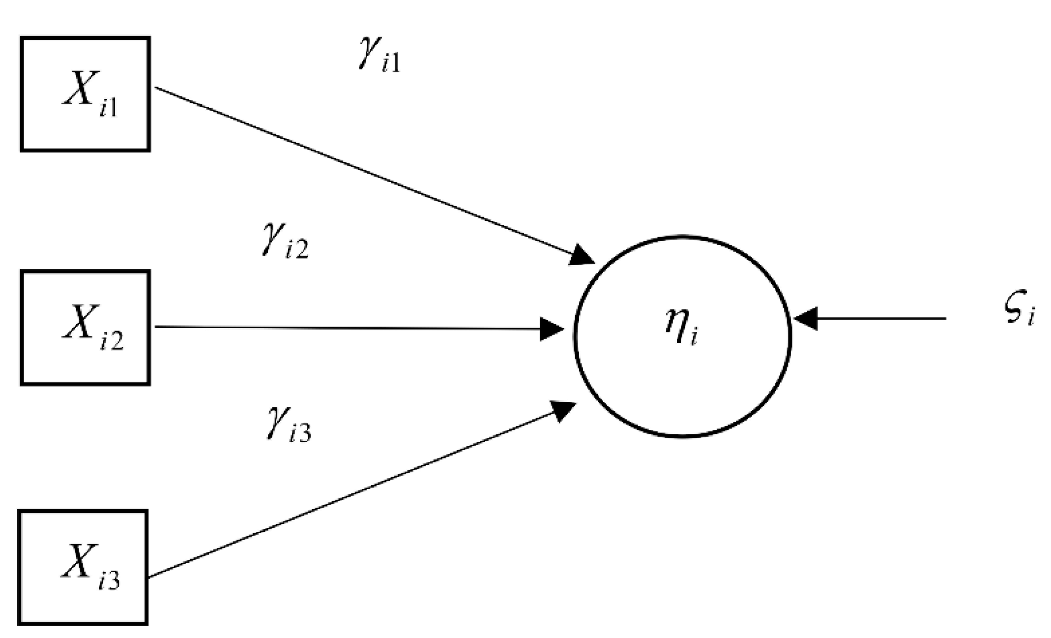
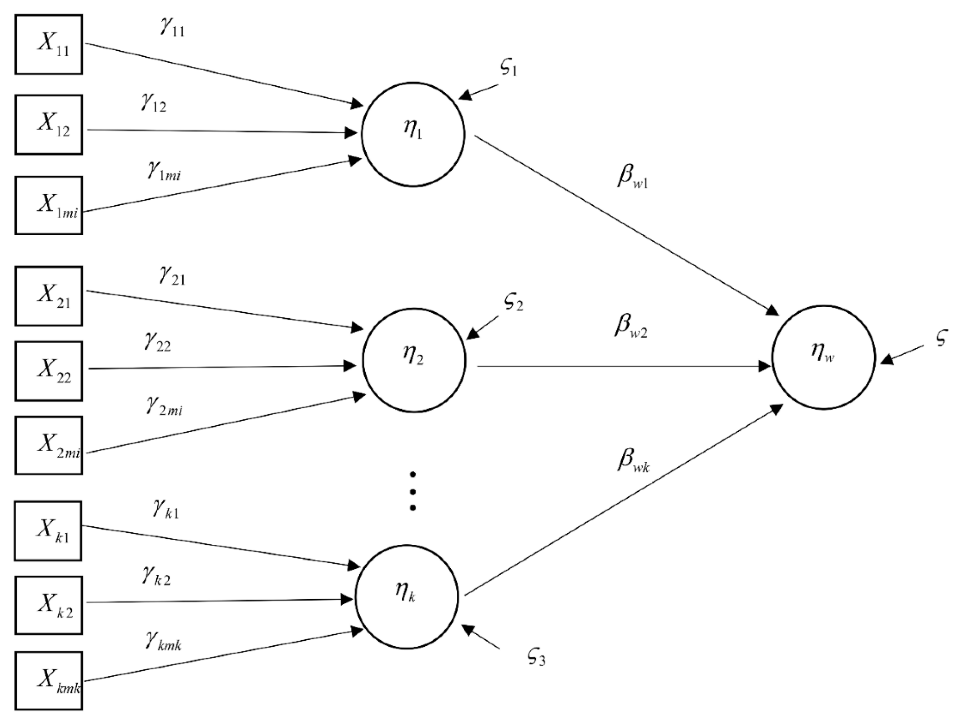
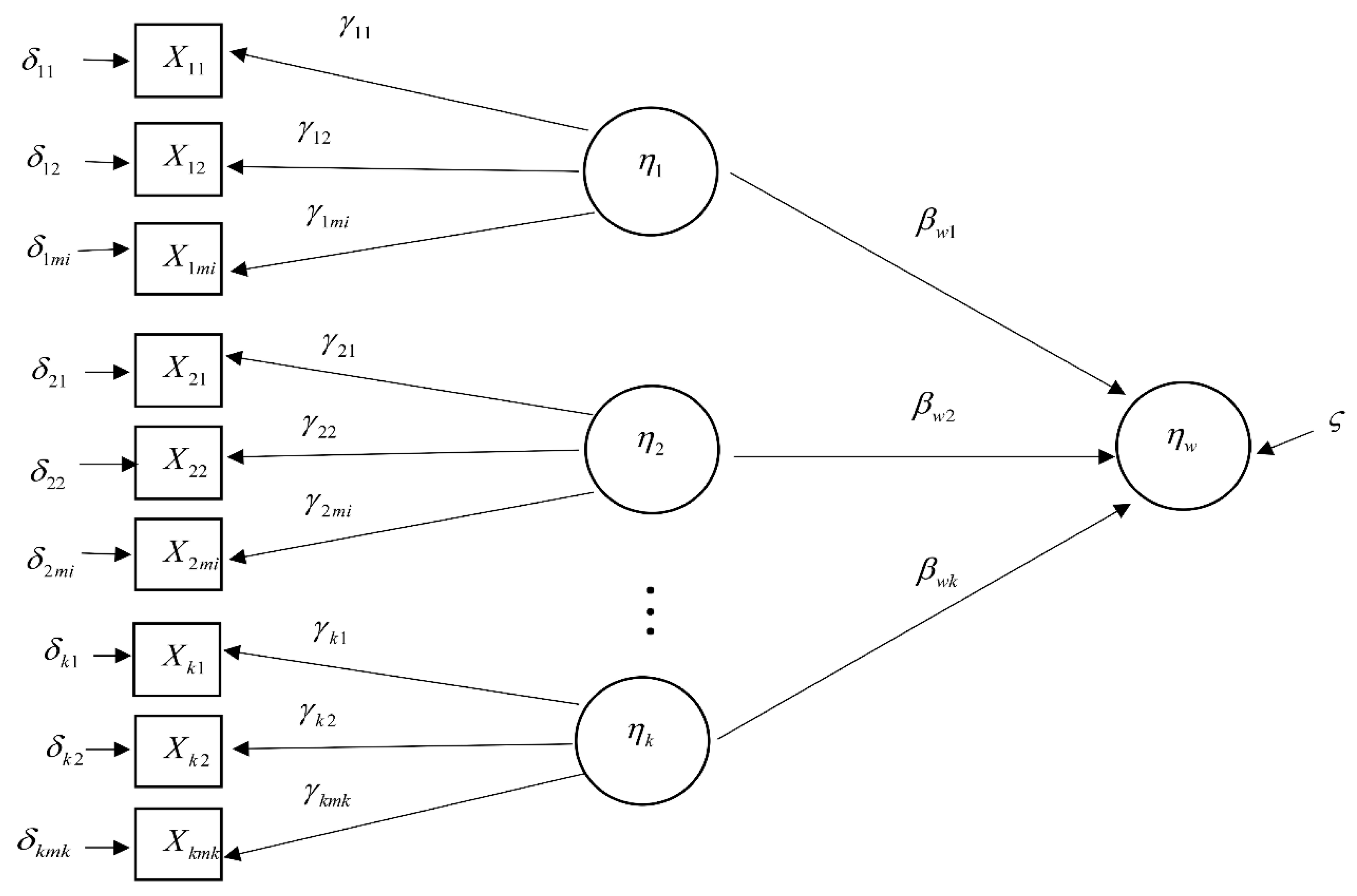
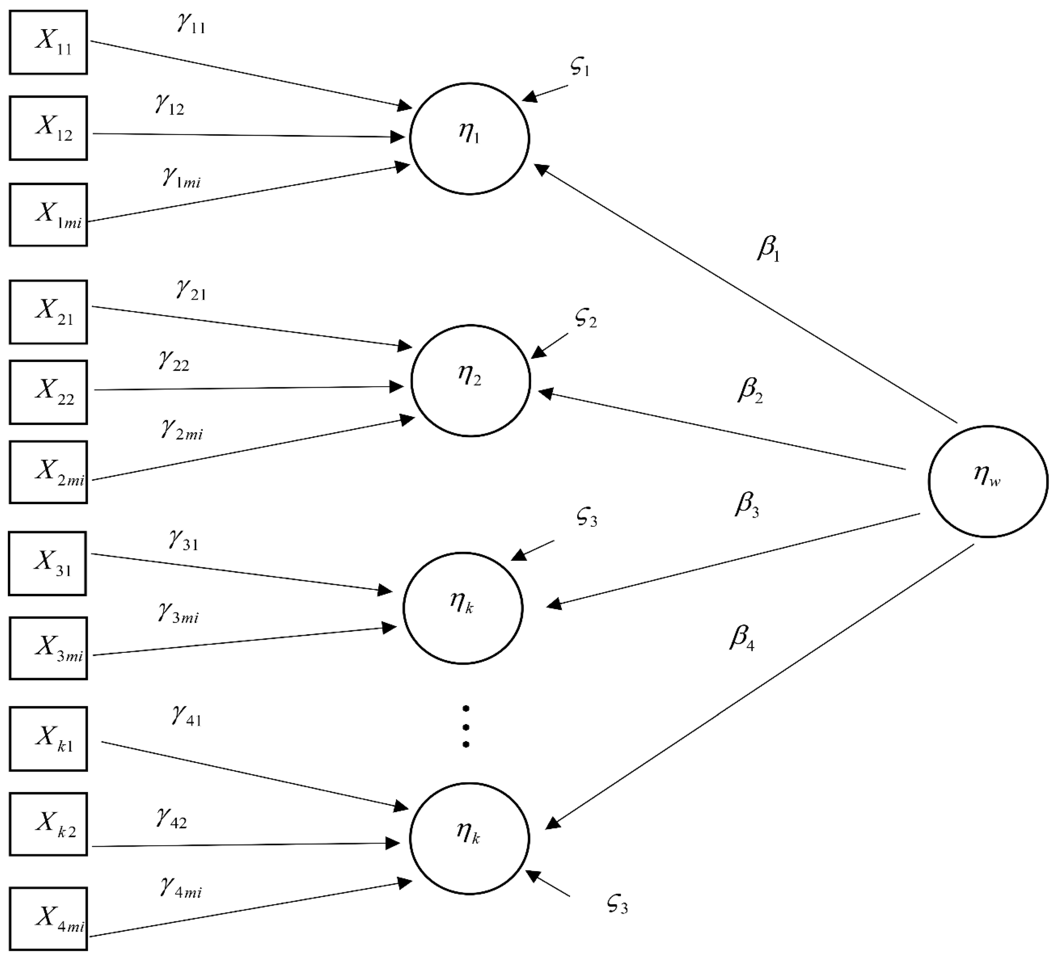
• Select variables for use in constructing the second order autoregressive-SEM, in which objectives have been specified by the government in the national strategy. The latent variables are political policy $(Politi)$, the economy $(Econ)$, and the environment $(Environ)$, while the observed variables are national income $(NI)$, urbanization rate $(Ur)$, industrial structure $(Si)$, net exports $(E-I)$, foreign investment $(FI)$, foreign tourism $(Ft)$, employment $(Em)$, government investment $(Gi)$, government subsidy $(Gs)$, technology investment $(Te)$, energy consumption $(Ec)$, energy intensity $(EI)$, and carbon dioxide emission $(C{O}_2)$. The reason of considering the observed variables is to formulate a national objective of Thailand in terms of political policy $(Politi)$, which emphasizes three main indicators: government investment $(Gi)$, government subsidy $(Gs)$, and technology investment $(Te)$. The indicators in economy $(Econ)$ are inclusive of national income $(NI)$, urbanization rate $(Ur)$, industrial structure $(Si)$, net exports $(E-I)$, foreign investment $(FI)$, foreign tourism $(Ft)$, and employment $(Em)$, while the indicators in environment $(Environ)$ are energy consumption $(Ec)$, energy intensity $(EI)$, and carbon dioxide emissions $(C{O}_2)$.
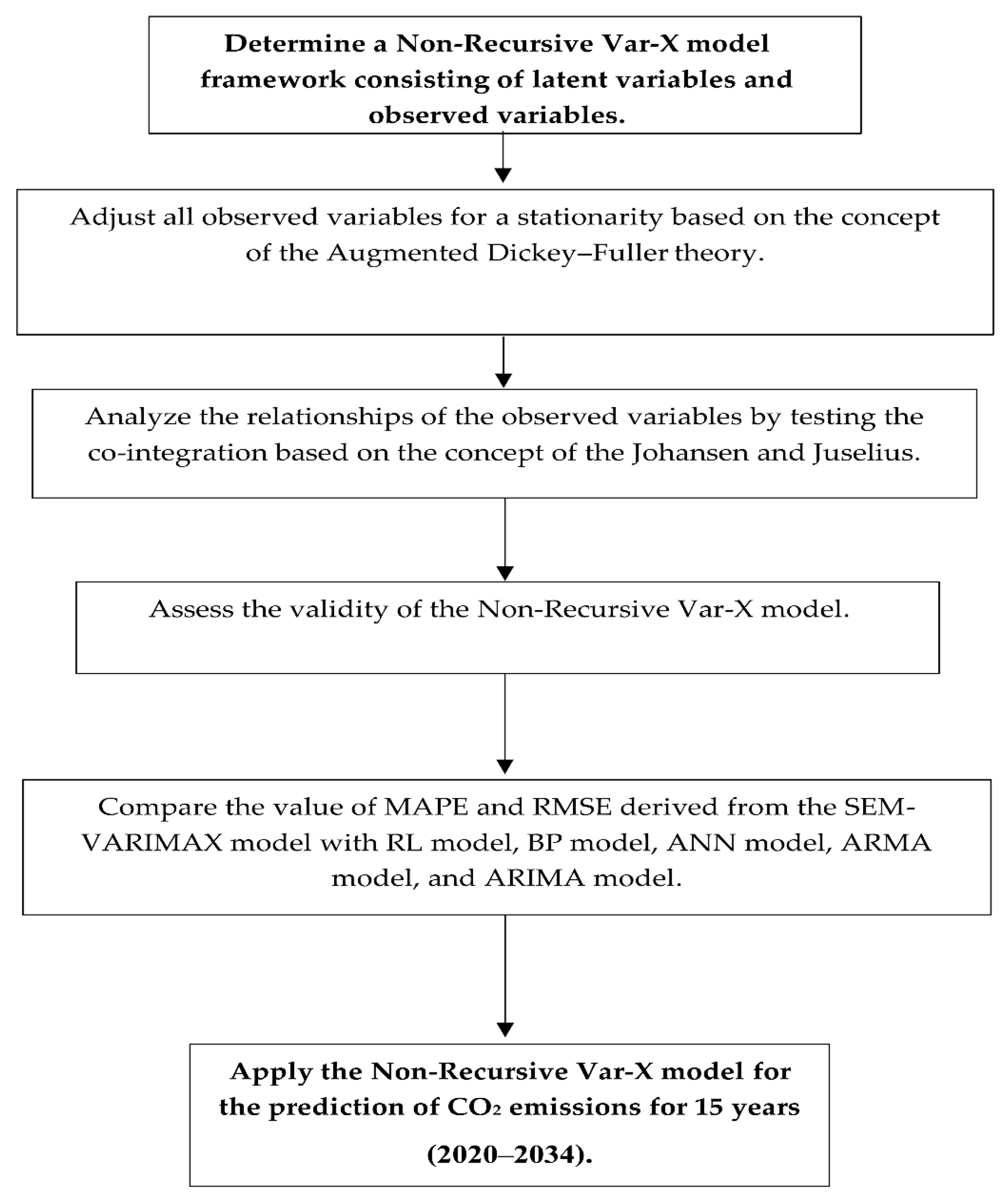
• Ensure all observed variables to be stationary at the first difference level, based on the concept of the augmented Dickey–Fuller [51].
• Analyze the co-integration, based on the concept of the Johansen and Juselius [52,53,54].
• Test the validity of the second order autoregressive-SEM [55,56,57].
• Compare the performance of the second order autoregressive-SEM with other models, including ML model, BP model, ANN model, gray model, and ARIMA model. through the performance measures of MAPE and RMSE [57,58].
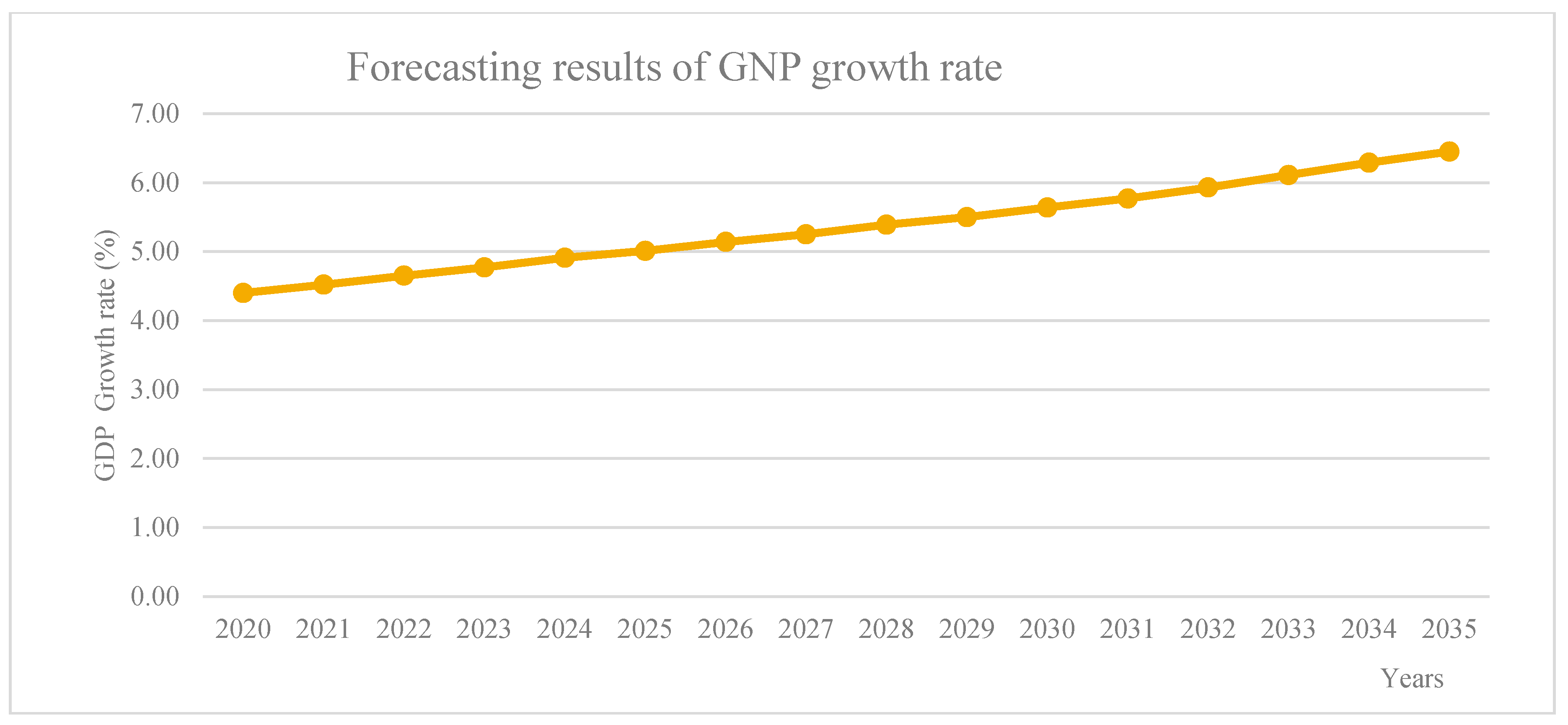
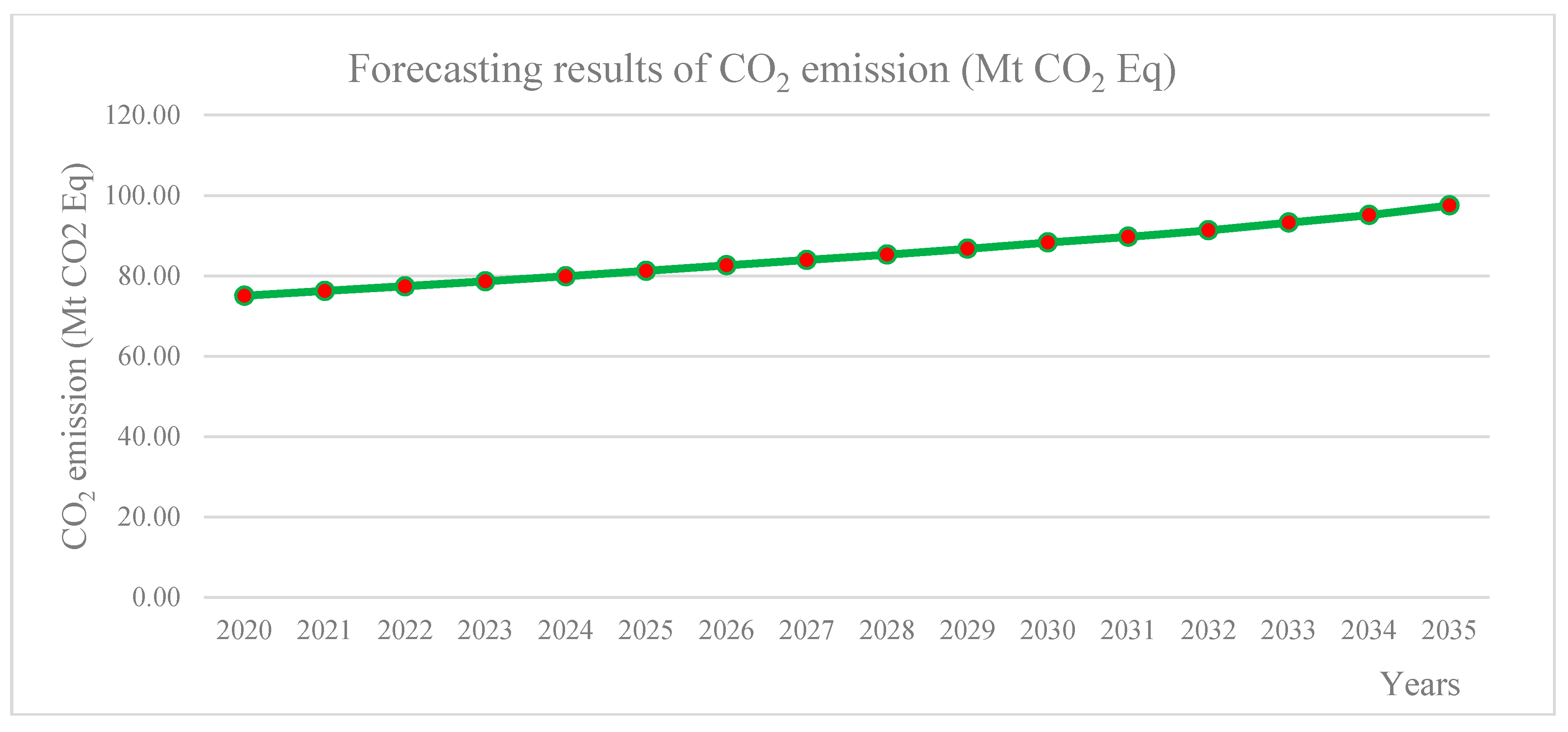
• Forecast GNP and CO₂ emission by deploying the second order autoregressive-SEM for the years 2020 to 2035, as shown in the following diagram.

3. Materials and Methods

3.1. Stationary

Time series of variable $X_t$ will be constant when there are attributes as follows [57,59,60]:

(1) Mean of variable $X$ of each time series t will be constant value or can be written as $\mathrm{E}\left(X_t\right)=\mu ,t=1,2,\dots ,T$

(2) Variance of variable $X$ of each time series t will be a constant value or can be written as $\mathrm{var}\left(X_t\right)=\mathrm{E}{\left(X_t-\mu \right)}^2={\sigma }_x^2,t=1,2,\dots ,T$

(3) Variance of variable $X$ at $t_1$ and $t_2\left(t_1\ne t_2\right)$ will be a constant value or can be written as ${\gamma }_t=\mathrm{cov}\left(X_{t_1},X_{t_2}\right)$ where $t_1-t_2=\tau$ which means the joint variance between time series $\left(X_t\right)$ at different time intervals will depend on distance of both time series $\tau$ (or joint variance between time series $\left(X_t\right)$ at different time intervals will not depend on variable $X_t$ at $t_1$ or $t_2$). Therefore, we can describe as ${\gamma }_{\tau }=\mathrm{cov}\left(X_{t_1},X_{t_2}\right)=\mathrm{cov}\left(X_{t_1+k},X_{t_2+k}\right)$ where k is a constant value. With this attribute, there will be an additional attribute, which is that the variance of variable $X$ at $t$ can be written as $\mathrm{var}\left(X_t\right)=\mathrm{cov}\left(X_{t_1},X_{t_2}\right)={\gamma }_0$ and joint variance of time series $X$ at $t_1$ and $t_2$ are equal to joint variance of time series $X$ at $t_2$ and $t_1$ and can be written as $\mathrm{cov}\left(X_{t_1},X_{t_2}\right)=\mathrm{cov}\left(X_{t_2},X_{t_1}\right)$ or ${\gamma }_{\tau }={\gamma }_{-\tau }$.

When time series $X_t$ is constant $\left(t=1,2,\dots ,T\right)$ it is found that the related parameter will be $T+1$ which is $\mu ,{\sigma }_x^2,{\gamma }_{\tau }{\left(\tau =t_2-t_1,t_1\ne t_2\right)}^2$. In considering parameter ${\gamma }_t$ it is found that the increasing information of $T$ will increase parameter value of ${\gamma }_t$ too. In case of time series $X_t$ at 2 time interval have correlation (or ${\gamma }_t\ne 0$) time series $X_t$ is memory of the process [60].

In considering parameter value $\mu$, which represents the mean of the time series $X_t$ and parameter value ${\sigma }_x^2$ on the variance of time series $X_t$, both will be constant values throughout the distance.

3.1.1. Sequence $p$: Autoregressive Model

Sequence p: Autoregressive Model can be written in equation as AR$\left(p\right)$ as follows [61]:

$$X_t=a_0+a_1{X}_{t-1}+a_2{X}_{t-2}+\dots +a_p{X}_{t-p}+{\epsilon }_t$$

(1)

where $X_t$ is the time series, $a_0,\dots ,a_p$ is the parameters, and ${\epsilon }_t$ is the error term. Equation (1) can also be written as

$$a\left(L\right)X_t=a_0+{\epsilon }_t$$

(2)

where $L$ is the lag operator, $a\left(L\right)=1-a_{1}L-a_2{L}^2-\dots -a_p{L}^p$ mean of time series $X_t$ in the form of AR$\left(p\right)$ as follows:

$$\mu =\frac{{\mu }_0}{1-\left(a_1+a_2+\cdots +a_p\right)}$$

(3)

where $\mu$ is the mean, and variance of TAC and TPAC of time series $X_t$ in the form of AR$\left(p\right)$ can be found by using the concept of the previous case, including the condition which causes $X_t$ in the form of AR$\left(p\right)$ to be constant, the same as before, which is the “absolute value of equation $1-a_{1}L-a_2{L}^2-\dots -a_p{L}^p=0$ must be more than 1” despite the greater complexity. However, TAC and TPAC values can be summarized as follows:

The TAC value of time series $X_t$, according to the AR$\left(p\right)$ model, may be decreased gradually as exponential or waving as exponential. TPAC value of time series $X_t$, as per model AR$\left(p\right)$ at lag 1 to $\left(p\right)$, will not be 0 and will be 0 from $p+1$ onward, or it can be said that TPAC cuts off after lag $\left(p\right)$.

3.1.2. Stationary Test of Time Series

As described in the previous topic, if $X_t\sim I\left(d\right)$, ${\Delta }^d{X}_t$ will be a constant time series (at $d\ge 1$). In practical application, two statisticians—Dickey and Fuller—proposed a statistical method to test the constant of a time series, which can be used to test by what rank variance $\left(d\right)$ can be made to be the constant of a time series. The details of testing can be described as follows [62]:

Consider time series AR(1) as follows:

$$X_t=\rho X_{t-1}+{\epsilon }_t\text{ where }{X}_0=0$$

(4)

$$\mathrm{at}t=1X_1=\rho X_0+{\epsilon }_1={\epsilon }_1$$

$$\mathrm{at}t=2X_2=\rho X_1+{\epsilon }_2={\epsilon }_2+\rho {\epsilon }_1$$

$$\mathrm{at}t=3X_3=\rho X_2+{\epsilon }_3={\epsilon }_3+\rho {\epsilon }_2+{\rho }^2{\epsilon }_1$$

We can draw the equation, in general, as follows:

$$X_t={\epsilon }_t+{\rho }^1{\epsilon }_{t-1}+{\rho }^2{\epsilon }_{t-2}+\dots +{\rho }^{t-1}{\epsilon }_1$$

$$\mathrm{Or}{X}_t={\displaystyle \sum _{i=0}^{t-1}{\rho }^i{\epsilon }_{t-i}}$$

(5)

When $\rho =1$, Equation (5) will describe time series $X_t$ in the form of a random walk equation. In practice, it is usually found that time series in economics, business and finance will be in this format. Also if $0<\rho <1$, Equation (5) will describe an unpredictable event in the past; the further in the past, the lesser the impact to $X_t$ at the present time. The time series of economics, business, and finance are the same.

If $p>1$, Equation (5) will describe the unpredictable event in the past; the further in the past, the greater the impact to $X_t$ at the present time. In reality, there is no variable in economics, business or finance that has this character described by $-1<\rho <0$. Equation (5) describes the value of variable $X_t$, which is accumulated from positive and negative unpredictable events that will have decreasing impact on $X_t$ as time goes by.

Theoretically, if $\rho <-1$, it will be also be move up and down (representing positive and negative events), but it will have increasing impact on $X_t$ as time goes by. In reality, variables in economics, business and finance do not exist in this format.

In summary, a time series in the form of AR(1) will not be constant when $\left|\rho \right|\ge 1$ and will be constant when $\left|\rho \right|<1$. In practice, only two cases will be used, which are $\rho =1$ or $0<\rho <1$.

Therefore, both statisticians, Dickey and Fuller, [51,63] proposed time series testing on the basis that either the time series has a random walk trend, or it does not, with the hypothesis as follows:

$$\begin{gathered} H_0:\rho =1\left(\mathrm{means}\mathrm{time}\mathrm{series}\mathrm{has}\mathrm{a}\mathrm{random}\mathrm{walk}\mathrm{trend}\right) \\ {H}_1:\left|\rho \right|<1\left(\mathrm{means}\mathrm{time}\mathrm{series}\mathrm{has}\mathrm{no}\mathrm{random}\mathrm{walk}\mathrm{trend}\right) \end{gathered}$$

Due to the rejection of the primary hypothesis, $\rho$’s value in the hypothesis will be between 0 and 1 $\left(0<\rho <1\right)$; therefore, a secondary hypothesis can be briefly written as $H_1:\left|\rho \right|<1$. The above hypothesis can be done using $t^{*}$ as per the formula that follows:

$$t^{*}=\frac{\widehat{\rho }-1}{se\left(\widehat{\rho }\right)}$$

Replacing $\rho$ under the primary hypothesis (which is $\rho =1$) will make equation AR(1) to be as follows:

$$X_t=X_{t-1}+{\epsilon }_t\text{ or }\alpha \left(L\right)X_t={\epsilon }_t$$

where $\alpha \left(L\right)=1-L$ which will make the root of equation $\alpha \left(L\right)=0$, which is 1. This is called “unit root” testing.

However, both statisticians Dickey and Fuller found that if the parameter value under the primary hypothesis $p=1$ is true, then estimation by the least square method $\left(\widehat{\rho }\right)$ will not result in a normal distribution even if the sample size is large. That is, the hypothesis testing cannot use the crisis value from a normal distribution table, t distribution table, or F distribution table. Therefore, both statisticians calculated a new crisis value by dividing the crisis value to be used in unit root testing as follows:

$$X_t=\rho X_{t-1}+{\epsilon }_t$$

(6)

$$X_t={\beta }_0+\rho X_{t-1}+{\epsilon }_t$$

(7)

$$X_t={\beta }_0+{\beta }_{1}t+\rho X_{t-1}+{\epsilon }_t$$

(8)

From Equation (8), there is a specified trend variable and a constant value join in the Unit Root testing, but only constant value in Equation (7). Equation (6) has no constant value, and a trend to be determined. To choose among Equations (6)–(8), there are principles, as follows:

When we draw a graph of a time series to test a constant, if it is found that time series moves up and down around 0, then Equation (6) should be selected; if the series has no increasing or decreasing trend over time, but moves up and down around one constant value, then Equation (7) should be selected; finally, if the time series has a trend that moves up or down as time passes, then Equation (8) should be selected.

Taken $X_{t-1}$ to subtract from both side of Equations (6)–(8), will result as follows:

$$\Delta X_t=\gamma X_{t-1}+{\epsilon }_t$$

(9)

$$\Delta X_t={\beta }_0+\gamma X_{t-1}+{\epsilon }_t$$

(10)

$$\Delta X_t={\beta }_0+{\beta }_{1}t+\gamma X_{t-1}+{\epsilon }_t$$

(11)

where $\gamma =\rho -1$, we can use equation in testing whether there is a constant or not in time series $X_t$ by setting the primary hypothesis and secondary hypothesis as follows:

$$\begin{gathered} H_0:\gamma =0(\mathrm{equal}\mathrm{to}{H}_0:\rho =1) \\ {H}_1:\gamma <0(\mathrm{equal}\mathrm{to}{H}_0:\rho <1) \end{gathered}$$

To utilize Equations (9)–(11) in unit root testing, the calculation of $t$ will be easier as follows:

$$t^{*}=\frac{\widehat{\gamma }}{se\left(\widehat{\gamma }\right)}$$

Calculating the statistical value of $t^{*}$ will require the same formula used for testing to find out the parameter value in a regression equation different from 0, with significance or not, acquainted to $t^{*}$ value. Here, usually Equations (9)–(11) are used in Unit Root testing.

3.2. Second Order Autoregressive—SEM

The second order autoregressive structure equation model or second order autoregressive-SEM, is a model from which stationary variables have been taken in order to analyze a model with details as follows:

The model equation structure entails a linkage of latent variables which are abstract and cannot be measured directly, but can be done via a visible item, manifest, item measurement or indicator. To know the right correlation of indicators and latent variables, the relationship of latent variables should be studied in advance. The form of specifications can be identified as follows [61]:

(1) Reflective measurement model

Reflective measurement models have long been used to test theory. The principle of this theory states that each indicator is a reflection of a latent variable. The correlation is in the form of how the latent variable impacts the indicator—that is, the latent variable ${\eta }_i$ reflects the indicator $X_{ij}$ which show the reflection by straight line equation as

$$X_{ij}={\lambda }_{ij}{\eta }_i+{\delta }_{ij};j=1,2,\dots ,m$$

(12)

where $X_{ij}$ is the reflective indicator of ${\eta }_i$ weight ${\lambda }_j$ is the influence level at ${\eta }_i$ effect to $X_j$ and ${\delta }_j$ is the discrepancy. There shouldbe no problem with serial correlation, which is $\mathrm{E}\left({\delta }_i{\delta }_j\right)=0;i\ne j$ should be create no measurement error, which is $\mathrm{E}\left({\eta }_i{\delta }_{ij}\right)=0$. And ${\lambda }_{ij}$ should always be positive.

(2) Formative model

The argument against the use of a reflective measurement model is that it is not certain that an indicator correlates positively to a latent variable, and it is not certain that such indicator is the reflection of the given latent variable. The latent variable may incur from indicator and the meaning of latent variable is came from the summary of name and conceptualize of indicator. In this case it is formative model, and the measurement equation is

$${\eta }_i={\gamma }_{i1}{X}_{i1}+{\gamma }_{i2}{X}_{i2}+{\gamma }_{i3}{X}_{i3}+{\varsigma }_i;j=1,2,\dots ,m_i;i=1,2,\dots ,k$$

(13)

where ${\gamma }_{ij}$, which is the influence on $X_{ij}$, effects ${\eta }_i$, and ${\varsigma }_i$ is a disturbance term whereby $\mathrm{E}\left(X_{ij}{\varsigma }_i\right)=0$ there is no error in the variable. In addition, this should agree with the regression equation, in which there is no problem of multicollinearity, no problem of heteroscedasticity, no problem on autocorrelation, and no problem of non-normality.

The formative model differs from the reflective model as follows [4,62]:

(1)

Indicators come from different sources—that is, from specific points of different domains that are non-interchangeable—and, if some indicators are partially cut in the same way as the prior case of reflective indicator, the nature of the construct will vary and the meaning will not conform exactly to theory; there may also be a lack of construct validity.

(2)

Indicators may not be correlated, or some correlation may be positive or negative.

(3)

Indicators will not have error term which is in equation ${\eta }_i={\gamma }_{i1}{X}_{i1}+{\gamma }_{i2}{X}_{i2}+{\gamma }_{i3}{X}_{i3}+{\varsigma }_i$, ${\varsigma }_i$ will be the error of ${\eta }_i$ and not $X_{ij};j=1,2,\dots ,m_i;i=1,2,\dots ,k$, which means the formative measurement model has no measurement error.

(4)

Each value of equation of formative measurement model will not be estimated in the form of a simple straight-line regression equation since it will be under-identified. It should be estimated by multiple regression equation only.

High rank model

From the equation ${\eta }_i={\gamma }_{i1}{X}_{i1}+{\gamma }_{i2}{X}_{i2}+{\gamma }_{i3}{X}_{i3}+{\varsigma }_i;j=1,2,\dots ,m_i;i=1,2,\dots ,k$, the correlation of the equation, as per the figure below, will be called a first order measurement model. But it is often found that literature indicates that a construct composed of a multi-dimensional entity that is to replace ${\eta }_i$ can be measured by an indicator as per the figure below. It happens that ${\eta }_i$ is measurable by looking at any of a group of related indicators, called an ‘attribute’ or ‘dimension’—${\eta }_i$, in this case, is a multi-dimensional construct [7,63].

From Figure 2, all constructs combined as i correlated between indicator and dimension, and between dimension and latent variable, need to be correctly identified and associated with equation in any form as follows:

(1) Formative first order and formative second order analysis, as detailed in Figure 1, can be called an ‘aggregated model’, ‘composite model’, ‘emergent model’ or ‘indirect formative model’.

The correlation illustrated in Figure 3 is correlation at dimensions, which are ${\eta }_1,{\eta }_1,\dots ,{\eta }_k$ effects to the construct, which is ${\eta }_w$. The diagram illustrates that the construct is made up of multiple dimensions, which, in turn, are composed of (or defined by) indicators $X_{ij}$. The equation for measurement is:

$${\eta }_i={\gamma }_{i1}{X}_{i1}+{\gamma }_{i2}{X}_{i2}+\dots +{\gamma }_{imi}{X}_{imi}+{\varsigma }_i;j=1,2,\dots ,m_i;i=1,2,\dots ,k$$

(14)

and the structure equation is

$${\eta }_w={\beta }_{w1}{\eta }_1+{\beta }_{w2}{\eta }_2+\dots +{\beta }_{wk}{\eta }_k+\varsigma$$

(15)

(2) Reflective first order and formative second order—the linkage among indicators, dimensions and latent variables, as described in Figure 4.

From Figure 4, it is noticeable that there is error in indicator levels and second order constructs. An easy way to think about this is that dependent variables will always be inexactly measured due to measurement errors and other unidentified factors inherent in the use of reflected effects. In the figure, it is shown that $X_{ij};j=1,2,\dots ,m_i;i=1,2,\dots ,k$ are dependent variables and ${\eta }_w$ is also a dependent variable, so there are almost certainly errors in both. The measurement equation model (Level 1) is as follows:

$$\begin{array}{l}{X}_{1j}={\lambda }_{1j}{\eta }_1+{\delta }_{1j};j=1,2,\dots ,m_1\\ X_{2j}={\lambda }_{2j}{\eta }_2+{\delta }_{2j};j=1,2,\dots ,m_2\\ ⋮\end{array}$$

$$X_{kj}={\lambda }_{kj}{\eta }_k+{\delta }_{kj};j=1,2,\dots ,m_k$$

(16)

Level 2 variable is:

$${\eta }_w={\beta }_{w1}{\eta }_1+{\beta }_{w2}{\eta }_2+\dots +{\beta }_{wk}{\eta }_k+\varsigma$$

(17)

(3) Formative first order, reflective second order—the model is as shown in Figure 5:

In Figure 5, the measurement model is a formative model and the second order construct is a reflective model. Variance is found only with the dimension variables cause of each variance is unclear and may be caused by unidentified indicators, or by some other latent variable over ${\eta }_1,{\eta }_2,\dots ,{\eta }_k$ (that is, the variances are met at the dimension variables) so this type of model is not found in literature. The reasons are that (1) it is difficult to analyze dimension variables due to the inability to identify the effect on each factor and its source, and (2) formative indicators cannot replace each other. Therefore, reflective second order AR-SEM is a model which is different from traditional models used in the past and is appropriate for use in both short term and long term predictions.

3.3. Measurement of the Forecasting Performance

In this research, we tested the performance of the second order autoregressive-SEM by using MAPE and RMSE and comparing the results with those of existing models such as the ML model, BP model, ANN model, gray model, and ARIMA model. The calculation equations are shown as follows [57,58,59,63]:

$$MAPE=\frac{1}{n}{\displaystyle \sum _{i=1}^n\left|\frac{{\widehat{y}}_i-y_i}{y_i}\right|}$$

(18)

$$RMSE=\sqrt{\frac{1}{n}{\displaystyle \sum _{i=1}^n{\left({\widehat{y}}_i-y_i\right)}^2}}$$

(19)

4. Empirical Analysis

4.1. Screening Influencing Factors for Model Input

In this paper, the second order autoregressive-SEM is used to analyze the impact and relationship of the causal factors, and forecast GNP and CO₂ emission for of the upcoming 16 years (2020–2035). The latent variables comprise political policy $(Politi)$, the economy $(Econ)$, and the environment $(Environ)$, where the observed variables are national income $(NI)$, urbanization rate $(Ur)$, industrial structure $(Si)$, net exports $(E-I)$, foreign investment $(FI)$, foreign tourism $(Ft)$, employment $(Em)$, government investment $(Gi)$, government subsidy $(Gs)$, technology investment $(Te)$, energy consumption $(Ec)$, energy intensity $(EI)$, and carbon dioxide emission $(C{O}_2)$. Therefore, in order to construct the second order autoregressive-SEM, we must begin with all the causal factors, with their characteristic stationarity, at the first different level by comparing the outcomes of the forecast with MacKinnon Critical Value at the level (1) based on this Augmented Dickey–Fuller theory. In this paper, at the level (0), all causal factor variables are non-stationary, and they cannot be used to construct the model. In addition, we have taken a logarithm, so that all variables become linear, as illustrated in

Table 1. Stationary test at first difference I (1).

Stationary at First Difference I (1)		MacKinnon Critical Value
Variables	Tau test	1%	5%
$\Delta \ln (NI)$	−5.75 ***	−4.05	−3.25
$\Delta \ln \left(\mathrm{Ur}\right)$	−5.02 ***	−4.05	−3.25
$\Delta \ln \left(\mathrm{Si}\right)$	−5.11 ***	−4.05	−3.25
$\Delta \ln (\mathrm{E}-\mathrm{I})$	−4.99 ***	−4.05	−3.25
$\Delta \ln \left(\mathrm{FI}\right)$	−4.35 ***	−4.05	−3.25
$\Delta \ln \left(\mathrm{Ft}\right)$	−4.71 ***	−4.05	−3.25
$\Delta \ln \left(\mathrm{Em}\right)$	−4.69 ***	−4.05	−3.25
$\Delta \ln \left(\mathrm{Gi}\right)$	−4.25 ***	−4.05	−3.25
$\Delta \ln \left(\mathrm{Gs}\right)$	−4.31 ***	−4.05	−3.25
$\Delta \ln \left(\mathrm{Te}\right)$	−5.55 ***	−4.05	−3.25
$\Delta \ln \left(\mathrm{Ec}\right)$	−5.45 ***	−4.05	−3.25
$\Delta \ln \left(\mathrm{Ei}\right)$	−4.65 ***	−4.05	−3.25
$\Delta \ln ({\mathrm{CO}}_2)$	−5.81 ***	−4.05	−3.25

Note: $NI$ is the nation income, $Ur$ is the urbanization rate, $Si$ is the industrial structure, $E-I$ is the is the net exports, $FI$ is the indirect foreign investment, $Ft$ is the foreign tourism, $Em$ is the employment, $Gi$ is the government investment, $Gs$ is the government subsidy, $Te$ is the technology investment, $Ec$ is the energy consumption, $EI$ is the energy intensity, $C{O}_2$ is the carbon dioxide emission, *** denotes a significance, $\mathsf{\alpha }$ = 0.01, compared to the Tau test with the MacKinnon critical value, $\mathsf{\Delta }$ is the first difference, and $\ln$ is the natural logarithm.

.

Table 1 shows that all variables analyzed here are stationary at the first difference level. The Tau test has a value greater than the MacKinnon critical value at all significance level of 1% and 5%. They become stationary at the same level (1) for all values. Thus, we can apply all variables to analyze co-integration by using the concept of Johansen and Juselius, as shown in

Table 2. Co-integration test by Johansen and Juselius.

Variables	Co-Integration Value		MacKinnon Critical Value
$\Delta \ln \left(\mathrm{NI}\right)$, $\Delta \ln \left(\mathrm{Ur}\right)$, $\Delta \ln \left(\mathrm{Si}\right)$, $\Delta \ln (\mathrm{E}-\mathrm{I})$, $\Delta \ln \left(\mathrm{FI}\right)$, $\Delta \ln \left(\mathrm{Ft}\right)$, $\Delta \ln \left(\mathrm{Em}\right)$, $\Delta \ln \left(\mathrm{Gi}\right)$, $\Delta \ln \left(\mathrm{Gs}\right)$, $\Delta \ln \left(\mathrm{Te}\right)$,$\Delta \ln \left(\mathrm{Ec}\right)$, $\Delta \ln \left(\mathrm{Ei}\right)$, $\Delta \ln ({\mathrm{CO}}_2)$	Trace statistic test	Max-Eigen statistic test	1%	5%
	205.05 ***	102.11 ***	15.25	10.05

*** denotes significance α = 0.01.

.

4.2. Analysis of Co-Integration

As shown in Table 2, the co-integration test by Johansen and Juselius found that the stationary variables at the first difference, all with co-integration at the same level along with the Trace statistic test was 205.05, and the maximum Eigen statistic test was 102.11. Those two values are greater than MacKinnon critical values at the significance level of 1% and 5%. Hence, we can use all stationary variables at the first difference with co-integration at the same level to analyze the impact of the relationship of the causal factors in the second order autoregressive-SEM, as shown in Figure 6 and

Table 3. Results of relationship size analysis of the Second Order Autoregressive-SEM.

Dependent Variables	Type of Effect	Independent Variables
		$\mathbf{Political}\mathbf{Policy}(\mathit{P}\mathit{o}\mathit{l}\mathit{i}\mathit{t}\mathit{i})$	$\mathbf{Economy}(\mathit{E}\mathit{c}\mathit{o}\mathit{n})$	$\mathbf{Environment}(\mathit{E}\mathit{n}\mathit{v}\mathit{i}\mathit{r}\mathit{o}\mathit{n})$	$\mathbf{Error}\mathbf{Correction}\mathbf{Mechanism}(\mathit{E}\mathit{C}{\mathit{T}}_{\mathit{t}-1})$
Political policy $(Politi)$	DE	-	0.35 ***	0.15 **	−0.31 ***
	IE	-	0.12 ***	0.04 **	-
Economy $(Econ)$	DE	0.71 ***	-	0.25 **	−0.59 ***
	IE	0.15 ***	-	0.01 **	-
Environment $(Environ)$	DE	0.59 ***	0.69 ***	-	−0.05 ***
	IE	0.02 ***	0.35 ***	-	-

Note: In the above, *** denotes significance $\mathsf{\alpha }$ = 0.01, ** denotes significance α = 0.05, ${\chi }^2/df$ is 1.20, $\mathrm{RMSEA}$ is 0.05, $\mathrm{RMR}$ is 0.001, $\mathrm{GFI}$ is 0.92, $\mathrm{AGFI}$ is 0.92, R-squared is 0.95, the F-statistic is 255.05 (probability is 0.00), the ARCH test is 20.01 (probability is 0.1), the LM test is 1.15 (probability is 0.10), DE is the direct effect, and IE is the indirect effect.

.

4.3. Formation of Analysis Modeling with the Second Order Autoregressive-SEM

The second order autoregressive-SEM is a model indicating the relationship of the causal factors, and it is stationary and co-integrated at the same level. The results of the analysis are illustrated below.

Figure 6 demonstrates the impact of the causal factors in the Second Order Autoregressive-SEM. The latent variables are political policy $(Politi)$, the economy $(Econ)$, and the environment $(Environ)$, where the observed variables are national income $(NI)$, urbanization rate $(Ur)$, industrial structure $(Si)$, net exports $(E-I)$, foreign investment $(FI)$, foreign tourism $(Ft)$, employment $(Em)$, government investment $(Gi)$, government subsidy $(Gs)$, technology investment $(Te)$, energy consumption $(Ec)$, energy intensity $(EI)$, and carbon dioxide emission $(C{O}_2)$. In addition, the second order autoregressive-SEM can reflect on the adjustment ability toward equilibrium of the latent variables with different magnitudes. This criterion can be seen in the error correction mechanism $(\mathrm{EC}{\mathrm{T}}_{\mathrm{t}-1})$, as part of the results shown in Table 3.

Table 3 illustrates the parameters of the second order autoregressive-SEM at the statistical significance levels of 1% and 5%. When validating the second order autoregressive-SEM, the goodness of fit value passes all criteria—RMSEA and RMR are not far from 0, while GFI and AGFI values approach 1. Furthermore, testing the best model of the second order autoregressive-SEM shows that heteroskedasticity, multicollinearity, autocorrelation, and non-normality are absent. Therefore, the second order autoregressive-SEM presents causal relationships of the latent variables, including political policy $(Politi)$, economy $(Econ)$, and environment $(Environ)$. The analysis results show that political policy $(Politi)$ has a direct effect on the economy $(Econ)$ at about 71% with a significance level of 1%; political policy $(Politi)$ has a direct effect on the environment $(Environ)$ at about 59% with a significance level of 1%; economy $(Econ)$ has a direct effect on political policy $(Politi)$ at about 35% with a significance level of 1%; economy $(Econ)$ has a direct effect on environment $(Environ)$ at about 69% with a significance level of 1%; environment $(Environ)$ has a direct effect on political policy $(Politi)$ at about 15% with a significance level of 5%, and Environment $(Environ)$ has a direct effect on economy $(Econ)$ at about 25% with a significance level of 5%.

However, the study has evidenced that the economy $(Econ)$ has an adjustment ability to equilibrium, where the error correction mechanism $(EC{T}_{t-1})$ is about 59%, greater than any other variable. The next variable is political policy $(Politi)$, whose error correction mechanism $(EC{T}_{t-1})$ is about 31%, while environment $(Environ)$ has the weakest adjustment ability, with an error correction mechanism $(EC{T}_{t-1})$ measured at about 5%.

Therefore, we tested the performance of the second order autoregressive-SEM using MAPE and RMSE and compared those two values with those of the other models—the ML model, BP model, ANN model, gray model, and ARIMA model—as shown in

Table 4. The performance monitoring of the forecasting models.

Forecasting Model	MAPE (%)	RMSE (%)
ML model	22.25	20.59
BP model	15.22	15.65
ANN model	12.05	13.11
gray model	9.25	10.59
ARIMA model	4.94	6.88
Second Order Autoregressive-SEM	1.02	1.51

.

Table 4 presents the second order autoregressive-SEM measured by MAPE and RMSE along with a comparison of such values with other past models. Such values are estimated to be 1.02% and 1.51% for MAPE and RMSE, respectively. These results show that the second order autoregressive-SEM is the most suitable model for long-term forecasting (2020–2035). The performance of the ARIMA model, gray model, ANN model, BP model, and ML model ranked below that of the second order autoregressive-SEM, ranked from second to sixth, respectively. Therefore, the second order autoregressive-SEM has been identified through this process as the most appropriate forecasting model, allowing us to predict GNP and CO₂ emission in the long term, as shown in the table.

4.4. A Forecasting Model on the Changes of GNP and CO₂ Emission Based on the Second Order Autoregressive-SEM

In the forecasting presented here, second order autoregressive-SEM was used to predict changes in GNP and CO₂ emission in Thailand for the next 16 years (2020–2035) based on government policy, as illustrated in Figure 7 and Figure 8.

Figure 7 shows that the GNP from 2020–2035, under the Industry 4.0 policy, is projected to steadily increase from 2020 to 2035, with a 6.45% rate of change. This predicted growth rate predicts a significant positive impact on the economy of Thailand resulting from the government policy.

Figure 8 shows that the CO₂ emission from 2020 to 2035, under the same policy and government power, is predicted to increase to an estimated 97.52 Mt CO₂ Eq. by 2035. This CO₂ emission is greater than the limit of environment hazards and disaster prevention ratio set by the government, where the policy states not to exceed 80 Mt CO₂ Eq. in the ending period of 2035.

5. Conclusions and Discussion

This research proposes the adoption of second order autoregressive-SEM by using advanced statistics to analyze the influential magnitude of causal relationships, and to forecast such influence on economic and environmental factors under the Industry 4.0 policy imposed by the federal government of Thailand. The software utilized in the analysis was LISREL, which is the most suitable software for this type of advanced statistics. This research was carried out through application of research principles considering the characteristics of the causal factors in establishing a long-term forecasting model. In choosing all causal factors for this model, only identified actual causal factors were taken for analysis by ensuring each factor become stationary at the first difference, while all variables were co-integrated at the same level. The variables are national income ($\Delta \ln \left(\mathrm{NI}\right)$), urbanization rate ($\Delta \ln \left(\mathrm{Ur}\right)$), industrial structure ($\Delta \ln \left(\mathrm{Si}\right)$), net exports ($\Delta \ln (\mathrm{E}-\mathrm{I})$), foreign investment ($\Delta \ln \left(\mathrm{FI}\right)$), foreign tourism ($\Delta \ln \left(\mathrm{Ft}\right)$), employment ($\Delta \ln \left(\mathrm{Em}\right)$), government investment ($\Delta \ln \left(\mathrm{Gi}\right)$), government subsidy ($\Delta \ln \left(\mathrm{Gs}\right)$), technology investment ($\Delta \ln \left(\mathrm{Te}\right)$), energy consumption ($\Delta \ln \left(\mathrm{Ec}\right)$), energy intensity ($\Delta \ln \left(\mathrm{Ei}\right)$), and carbon dioxide emission ($\Delta \ln (\mathrm{C}{\mathrm{O}}_2)$). Such variables were selected in order to develop the second order autoregressive-SEM. This model has validity and features of the best model, heteroskedasticity, multicollinearity, autocorrelation and non-normality are absent. Hence, it can reflect actual relationships of latent variables, including political policy $(Politi)$, economy $(Econ)$, and environment $(Environ)$. It also shows us the magnitude of impact for both direct and indirect effects in the model. Furthermore, the three latent variables have direct effect and indirect effect at the significance level of 1% and 5%.

Moreover, the second order autoregressive-SEM, as measured by MAPE and RMSE, outperformed other models, ARIMA model, gray model, ANN model, BP model, and ML model, used by the government as a tool for formulating policies for Thailand in the past. Hence, the second order autoregressive-SEM is found suitable to use for a long-term forecasting (2020–2035), as claimed by Oh and Shin [16] under the title of A Study on the Relationship between Analysts Cash Flow Forecasts Issuance and Accounting Information, Jiang et al. [41] under the title of Comparison of Forecasting India’s Energy Demand Using an MGM, ARIMA Model, MGM-ARIMA Model, and BP Neural Network Model, Wang et al. [42] under the title of Prediction of the Energy Demand Trend in Middle Africa—A Comparison of MGM, MECM, ARIMA and BP Model, Ma et al. [43] under the title of Predicting Coal Consumption in South Africa Based on Linear (Metabolic Grey Model), Nonlinear (Non-Linear Grey Model), and Combined (Metabolic Grey Model-Autoregressive Integrated Moving Average Model) Models, Boyd et al. [44] under the title of Influent Forecasting for Wastewater Treatment Plants in North America, Al-Douri et al. [45] under the title of Time Series Forecasting Using a Two-Level Multi-Objective Genetic Algorithm: A Case Study of Maintenance Cost Data for Tunnel Fans, and Alsharif et al. [46] under the title of Time Series ARIMA Model for Prediction of Daily and Monthly Average Global Solar Radiation: The Case Study of Seoul, South Korea.

The model, when put to use, forecasts significant and steady economic growth as measured by GNP. At the same time, carbon dioxide emission $(C{O}_2)$, as an environmetal indicator, is forecast to increase continuously from 2020–2035, and is further projected to exceed the limit set by Thailand of 80 Mt CO₂ Eq. (2035). By 2035, it is predicted that the carbon dioxide emission $(C{O}_2)$ will climb to 97.52 Mt CO₂ Eq.

This study indicates that the Industry 4.0 policy implemented by the government in Thailand is still inefficient, and that it will not lead to sustainability in the future. The study further shows that the error correction mechanism of the environmental aspect has the weakest ability to adjust toward equilibrium as compared to the economy and political policy, respectively. The previous implementation of past policies has led to economic growth but has also significantly damaged the environment. This phenomenon, if continued, will contribute negatively to the future of Thailand. Moreover, if the environment is devastated, it will be very difficult to retreat and recover. Therefore, the government needs to adopt new tools for formulating the national policies and planning in order to prevent losses that cannot be recovered in the future.

As for recommendations for future applications of this research, the researchers created a high-quality second order autoregressive-SEM to replace the old models used in the past. The second order autoregressive-SEM comes with good validity and distinctive features, making it different from other existing models. This is because the model considers the features of causal factors, and deep understanding of modelling was made as to generate the best model. This helps indicate the impact magnitude of causal factors in both direct and indirect effects while reflecting the adjustment ability to equilibrium. Therefore, if the government is determined to continue implementing and enforcing the Industry 4.0 policy in Thailand, then it must proceed with caution and prudence, while making use of quality tools to determine the outcomes and achieve the optimal positive effect of the national strategy in the long term. Therefore, selecting this tool for national policy formulation and planning becomes significant and necessary in order to successfully implement policies of the highest quality and efficiency. In addition to this importance, with the application of this research outcome in different contexts and sectors, future research should ensure the validity of the model, especially the estimated values from the model, so as to reduce potential errors or spuriousness. Also, they should consider certain variables, that are stationary and co-integrated in the same level for their research. This consideration will allow them to better understand direct and indirect effects.

An additional benefit of the model developed in this research is that it is an instrumental model that shows the impact magnitude. If any change occurs from one side of the model’s equations, it will also affect the projected outcomes on the other side, with different impact magnitude. Hence, the government has to take into account clearly how the plans are to be implemented in order to minimize the negative impact on the environment and set goals in order to create appropriate outcomes. This concern can be addressed by using the Second Order Autoregressive-SEM described in this research as a guide to formulation of the right policies for different sectors of the Thai economy.

This limitation of this research is that some causal factors could not be taken into account because the government does not allow those factors to float freely in the economy. For instance, all oil prices in the country are subject to government intervention from time to time, so they do not reflect the actual prices from a global market. Other variables could include foreign investment projects that are not specified in the national strategy. All these limitations are seen to be important elements in the Industry 4.0 policy, and therefore they cannot be used as variables in this study’s model.

References

1. Office of the National Economic and Social Development Board (NESDB). Available online: http://www.nesdb.go.th/nesdb_en/more_news.php?cid=154&filename=index (accessed on 15 June 2019).
2. National Statistic Office Ministry of Information and Communication Technology. Available online: http://web.nso.go.th/index.htm (accessed on 20 June 2019).
3. Sutthichaimethee, P.; Dockthaisong, B. A Relationship of Causal Factors in the Economic, Social, and Environmental Aspects Affecting the Implementation of Sustainability Policy in Thailand: Enriching the Path Analysis Based on a GMM Model. Resources 2018, 7, 87. [Google Scholar] [CrossRef]
4. Sutthichaimethee, P.; Kubaha, K. The Efficiency of Long-Term Forecasting Model on Final Energy Consumption in Thailand’s Petroleum Industries Sector: Enriching the LT-ARIMAXS Model under a Sustainability Policy. Energies 2018, 11, 2063. [Google Scholar] [CrossRef]
5. Office of Natural Resources and Environmental Policy and Planning. Available online: http://www.onep.go.th (accessed on 15 June 2019).
6. Department of Alternative Energy Development and Efficiency. Available online: http://www.dede.go.th/ewtadmin/ewt/dede_web/ewt_news.php?nid=47140 (accessed on 15 June 2019).
7. Sutthichaimethee, P.; Ariyasajjakorn, D. Forecast of Carbon Dioxide Emissions from Energy Consumption in Industry Sectors in Thailand. Environ. Clim. Technol. 2018, 22, 107–117. [Google Scholar] [CrossRef] [Green Version]
8. Thailand Greenhouse Gas Management Organization (Public Organization). Available online: http://www.tgo.or.th/2015/thai/content.php?s1=7&s2=16&sub3=sub3 (accessed on 16 June 2019).
9. Savaresi, A. The Paris Agreement: An Early Assessment. Environ. Policy Law 2016, 46, 14–18. [Google Scholar]
10. Laina, E. Sustainable Development in Operation. Environ. Policy Law 2016, 46, 47–49. [Google Scholar]
11. Krapp, R. Sustainable Development in the Second Committee. Environ. Policy Law 2016, 46, 10–13. [Google Scholar]
12. Uddin, M.K. Climate Change and Global Environmental Politics: North-South Divide. Environ. Policy Law 2017, 47, 106–114. [Google Scholar] [CrossRef]
13. Moore, P.; Pereira, E.S.; Duggin, G. Developing Environmental Law for All Citizens. Environ. Policy Law 2015, 45, 88–98. [Google Scholar]
14. Savaresi, A. Developments in Environmental Law. Environ. Policy Law 2012, 42, 365–369. [Google Scholar]
15. Mid-term Review. Global Progress in Environmental Law. Environ. Policy Law 2016, 46, 23–27. [Google Scholar]
16. Oh, H.M.; Shin, H.Y. A Study on the Relationship between Analysts Cash Flow Forecasts Issuance and Accounting Information. Evidence from Korea. Sustainability 2019, 11, 3399. [Google Scholar] [CrossRef]
17. He, X.; Yin, C. The Impact of Strategic Deviance on Analysts’ Earnings Forecasts: Evidence from China. Nankai Business Review International. Available online: https://0-www-emerald-com.brum.beds.ac.uk/insight/search?q=Xiqiong+He+Changping+Yin&showAll=true (accessed on 10 June 2019).
18. Dong, G.H.; Zhang, P.; Sun, B.; Zhang, L.; Chen, X.; Ma, N.; Yu, F.; Guo, H.; Huang, H.; Lee, Y.L.; et al. Long-Term Exposure to Ambient Air Pollution and Respiratory Disease Mortality in Shenyang, China: A 12-Year Population-Based Retrospective Cohort Study. Respiration 2012, 84, 360–368. [Google Scholar] [CrossRef] [PubMed]
19. Xu, X.; Ren, W. Application of a Hybrid Model Based on Echo State Network and Improved Particle Swarm Optimization in PM2.5 Concentration Forecasting: A Case Study of Beijing, China. Sustainability 2019, 11, 3096. [Google Scholar] [CrossRef]
20. Xu, X.; Ren, W. Prediction of Air Pollution Concentration Based on mRMR and Echo State Network. Appl. Sci. 2019, 9, 1811. [Google Scholar] [CrossRef]
21. Tsui, W.H.K.; Balli, H.O.; Gilbey, A.; Gow, H. Forecasting of Hong Kong airport’s passenger throughput. Tour. Manag. 2014, 42, 62–76. [Google Scholar] [CrossRef]
22. Mahajan, S.; Chen, L.J.; Tsai, T.C. Short-Term PM2.5 Forecasting Using Exponential Smoothing Method: A Comparative Analysis. Sensors 2018, 18, 3223. [Google Scholar] [CrossRef]
23. Huang, Y.; Yang, L.; Liu, S.; Wang, G. Multi-Step Wind Speed Forecasting Based On Ensemble Empirical Mode Decomposition, Long Short Term Memory Network and Error Correction Strategy. Energies 2019, 12, 1822. [Google Scholar] [CrossRef]
24. Wu, Q.; Lin, H. Short-Term Wind Speed Forecasting Based on Hybrid Variational Mode Decomposition and Least Squares Support Vector Machine Optimized by Bat Algorithm Model. Sustainability 2019, 11, 652. [Google Scholar] [CrossRef]
25. Methaprayoon, K.; Lee, W.-J.; Rasmiddatta, S.; Liao, J.R.; Ross, R.J. Multistage Artificial Neural Network Short-Term Load Forecasting Engine With Front-End Weather Forecast. IEEE Trans. Ind. Appl. 2007, 43, 1410–1416. [Google Scholar] [CrossRef]
26. Fan, S.; Hyndman, R.J. Density Forecasting Electricity Demand in Australian National Electricity Market. In Proceedings of the IEEE Power & Energy Society General Meeting, San Diego, CA, USA, 22–26 July 2012; pp. 1–4. [Google Scholar]
27. Ramos, P.; Oliveira, J.M. A Procedure for Identification of Appropriate State Space and ARIMA Models Based on Time-Series Cross-Validation. Algorithms 2016, 9, 76. [Google Scholar] [CrossRef]
28. Shi, J.; Ding, Z.; Lee, W.J.; Yang, Y.; Liu, Y.; Zhang, M. Hybrid Forecasting Model for Very-Short Term Wind Power Forecasting Based on Grey Relational Analysis and Wind Speed Distribution Features. IEEE Trans. Smart Grid 2014, 5, 521–526. [Google Scholar] [CrossRef]
29. Chen, K.S.; Lin, K.P.; Yan, J.X.; Hsieh, W.L. Renewable Power Output Forecasting Using Least-Squares Support Vector Regression and Google Data. Sustainability 2019, 11, 3009. [Google Scholar] [CrossRef]
30. Lu, P.; Ye, L.; Sun, B.; Zhang, C.; Zhao, Y.; Teng, J. A New Hybrid Prediction Method of Ultra-Short-Term Wind Power Forecasting Based on EEMD-PE and LSSVM Optimized by the GSA. Energies 2018, 11, 697. [Google Scholar] [CrossRef]
31. Guan, W.; Chung, K.; Cheung, K.W.; Sun, X.; Luh, P.B.; Michel, L.D.; Corbo, S. Advanced Load Forecast with Hierarchical Forecasting Capability. In Proceedings of the IEEE Power & Energy Society General Meeting, Vancouver, BC, Canada, 21–25 July 2013. [Google Scholar]
32. Xie, J.; Hong, T.; Stroud, J. Long-Term Retail Energy Forecasting with Consideration of Residential Customer Attrition. IEEE Trans. Smart Grid 2015, 6, 2245–2252. [Google Scholar] [CrossRef]
33. Sun, S.; Wei, L.; Xu, J.; Jin, Z. A New Wind Speed Forecasting Modeling Strategy Using Two-Stage Decomposition, Feature Selection and DAWNN. Energies 2019, 12, 334. [Google Scholar] [CrossRef]
34. Bobinaite, V.; Juozapaviciene, A.; Konstantinaviciute, I. Assessment of Causality Relationship between Renewable Energy Consumption and Economic Growth in Lithuania. Eng. Econ. 2011, 22, 510–518. [Google Scholar] [CrossRef]
35. Soava, G.; Mehedintu, A.; Sterpu, M.; Raduteanu, M. Impact of Renewable Energy Consumption on Economic Growth: Evidence from European Union Countries. Technol. Econ. Dev. Econ. 2018, 24, 914–932. [Google Scholar] [CrossRef]
36. Inglesi-Lotz, R. The impact of renewable energy consumption to economic growth: A panel data application. Energy Econ. 2016, 53, 58–63. [Google Scholar] [CrossRef]
37. Pao, H.T.; Fu, H.C. Renewable energy, non-renewable energy and economic growth in Brazil. Renew. Sustain. Energy Rev. 2013, 25, 381–392. [Google Scholar] [CrossRef]
38. Rafiq, S.; Salim, R. The linkage between energy consumption and income in six emerging economies of Asia an empirical analysis. Int. J. Emerg. Mark. 2011, 6, 50–73. [Google Scholar] [CrossRef]
39. Chontanawat, J.; Hunt, L.C.; Pierse, R. Does energy consumption cause economic growth? Evidence from a systematic study of over 100 countries. J. Policy Model. 2008, 30, 209–220. [Google Scholar] [CrossRef]
40. Sterpu, M.; Soava, G.; Mehedintu, A. Impact of Economic Growth and Energy Consumption on Greenhouse Gas Emissions: Testing Environmental Curves Hypotheses on EU Countries. Sustainability 2018, 10, 3327. [Google Scholar] [CrossRef]
41. Jiang, F.; Yang, X.; Li, S. Comparison of Forecasting India’s Energy Demand Using an MGM, ARIMA Model, MGM-ARIMA Model, and BP Neural Network Model. Sustainability 2018, 10, 2225. [Google Scholar] [CrossRef]
42. Wang, L.; Zhan, L.; Li, R. Prediction of the Energy Demand Trend in Middle Africa—A Comparison of MGM, MECM, ARIMA and BP Models. Sustainability 2019, 11, 2436. [Google Scholar] [CrossRef]
43. Ma, M.; Su, M.; Li, S.; Jiang, F.; Li, R. Predicting Coal Consumption in South Africa Based on Linear (Metabolic Grey Model), Nonlinear (Non-Linear Grey Model), and Combined (Metabolic Grey Model-Autoregressive Integrated Moving Average Model) Models. Sustainability 2018, 10, 2552. [Google Scholar] [CrossRef]
44. Boyd, G.; Na, D.; Li, Z.; Snowling, S.; Zhang, Q.; Zhou, P. Influent Forecasting for Wastewater Treatment Plants in North America. Sustainability 2019, 11, 1764. [Google Scholar] [CrossRef]
45. Al-Douri, Y.K.; Hamodi, H.; Lundberg, J. Time Series Forecasting Using a Two-Level Multi-Objective Genetic Algorithm: A Case Study of Maintenance Cost Data for Tunnel Fans. Algorithms 2018, 11, 123. [Google Scholar] [CrossRef]
46. Alsharif, M.H.; Younes, M.K.; Kim, J. Time Series ARIMA Model for Prediction of Daily and Monthly Average Global Solar Radiation: The Case Study of Seoul, South Korea. Symmetry 2019, 11, 240. [Google Scholar] [CrossRef]
47. Liu, Q.; Shen, Y.; Wu, L.; Li, J.; Zhuang, L.; Wang, S. A hybrid FCW-EMD and KF-BA-SVM based model for short-term load forecasting. CSEE J. Power Energy Syst. 2018, 4, 226–237. [Google Scholar] [CrossRef]
48. Lee, C.W.; Lin, B.Y. Application of Hybrid Quantum Tabu Search with Support Vector Regression (SVR) for Load Forecasting. Energies 2016, 9, 873. [Google Scholar] [CrossRef]
49. Cai, G.; Wang, W.; Lu, J. A Novel Hybrid Short Term Load Forecasting Model Considering the Error of Numerical Weather Prediction. Energies 2016, 9, 994. [Google Scholar] [CrossRef]
50. Liu, B.; Nowotarski, J.; Hong, T.; Weron, R. Probabilistic Load Forecasting via Quantile Regression Averaging on Sister Forecasts. IEEE Trans. Smart Grid 2017, 8, 730–737. [Google Scholar] [CrossRef]
51. Dickey, D.A.; Fuller, W.A. Likelihood ratio statistics for autoregressive time series with a unit root. Econometrica 1981, 49, 1057–1072. [Google Scholar] [CrossRef]
52. Johansen, S.; Juselius, K. Maximum likelihood estimation and inference on cointegration with applications to the demand for money. Oxf. Bull. Econ. Stat. 1990, 52, 169–210. [Google Scholar] [CrossRef]
53. Johansen, S. Likelihood-Based Inference in Cointegrated Vector Autoregressive Models; Oxford University Press (OUP): New York, NY, USA, 1995. [Google Scholar]
54. MacKinnon, J. Critical Values for Cointegration Test in Long-Run Economic Relationships; Engle, R., Granger, C., Eds.; Oxford University Press: Oxford, UK, 1991. [Google Scholar]
55. Sutthichaimethee, P. Forecasting Economic, Social and Environmental Growth in the Sanitary and Service Sector Based on Thailand’s Sustainable Development Policy. J. Ecol. Eng. 2018, 19, 205–210. [Google Scholar] [CrossRef]
56. Sutthichaimethee, P.; Kubaha, K. A Relational Analysis Model of the Causal Factors Influencing CO2 in Thailand’s Industrial Sector under a Sustainability Policy Adapting the VARIMAX-ECM Model. Energies 2018, 11, 1704. [Google Scholar] [CrossRef]
57. Enders, W. Applied Econometrics Time Series; Wiley Series in Probability and Statistics; University of Alabama: Tuscaloosa, AL, USA, 2010. [Google Scholar]
58. Harvey, A.C. Forecasting, Structural Time Series Models and the Kalman Filter; Cambridge University Press: Cambridge, UK, 1989. [Google Scholar]
59. Sutthichaimethee, P.; Ariyasajjakorn, D. The Revised Input-Output Table to Determine Total Energy Content and Total Greenhouse Gas Emission Factors in Thailand. J. Ecol. Eng. 2017, 18, 166–170. [Google Scholar] [CrossRef]
60. Sutthichaimethee, P. Varimax Model to Forecast the Emission of Carbon Dioxide from Energy Consumption in Rubber and Petroleum Industries Sectors in Thailand. J. Ecol. Eng. 2017, 18, 112–117. [Google Scholar] [CrossRef]
61. Sutthichaimethee, P.; Ariyasajjakorn, D. Forecasting Model of Ghg Emission in Manufacturing Sectors of Thailand. J. Ecol. Eng. 2017, 18, 18–24. [Google Scholar] [CrossRef]
62. Sutthichaimethee, P. Modeling Environmental Impact of Machinery Sectors to Promote Sustainable Development of Thailand. J. Ecol. Eng. 2016, 17, 18–25. [Google Scholar] [CrossRef]
63. Sutthichaimethee, P.; Sawangdee, Y. Model of Environmental Problems Priority Arising from the use of Environmental and Natural Resources in Machinery Sectors of Thailand. Environ. Clim. Technol. 2016, 17, 18–29. [Google Scholar] [CrossRef] [Green Version]
Figure 1. The flowchart of the Second Order Autoregressive -SEM.
Joitmc 05 00069 g001
Figure 2. High level of variable correlation.
Joitmc 05 00069 g002
Figure 3. Correlation at dimension.
Joitmc 05 00069 g003
Figure 4. Linkage among indicators, dimensions and latent variables.
Joitmc 05 00069 g004
Figure 5. The variance on dimension variable only.
Joitmc 05 00069 g005
Figure 6. The casual relationship in the Second Order Autoregressive-SEM.
Joitmc 05 00069 g006
Figure 7. The forecasting results for GNP from 2020 to 2035 in Thailand.
Joitmc 05 00069 g007
Figure 8. The forecasting results for CO2 emission from 2020 to 2035 in Thailand.
Joitmc 05 00069 g008