1. Introduction
Open innovation is a business paradigm of innovation process that provides more flexible policy in relation to research, intellectual property, user innovation, aggregate innovation, improving the accuracy of market research and customer focus, synergy between internal and external innovations, viral marketing, innovation implementation and distributed innovation, low research cost [
1,
2,
3,
4,
5,
6,
7,
8,
9].
The boundaries between the firm and its environment have become more permeable. The innovation can easily be transferred in and out between firms and other firms, as well as between firms and creative consumers, which has an impact on the level of the consumer, firm, industry and society [
7,
8].
The search for interrelationships of the main open innovation metrics is one of the important tasks of many branches of economics and political sciences. In view of the obvious and, perhaps, the greatest significance, models and studies on the relationship between gross domestic product (GDP), inflation and unemployment are traditionally of particular interest. Despite the high social significance of the phenomenon under study and many works on this topic, researchers have not yet come to a general conclusion either about the ranking of the significance of the relationship, or about the universality of models for temporal and country differences. Typically, research involves only relationship between two factors [
1,
2,
3].
Countries that are actively introducing open innovation have seen GDP growth continuously for many years. The theoretical basis for the relationship between GDP and innovation began to appear in the works of Solow and Romer [
4,
5]. Growth theories argue that innovation is the main engine of growth: however, the role of open innovation in stimulating economic growth has not been described by growth theories or empirical explanations. Empirical research based on theoretical foundations [
6] examines potential factors for stimulating economic growth. In recent years, economic researchers have been paying more attention to studying the relationship between open innovation and macroeconomic parameters (GDP, inflation, unemployment) of countries [
7,
8,
9].
Thus, the following became classical for many works: the Phillips model (curve) assumes an inverse relationship between inflation and unemployment, and Okun’s model is revealing the relationship between GDP and unemployment; there are many other views, some of which will be considered in the literature review part [
4,
5]. The current state of development of economic science requires the creation of more complex and accurate models, and the development of computer technology is only beneficial to this [
6,
7,
8,
9].
In this paper, we specifically consider the relationship between open innovation and macroeconomic parameters (GDP, inflation, unemployment) in countries around the world. Open innovation is considered as one of the key factors of the economy [
10]. Open innovation affects the economy through many channels, such as economic growth, competitiveness of sectors of the economy, openness of the financial system, quality of life, unemployment rate, openness of international trade, which generates outstripping economic growth. The possibility of bidirectional causal relationships between open innovation and economic growth has also been previously proven [
11]. Thus, the main goal of this work is to study the bi-directional relationship between innovation and macroeconomic parameters. The features of the relationship between innovation and economic growth are the most well researched.
The central assumption is that GDP, inflation and unemployment reflect different aspects of open innovation, and therefore, finding their relationship can become a new predictive open innovation tool or the basis for identifying blocks of countries according to fundamentally new parameters.
First, we specifically evaluate the non-classical approach to identifying groups of countries based on open innovation indicators. The article examines whether open innovation has helped stimulate economic growth. The article also examines whether the expansion of innovation activity was a consequence of rapid economic growth. Second, the paper includes the data from 115 countries were selected to compile the model, which are observations for the algorithm. Each of the countries initially had 90 signs: GDP, inflation and unemployment for 30 years from 1990 to 2019 inclusive, in contrast to existing studies [
5,
6,
7,
8,
9,
10,
11].
As is known, the accuracy of training, including machines, greatly depends on the data obtained. This article will attempt to revise established groups of countries in order to improve the accuracy of projections. To do this, a two-stage solution will be proposed to the problem of grouping countries with similar patterns of behavior of these open innovation factors. For this, it is supposed to classify countries step by step using several algorithms and visually depict the similarity of the behavior patterns of their indicators.
The key prerequisite for explaining this statement is the high significance and complex nature of the borrowed factors of the model. In particular, the origin of inflation has no clear concept. Monetarists associate it with monetary policy and other monetary factors. Various studies have found that inflation is associated with changes in government spending/revenues, changes in the money supply in circulation, structural changes in the market (actions of monopolies and trade unions), changes in production processes, political factors and many other phenomena. In view of this, we can conclude that inflation in sufficient depth for modeling reflects many political aspects of the actions of government regulators and individual firms, as well as many other processes. In a similar way, unemployment was chosen for the analysis, the level of which indicates a huge variety of all kinds of social, socio-economic and technological processes [
12,
13,
14,
15,
16,
17].
For example, it reflects the following: structural changes in the economy, the state of the current economic cycle, the level of education and technology development, public sentiment, and much more. Its importance in reflecting economic processes cannot be overstated, since it shows the production of all goods and services for a certain period of time, and statistically, the choice of this parameter is due to its fundamental nature and relative stability among other indicators, all other things being equal [
18,
19,
20,
21].
In addition, the basis of technical analysis and its theoretical prerequisites are an essential basis for this work. Of course, analysis of short-term changes in the equality of supply and demand with the participation of intermediaries will not help to answer questions of understanding and forecasting open innovation indicators. But the concepts of the wave nature of development, the cyclicity of certain patterns of change and the empirical interconnectedness of the behavior of indicators will be involved in the article as the concept of “communication models” [
22,
23,
24,
25].
Thus, this paper argues that open innovation level, inflation and unemployment have several different communication models, and these models are suitable for some blocks of countries. To test this assumption, the article used clustering algorithms based on machine learning, and for further practical classification and predictive model, models were compiled using the algorithm of random decision trees [
26,
27,
28,
29].
2. Literature Review
The theoretical ideas of Phillips and Okun laid the foundation for this work. They argued that changes in wages and unemployment are inversely proportional: in other words, when inflation rises, unemployment falls, and vice versa. This idea has become an important tool in open innovation analysis. Their revision was to assess the impact not of changes in wages, but of inflation in general, on the unemployment rate, the ratio of which also turned out to be inversely proportional. These studies became the basis for searching for stable relationships between inflation and unemployment in different countries, and for conducting a policy based on the results of this connection, which is especially characteristic of politics [
30,
31,
32,
33,
34,
35].
Many papers discuss the theoretical angles and overview to the nature of collaborative activities in open innovations [
15,
16,
17,
36]. The studies use a theoretical framework and approaches for clustering countries based on the indicators of organizational strategies [
17,
18,
19,
37].
The role of open innovation in national innovation systems is studied in literature about aspects of open innovation stimulating economic growth [
17,
38]:
- i.
Introduction of an objective model to measure open innovation and its application to the information technology convergence sector.
Objective models for measuring open innovation are based on the representation of the processes of exogenous and endogenous substitution of financial technologies. Previous studies have used an approach where both processes should affect the financial outcome of the volatility of the research and development market and the transformation of the various stages of the technological cycle and the constant jumps in the final product markets [
36,
37].
In general, confirmation or refutation of the applicability of objective models for measuring open innovation is not found exactly, and their achievements are simply somewhat classical and most convenient for a consistent relationship between inflation, unemployment and open innovation [
38].
Unexpectedly, it was revealed that these classical works about objective models’ application to the information technology convergence sector, which are still referred to in many reports by politicians and economists of different levels, are carried out as if by accident without any apparent cyclicality. They can really explain some changes in indicators, but they do not do it all the time, as it should be done by various economic laws [
39,
40].
- ii.
The role of strategic orientation.
- iii.
Despite the spread of the ideas of the open innovation concept for stimulating economic growth, firms not only cannot benefit from their implementation due to the lack of strategic orientation. Many literary sources have developed the typologies and constructions of strategic orientations of open innovation [
41,
42].
- iv.
The effect of open innovation on technology value and technology transfer: a comparative analysis of the automotive, robotics and aviation industries.
The theory of innovation management suggests the need for constant revision of methods and models of technological transfer of open innovations during the change of economic cycles: for example, analysis of the automotive robotics, and aviation industries of Korea. The evolution of ideas about the processes and mechanisms for evaluating open innovations is best described in the technology transfer model in automotive, robotics and aviation industries of Korea. All existing models of open innovation assessment models can be divided into qualitative and quantitative ones. Quantitative research is reduced to the search for economic effects. A qualitative model is used to determine the content of open innovation and technology transfer. Many studies have identified the factors and challenges of open innovation that can affect success [
43,
44,
45,
46,
47].
- v.
The role of openness in explaining innovation performance among United Kingdom (U.K.) manufacturing firms.
The role of openness is major. The concept of openness is based on the best orientation of companies to their identify. It can help to collect and analyze information for creating new knowledge. U.K. manufacturing firms use the concept of openness for the best strategic orientation. It is the most important concept for the open innovation process [
47,
48,
49].
- vi.
Entrepreneurial cyclical dynamics of open innovation.
Many researchers studied entrepreneurial cyclical dynamics of open innovation. In fact, observation about entrepreneurial cyclical dynamics cannot be called a strict economic law due to many statistical errors. The idea of cyclical dynamics compared to the economic cycle has proved to have widespread use in simple models of economic analysis. So, with a decrease in economic growth, the cyclical effect caused by the circulation of open innovation activity decreases, and labor productivity can fall [
50,
51,
52,
53].
- vii.
How firms dynamically implement the emerging innovation management paradigm.
Some studies found implementation the emerging innovation management paradigm. Earlier, researchers formulated the paradigm of innovative development: open innovations increase the value of the results of entrepreneurial thinking and the introduction of new innovations in production. Within the framework of this paradigm, the parameters of global generation and exchange of technological knowledge are studied. In Korea, the profile of the leader in open innovation development has long been formulated. Many researchers have updated the issues of studying the problems and processes of technological transfer [
54,
55,
56,
57].
- viii.
Micro and macro dynamics of open innovation with a quadruple helix model.
In developed open innovation countries (Korea, Great Britain), the use of the Quadruple Helix model is actively being investigated. Especially important are the factors that contribute to the dissemination of information between the educational system, the political system and the economic system. Many studies have found the benefits of each of the four subsystems that make up this model: the education system, the political system, the economic system and civil society. That is why it is necessary to develop and apply measures that help overcome barriers in the creation of these laboratories and the application of the “four-link spiral” model [
58,
59,
60,
61].
- ix.
How open innovation is enacted in paradoxical settings.
The paradoxical settings of open innovation stimulating economic growth are very different. The paradoxical settings of open innovation techniques may be the complexity by innovation managers’ interpretation for practical purposes. Therefore, it will be useful to compare the methods used and the results obtained with those already implemented. There may also arise the problem of the absence of a vector of goals necessary for the vast majority of open innovation models, so you can use combinations of implementation models like in other studies: for example, the model proposed in this work, or other others consistent with the study [
62,
63,
64,
65].
- x.
The culture for open innovation dynamics.
The culture of open innovation dynamics can be evaluated by available evaluation methods. The main trends in the implementation of culture in the behavior of employees of companies are very similar and are carried out only with an adjustment for scale. Culture, according to many researchers, is the most important factor in the introduction of open innovation by companies. This suggests that in our time of widespread erasure of communication barriers and an increasing role of man, economic, political-geographical and one-and two-factor classification models and theories for explaining the development of national economies are outdated [
41,
42,
43,
44,
45,
47,
49].
Additionally, GDP and inflation are linked only in the short term, without significant correlation over long periods of time. Inflation and economic growth are also linked in the medium term. Prior to this study, there was a similar trend in the behavior of open innovation indicators in emerging countries. Some authors have argued for the existence of a relationship between the indicators under consideration, regardless of the time interval [
66,
67].
In this respect, the focus should be on the antecedents of an open innovation culture, to provide the basis for comparing countries. Furthermore, lots of open innovation systems do not have a national boundary, since international organizations are involved, and these cross-country systems should be discussed as well.
The main reasons for the discrepancy between the results of all the studies described above are the difference in methods and the use of data from different sets of countries. To fix this problem, other researchers have resorted to large amounts of data or to the use of universal methods. The direction of the relationship between unemployment and economic growth can change [
68,
69,
70,
71].
3. Materials and Methods
The key stages in the primary data processing were: defining the type of studied indicators and reducing the number of features. To solve the first problem, we had to resort to the definitions of indicators. To reflect precisely the relationship of changes, it was necessary to translate the unemployment and open innovation indicators level indicators into indicators of their annual change (increase/decrease). For this, the base year was calculated as a moving average of the increments:
The rest of the years are calculated as absolute growth:
where
is the increase in the indicator in the
n-th year, and
is the value of the characteristic in the year
n.
The task was also to reduce the number of features, since 115 countries were selected to compile the model, which are observations for the algorithm. Each of the countries initially had 90 signs: indicators of open innovation, inflation and unemployment for 30 years from 1990 to 2019 inclusive [
48].
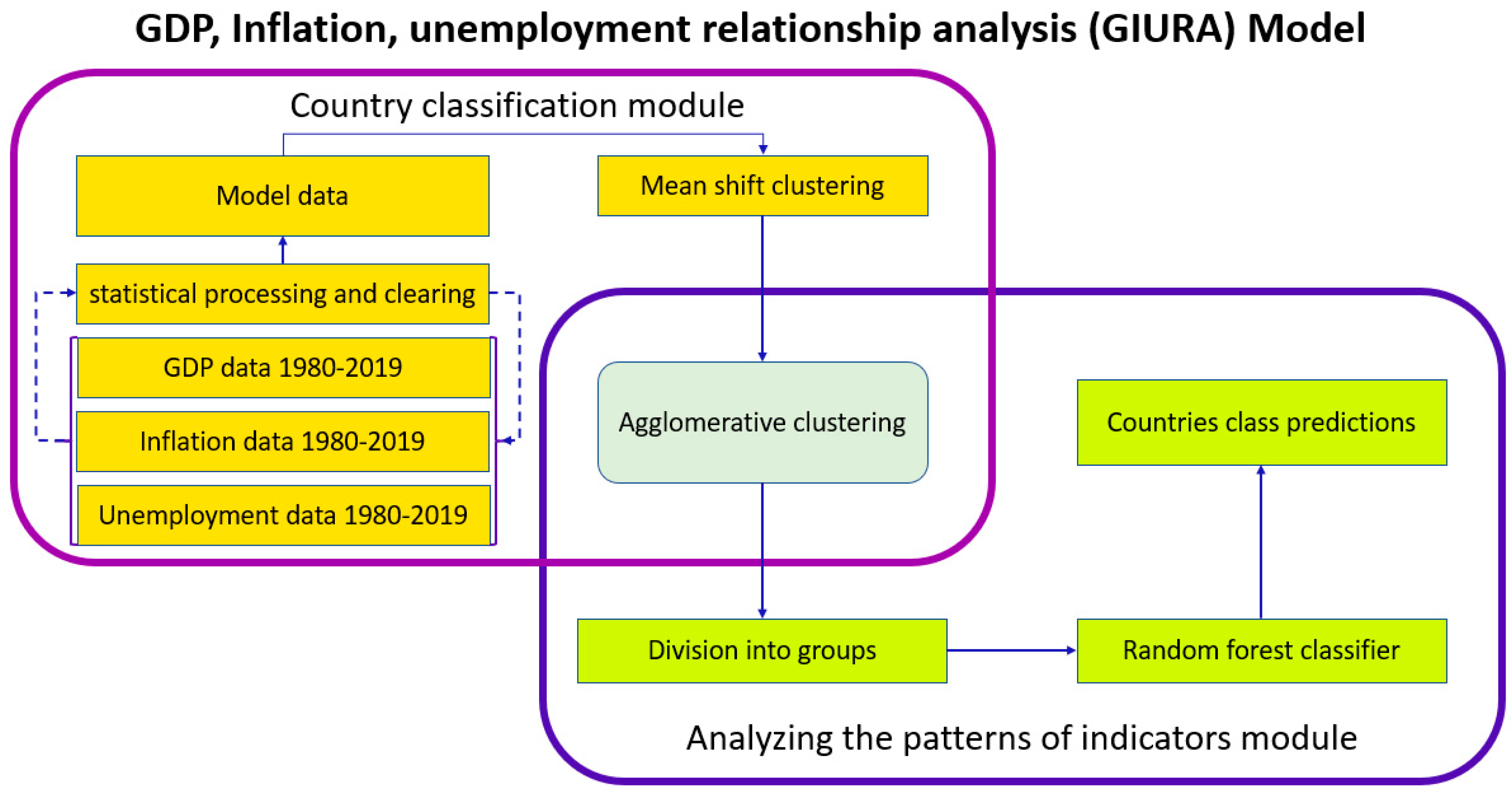
The ratio of the number of features to observations was excessive (90/115 is not suitable for the correct operation of machine learning algorithms without a teacher). Hence, after a rough estimate and calculating the required number of samples, 9 features were compiled for each observation. For this, according to Juglar’s observations, a table of the average level of indicators was formed with a step of 10 years for each of the countries for the period 1990–2019. In general, this and subsequent stages of data processing and model creation can be displayed graphically (
Figure 1).
As can be seen from the image, after the described processing processes, the first stage of applying machine learning follows, in particular, the clustering algorithm for shifting to the mean. The advantage of this approach is that it does not require the input of a certain set of classes or their form; that is, it independently determines the number of formed groups, which is why it was chosen for the primary grouping [
72,
73,
74].
The principle of operation of this algorithm is to estimate the kernel density. For explanation, assume that there is a dataset n of data from points {
ui} in d-dimensional space. Let the kernel
K with the bandwidth
h be selected. Then, together with the kernel function, they form an estimate of the kernel density distribution:
The designations described in the previous paragraph remain the same for the subsequent formulas of this section.
Directly, the shift-to-mean algorithm uses this estimate to shift the suspended particles in the direction of higher density. The kernel function must meet the conditions:
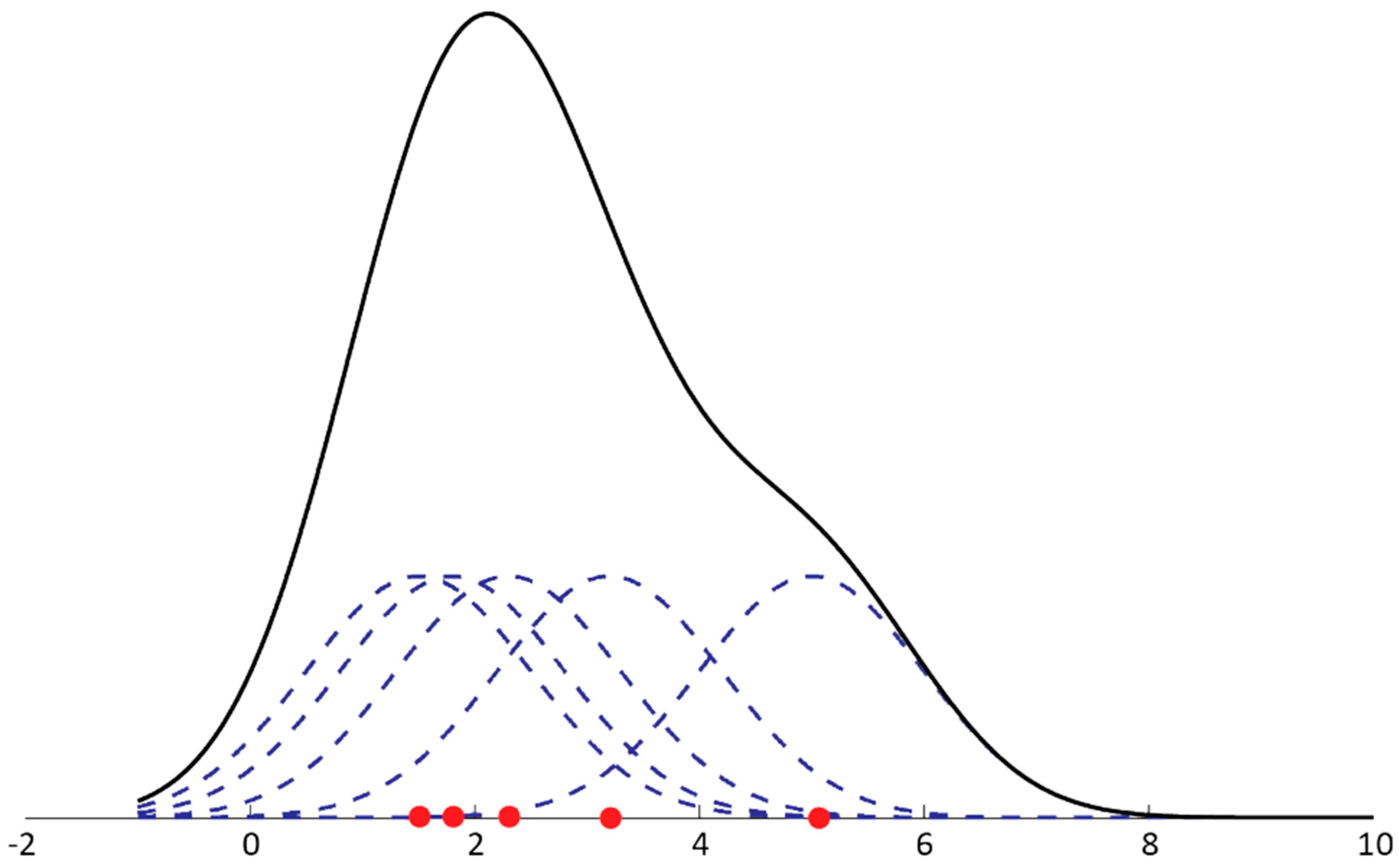
The first condition is necessary to check the normalization of the estimate, and the second is related to the symmetry of space. For the study, a Gaussian function was used that satisfies these conditions:
This is easy to imagine in a one-dimensional data space, where a small (dashed blue) curve is estimated for each new observation, and their increments are added and create a total estimation curve (black); the principle of the algorithm is then clearly visible on the graph (
Figure 2).
Then, it turns out that directly, the shift-to-mean algorithm uses the above estimates to determine the direction of the shift of the suspended particle in space (the initial data in d-dimensional space) in the direction of increasing density. In this case, the principle is similar to the gradient and takes the form:
where:
In other words, m (u) is a vector, called the mean-displacement vector, that determines the direction of increasing density where the points should move. Simplifying, the principle of the Mean Shift algorithm can be described by repeating the following chain of actions:
Calculation m(ui) for each ui
Movement of all ui in ui + m(ui)
Clustering by this method ends after all the initial data have been distributed over some points of data accumulation. Often, to explain this principle of operation, developers use a “gravitational” example: when a certain number of small particles are distributed in a closed space with cosmic conditions. After some time, some of them will collide and create an area with relatively increased gravity, which will continue until all the particles are collected in a number of large objects.
As follows from the first graph describing the model, at the second stage of data classification, the agglomerative clustering algorithm was used. In the work, we used its hierarchical variation: that is, according to the method of combining “from the bottom up”, graphically it looks like a tree structure. All observations are specified first as single-element clusters, then they are combined according to the set criteria. This process is repeated until the end point or the specified number of clusters is reached.
The final stage of data mining was the creation and training of the classification algorithm. It will allow you to evaluate the model and classify the countries that were not included in the study. The very idea of the random forest algorithm is to apply a large number of classical tree-like decision-making structures. This helps one to achieve high accuracy without retraining. The decision forest is an ensemble algorithm, which means that it consists of many decision structures of this kind [
5,
50].
The fundamental novelty of the methods used in this work is primarily in the sequential combination of the above-described clustering methods. They organically complement each other due to different approaches to the selection of groups. So, mean shift in the presented model is indispensable for the initial assessment of the feature space and in determining the possible number of their groups. Agglomerative clustering at the second stage acts as a more accurate clustering method that allows you to combine countries into the number of groups obtained by the estimate from the previous method. The Random Forest Classifier method completes the described model. It allows you to define in groups countries that were not included in the study. Additionally, this algorithm makes it possible to evaluate the importance of each of the features and determine the fairness of their ranking, which will be investigated in the next section [
16,
17].
All of the above transformations are a major part of the work and serve the purpose of clustering. To validate the results, random forest regressor methods will be used, and many statistical measures will be used to evaluate the forecast series and classifying algorithms. In particular, the regression random forest has exactly the same principle as the classifying one, and the main difference is already the interpretation of the results in the form of vectors of the obtained values. The indicators were selected to assess the quality of the models. The following will be used for indicative regression: RMSE stands for Mean Squared Prediction Error; lower is more accurate. MAPE stands for absolute percentage error; lower is more accurate; DAR stands for Directional Accuracy Ratio; higher is more accurate; which are calculated by Equations (7)–(9):
In all Equations above:
yi is the real price value at i moment of time;
ŷi is the forecasted price value at i moment of time;
n is the number of forecast values compared to real data;
d = 1 if (ŷ − yi − 1) (yi − yi − 1) > 0 and d = 0 otherwise.
In general, external metrics are used to verify the quality of clustering–evaluating the compliance of the obtained groups with previously known ones, and internal ones are based only on available data. Since one of the goals of the article is to propose new methods for grouping countries, more attention is paid to internal indicators, and for external ones, a comparison is used between the compiled model, but with other settings. So, two external metrics of variation of information and purity were chosen, and from internal metrics [
26].
VI is a measure that measures the loss and acquisition of information during the transition of observations between clusters. Technically, an indicator represents a measure of the distance between two clusters. Its values almost reflect the level of importance of individual observations for their clusters:
Hereinafter, , , , where i, j are the row and column numbers in the conjugate table, ai is the sum of the table row, bi is the sum of the table column, nij and xij are directly observations or cluster elements, n is the sum of all table elements, ckl is some cluster, dps (xi, ck) is the symmetry distance of the xi point of the cluster ck, M is the number of clusters,
The second external metric is purity, which maps the largest class in this cluster to the cluster. It is in the range [0, 1], where 1 is the best clustering option and the figure is calculated according to the Equation below:
The first two internal indicators WSS and BSS characterize different sides of the same property of sets of observations–distance. The idea of the first indicator is that the closer to each other objects within clusters are, the better the separation, which means that the intra-class distance, in particular, the sum of the squares of distances, should be minimized. BSS is the opposite in its idea, since this metric considers the distance between different clusters, and the larger it is, the better the distribution; therefore, the task is to maximize the sum of squares of deviations. Both figures are calculated according to the Equations below:
The remaining indices are more complex to interpret into reality. Sym evaluates the entire data set and formed clusters at once, which makes it useful in validating models, and the main task is to maximize it. Physically, it displays the relationship of the clusters defining the set and their symmetries. Calculation is performed as follows:
Completing the selected collection of clustering metrics is the Silhouette model. This indicator is needed to assess the “similarity” of clusters among themselves. All cluster structures are evaluated according to the Equation:
where the key complexity is the numerator. It looks for the difference between separability: that is, the average distance from
xi∈
ck to objects from another cluster
cl:k ≠ l, and compactness: that is, the average distance from
xi∈
ck to other objects from the cluster
ck. Separability was found by the Equation:
Compactness is as follows:
The measure itself lies in the range [−1, 1], and a larger value corresponds to a better model.
In order to check the out-of-sample forecast performance of the model, the paper uses the naïve random walk model [
5,
18]. It is well represented by a univariate unobserved component of a time-varying trend model. Previous researchers found that the clear inflation forecasting performance of the random walk model [
6,
14,
15]. The paver uses a Normal–Inverse Wishart prior. In this study, it shrinks such that the model’s parameters are towards a naïve random walk model with time lag:
Later, the paper uses Inverse Wishart prior for the covariance matrix of the residuals. The distribution of the autoregressive coefficients, conditional on the covariance matrix of the residuals, is normal with the following mean and covariance.
4. Results
This section will explore the principles of interrelation of the used open innovation indicators for each of the groups of countries. First, it is worth familiarizing yourself with the groups of countries created by the algorithms (
Figure 3).
Countries are marked in gray for which there is not enough reliable data for the selected period. The classification in the case of Armenia, Bosnia and Herzegovina, the Dominican Republic, China, Kosovo and the United States of American was no longer carried out by clustering algorithms, but by a trained classifier. With the help of this data, the performance of the predictive classifying model will be demonstrated later. For greater accuracy, the data are also duplicated in
Table 1.
To check the validity of the selection of these groups, various statistical indicators will be presented below. Later, a comparative analysis of graphical interpretation of the behavior of open innovation variables for each of the groups will be carried out. Thus, the main set of statistical indicators of variation is presented in
Table 2.
The table clearly shows which factor was decisive for the selection of each of the groups. It also shows the direction and strength of the relationship of indicators. So, for the first three columns (Average changes), the most important for the study of relationships will be the sign (direction) of the average change of a certain indicator, and the order (the number of degrees 10 when the number is presented in standard form). Thanks to these indicators, for example, it can be argued that in group 1 there are countries with rapid open innovation development (the highest average GDP growth) and a competent policy of control over employment (on average, unemployment in the group decreased from 1990 to 2019). The second and third three columns (Average linear deviation, Standard deviation) have a similar meaning, displaying average deviations. The advantage of sequential analysis of linear and standard deviation is the ability to compare the orders of numbers of selected indicators. So, if the difference in the value of the indicator with linear and standard deviations is not large, as, for example, in the growth of open innovation indicators in the 6th group, this means that the group for this indicator is quite homogeneous, and, accordingly, on the contrary, with a large difference, in the group there will be high variability.
To begin with, it is worth understanding the technical veracity of the findings. Strictly speaking, any classification of data sets into groups is carried out in the axiomatic field of clustering algorithms, which gives them a greater level of formalization.
This also made the approach to group formation more creative and weighed down the choice of acceptable model statistical validation metrics. However, for the first - mathematical stage of model verification, six indicators were selected, their characteristics and calculation methods are in the section "methods" for Equitation 10-15. The results are shown in
Table 3.
From the obtained values and based on their interpretation, described in the section “methods”, it can be concluded that the purely statistical and mathematical side of the implementation is quite suitable for further study. Now, it is worth interpreting the results in a practical economic field.
A key prerequisite for compiling their own unique classification of countries was the assumption that this could increase the predictive accuracy of machine learning models for the group of indicators in question. A regression machine learning algorithm will be proposed to test the applied benefit of the proposed country separation. It will be built on the same data, but with different predefined input weights (indicators of the importance of certain data). In particular, 3 sets of data on the 3rd studied open innovation indicators for the selected period (GDP, inflation, unemployment, 1980–2019) were formed, characterized by the following features (hereinafter, the work will be reflected as data types 1–3, respectively):
- (1)
Entering “clean” data without any processing;
- (2)
Bringing the data to increase values (statistical processing methods used in the work are described in the section “methods”);
- (3)
Pre-processing and splitting of training sets according to the selected groups.
The results will be presented in tables and are based on examples of countries of some groups immediately after consideration of the dedicated clusters.
Table 3 allows you to visualize the relative importance of each of the characteristics in the distribution of countries into groups, which is very important for assessing the adequacy of the classification. Based on the histogram, it can be seen that the largest difference does not exceed 8%, which means that the selection of countries by groups involved data on all 3 open innovation indicators for the entire selected period of time 1980–2019,
Figure 4.
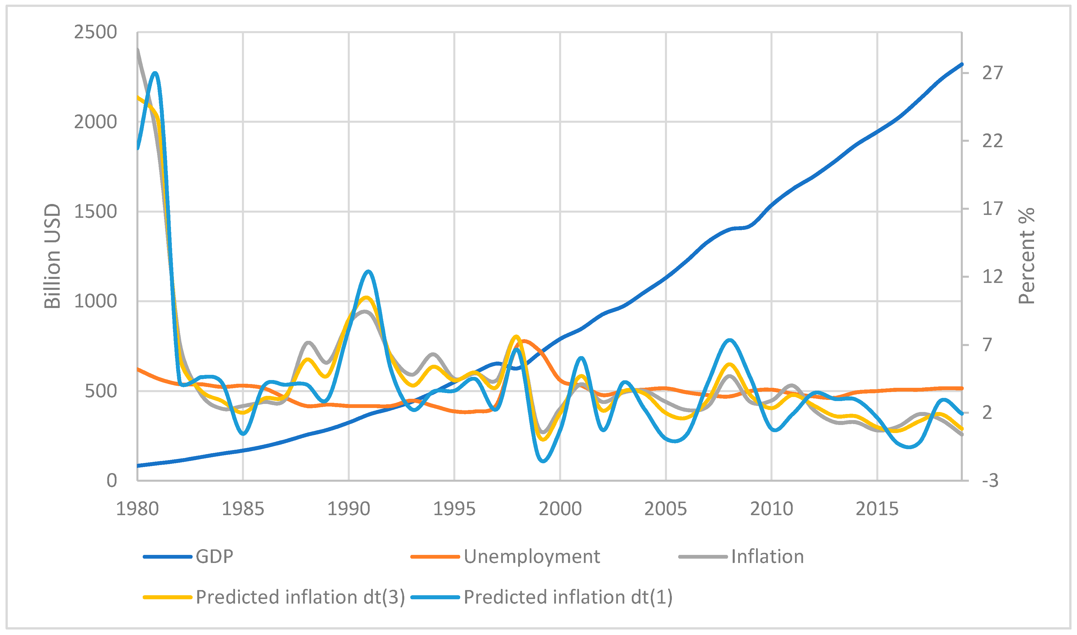
In this group, it was decided to test the intended practical benefit of the proposed clustering on the example of South Korea. Such a choice was made in order to immediately eliminate the neglect of classification based on the high heterogeneity of historical, political and geographical characteristics of countries belonging to different groups. The table thus shows different results of the simple forecast model described in the section "methods" for Korea (
Table 4).
As can be seen from the presented table of variation metrics, the quality of inflation forecasting even by simple methods increased almost 2 times in comparison with the usual analysis of time series, and almost 1.5 times in comparison with data trained in other classifications of countries. The change in the quality of forecasts using different methods is presented in
Figure 5:
It is worth noting that when applying the proposed methods, both the exact determination of trends and their strength improved, which increased the overall forecast strength by 30%.
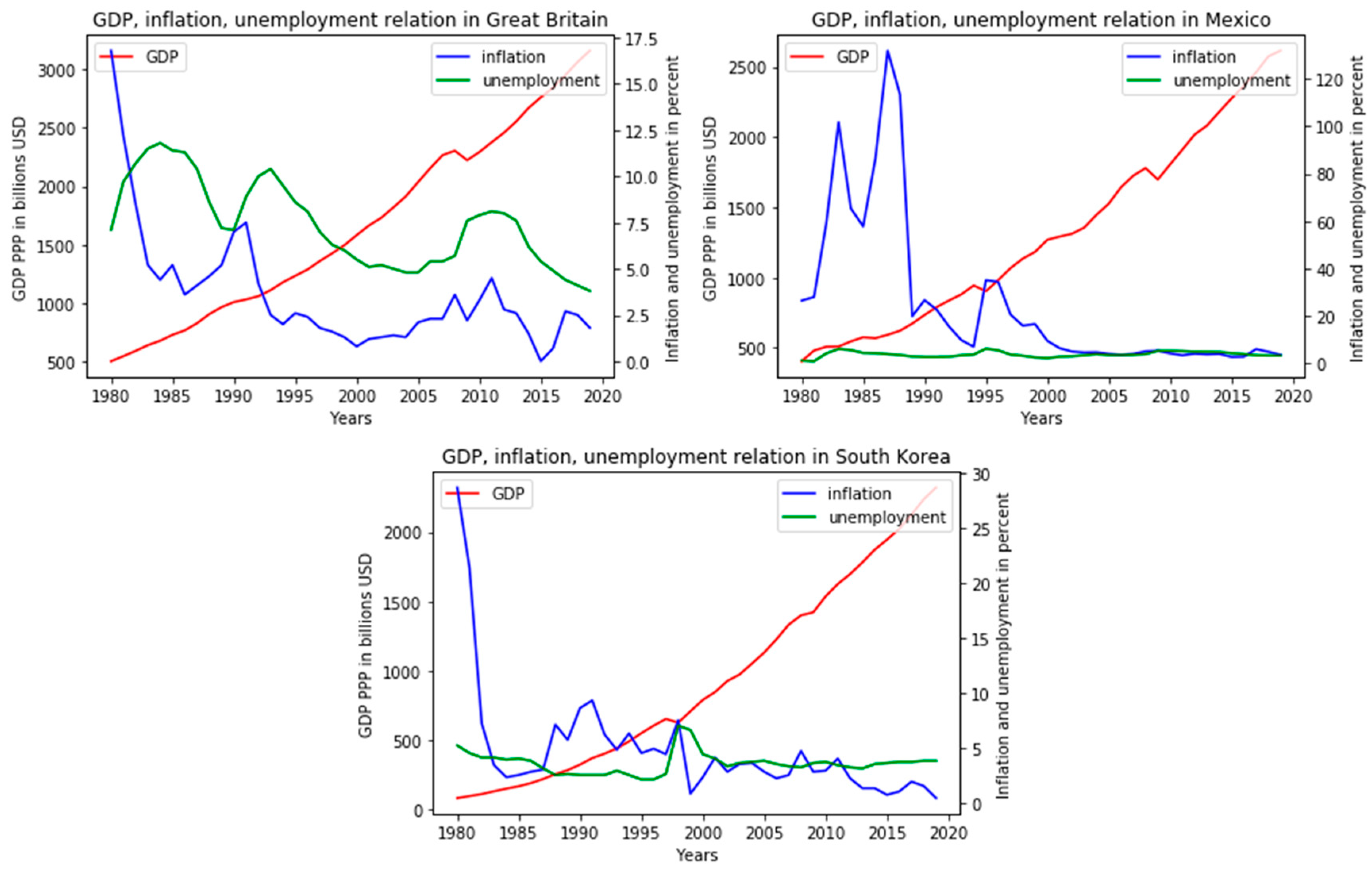
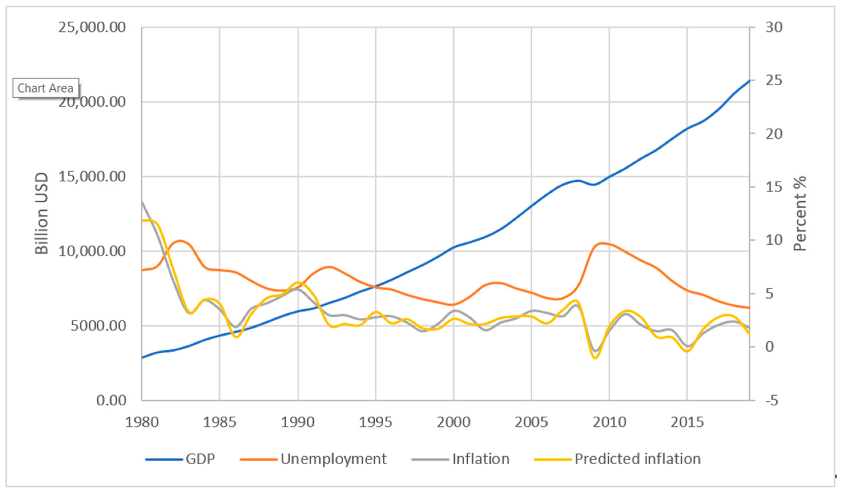
In addition, the first group was supplemented by countries excluded from the model-building data: USA and China, so it is advisable to immediately compare their graphs with the main group,
Figure 6.
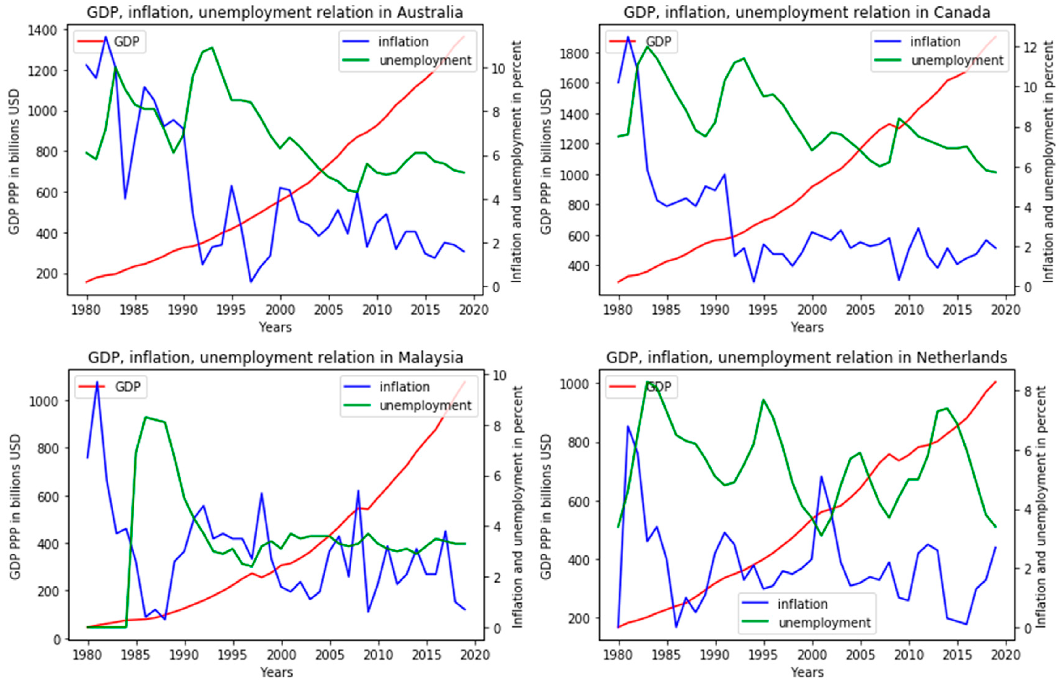
On the whole, we can conclude that the general trend was identified quite correctly. It is also worth highlighting that the countries that were developing in the 1980–1990s are experiencing strong surges in inflation, especially among Asian countries. The tendency towards a direct relationship between inflation and unemployment, but their inverse proportion to GDP, becomes obvious. It is noteworthy that this group includes mainly developed countries. As another feature, we can highlight the weak validity of Phillips’ statement on the data of this group, since the inverse proportionality of unemployment and inflation is found in only a few places in the graphs, and the opposite is much more common. In the UK, these indicators generally demonstrate a direct relationship with a small difference in levels, so it is fair to say that for countries with such a relationship of indicators, traditional methods of finding relationships are not relevant.
It was decided to carry out a similar practical validation for the United States of American, taking into account the predicted class. Despite the addition of possible algorithm errors, the overall accuracy of predictions using group-differentiated learning still increased, which can be seen from
Figure 7, above, and
Table 5, below.
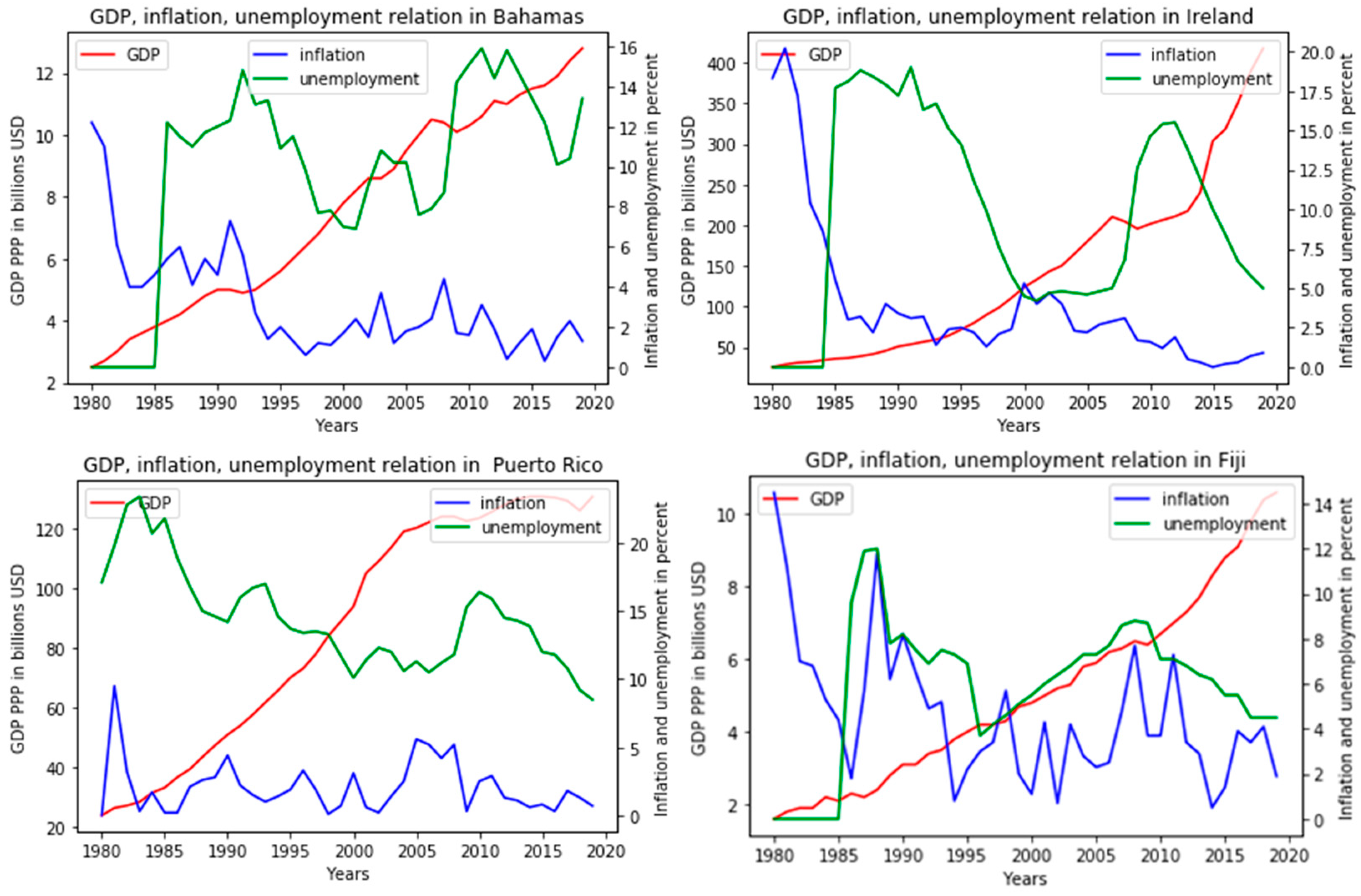
The second group is characterized by sharp peaks of inflation up to a certain period. After passing a critical point, this process calms down, and unemployment becomes consistently higher than inflation by several points. In this group, there is no classical unity according to the geographic or political criteria of generally accepted classifications. This includes both countries with a so-called developed market economy, countries in transition and even developing countries, with different political regimes and specialization of the economy, but the described pattern is valid for the entire (
Figure 8).
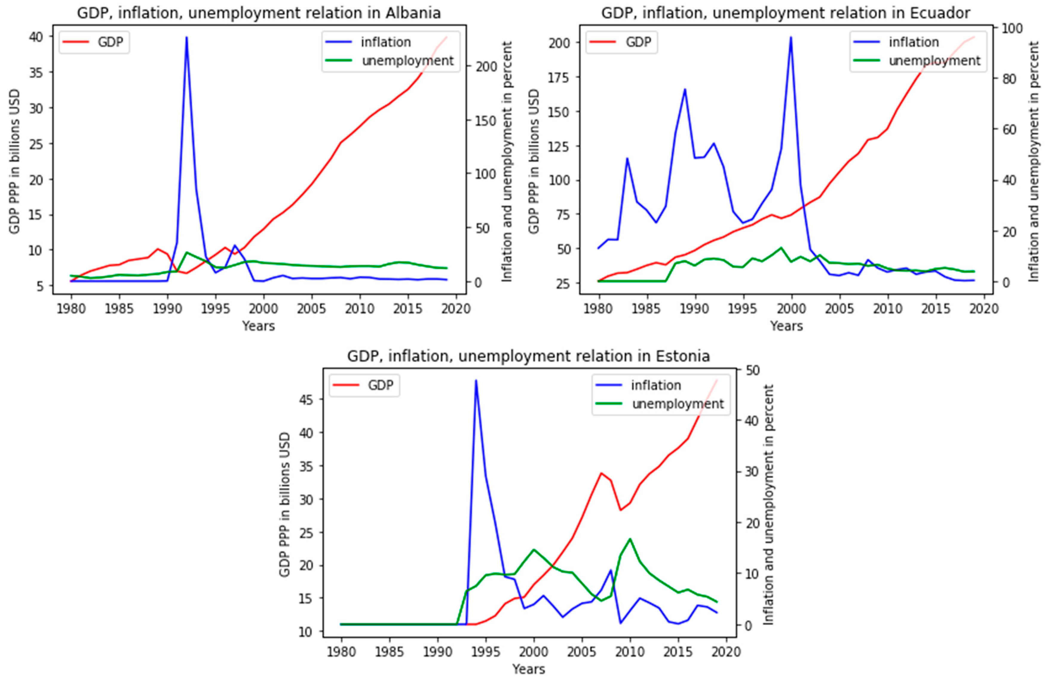
For the analysis of the third group, two countries were selected. This was done for greater clarity, since in Belarus, Russia and Brazil, the structure of the behavior of indicators is very similar, but at certain times of crisis, inflation went off scale to thousands of percent, which hindered clarity. The third of the graphs for this group are the approximate values for Belarus. In this group, the patterns described by Phillips are practically not traced. Additionally, if we compare with the first group, in the comparison of inflation and unemployment, the opposite trend is observed, and inflation is consistently higher. In general, countries with high economic instability were included in this group; classical normative theories are also not suitable for analyzing their indicators. The indicators themselves are presented in the graphs (
Figure 9).
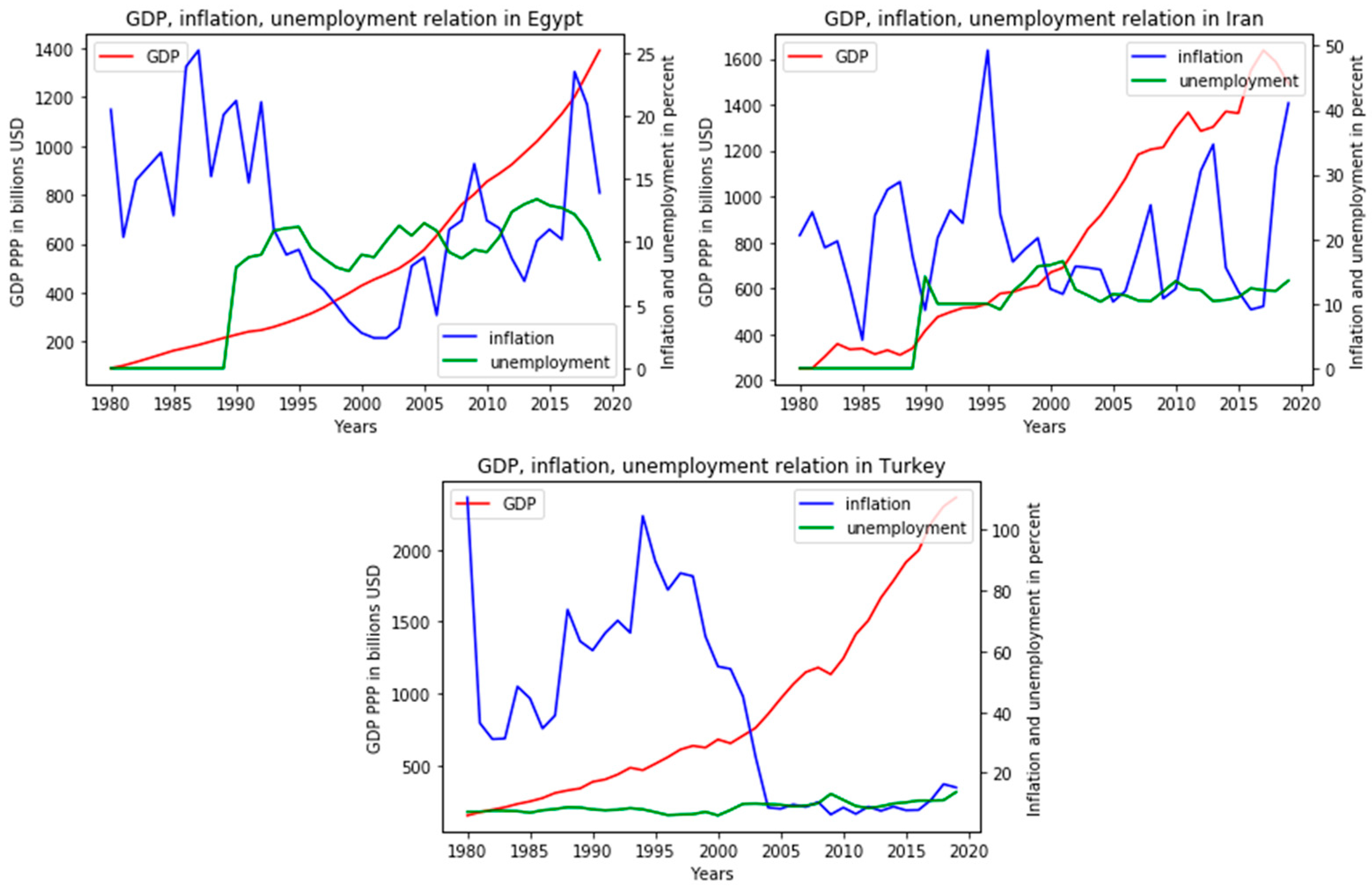
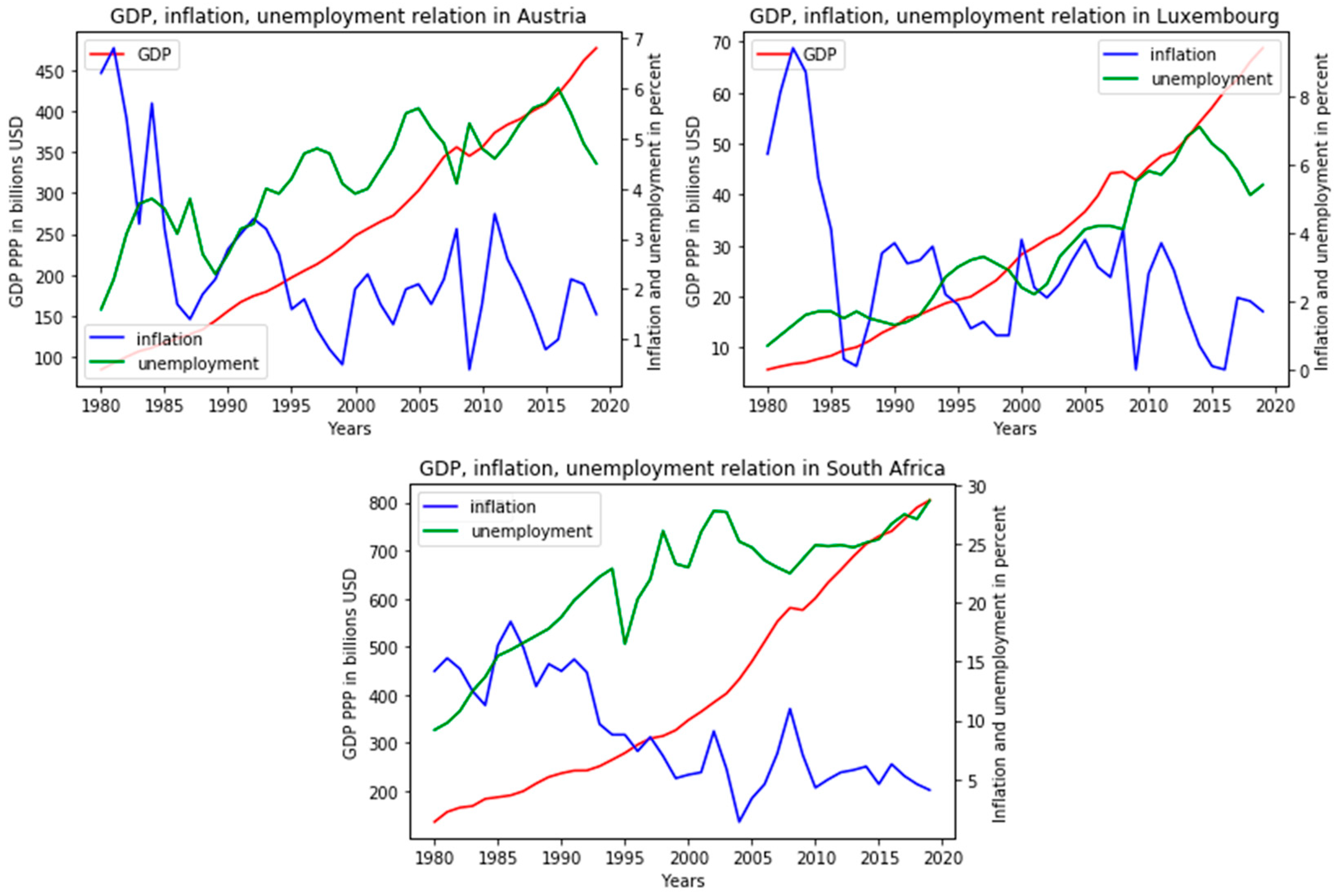
Most of the states from the fourth group are located geographically close. From the point of view of the presented model, getting to them is explained by the similarity of indicators, and from the point of view of classical methods of open innovation analysis, all states of this group have similarities in historical economic cycles and prerequisites for development. The indicators presented in the graph below also allow us to conclude that the usual interpretation of the Phillips curve is not fulfilled for these countries. Inflation has a spasmodic appearance with periods of peaks of several years, and unemployment changes from directional and less dramatic (
Figure 10).
It was decided to make an early practical test for this group of countries with high inflation variability during the period under review; the test results are presented below in
Figure 11 and
Table 6.
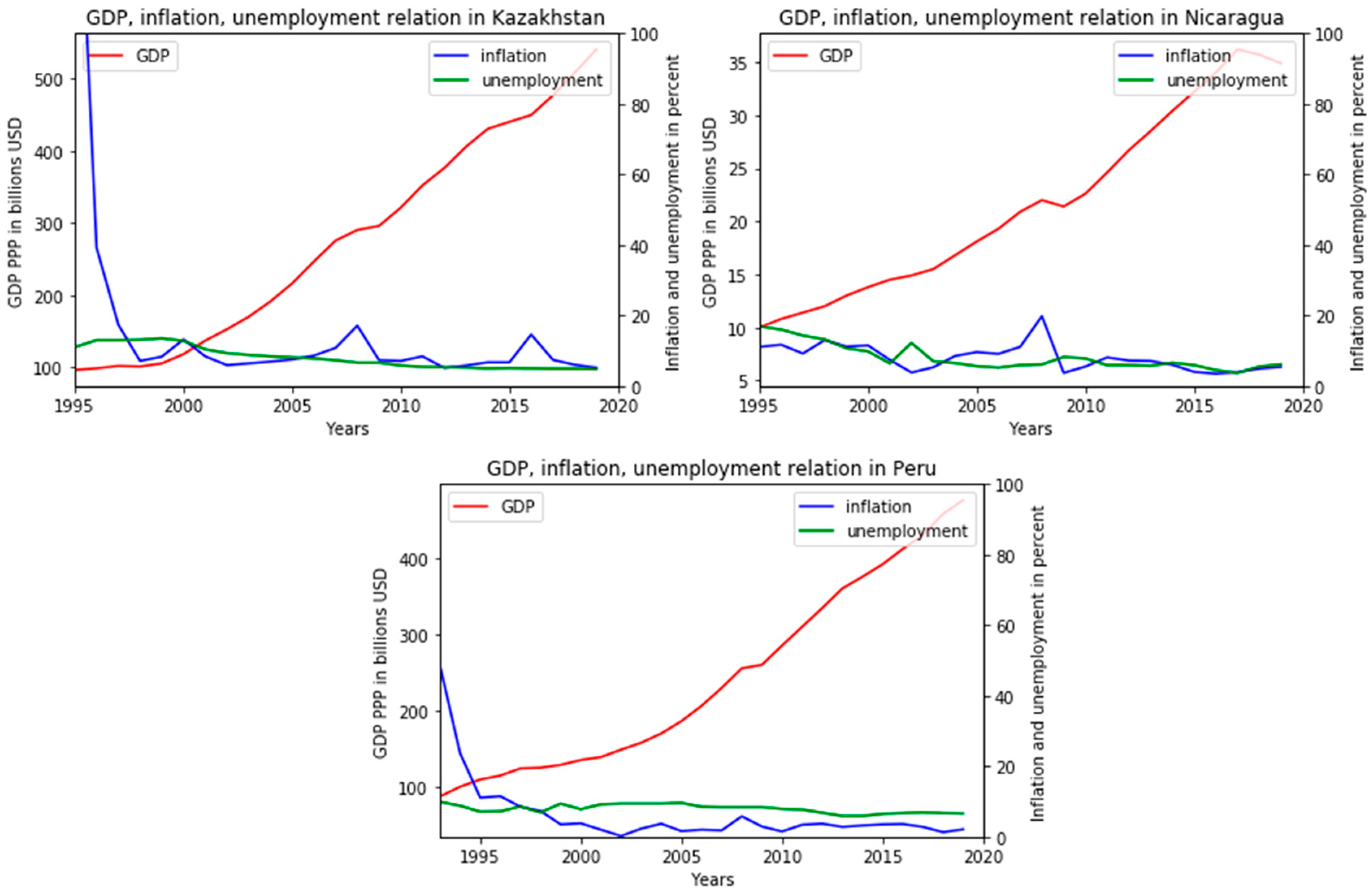
The fifth group is the most numerous: that is, out of 114 countries suitable for analysis, the trends encountered here will be the most common around the world. In terms of the relationship between GDP and unemployment, this group is similar to the previous one. The main difference from what was previously encountered is the likelihood of the Phillips curve. Thus, the graphs show that inflation peaks (highs/lows) occur at the same time as the opposite peaks of unemployment (lows/highs). It can be noted that the general trends in these indicators are also multidirectional, and unemployment in the countries increased over the period under review, although inflation decreased, which indicates the fulfillment of the Phillips law for these countries in the long run. Due to the size of the group, and, consequently, the prevalence of the traceable patterns of connection between indicators, this group most obviously casts doubt on the currently available classifications of countries, on the basis of which, forecasts and conclusions are then built, as can be seen from their descriptions above and the following graphs (
Figure 12).
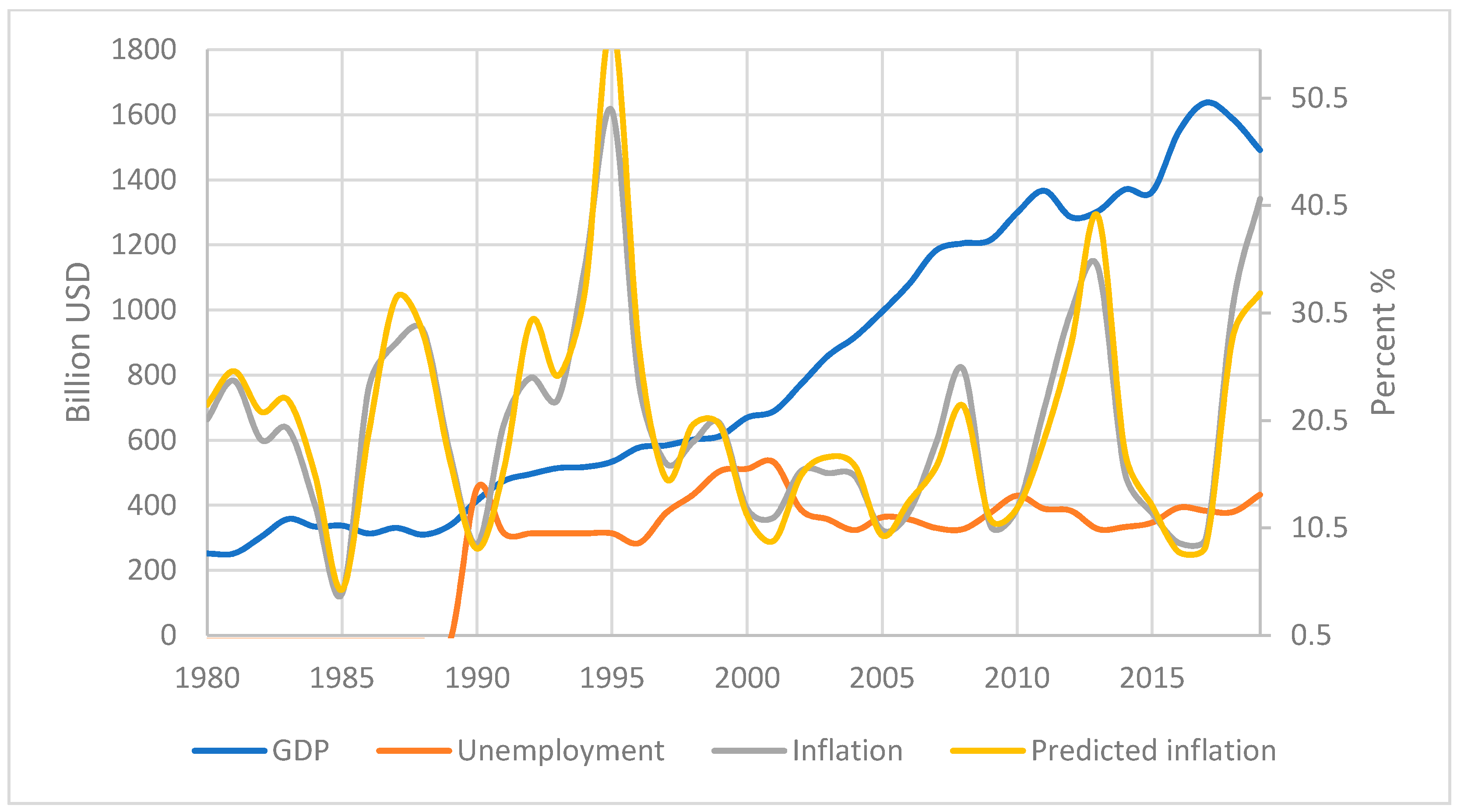
The indicators of the countries of the 6th group will change quite distinctively. All of them have seen a sharp jump in inflation for the period 1990–1995; therefore, to improve clarity, that period was partially shortened so that further inflation and unemployment data would not approximate the zero line. The pattern itself for these countries is quite simple: slow linear GDP growth, with small retreats during periods of political or economic instability; relatively high inflation rate, which, however, is inevitable for a developing state; periodicity in a spasmodic rise in inflation of about five years, which corresponds to the Juglar cycle; stable and fairly low unemployment rate, which was confirmed by
Table 2,
Figure 13.
The most normative behavior of open innovation indicators of countries, from the point of view of the theories that formed the basis of this article, is observed among these countries of the 7th group (
Figure 14).
In this group, there is a fairly typical pattern of downward changes in inflation and unemployment in comparison with the growth of open innovation indicators, which, and the ideas of Phillips and Okun remain valid. For most of the period under review, with a decrease in unemployment, inflation increases in countries: that is, the minimums of one indicator are located approximately below the maximums of another, and vice versa. At the same time, Okun’s ideas are being fulfilled, and it turns out that when the GDP curve becomes flatter, unemployment begins to grow at about the same time.
The final eighth group includes 11% of the studied countries. This group is also largely controversial from the point of view of classical views. It will definitely not be possible to single out the pattern of connection of indicators for these countries using traditional methods; we can only state that the ideas of Okun and Phillips are valid only in some cases and no longer than in the medium term. Thus, the graphs show that the inverse proportionality of unemployment and inflation explains only a small part of the data movements and no longer than on a horizon of several years (
Figure 15).
First, the validation of the GUIRA model to naïve random walk model (NRWM) includes the inflation rates, unemployment and GDP of the 10 largest countries. The task is to clear whether the information provided by key drivers is valuable to predicting parameters.
The paper used vector auto regressions to measure uncertainty in this paper as in previous research [
70]. As a result, it is important to at least summarize the estimates of the a posteriori parameters and what implications they have for inferences such as impulse response functions. In this paper, we derive a machine learning model based on the principles of shift to the mean, agglomerative clustering and random forest methods. Using these methods, this paper classifies countries according to the level of open innovation implementation and the values of macroeconomic indicators into three categories, each of which contains its own sets of parameters. The analysis shows that the proposed algorithm has a higher computational efficiency than the random walk model. The hierarchical algorithm proposed in this paper can combine other mathematical tools. The results presented in
Table 7 are, in fact, out-of-sample forecasts. The paper used the sample to estimate the parameters of each model. The author(s) adopted a Bayesian approach for estimation of the naive random walk benchmark, like previous searchers [
71,
72,
73].
The authors used the results of previous studies for a vector auto regression (VAR) set up. The authors also use a multi-variate set up for the benchmark like previous searchers [
55,
56]. The paper includes a literature review on the variables in the model and the stationarity/transformation with macroeconomic indicators. If it is the latter, then this is the incorrect prior to use. The results show that the GUIRA model has higher predictive power than NRWM (
Table 7).
The evolution of return interdependence between GDP, inflation, unemployment is derived by means of time-varying parameter copula models. The interdependence measures obtained are used in Bayesian vector auto regression (BVAR) models with the Litterman/Minnesota priors and local projection to quantify the responses of the GDP and macroeconomic indicators [
70,
71,
72]. The BVAR model with the Litterman/Minnesota priors is prepared especially to manage with the over-parameterization of VAR models [
72].
A fairly long period of time of 30 years was used in the study; most of the currently existing countries from all parts of the world were involved, so some intermediate result can be summed up. From all the data presented, it can also be inferred that the classical assumptions about universal open innovation laws are largely outdated or in need of a very strong correction. In addition, the graphs clearly show that regression models should take into account the time biases in relation to indicators.
5. Discussion
Before comparing the results with well-known works, it is worth resolving some general theoretical differences. First, changing approaches to measuring and understanding indicators during the period under review does not have a significant impact on the results, since the statistical processing technique used breaks the data into related blocks of 10 years, and over this period of time, the changes are not so critical. Secondly, the same applies to related indicators on the type of interest rate, labor market characteristics.
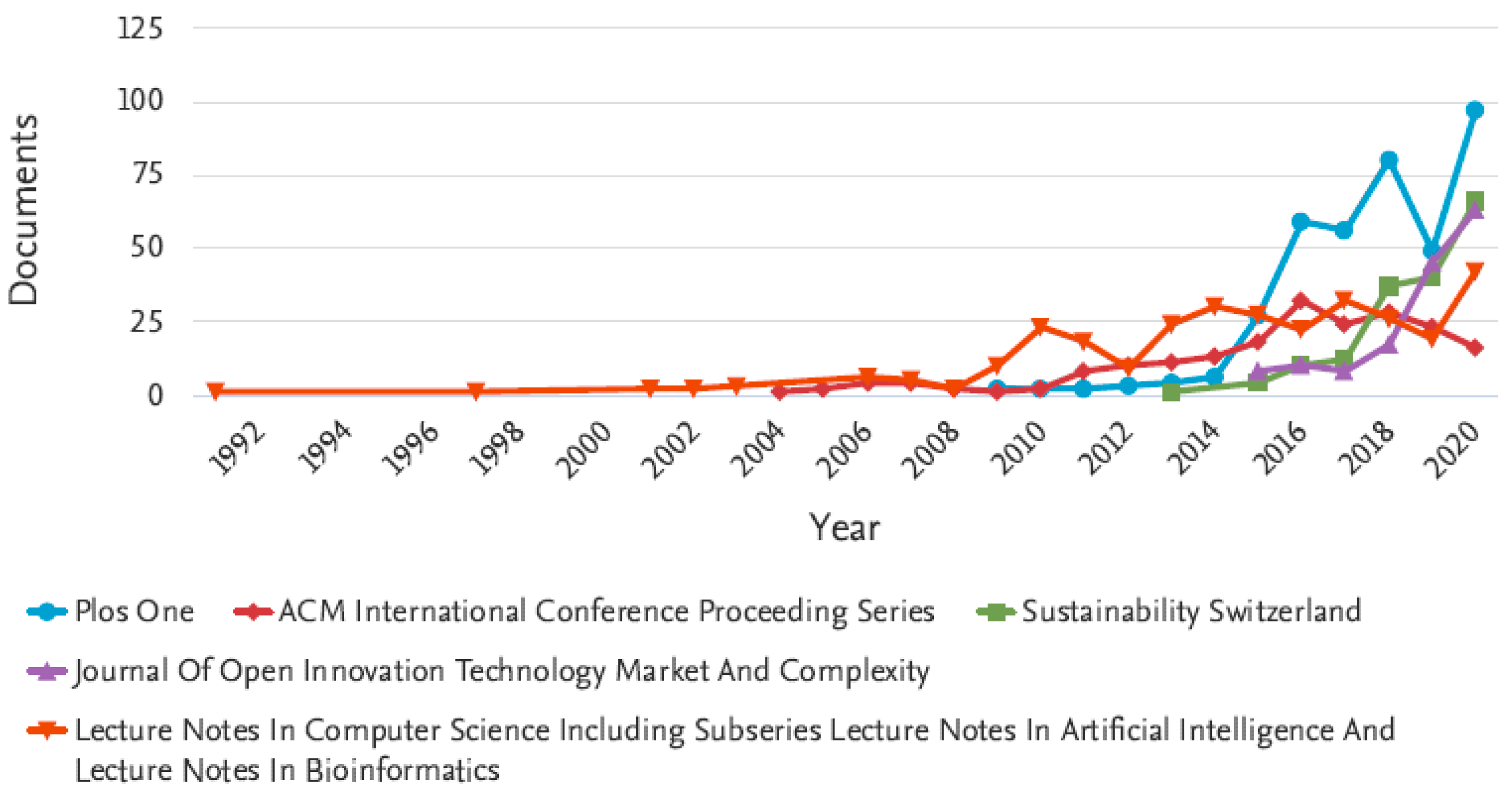
Many researchers around the world studied the diffusion of open innovation from 1992 until 2020. In 2018,
Plos One Journal had the highest quantity of research in this field. These initiatives are aimed at cooperation between participants of open innovation and implementation of the principles of open innovation. Based on large-scale innovation survey, the authors compared open innovation in private enterprises with the same in state local companies. Our data confirm the bidirectional causal relationships between open innovation and economic growth. This idea is approved by Open Innovation dynamics of keywords in top journals (
Figure 16).
Technological level of the production sector of the global economy, which was formed at the beginning of market reforms, it cannot be considered progressive and corresponding to the level of developed countries [
74,
75,
76,
77,
78,
79,
80,
81].
Of course, having obtained such a result, one could refer to the exceptional fidelity of the Friedman-Phelps concept, which assumes the absence of long-term strength in the Phillips curve. In addition, their conclusion is quite consistent with historical logic and a departure from Keynesian ideas, but even in this case, everything is not completely clear [
82,
83,
84,
85,
86,
87].
They tried to question Phillips’ concept, but used methods similar to him, which did not allow them to overcome the fundamental discrepancy between the object and research methods. In addition, the result achieved by them can be refuted even by empirical methods, for example, by looking again at the data of the seventh group from the previous section, where Phillips’ ideas remain partially true in the long run. Economist Robert Lucas also developed the idea of the final determination of the relationship of the factors under consideration. He has already changed some methodological approaches, and began to study inflation expectations in the economy, as a result of which he came to the conclusion of a sufficiently high explanatory power of the Phillips model in the short term, but the need for significant refinement and customization for the purpose of the study when trying to apply it over a long period of time [
88,
89,
90,
91].
This work agrees with the last conclusion to a greater extent. The key differences of this work from the existing ones are approaches to data preprocessing and variability of methods. This has been described in greater detail in the “methods” section, but when compared with other studies it is worth clarifying this again. Thus, the novelty of the methodology consists in combining different economic doctrines. In this case, classical open innovation views were checked, and to assess the set goal, the data were processed according to some methods of marginalists, in particular, to analyze the behavior of data in dynamics, the idea of assessing the absolute change in indicators over periods of time was used. This makes it possible to accurately take into account the behavior of factors in the model and not discriminate in scale [
92,
93].
Thus, the discussion includes the novelty of the research results in the next fields:
(1). Introduction of an objective model to measure open innovation and its application to the information technology convergence sector.
(2). The role of strategic orientation.
(3). The effect of open innovation on technology value and technology transfer: a comparative analysis of the automotive, robotics, and aviation industries.
(4). The role of openness in explaining innovation performance among U.K. manufacturing firms.
(5). Entrepreneurial cyclical dynamics of open innovation.
(6). How firms dynamically implement the emerging innovation management paradigm.
(7). Micro and macro dynamics of open innovation with a quadruple helix model.
(8). How open innovation is enacted in paradoxical settings.
(9). The culture for open innovation dynamics.
6. Conclusions
In this study, the generally accepted methods of classifying countries and the inherent ways of modeling their open innovation indicators were questioned. For this, various statistical and programmatic visions of data analysis in economics were used. With the help of this approach, it was possible to show the inconsistency of the current modern classifications of countries, and also to propose our own. The main advantage is the specificity of the selected indicators, their economic, political and social nature, which gives a reflection of various vital aspects of the existence of states. This result proves that an analysis based on the behavior of open innovation indicators, which are complex in nature, gives a more complete picture of the life of states than valuation models, such as, for example, the development of market relations, development indices, political relations and others.
For more accurate future models and classifications, researchers are expected to select consistent metrics that encompass fundamental patterns explored by the social sciences. This approach slightly complicates the models and concepts themselves but allows one to significantly improve the quality of analytical groups and the accuracy of predictive calculations for different blocks of states. In this article, based on mathematical approaches in economic modeling with elements of machine learning in the python language, a country clustering model is proposed. This allows us to state at least three areas of the contribution of work to the development of the body of available knowledge in the social sciences. Firstly, for the analysis, it is supposed to use changes, that is, increments over equal periods of time, data and not directly their levels. This allows one to find non-obvious similarities, regardless of the size and current development of the country. Secondly, the created econometric model allows the building of regression models and forecasts for groups of countries on its basis or using similar ideas to create other classifications. Thirdly, the main achievement of the work can be considered the proposal to change the established ideas of groupings of countries by blocs.
To increase the accuracy of this approach to identifying groups of countries based on open innovation indicators in future studies, researchers can use a vector model, but it is a little more complex and requires more time to train. The next researchers can also take a lot of datasets for all years with all the other macroeconomic indicators.


