Design Trend Forecasting by Combining Conceptual Analysis and Semantic Projections: New Tools for Open Innovation

Abstract

In this paper, we describe a new trend analysis and forecasting method (Deflexor), which is intended to help inform decisions in almost any field of human social activity, including, for example, business, art and design. As a result of the combination of conceptual analysis, fuzzy mathematics and some new reinforcing learning methods, we propose an automatic procedure based on Big Data that provides an assessment of the evolution of design trends. The resulting tool can be used to study general trends in any field—depending on the data sets used—while allowing the evaluation of the future acceptance of a particular design product, becoming in this way, a new instrument for Open Innovation. The mathematical characterization of what is a semantic projection, together with the use of the theory of Lipschitz functions in metric spaces, provides a broad-spectrum predictive tool. Although the results depend on the data sets used, the periods of updating and the sources of general information, our model allows for the creation of specific tools for trend analysis in particular fields that are adaptable to different environments.

1. Introduction

Trend analysis and forecasting is an indispensable task in the preparation of projects in almost any field of business activity. For example, it is essential in the planning of new commercial products and in industrial or artistic design. These issues have often been resolved in specific contexts through the expertise of professionals, sometimes using some technical tools that are now well established (GoogleTrends, Facebook Analytics, …). However, there seems to be a certain lack of theoretical frameworks that can facilitate the development of these tasks. It is clear that this is a crucial point for the success of any design project, so any tool that could improve the efficiency of the process would help all the agents involved.

Based on a mathematical structure built on metric spaces of fuzzy sets, and in our practical knowledge—the result of our experience in the field of design and education—we present in this document an attempt to obtain an easy-to-use tool supported by two legs, trying to mix them in a common framework that could be handled by the analyst interested in improving her/his results through a reliable tool. The idea is to produce a new Open Innovation tool, which is proposed as a way to create a common framework for collaboration between design experts in a given industry, and data scientists, mathematicians and linguists, with the aim of developing an Internet-based technology for the analysis of design trends. The result of the collaboration of these professionals would be the creation of a specific forecasting tool in an innovative context.

Let us briefly present the two columns that support our ideas. The first of these is conceptual analysis, which becomes a practical tool in the development of the knowledge structures that are called ontologies—with a standard formal meaning in the context of Artificial Intelligence—by setting categories of concepts and relationships between them. In the words of Fallis [1] (Section 2), “the goal of the method of conceptual analysis is to find a list of necessary and jointly sufficient conditions that correctly classify things as falling under a given concept or not” ([2] (Section 2.1) and [3]).

Having roots in Analytical Philosophy, and Phenomenology in the tradition of Brentano and Husserl, the idea is to organize under a logical scheme a knowledge that can be used to guide inductive arguments in the concrete context for which it is created. Although the main technical developments in this direction were made already in this century, the origin and basis of conceptual analysis was clearly explained by Guarino and other authors in the 1990s. In this sense, in this work, we follow the conceptual framework presented by the author in [4].

A formal environment defined in this way is the starting point of our method. Based on our experience, we defined a general conceptual structure of categories and relations, setting the main axes and subordinate conceptual fields that organize the main design trends today, with the aim of helping designers and professionals in general. Therefore, we have firstly built a conceptual scheme—called Deflexor—that could guide people interested in arguing about the future success of the products in which they want to invest, time, work, effort or also money. All information about can be found in [5].

The second source from which we have drawn our tools are some recent developments in artificial intelligence. Based on the fundamental ideas behind some formal semantic structures known today (ontologies, vocabularies, general tools for the representation of knowledge and engineering), we developed a technical tool that is presented in this paper. We used the central notion of semantic projection on a conceptual universe, which is explained in this document both from an abstract and a practical point of view. Although we intend to define it as a purely abstract notion, the origin of this idea can be found in almost all classical approaches to automatic semantic analysis, being close, for example, to the notion of semantic embedding and representation based on vector space, on which current tools such as Google’s Bert are based.

As we will see, the notion of semantic projection allows us to isolate the way in which a concrete projection is calculated and how a particular universe is defined, from the general theoretical structure of the model. The main idea is that it is possible to generate a series of combined universe+projection structures, which, optimized through the use of reinforcing learning techniques, allow us to obtain a useful model to make prospective about design trends. As we demonstrate in this paper, this provides a second-level support platform by aggregating some Internet tools that have already proved successful; for example, Google products such as Scholar, Trends and Analytics, Facebook Analytics as well as some indicators that we have created based on some instruments for internet analysis that we have experienced in recent years [6,7,8]. Together with the conceptual model explained in the previous paragraph, this completes a trend analysis tool for designers and professionals, as a technological element to facilitate Open Innovation.

In this article, we aimed to facilitate access to understanding of the technical part of the process, motivated by the fact that the blind use of an electronic platform is generally not a good way to use such a sophisticated tool. Therefore, in the first part of the paper we go deeper into the fundamentals of our model, to complete it in the second part with easy examples, in order to illustrate how it works. Some advanced mathematical concepts and results are needed, which are explained after this introductory section. Indeed, motivated by concrete examples but trying to find a useful abstract definition of what a trend is, we characterize such an entity as a fuzzy set of concepts/words/labels, which becomes an element of a space in which we define a metric using a specific rule. Thus, the general model is motivated by examples taken from various applied contexts and some classical tools coming from the topology of metric spaces. The indexes are then real functions that act in these metric spaces respecting some compatibility with the metric, which are called Lipschitz functions. For this reason, we adapt some well-known extension results for real-value Lipschitz functions to metric spaces in which the elements are defined as fuzzy sets, preserving the Lipschitz constant for the extended function (see [9,10]). Although the extension theorem that we use is a classical result of the theory of real functions on metric spaces, this is still an active research topic: related results that have been developed in recent years can be found in [11,12,13,14].

The paper is organized into six sections. After this Introduction, we present in Section 2 some mathematical tools which are needed. In Section 3, we explain the construction of our main reference space, the space of trends and innovative ideas, together with a metric. The elements of such space are fuzzy subsets of a given universe U of concepts/words/tags that define semantic structure. The canonical example of a universe is a technical ontology. In Section 4, we show how the similarity relation between trends and ideas can be formally fixed by means of the definition of a (quasi-)metric. Indices, which allow us to measure how relevant a trend is—in terms for example of number of tweets in twitter—, are then formalized in this section as Lipschitz functions on metric spaces of fuzzy subsets of U. Section 5 shows a simple and complete example of a universe consisting of a few concepts, together with a presentation of an App that has been prepared using our methodology. Finally, we provide some conclusions in Section 6.

2. Some Conceptual and Mathematical Tools

We use the general framework of the (finite dimensional) normed spaces and Euclidean spaces. If E is a linear space of dimension $n,$ we use the symbol $\parallel x\parallel ,$$x\in E,$ to denote a norm on it. We use the symbol $\langle x,y\rangle$ to denote the canonical scalar product of the vectors $x,y\in E,$ i.e., if x and y are represented by its coordinates with respect to the canonical basis $x=(x_1,\dots ,x_n)$ and $y=(y_1,\dots ,y_n)$, we have that

$$\langle x,y\rangle =\sum _{i=1}^n{x}_i·y_i.$$

We write ${\ell }^p(U,W),$$1\le p\le \infty ,$ for the Banach space of weighted p-summable sequences—with the weights of W and with coefficients that are indexed by the set U—, endowed with the standard weighted p-norm. If no weight is considered we simply write ${\ell }^p\left(U\right).$

2.1. Topological Generalities

We use standard set theory notation. If A and B are subsets of $U,$ we write $A\cap B$ and $A\cup B$ for the intersection and the union of these sets, respectively, $A^c$ for the complement of A in U ($A^c=\{x\in U:x\notin A$), and $A\backslash B$ for the set difference among these sets ($A\backslash B:=\{x\in U:x\in A,x\notin B\}$). We write $|A|$ for the cardinal—the number of elements—of $A.$

Let us start by introducing some notions from the fuzzy set theory. The fuzzy extension of the notion of set will be needed: a fuzzy set is defined as a pair $(A,{\mu }_A),$ where A is a set and ${\mu }_A:A\to [0,1]$ is a membership function that represents the grade of membership ${\mu }_A\left(x\right)$ of an element $x\in A$. It can be understood as a probability of belonging to the set, but this interpretation is not necessary to use this notion.

All the classical concepts and relations among sets can be extended to the notion of fuzzy set: union, intersection, empty set, … For using them another tool—a so-called t-norm—is needed. A t-norm is a commutative function $T:[0,1]\times [0,1]\to [0,1]$ that is monotone with respect to both variables (that is, $T(a,b)\le T(c,d)$ if $a\le c$ and $b\le d$), associative and satisfies that $T(a,1)=a$ for every $a\in [0,1].$ Classical examples are $(a,b)\mapsto min\{a,b\}$ and $(a,b)\mapsto a·b.$

We will need the notion of difference of fuzzy sets. When the t-norm is fixed to the one provided by the minimum, given two fuzzy sets A and B the fuzzy set difference A∖B is defined by

$${\mu }_{A\backslash B}\left(x\right)=min\{{\mu }_A\left(x\right),1-{\mu }_B\left(x\right)\}.$$

For a finite fuzzy set A, its cardinality is obviously defined as the sum of all the probabilities of its members, i.e.,

$$|A|=\sum _{x\in A}{\mu }_A\left(x\right).$$

Let us introduce now some concepts of the theory of metric spaces and Lipschitz functions ([9,15,16,17]). We write ${\mathbb{R}}^{+}$ for the set of positive real numbers as usual. If D is a nonempty set, a function $q:D\times D\to {\mathbb{R}}^{+}\cup \left\{0\right\}$ such that for every $a,b,c\in D$,

• $q(a,b)=0$ and $q(b,a)=0$ if and only if $a=b,$ and
• $q(a,b)\le q(a,c)+q(c,b),$

is called a quasi-metric on $D.$ Moreover, if it happens that $q(a,b)=q(b,a)$ for every $a,b\in D,$ then q is called a metric. The conjugate function $q^s$ is defined by $q^s(a,b):=q(b,a),$$a,b\in D,$ and it is also a quasi-metric. If q is a quasi-metric, the function

$$d(a,b):=q(a,b)+q^s(a,b)=q(a,b)+q(b,a),a,b\in D,$$

is always a metric, called the associated metric. The canonical formula for defining such an associated metric is usually given by $d(a,b)=max\{q(a,b),q^s(a,b)\},$$a,b\in D,$ but we use the previous definition by technical reasons.

If $\epsilon >0$ and $a\in D,$ the ball of radius $\epsilon >0$ and center in a is

$$B_{\epsilon }\left(a\right):=\{b\in D:q(a,b)<\epsilon \}.$$

The open balls $\{B_{\epsilon }\left(a\right):a\in D,\epsilon >0\}$ associated to a quasi-metric, considered as a basis of neighborhoods, allow us to define a topology ${\tau }_q$ on D that has a countable basis.

We need the following special class of functions for the construction of the model. Take a metric d on $D.$ A real valued Lipschitz function is a function $f:D\to \mathbb{R}$ that satisfies that

$$|f\left(a\right)-f\left(b\right)|\le K^{\prime }d(a,b),a,b\in D,$$

for a certain constant $K^{\prime }.$ The Lipschitz constant K of f is infimum of all the constants as $K^{\prime }$ above.

The McShane–Whitney Theorem was published almost simultaneously by Edward J. McShane [18] and H. Whitney [19] in 1934, and states that for a subspace S of a metric space $(D,d)$ and a Lipschitz function $f:S\to \mathbb{R}$ with Lipschitz constant $K,$ there exists an extension of f to D which is Lipschitz preserving the same constant K.

The most common formulas for computing such extension are

$$f^M\left(b\right):=\underset{a\in S}{sup}\{f\left(a\right)-Kd(b,a)\},b\in D,$$

that is the so-called McShane extension of f, and

$$f^W\left(b\right):=\underset{a\in S}{inf}\{f\left(a\right)+Kd(b,a)\},b\in D,$$

that is the Whitney formula.

2.2. Specific Metric Tools

For the case we are considering, we need the following framework. Consider a finite class $D:=\{A,B,C,\dots \}$ of fuzzy subsets of a finite set $U.$ There are at least two ways of defining a metric on the set D that is used in our model. Let us explain them now; some more advanced metrics notions will be needed later on.

(1)

Write n for $|U|$ (the cardinal of U) and consider the $n—$dimensional classical normed space ${\ell }_n^p$ for some $1\le p\le \infty$ and a weights sequence $W={\left(w_k\right)}_{k=1}^n.$ Recall that the norm in such space is given by

$$\parallel (x_1,\dots ,x_n){\parallel }_{p,W}={\left(\sum _{1\le k\le n}{|x_k|}^p{w}_k\right)}^{1/p},(x_1,\dots ,x_n)\in {\ell }_n^p.$$

As usual, if all the weights are equal to 1 we write ${\parallel ·\parallel }_p$ for the corresponding $p—$norm; ${\parallel ·\parallel }_2$ is the Euclidean norm. We can identify each element of the class D with a vector of ${\ell }_n^p$ as $A\mapsto {\left({\mu }_A\left(x\right)\right)}_{x\in U},$ and so we can define a distance on D as

$$d_p\left(A,B\right)=\parallel {\left({\mu }_A\left(x\right)-{\mu }_B\left(x\right)\right)}_{x\in U}{\parallel }_{p,W}$$

$$={\left(\sum _{x\in U}|{\mu }_A\left(x\right)-{\mu }_B\left(x\right){|}^p{w}_x\right)}^{1/p},A,B\in D.$$

If no reference to the weights sequence W is made, it is supposed to be $w_x=1$ for all $x\in U.$ The set D endowed with the distance $d_p$ gives a metric space $(D,d_p)$.

(2)

Let us now define a metric in a different way, using the fuzzy version of a quasi-metric that can be defined in a canonical way using standard set theory operations. Let us motivate it in a non-fuzzy context. Given a class D of subsets of a given set $U,$ take $A,B,C\in D.$ Then we have that

$$A\backslash C=\left[(A\backslash B)\backslash C\right]\cup \left[(A\cap B)\backslash C\right]\subset (A\backslash B)\cup (B\backslash C),$$

and so $|A\backslash C|\le |A\backslash B|+|B\backslash C|.$ Therefore, the formula $q(A,B)=|A\backslash B|$ provides a quasi-metric on $D,$ since

$$q(A,C)\le q(A,B)+q(B,C)$$

and $q(A,B)=q(B,A)=0$ implies $A=B.$ As we explained before, the expression $d(A,B):=q(A,B)+q(B,A)$ provides a metric.

We use the fuzzy version of this notion, in which the quasi-metric is given by using the corresponding membership functions to define

$$r(A,B):=\sum _{x\in U}{\mu }_{A\backslash B}\left(x\right)=\sum _{x\in U}min\{{\mu }_A\left(x\right),1-{\mu }_B\left(x\right)\},A,B\in D.$$

Let us show that for every $x\in U$ we have that

$$r(A,B)+r(B,C)={\mu }_{A\backslash B}\left(x\right)+{\mu }_{B\backslash C}\left(x\right)\ge {\mu }_{A\backslash C}\left(x\right)=r(A,C).$$

Indeed, note that

$${\mu }_A\left(x\right)+{\mu }_B\left(x\right)\ge {\mu }_A\left(x\right)\ge min\{{\mu }_A\left(x\right),1-{\mu }_C\left(x\right)\}={\mu }_{A\backslash C}\left(x\right),$$

$${\mu }_A\left(x\right)+(1-{\mu }_C\left(x\right))\ge min\{{\mu }_A\left(x\right),1-{\mu }_C\left(x\right)\}={\mu }_{A\backslash C}\left(x\right),$$

$$1-{\mu }_B\left(x\right)+{\mu }_B\left(x\right)=1\ge min\{{\mu }_A\left(x\right),1-{\mu }_C\left(x\right)\}={\mu }_{A\backslash C}\left(x\right),$$

$$1-{\mu }_B\left(x\right)+(1-{\mu }_C\left(x\right))\ge 1-{\mu }_C\left(x\right)\ge {\mu }_{A\backslash C}\left(x\right).$$

Consequently, the triangle inequality holds. The symmetry of the formula is also clear. This could be a good candidate for being a quasi-metric, but note that $r(A,A)$ is not always equal to 0. For example, if $U=\{x,y,z\}$ and

$${\mu }_A\left(x\right)=0.5,{\mu }_A\left(y\right)=1,{\mu }_A\left(z\right)=0,$$

we have that $r(A,A)=0.5+0+0=0.5>0.$ In fact, by the definition, it is clear that $r(A,B)=0$ if and only if $A\subseteq comp\left(B\right),$ where the complete part of B is defined as $comp\left(B\right)=\{x\in B:{\mu }_B\left(x\right)=1\}.$

This fact—that $r(A,A)$ could be bigger than 0—forces us to give a specific definition for an associated quasi-metric: we define q as

$$q(A,B):=0\mathrm{if}A=B,$$

—that is, if ${\mu }_A\left(x\right)={\mu }_B\left(x\right)$ for all $x\in U$—, and

$$q(A,B):=r(A,B)\mathrm{otherwise}.$$

Lemma 1.

The function q is a quasi-metric.

Proof. 

The triangular inequality of q is preserved from the one of r since we are only changing the definition for the case $r(A,A).$ Thus, it only rests to prove that $A=B$ if $q(A,B)=q(B,A)=0.$

(i) Let us show first that $q(A,B)=q(B,A)=0\Rightarrow A=B.$ Fix A and B and suppose that $q(A,B)=q(B,A)=0$. If $A=B$ then there is nothing to prove. Assume that A and B are different subsets. Then, we have that if

$$0=q(A,B)+q(B,A)=r(A,B)+r(B,A)=\sum _{x\in U}{\mu }_{A\backslash B}\left(x\right)+\sum _{x\in U}{\mu }_{B\backslash A}\left(x\right)$$

we get ${\mu }_{A\backslash B}\left(x\right)+{\mu }_{B\backslash A}\left(x\right)=0$ for every $x\in U.$ Thus, either ${\mu }_A\left(x\right)=0$ (and this happens if and only if ${\mu }_B\left(x\right)=0$), or ${\mu }_B\left(x\right)=1$ (and this happens if and only if ${\mu }_A\left(x\right)=1$), for all $x\in U.$ Therefore, $r(A,B)+r(B,A)=0$ if and only if $A=B$ and A is a complete part (all the elements x in them satisfy ${\mu }_A\left(x\right)=1,$ that is $comp\left(A\right)=A$). Thus, in particular $A=B$ and we get a contradiction and so $q(A,B)+q(B,A)>0$. Therefore the implication $q(A,B)=q(B,A)=0\Rightarrow A=B$ holds.

(ii) Conversely, if $A=B$ then by definition we have that $q(A,B)=q(A,A)=0=q(B,A),$ and the converse implication holds. □

Note that, in the case that all the subsets in D are complete parts (that is, $comp\left(A\right)=A$ for all $A\in D$), we get that r is the quasi-norm explained at the beginning of this point for non-fuzzy subsets.

As a consequence of Lemma 1, we can define a metric in the standard way by

$$d(A,B)=q(A,B)+q(B,A),A,B\in D.$$

Both the methods explained above can be used to define a metric space of fuzzy sets, which is the main mathematical structure that supports the model.

3. Trends as Fuzzy Sets of Concepts/Words/Tags

In this section, we show how to represent a given “abstract concept” A by means of a prefixed set of information items. The main idea is that some of the characteristics of A can be “projected” over each information item, in a way that the corresponding numerical coefficient—in $[0,1]$—can be understood as the value of the membership function of the item in $A,$ when A is considered as a fuzzy set. It should be noted that the particular definition of a projection in a given context does not affect the overall structure of the model. That is, let us suppose that we are working with a projection that is not giving good results, for example because it only makes sense in a restricted framework that is not the one we are considering. Then the results could be bad, in the sense that the fuzzy sets obtained do not adequately represent the concepts in the model: for example, if we introduce the words “pumpkin”, “onion” and “potato” into a universe that pretends to analyze the behavior of wild animals. However, the formal structure of the model remains valid in the sense that, even with a poor or erroneous representation, the mathematical construction still preserves the internal properties, giving no contradictions. This is why we have clearly separated the definition of the projections—which depends on the way they are calculated, the source, the universe and even in technical matters—from the definition of the general model. As we have explained in the introduction, the ontological part of Deflexor is defined as a universe of terms and relationships based on the experience of professionals, and is not presented here. In general, this is the way the abstract knowledge structure provided by the application of the conceptual analysis becomes a practical tool. The experts are the ones who have to provide the terms which allows for the description of given field of knowledge. The main idea is that “the analysis of a concept is successful to the extent that the proposed definition matches people’s intuitions about particular cases”, as can be read in [2] (Section 5), what justifies the expert criterion used in the construction of Deflexor (see also [20] (p. 84, Box 1) and [21]). Throughout the paper, we appeal to the “expert opinion” to justify the choice of the set of terms used in each case, highlighting the relational value of the terms proposed to satisfy the need to represent a concept in a given field of knowledge.

Thus, the projections on the universe can be computed using an aggregation of a large number of different approaches, which is optimized by use. The choice of the projection used changes, of course, the results, but it does not change the model, in which the technical use of the projection plays a concrete role and can be easily substituted.

Recall that, given a countable index set $U,$ we define the space ${\ell }^{\infty }\left(U\right)$ as the vector space of sequences ${\left({\alpha }_u\right)}_{u\in U}$ of real numbers endowed with the supremum norm

$$\parallel {\left({\alpha }_u\right)}_{u\in U}{\parallel }_{\infty }:=\underset{u\in U}{sup}|{\alpha }_u|.$$

3.1. Projection of Abstract Concepts on a Universe of Information Items

Fix a finite set U of information items—concept/word/tag or any other information atom—with at least a minimum of information content. This will be our universe, which could be changed depending on the context of the model. Since the canonical examples of these sets will be structured datasets, as for instance ontologies of certain fields, we assume that U can have some internal structure. We want to emphasize that we are deliberately using the neutral term “universe” to denote a structured set of words, since, as far as we know, this term has no technical meaning. This is not the case with the terms “ontology” and “vocabulary”, for example. We want to indicate with this that it can be any set with any structure. The definition of the projection will have to be adapted to the concrete nature of the universe in each case. For example, the elements of a universe could be ordered hierarchically, or there could be some directional links or subordinations between their terms. As we explain in the next subsection, such a set can have its own rich internal structure, as in the case when it is defined as an ontology on a given field. By now, this is just a set.

Consider a class of entities $\mathcal{A}$ that we identify with an “abstract concept” $A.$ A representation of A on the space of information items can be defined as a projection $P_U:\mathcal{A}\to {\ell }^{\infty }\left(U\right)$ on U satisfying that

$$P_U\left(A\right)={\left({\alpha }_u\left(A\right)\right)}_{u\in U}\in {\ell }^{\infty }\left(U\right),0\le {\alpha }_u\left(A\right)\le 1,A\in \mathcal{A},u\in U.$$

That is, the model represents every abstract concept belonging to $\mathcal{A}$ with a sequence of coefficients ${\alpha }_u\left(A\right)$ that represent the “degree of agreement” of u with $A.$

This definition is a technical version of a well-known concept from formal linguistics and computational semantics, which is called the semantic projection of a given idea/argument/concept on a given set of formal elements that have been conceptualized before. The reader can find up-to-date information on this notion in various scientific contexts in [22,23,24] and in the references therein. However, note that the set of disciplines to which this notion concerns is really wide, and therefore these definitions could change depending on the area.

Given a set of information items U and a class of abstract concepts $\mathcal{A},$ the projection $P_U\left(A\right)$ of an element $A\in \mathcal{A}$ can be identified with fuzzy subset A of U by means of the identification

$$P_U\left(A\right)={\left({\alpha }_u\left(A\right)\right)}_{u\in U}\to (A,{\mu }_A),\mathrm{where}{\mu }_A\left(u\right)={\alpha }_u\left(A\right).$$

Therefore, we identify the class $\mathcal{A}$ of abstract concepts with a class of fuzzy subsets of $U.$ The estimate of the membership function ${\mu }_A:U\to [0,1]$ will be given by the way the model feeds their contents, using machine learning based on datasets, internet search or expert evaluation. This is discussed later on, by now let us assume that all of them are defined.

The use of well-established taxonomies, ontologies and relational schemes supported by a database could provide other sources to define a universe U in which a given “abstract concept” can be represented. An ontology in a given field is a formal description of knowledge as a set of concepts, including the relationships between them. This is a current source of conceptual spaces in which representations of ideas can be supported. For example, the use of clustering techniques for definition and improvement of ontologies based on metric spaces of concepts and terms is a well-known technique (see [25,26]). Given a set of concepts extracted from a text corpus, ontology learning is the process of organizing them into the correct hierarchy for knowledge representation. Ontologies are often structured as graphs, which is one of the main ideas that we use to enrich the original set of concepts with more internal relations, which often can be formalized using quasi-metrics (see [27]; for more information about different strategies on the definition of ontologies and structured conceptual data see the articles in [28]). Also, often the problem is how to construct an ontology by means of automatic methods.

3.2. What the Universe of Information Items U Is? Taxonomies, Ontologies and Machine Learning Tools

In the previous section, the universe U appears in the model, which is just a set in which the trends find a representation by means of the projection $P_U.$ We understand that it is a set with a given (rich) structure of relations—maybe endowed with a distance—and we could identify it as an ontology. One of the main challenges of the present work is to show that to find a “good” set U is crucial to get a good forecasting tool, but the model explained here—based on the computation of actual semantic projections—is independent of the “quality” of U. Several methods can be proposed. Essentially, the field is open and we have to find a way to learn how to build the right set U. We could use a mixed procedure based on both expert advice and automatic tools given by artificial intelligence methods, along the lines, for example, of [29].

The mathematical formalization of what an ontology is, is one of the main problems for the development of the semantic environments in internet (semantic web, automatic ontology learning, structured databases, graph of knowledge). Several definitions can be found in the literature. For example, in [26] (Definition 1) we find that an ontology is a data model T that represents a set of concepts $\{c_1,c_2,\dots ,c_n\}$ within a domain D and a set of relationships R between those concepts, $T=(C,R|D).$ In [26] (Sections 3.1 and 3.2), the construction of a graph-metric model for the analysis of ontologies can be found, which allows us to introduce optimization methods for improving the database structure. In our case, the ontology for trends forecasting is given by Deflexor. How it has been constructed is not explained here: we center the attention on how to compute the semantic projection and how to introduce it in the prediction tool.

General machine learning and deep learning techniques have been also applied to improve ontologies, enriching the structure and the conceptual basis (see [30,31]). Matching ontology methods are being developed and used recently, with the aim of improving the existing semantic tools in view of the broad class of possible applications (see [32,33,34,35,36] and the references therein for ontology matching, ref. [37] for the use of random forest for ontology alignment, ref. [38] for a general overview).

Although we are open to use any of these techniques for finding adequate universes U, a concrete method is proposed in later sections. On the basis of the ontology/universe provided by the Deflexor framework, we apply our mathematical processing to get the desired projections. Figure 1 shows the general scheme of the semantic universe provided by Deflexor, which is not explained here. For the aim of the present paper, it is enough to report that it is a conceptual model that provides the necessary words and relations to complete our trend analysis tool; the restricted universe in the example developed in Section 5 is extracted from this general scheme.

3.3. Trends as Fuzzy Sets

Fuzzy sets and distances have been used for the representation of ontologies from different points of view, and are well established techniques for the modeling of specific semantic frameworks ([39,40,41,42,43]). Let us explain how these ideas fit into our context. Fix a given trend, which can be defined by means of a set of terms or keywords as simple as possible. Of course, the definition of a trend as an abstract concept has to be given using a systematic procedure. A given rule—a matching procedure, a machine learning algorithm, a neural network, a coincidence search of the internet using some semantic web tool—provides the projection numbers of the “abstract entity” over the elements of the universe $U.$ Then, the original trend becomes a fuzzy set. The class of all such fuzzy sets that represent trends becomes the basis for the metric space that will be used in the next step of the application of the model.

The metric could be given using different procedures. For example, measuring the distance by means of a p-norm on the vector space ${\ell }^p\left(U\right).$ A weight can be considered for each coordinate—representing its relevance in the model—if needed, defining the sequence of weights W for the computation of the norm in an ${\ell }^p(U,W)$ space.

4. Similarities between Trends as Distances between Fuzzy Sets: How the Algorithm Works

Once the trends have been identified as fuzzy subsets of the universe $U,$ we consider the definition of a distance on the space of subsets in order to define a fuzzy hypertopology. Take the set D as the range of the projection $P_U$ of all the entities belonging to the class $\mathcal{A}.$ That is,

$$D=P_U\left(\mathcal{A}\right)=\left\{P_U\left(A\right):A\in \mathcal{A}\right\}.$$

To simplify the notation, and once the universe U is fixed, we identify the element A with its projection $P_U\left(A\right).$

4.1. Quasi-Metric for Fuzzy Sets

In order to measure the similarity among these fuzzy sets, we follow the method of providing a (quasi-)metric on $D.$ Two ways of doing this have been explained in Section 2.2. However, these procedures—even if weights are considered—are not enough to model all the aspects of the properties that we want to take into account in the definition of the similarity relations among the fuzzy sets that represent the abstract ideas/concepts/trends.

So, in general, the formula for the metric could be a positive linear combination of the measure d—belonging to one of the two cases presented in Section 2.2—and a quasi-metric $q_U$ that takes into account the internal structure of the universe $U.$ The quasi-metric $q_U$ could help to measure non-symmetric relationships between elements, since $q_U(A,B)$ is not necessarily equal to $q_U(b,a).$ That is, a suitable quasi-metric q for the model could be given by an expression as

$$q(A,B)=\alpha d(A,B)+\beta q_U(A,B),A,B\in P_U\left(\mathcal{A}\right),$$

for certain constants $0<\alpha <\infty$ and $0\le \beta <\infty .$

4.2. Fitting Innovation Ideas and Trends

The method that we propose follows the next scheme.

(1)

We formulate an innovation “idea” on any topic for which the trend system has been created, and relate to it a set of terms A in which the fundamental information is contained.

(2)

We compute the projection $P_U\left(A\right),$ that is a fuzzy set of elements of the universe $U.$ The subspace of all fuzzy subsets of U containing the relevant subsets have been fixed before.

(3)

We measure the (quasi-)distance $q(A,B)$ from $P_U\left(A\right)$ (we write A), and any fuzzy subset B that represents a trend.

(4)

$q(A,B)$ represents a measure of how close is our original ideal to the trend $B.$ Computing the distances with respect to any trend, we can measure “how far our idea is” from this trend.

Note that the “distance” q could be non-symmetric, indicating with this fact that a trend has in a sense a better position than an idea with respect to the hierarchical organization of knowledge. For example, if A is an idea and B is a trend, we can establish that $q(A,B)<q(B,A)$ indicates that A participates of the trend $B,$ but the trend B has many more components, so A is “less relevant as a component” of B than B as the trend is “as a component” of A.

4.3. Indices as Lipschitz Functions on Metric Spaces of Trends

Once we have defined the elements of our (quasi-)metric space of fuzzy sets $(D,q)$, we have to evaluate the elements that belong to such space. The main idea is to define an index—or several indices—that could measure how “trendy” an innovative idea is. It has to be a positive real number. There are several procedures that can be used for this aim, and all of them involve the extension of scalar functions defined on metric spaces. We center our attention on two of them, which seem to be the simplest. In both cases it will be convenient that the corresponding index I to be defined on D is normalized at least in a controlled subset $D_0$ of $D,$ that is ${sup}_{A\in D_0}I\left(A\right)=1.$

• Indices defined by expert supervision: we fix a set $D_0$ of trends that belong to D for which we have an evaluation given by a group of experts in the field. That is, we know the values of the index $I:D_0\to {\mathbb{R}}^{+},$ that are assumed to be right.
• Automatic computation of indices for selected items: we have an automatic procedure to estimate the index for a certain subset of trends $D_0$ using information coming from some internet-related source. For example, number of tweets detected that could be associated with hashtags that define a given trend.

Both methods need to extend I—that is defined on $D_0,$$I:D_0\to {\mathbb{R}}^{+}$—to the whole metric space of fuzzy sets $D,$$I:D\to {\mathbb{R}}^{+}.$ In order to do this, we use an extension formula. There are several of them that are well-known and have been reported in the literature. We propose a convex combination of the McShane and Whitney formulas explained in Section 2.1,

$$I\left(A\right):=\alpha I^M\left(A\right)+(1-\alpha )I^W\left(A\right)$$

$$=\alpha \underset{B\in D_0}{sup}\{I\left(B\right)-Kd(A,B)\}+(1-\alpha )\underset{B\in D_0}{inf}\{I\left(B\right)+Kd(A,B)\},A\in D,$$

for a certain constant $0<\alpha <1.$

In order to use it for the analysis of the new ideas, we can compute several magnitudes associated to meaningful aspects of the model. For example, computing the value of the index we can get how our idea fits the main trends, or to compare with any other idea just by comparing the associated indices. The way all the elements of the model are defined also open the door for a implementation of reinforcement learning algorithm of artificial intelligence for improving the output.

5. A Basic Example: A System for Evaluating Innovative Ideas Based on Google Search

Fix U and a finite set of trends $D_0=\{B_1,\dots ,B_n\}$—fuzzy subsets of U—for which we know the values of the trending index $I.$ Let A be an “innovative idea” defined by a word and let $B_i$ be a trend in $D_0$ ($i=1,\dots ,n$). For the aim of simplicity of the example, assume that the trend is given by a unique word. We compute the projection index of A on $B\in D_0$ as

$${p\left(A\right)|}_B=\frac{\mathrm{number}\mathrm{of}\mathrm{documents}\mathrm{containing}A\mathrm{and}B\mathrm{together}}{\mathrm{number}\mathrm{of}\mathrm{documents}\mathrm{containing}A}.$$

In what follows, we present how to do this when both innovative ideas and trends are defined by several words, which outline the main axes of their meaning. In this simple example, the semantic field of concepts is represented only by a set of words and some coefficients that represent what percentage—normalized to 1—of relationship the concrete word has with the example. In the case we consider a complete ontology as universe U, the relations that would be established between the words would appear as elements in the definition of the metric, to correctly model the relation of similarity between words.

5.1. Ideas and Trends Defined by Several Words

The same definition can be extended to the case when A is a fuzzy set—and not a single word—and also all the trends $B_i$ are fuzzy sets. In order to do it, we compute the similarity of each word $u_j$ of the universe U on every other word $u_k,$$s(u_j,u_k).$ This can be done in several ways; let us explain two of them.

(1)

We can follow the same rule given for every couple of words as above, that is

$$s(u_j,u_k):=p\left(u_j\right){{|}_{u_k}=p\left(u_k\right)|}_{u_j},u_j,u_k\in U.$$

(2)

We can impose an orthogonality criterium, inspired by the definition of orthogonal basis for a finite dimensional vector space. The words in U are considered as independent, each capturing a completely different aspect of the semantic field defined by $U.$ In this case,

$$s(u_j,u_k):=0\mathrm{if}j\ne k,\mathrm{and}s(u_j,u_j):=1,u_j,u_k\in U.$$

We follow the second option—orthogonality of the words in U— in the rest of this section.

We consider in this case the distances in the metric space of the fuzzy sets of U defined by the Euclidean norm, that is, for sequences a and b indexed by $U,$ we put $d_2(a,b):={\parallel a-b\parallel }_2.$ Therefore, normalization of vectors have to be given by dividing them by their 2-norm.

Let the “idea” A be defined by the words $W_1\left(A\right),\dots ,W_n\left(A\right),$$n\in \mathbb{N}.$ To code it with a correct quantification, we assume that A is composed of this sequence of words, each of them $W_i$ having a weight $w_i\left(A\right)>0$ in its definition, in such a way that

$$\sum _{i=1}^n{w}_i{\left(A\right)}^2=1.$$

In case no quantitative information is known, we can simply define $w_i=1/n$ for all $i=1,\dots ,n.$

Consider the projections of every such a word on the term u of the universe $U,$

$$p\left(W_i\left(A\right)\right){|}_u=\frac{\mathrm{number}\mathrm{of}\mathrm{documents}\mathrm{containing}{W}_i\left(A\right)\mathrm{and}u\mathrm{together}}{\mathrm{number}\mathrm{of}\mathrm{documents}\mathrm{containing}{W}_i\left(A\right)}.$$

Then we represent A on U as the sequence of the weighted sum of all the projections of all the words $W_i\left(A\right)$ defining the idea $A,$

$$P_U\left(A\right)=\sum _{i=1}^n{w}_i{P}_U\left(W_i\left(A\right)\right)=\sum _{i=1}^n{w}_i{\left(p\left(W_i\left(A\right)\right){|}_u\right)}_{u\in U}={\left(\sum _{i=1}^n{w}_{i}p\left(W_i\left(A\right)\right){|}_u\right)}_{u\in U}.$$

Consider the representation of the trend $B,$

$$P_U\left(B\right)={\left({\alpha }_u\left(B\right)\right)}_{u\in U},$$

where the coordinates ${\alpha }_u\left(B\right)$ are fixed either using the same rule than for A or, due to its special role in the model as reference entities, by other methods, as direct expert-based assignation. Let us assume that they are also normalized, that is,

$$\parallel {\left({\alpha }_u\left(B\right)\right)}_{u\in U}{\parallel }_2=\sum _{u\in U}{\alpha }_u{\left(B\right)}^2=1.$$

Then we define the projection as

$${p\left(A\right)|}_B:=〈P_U\left(A\right),P_U\left(B\right)〉=〈{\left(\sum _{i=1}^n{w}_{i}p\left(W_i\left(A\right)\right){|}_u\right)}_{u\in U},{\left({\alpha }_u\left(B\right)\right)}_{u\in U}〉.$$

That is, the projection of A on B we want to compute is given by

$${p\left(A\right)|}_B=\sum _{u\in U}{\alpha }_u\left(B\right)\sum _{i=1}^n{w}_i·p\left(W_i\left(A\right)\right){|}_u.$$

In case we do not assume orthogonality of the elements of $U,$ we have to change the scalar product $\langle (·),(·)\rangle$ above by including the matrix $S_U={\left(s(u_i,u_j)\right)}_{i,j=1}^n,$ that is, $\langle (·),S(·)\rangle .$

5.2. A Basic Example: A Specific Universe Formed by Current Trends for the Analysis of Innovative Ideas in Sustainable Economy

Let us show a concrete elementary example using the method explained above.

(1)

We define the universe U by six (sets of) terms/expressions:

$u_1=$ environment, $u_2=$ clean energy, $u_3=$ low carbon footprint, $u_4=$ recycling,

$u_5=$ low levels of chemical waste, $u_6=$ renewable raw materials.

(2)

We propose an innovative idea: the creation of a specific factory to replace plastic bags with paper bags in a big vegetable distribution company. The experts in the conceptual analysis based on Deflexor code this idea by means of the items

$W1=$ “paper bags”, $W2=$ “removal of plastic bags”, $W3=$ “vegetable distribution”.

As a part of the process of fixing this set of terms, these experts estimate the participation of the innovative idea of each one of these words with the weights

$$(w_1,w_2,w_3)=(0.4,0.2,0.4).$$

(3)

For this simple example, we use to measure the relevance of trends and innovative ideas the number of documents that one can find in internet using Google Search. The idea is that we can measure in a rudimentary way how the terms $u_1,\dots ,u_6$ of U are involved in the semantics of the words $W1,$$W2$ and $W3$ using the projection formula given by the ratio

$$p\left(W_i\right){|}_{u_j}=\frac{“\mathrm{words}\mathrm{defining}\mathrm{a}\mathrm{fixed}\mathrm{element}{u}_j\mathrm{of}U”\mathrm{AND}“\mathrm{words}\mathrm{defining}{W}_i”}{“\mathrm{words}\mathrm{defining}{W}_i”},$$

$i=1,2,3,j=1,\dots ,6.$ The results can be found in

Table 1. Elements of the Universe vs. Words of Innovative Ideas.

	${\mathit{u}}_1$	${\mathit{u}}_2$	${\mathit{u}}_3$	${\mathit{u}}_4$	${\mathit{u}}_5$	${\mathit{u}}_6$
W1	0.212143	0.016	0.00135	0.000003	0	0.000693
W2	0.887805	0.08	0.629268	0.531707	0	0.000010
W3	0.737101	0.052826	0.014201	0.107371	0	0.000025

and are represented in Figure 2. Note that for the computations below we search for exact coincidences in Google, so if the explanation of the item is too complicated we could get the empty set, as happens with $u_5.$ We get

(4)

In order to quantify how “trendy” the innovative project is that we are using as an example, we decided to use three well-known trends in the field of the environment and green economy. In particular, we used the mechanism to measure if the idea is “main stream” how the innovative idea fits the trends given in

Table 2. Trends considered in the analysis.

	Trend 1	Trend 2	Trend 3
Definition:	“sustainability”	“proximity trade”	“circular economy”
Items in Google:	298.000.000	7.960	7.820.000

.

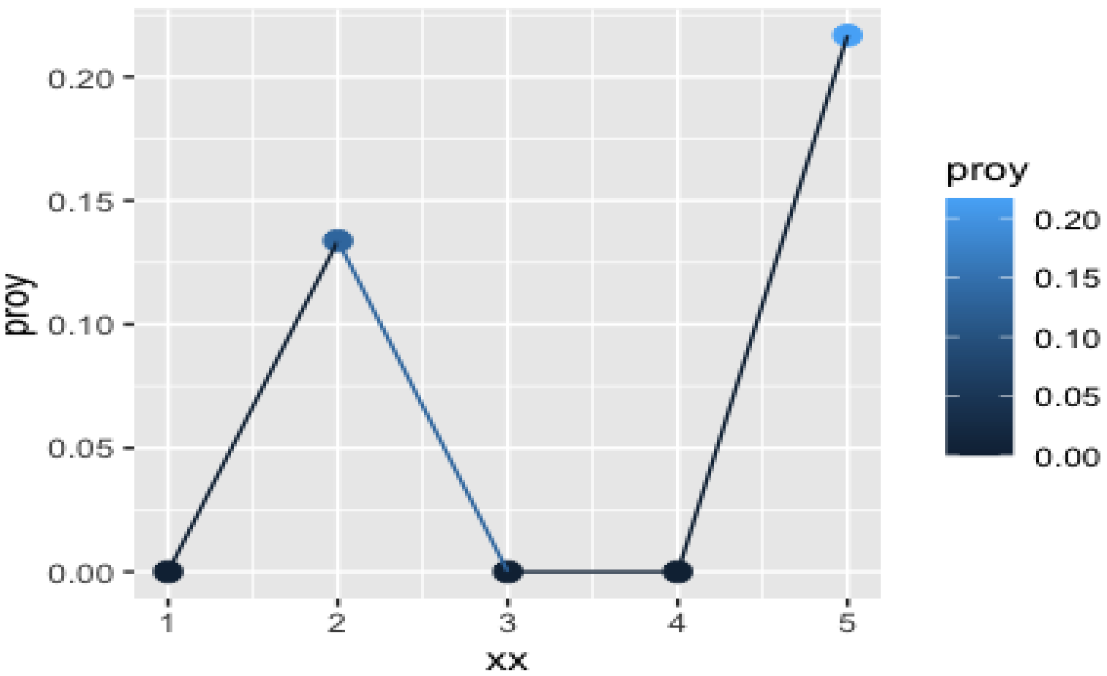
(5)

As we are using the universe $U=\{u_1,u_2,u_3,u_4,u_5,u_6\},$ as a reference system, we have to also compute how the trends considered are projected on the items of $U,$ that is, we have to calculate the coefficients

$${p\left(Trendi\right)|}_{u_j}=\frac{“\mathrm{words}\mathrm{defining}\mathrm{a}\mathrm{fixed}\mathrm{element}{u}_j\mathrm{of}U”\mathrm{AND}“\mathrm{words}\mathrm{defining}Trendi”}{“\mathrm{words}\mathrm{defining}Trendi”},$$

$i=1,2,3,j=1,\dots ,6.$ The results are given in

Table 3. Elements of the Universe vs Trends.

	${\mathit{u}}_1$	${\mathit{u}}_2$	${\mathit{u}}_3$	${\mathit{u}}_4$	${\mathit{u}}_5$	${\mathit{u}}_6$
Trend 1	1	0.1	0.012895	0.726974	0	0.000615
Trend 2	0.560302	0.257538	0.000126	0.071734	0	0.000126
Trend 3	1	0.060742	0.035294	1	0	0.004118

, and their representations can be seen in Figure 3.

So, the (normalized) representations of these three trends on the universe U are

$$P_U\left(Trend1\right)=(0.806174,0.080617,0.010396,0.586068,0.000000,0.000496),$$

$$P_U\left(Trend2\right)=(0.902528,0.414839,0.000203,0.115548,0.000000,0.000203),$$

and

$$P_U\left(Trend3\right)=(0.706233,0.042898,0.024926,0.706233,0.000000,0.002908).$$

(6)

In the next step, we compute the projections of A on the three trends. The representation of A on the universe $U,$ taking into account the values presented in Table 1 and making the convex combination with coefficients $w_1=0.4,$$w_2=0.2$ and $w_3=0.4,$ is

$$P_U\left(A\right)=(0.939903,0.071555,0.113830,0.145120,0,0.001318),$$

where the ith-coordinate corresponds to the item $u_i,$$i=1,\dots ,6.$ Then, using this expression and the formula proposed for the projection of A on each trend, we get

$${p\left(A\right)|}_{Trend1}:=〈P_U\left(A\right),P_U\left(Trend1\right)〉=0.849728,$$

$${p\left(A\right)|}_{Trend2}:=〈P_U\left(A\right),P_U\left(Trend2\right)〉=0.894764,$$

$${p\left(A\right)|}_{Trend3}:=〈P_U\left(A\right),P_U\left(Trend3\right)〉=0.772190.$$

(7)

Now, we make a change in the Euclidean space of reference. Since we assume that Trend 1, Trend 2 and Trend 3 are the independent components of the system, and taking into account that they are linearly independent, we can define the metric as the distance from the vector represented as the projections of A on each trend to each of these trends, which are considered to be the vectors Trend 1 $=(1,0,0),$ Trend 2 $=(0,1,0)$ and Trend 3 $=(0,0,1).$ That is, if $x=(x_1,x_2,x_3)$ and $y=(y_1,y_2,y_3)$ are generic vectors represented by their coordinates with respect to the basis $\mathcal{T}=\{Trend1,Trend2,Trend3\},$ we define the distance by

$$d(x,y)={\left({(x_1-y_1)}^2+{(x_2-y_2)}^2+{(x_3-y_3)}^2\right)}^{1/2}.$$

After normalization with respect to this distance, we get the desired representation of A over $\mathcal{T},$

$${p\left(A\right)|}_{\mathcal{T}}=(0.583745,0.614684,0.530477).$$

Remark 1.

The proposed change of the Euclidean space is not mandatory. An alternate method can also be used, which would provide slightly different results. Since we have all the vectors already represented in the $6—$dimensional space provided by the use of the universe $U,$ we can use this representation and the Euclidean norm in this space to estimate the Lipschitz extension that is explained in Step (8). In this case, we consider a metric space of 3 vectors—the three trends represented as vectors of ${\mathbb{R}}^6$—, and the vector of 6 coordinates that represents $A.$ We measure the distances among them as the Euclidean norm ${\parallel ·\parallel }_2$ of the difference of the corresponding 6-coordinates vectors.

(8)

Now we compute the Lipschitz extension of the Trend Index $=TI.$ A direct computation using the distances among the three trends given by the metric matrix

$$d=\left[\begin{array}{ccc}0& \sqrt{2}& \sqrt{2}\\ \sqrt{2}& 0& \sqrt{2}\\ \sqrt{2}& \sqrt{2}& 0\end{array}\right],$$

gives the Lipschitz constant of the Trend Index, $Lip$ = 210,712,192. The values of the Trend Index for the three trends are

$$TI\left(Trend1\right)=298.000.000,TI\left(Trend2\right)=7.960,TI\left(Trend3\right)=7.820.000.$$

The distances from A to each of the trends are

$$d(A,Trend1)=0.912420,d(A,Trend2)=0.877857,d(A,Trend3)=0.969043.$$

Thus, we can estimate the Trend Index for the innovation idea A using the mean of the McShane and Whitney extension, obtaining

$$T{I}^M\left(A\right)=105,741,949,T{I}^W\left(A\right)=184,983,129.$$

Thus, taking as extension the mean of these values (interpolation for $\alpha =1/2$), we get the final result

$$TrendIndex\left(A\right)=TI\left(A\right)=145,362,539.$$

If we normalize to the maximum value of $TI$ for all the trends, ($max=298,000,000,$) we get (approximately) the value $0.4878,$ that is, the “Relative Trend Index” is

$$48.78\%\mathit{trend\; of\; the\; innovative\; idea\; A}$$

in relation to the trends set in the model.

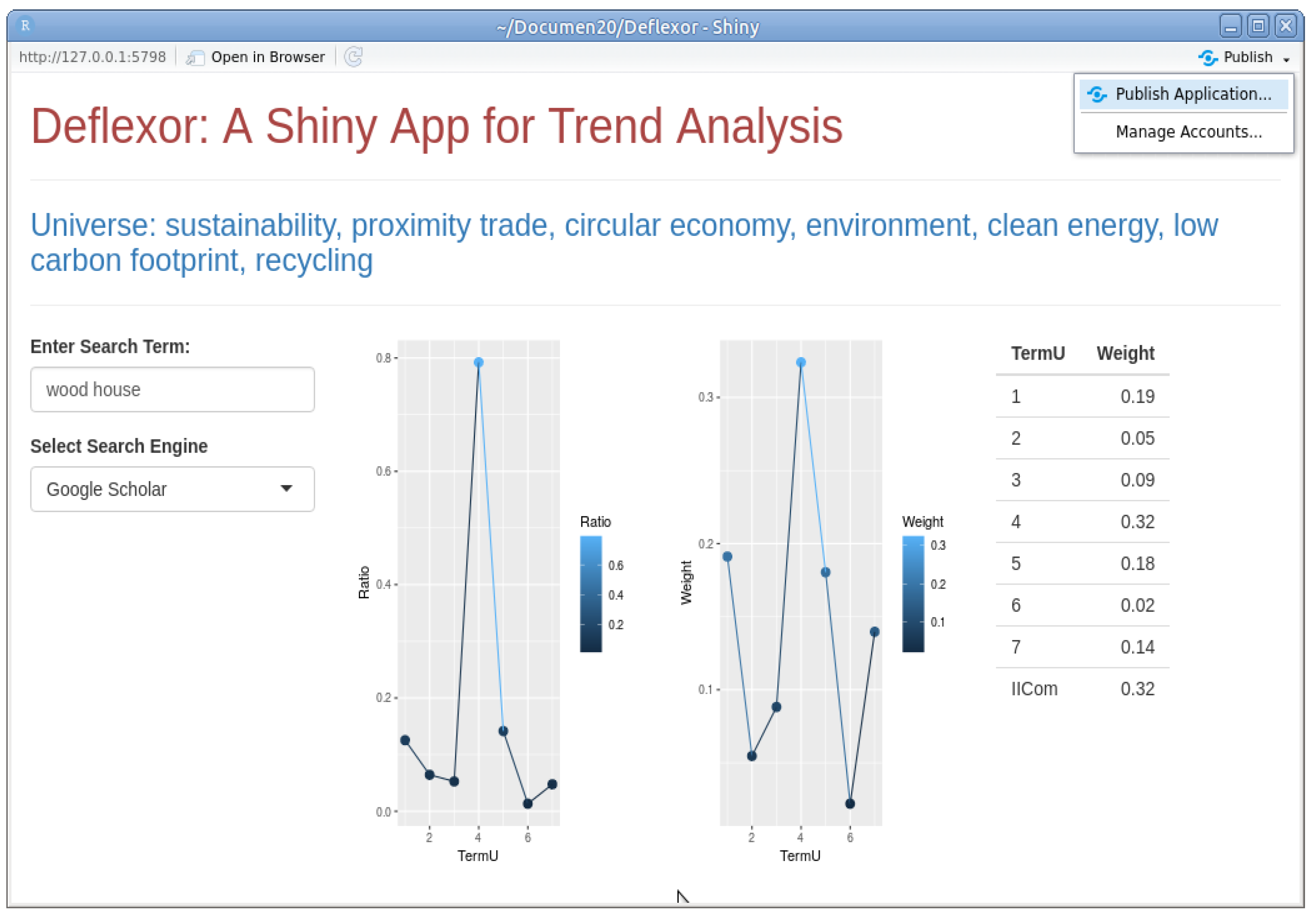
5.3. A Shiny App for Trend Analysis Based on Deflexor

Using this procedure, we built a multi-source platform based on the terminology provided by Deflexor. For each analysis, it is necessary to define a restricted universe, on which the term to be studied is projected. Thus, it is necessary to first fix a specific aspect of the trends that can be studied using the Deflexor conceptual map. That aspect defines the universe in each case.

Figure 4 shows a simulation of how the device works. The selected universe is presented at the top of the page. Just below, on the left side, you can type the term you want to project and also the search engine you want to use: we chose Google Scholar in this case, but several options are offered. The calculations to obtain the individual projections were done as explained earlier in this section, but using Google Scholar instead of Google Search. Therefore, it provides information about the link between the search term and each of the elements of the universe when the search is focused on academic journals and general academic material. The graph on the left shows the values of the projection on each term of the universe (indexed by the order number), and the one on the right gives the relative weight of each of them. The table shows the numerical values of these weights. The last value (IICom) corresponds to the aggregate index that provides the overall value of the projection of the item “wood house” on the universe. Both the individual projections and the relative weights are used to obtain the convex combination that gives the index IICom.

6. An Advanced Example

In this section, we explain how the proposed tool can be applied to help in a given trend analysis. In this case, we use the Google Trends App. By means of this tool it is possible to download massive data on the (relative) number of searches for terms on the Internet, and this is the starting point of our analysis. As a general question, we are interested in the analysis of how some general issues related to the protection of the natural world can influence the acceptance of a certain furniture design.

6.1. The General Setting

Let us follow the outline provided in Section 4.2 and Section 4.3. We start by defining a universe of words extracted from the Deflexor model related to innovation and the environment, associated with general keywords that users identify with environmental care (such as “sustainable”), natural materials (such as “wood”) and also negative words (such as “waste”) that may appear in the search as opposing terms. We include the word “furniture” to also give a reference term in the field, which allows us to relate the search to the class we are interested in analyzing. For simplicity, we set for this example the following small set of words

$$U=\left\{“\mathrm{sustainable}”,“\mathrm{environment}”,“\mathrm{wood}”,“\mathrm{waste}”,“\mathrm{furniture}”\right\}.$$

The size of the universe for a trend analysis will depend on the problem; as a general reference, a set from 5 to 30 words is expected. It is assumed that this set is chosen on the advice of experts; of course, the help of other analytical tools to determine the best set of n terms would improve the results. The data provided by the Google Trends App, which we used over a time interval of three months, gives the vector of the relative number of occurrences of the word per day over the whole period. We used the R package “gtrendsR” for the calculations. Note that Google Trends does not give the actual value of searches per day, but the comparison between the occurrence of a list of terms, giving to the maximum of all of them the value 1. Therefore, each word B in U is represented by a vector of $3\times 30$-coordinates containing the relative appearance in searches per day of the word (each day at each coordinate) and are normalized by the maximum value of all coordinates, to which the value 1 is given. Thus, any term A that we want to investigate is represented in our algorithm by a vector of 90-coordinates; we identify the word A with its corresponding vector.

Once we have accepted the universe of words, we will need to define a trend success index for the five words in U, which will provide the general reference for the evaluation of the success of any other term. The first step is to consider a projection $P_B\left(A\right)$ defined for each $B\in U$ for every term $A.$ In this case, we use the formula

$$P_B\left(A\right):=max{\left(1-\frac{\alpha (A,B)}{\pi /4},0\right)}^{1/2}·{\left(1-\frac{{\parallel A-B\parallel }_1}{max(\parallel A{\parallel }_1,\parallel B{\parallel }_1)}\right)}^{1/2}$$

where $\alpha (A,B)$ is the so called geodesic distance—the angle defined by the words/vectors A and B—that is

$$\alpha (A,B)=arccos\left(\frac{\langle A,B\rangle }{{\parallel A\parallel }_2·{\parallel B\parallel }_2}\right).$$

The meaning and relevance of this projection is deeply related to the nature of the problem. As we have said, the vector giving the number of searches per day is extracted from Google Trends. This tool uses Big Data techniques to manage the information of all searches performed by all Google Search users worldwide. The vectors obtained provide not only information on the comparative number of searches for the different terms, but also the extent to which these searches are correlated (i.e., the extent to which the search for a given word is proportional to the search for another word every day). Note that the first factor in the formula tends to equal one when the pattern of searches for A and B is similar, but (eventually) of a different scale: B might have 100 times as many searches as A, but this factor will equal one if they follow the same pattern. Indeed, $alpha$ gives information similar to that provided by the well-known cosine similarity. We divide $\alpha$ by $\pi /4$ to include a security criterion, making the projection equal to 0 in case the pattern of A and B are so different that no correlation can be accepted. The second factor measures the proximity in norm of A and $B,$ giving information about the comparison of their sizes, and is equal to one if the vectors coincide. Both aspects are fundamental to define the projection of one word onto the other, as we want to know if they are equally relevant in the volume of user searches, but also if they have the same trend pattern. Note that the meaning of this projection is not the same as that of the metric used in the Section 5. Each projection provides a different type of analysis, which means that our technique can generate many complementary tools.

We define the projection vector $P_U\left(A\right)$ as the 5-coordinates vector of the projections on each term of U, that is

$$P_U\left(A\right):=\left(P_{B_1}\left(A\right),P_{B_2}\left(A\right),P_{B_3}\left(A\right),P_{B_4}\left(A\right),P_{B_5}\left(A\right)\right),$$

where

$$\{B_1,B_2,B_3,B_4,B_5\}=\left\{“\mathrm{sustainable}”,“\mathrm{environment}”,“\mathrm{wood}”,“\mathrm{waste}”,“\mathrm{furniture}”\right\}.$$

Another element needed to construct the index extension method for all terms of D is the metric q. We take the distance q in the set D of all possible projections of terms onto the universe U as the Euclidean norm,

$$q(A,B)=\parallel P_U\left(A\right)-P_U{\left(B\right)\parallel }_2,A\in D,B\in U.$$

The Euclidean norms of the vectors associated with all the terms in U allow us to compare their sizes. This information can be used to estimate the relevance of the words in U; after normalization, we obtain the corresponding relative weights.

$$W=(0.06678745,0.11303280,0.56267951,0.09079195,0.16670828).$$

As the norm gives a direct measure of the term’s appearance in Google searches, it represents the importance of each word in U for the trend analysis. This will be used for the definition of the final index. Let us follow the steps of our proposed procedure.

(1)

We fix the proposed “idea” with a set of terms as simple as possible. An example would be $A=\left\{“\mathrm{plastic}”,“\mathrm{chair}”\right\}$ in case we want to analyze the trends about the acceptance of a plastic chair with respect to the trends of the universe $U.$

(2)

We compute the projection $P_U\left(A\right),$ that gives for the term “plastic”

$$P_U\left(A_1\right)=(0.2205327,0.2407994,0.4085899,0.3055694,0.4510627),$$

(Figure 5a), and for the word “chair”

$$P_U\left(A_2\right)=(0.1722883,0.2825582,0.2441297,0.2628509,0.4357773),$$

(Figure 5b).

(3)

We measure the (quasi-)distance $q(A,B)$ from $P_U\left(A\right)$ and any fuzzy subset B that represents a trend.

(4)

$q(A,B)$ represents a measure of how close is our original idea to the trend $B.$ Computing the distances with respect to any trend, we can measure “how far our idea is” from this trend.

6.2. How to Choose the Best Design Project According to Our Trend Analysis

Let us define now the index that could be applied to measure the success of a certain type of furniture with respect to the trends that are represented by the universe $U.$ Using it and the extension algorithm for the index explained in Section 4.3 we complete the picture of our analytic tool. After an analysis of a list of different classes of furniture extracted from the list given in [44], our group of experts decides that the following index $I_F$ gives a reasonable measure of the fitting of the elements of the subset

$$D_0:=\left\{“\mathrm{chair}”,“\mathrm{table}”,“\mathrm{mirror}”,“\mathrm{bed}”,“\mathrm{sofa}”\right\}$$

with the current trends in furniture design in the universe U. Indeed, the index $I_F$ given by

$$I_F\left(A\right)=〈\left(min\left(\frac{{\parallel A\parallel }_1}{\parallel B_1{\parallel }_1},1\right),\cdots ,min\left(\frac{{\parallel A\parallel }_1}{\parallel B_5{\parallel }_1},1\right)\right),W〉$$

will provide the desired tool. The set $D_0$ is chosen following the advice of the expert by means of the conceptual analysis based on the Deflexor framework. The central idea is that the behavior of these pieces of furniture with regard to Google searches—analyzed using the Google Trends App—provides an overview of current trends in furniture design.

At this point, the analytic system is prepared to be used. The universe that define the main terms in which we want to center our analysis has been defined by an expert selection based on the Deflexor general diagram. The objects that we intend to define as main references for comparing with other furniture items are the ones presented in $D_0.$ We use the McShane–Whitney extension method for Lipschitz regression, which is provided by the formulas

$$Ext\left(C\right)=\frac{1}{2}{I_F}^M\left(C\right)+\frac{1}{2}{I_F}^W\left(C\right)$$

$$=\frac{1}{2}\underset{A\in D_0}{max}\{I_F\left(A\right)-Lip{q}_U(A,C)\}+\frac{1}{2}\underset{A\in D_0}{min}\{I_F\left(A\right)+Lip{q}_U(A,C)\},C\in D.$$

The value of the Lipschitz constant needed to apply our algorithm of Lipschitz regression is $Lip=0.89863.$ The values of the projections of the elements of the set $D_0$ on the universe U can be seen in

Table 4. Projections for the terms considered, together with the corresponding values of the (extended) index $I_F/Ext$.

Terms	Sustain.	Environ.	Wood	Waste	Furniture	${\mathit{I}}_{\mathit{F}}$/Ext
chair	0.1722	0.2825	0.2441	0.2628	0.4357	0.4867
table	0.1562	0.1762	0.4399	0.1623	0.25	0.7421
mirror	0.1645	0.2096	0.4170	0.1805	0.3017	0.7069
bed	0.1807	0.2511	0.3723	0.2779	0.3748	0.5948
sofa	0.0799	0.1069	0.312	0.1004	0.1544	0.7416
desk	0.1317	0.2356	0.1891	0.2417	0.1756	0.632
cabinet	0	0	0.0693	0	0.163	0.721
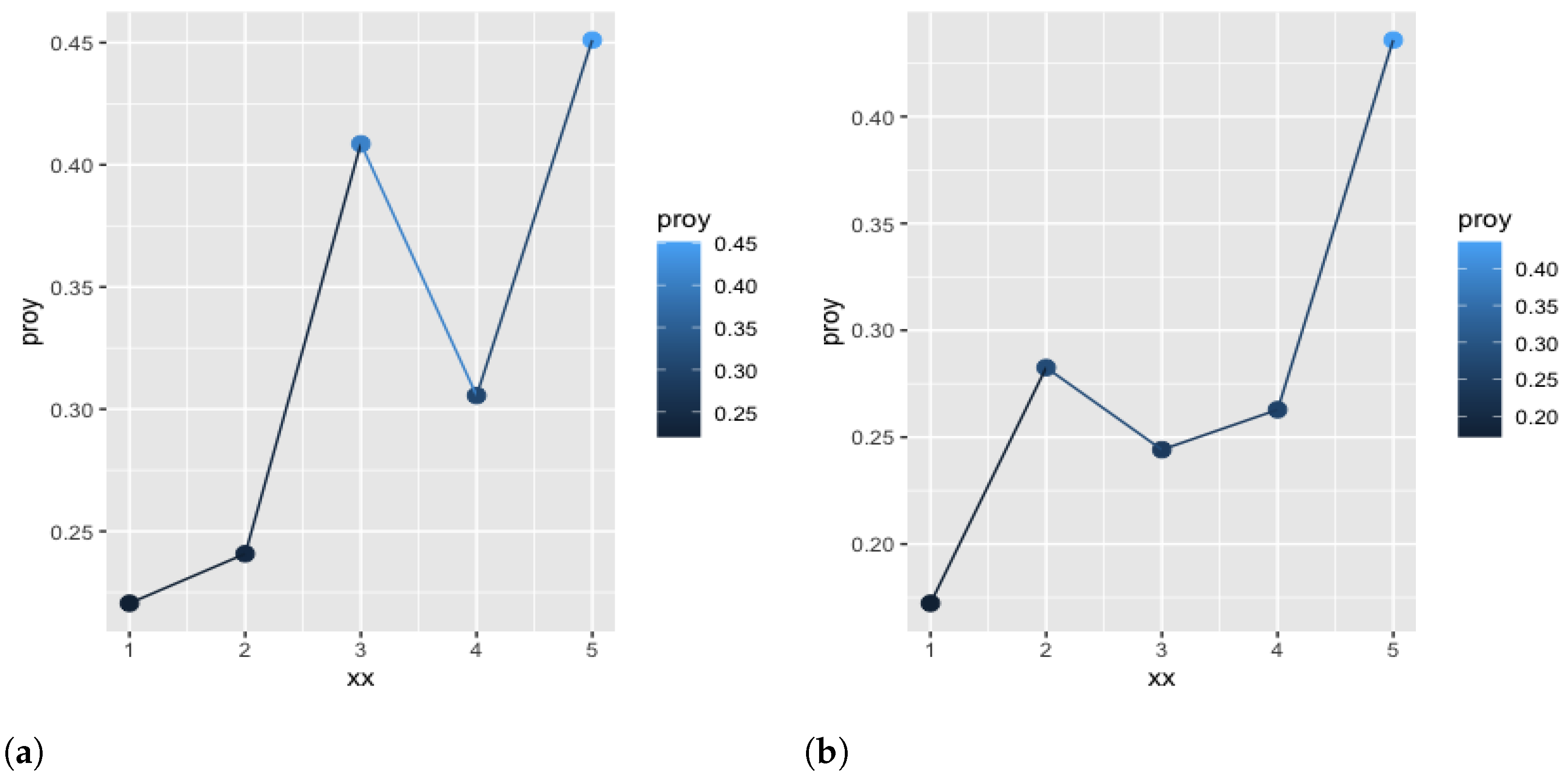
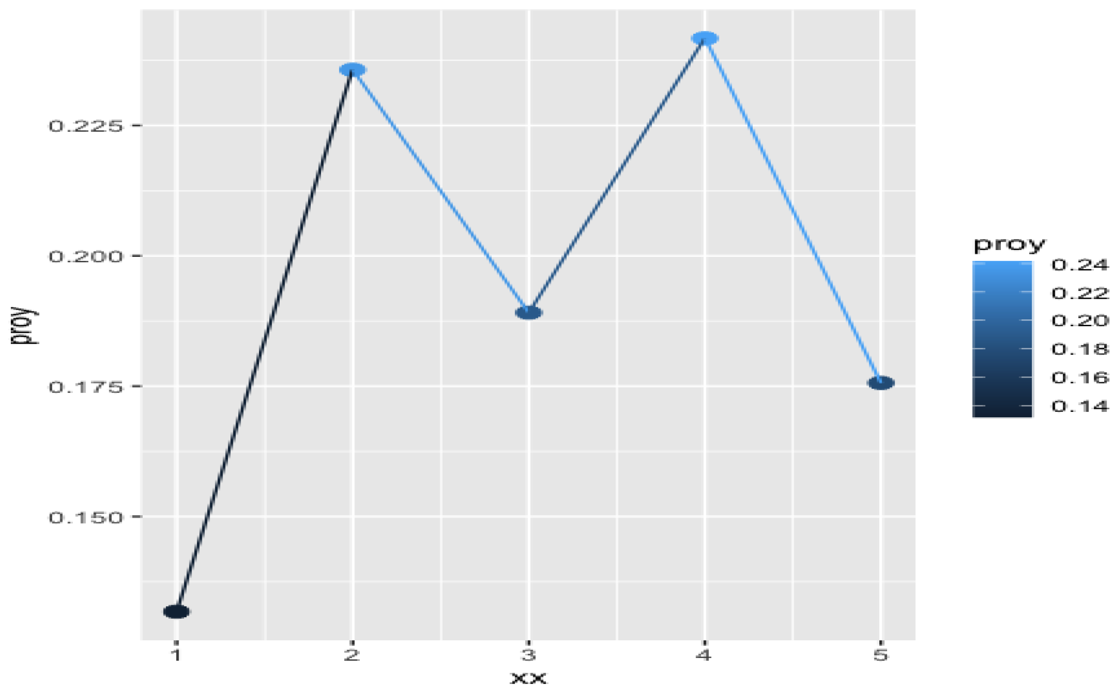
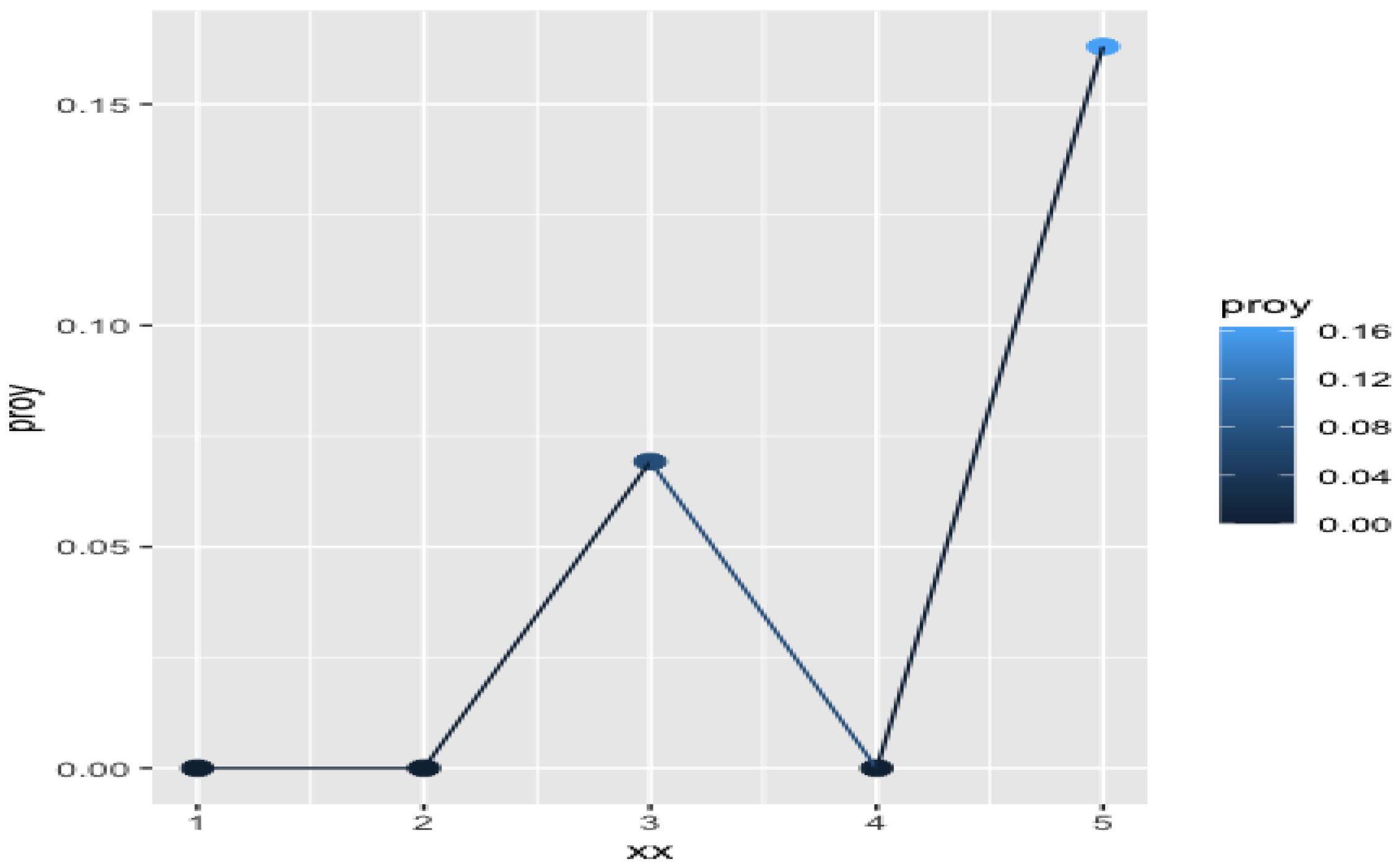
carpet	0	0.1337	0	0	0.2168	0.6743

below. These terms have been checked by the experts, who agree in their central role for following the trends of the furniture market, and the rest of the items have to be referred to this set. To show the result, we present in the final lines of Table 4 and in Figure 6, Figure 7 and Figure 8 the projections $P_U\left(C\right)$ on U of the terms $C=“\mathrm{desk}”,“\mathrm{cabinet}”,“\mathrm{carpet}”$ together with the value of the extended index $Ext$ computed for these items.

It can be seen that the projection values for the term “desk” are better than for the other items, as there are no zeros in their projections and overall the values are higher. However, the values of the index $Ext$ suggest the choice of the other options, “cabinet” and “carpet”—$0.721$ and $0.6743$ versus $0.632$—even though the latter is not properly a piece of furniture like the others. The reason is that, summing up the effect of all the coordinates, the vector representing “cabinet” and “carpet” are more similar to that of “sofa” than in the case of “desk”. As “sofa” has one of the highest values of $I_F,$ this could justify the values of the extended index $Ext$. Therefore, the system proposes “cabinet”—or even “carpet”—as a better choice than “desk” to start with a new design product.

We have shown a simple—but realistic—use of our tool for trend analysis. The reader can see that the expert criteria for the definition of the relevant term sets has to be combined with the use of the tool, and the results largely depend on this preliminary work. The final product is then a versatile platform, which should be used by the analyst as a framework to integrate both data retrieved automatically from the Internet and term/conceptual analysis in a common environment. The result is intended to be a holistic tool for analysis and prospects of design trends. The continuous feeding of data used for the calculation of the indices, as well as the incorporation of new terms already tested, would provide the basis for a continuous updating of the platform. This could take the form of a reinforcement learning system of artificial intelligence, which would selectively incorporate new data based on the observed results, following the time axis.

7. Discussion: Using Deflexor to Motivate Open Innovation

The analytical tool explained in this paper is intended to be a new instrument for Open Innovation engineering [45]. As a result of the collaboration of experts in a given design field and technicians, the model provides an analytical platform to be used in the elaboration of preliminary studies on how new products can enter the market, allowing managers to get an idea of how a new design object can be accepted at a given point in time. Once the general methodology is fixed, it needs to be adjusted to create a specific platform for each field of application. This is the point at which the professionals of a given company have to work together with the designers of the system to adapt the general trend analysis to the specific field of design in which the company is interested. These experts not only have to provide the general ideas about the field, but they have to help to prepare the universe of terms needed for the analysis, and even the relationships between them in order to build—together with the data scientists and linguists—a language structure as developed as possible. The aim is to foster a dynamic point of view in the design world, implementing new technologies for the continuous search for market trends in the context of open innovation. Any new product must be checked in advance by means of the most specialized multi-source information technology, which provides accurate pictures of the current state-of-the-art.

Trend analysis guided by expert teams has to grow together with current developments in software technology. Finding the right context for cooperation could result in the implementation of Open Innovation procedures in design companies, which have to understand that innovation, Big Data and information technology are fundamental for the success of their projects. In certain fields, innovation has traditionally had a relevant internal motivation, as is the case in software engineering. This approach is increasingly complemented by an Open Innovation approach in which external motivation plays an increasingly important role [46,47]. In this key technology field, it is also observed that start-ups and small companies are more inclined to introduce innovation schemes than larger ones, which in a way confirms the idea that small structures allow for faster adaptive changes [48].

In general, open innovation in a given field can be understood as a dynamic process that starts with a social trend, often carried out by entrepreneurs who facilitate new combinations between market and technology. Then, large companies—following market pressure—start to act using various channels, resulting in the mechanism of economic growth. The elements that make up the ecosystem necessary for this process to take place are represented in the so-called quadruple helix model: industry, society, academia—as a necessary source of scientific and technological knowledge—and government, which increasingly plays a facilitating role, rather than the classic regulatory role [48]. Recently, many specific studies have been carried out focusing on some fields where Open Innovation is changing the way things are done [49]. But each specific environment needs special ways of implementing this working philosophy (see for example [50] for innovation in the field of food). In all of them, however, new design strategies have to incorporate both external innovation technology and the expertise of internal professionals.

8. Conclusions

We have developed a methodology to quantify the degree of innovation of projects and ideas according to current trends. The measurement system is based on the prior determination of a certain number of recognized trends in a given field, that have to be structured as a “universe”, that is a set of terms and relations among them. Innovative ideas are understood as general concepts, proposals for action, ways of doing things, widely accepted products or any other semantic element that can be codified by some short linguistic expression, preferably words and relations between words. Our aim was to provide a general method for the automation of trend analysis, which necessarily has to be based on the determination of the framework by the analyst.

To do this, we first set a universe U of words/concepts/notions that are understood to be significant in the given field of analysis. The canonical example of such a universe U is a specialized ontology of a certain technical field. We then introduce our innovative idea and determine the set of trends that we consider to be related to it, in order to contrast both elements through the framework that defines the universe $U.$ We need a method of quantification, and we define it through the notion of projection, which consists of a particular way of calculating the “semantic component” of a term “A” of the term “B” with respect to a predefined projection tool. We have used as an example of such a tool the rate of documents in which “A” appears along with “B”, with respect to the total number of documents in which “B” appears in a Google search. The idea is to aggregate several of these simple projections to obtain a characteristic composite projection that meets the requirements of the users in each particular design environment.

From the mathematical point of view, the model consists of a (quasi-)metric space of fuzzy subsets of $U.$ Several metrics are proposed, using as supporting formalism the representation as vectors of linear spaces, what facilitates the use of norms, although this is not the only option provided. We then introduce a method for measuring the relevance of a trend, and use the theory of Lipschitz functions to extend the obtained values to all the elements of the (quasi-)metric space. This gives an evaluation of the innovative idea, and would allow the use of a reinforcement learning method as the one given in [51,52] for continuously improve the result by introducing at any moment updated information, allowing also the direct action of experts to correct dysfunctional outcomes if needed (supervised learning). An App based on our ideas which uses multi-source projections has been already designed, and has been presented here too.

The last section presents an example of trend analysis using our procedure: a case is presented in which a group of designers has to choose between three furniture-related items in view of their potential market acceptance. A precise explanation of how to do this using our tool is given, together with a description of the mathematical elements used for this purpose.