Kappa Distributions: Statistical Physics and Thermodynamics of Space and Astrophysical Plasmas

Division of Space Science and Engineering, Southwest Research Institute, San Antonio, TX 78238, USA
Universe 2018, 4(12), 144; https://0-doi-org.brum.beds.ac.uk/10.3390/universe4120144
Submission received: 11 October 2018
/
Revised: 4 December 2018
/
Accepted: 5 December 2018
/
Published: 7 December 2018
(This article belongs to the Special Issue Selected Papers from the 7th International Conference on New Frontiers in Physics (ICNFP 2018))
Abstract
:Kappa distributions received impetus as they provide efficient modelling of the observed particle distributions in space and astrophysical plasmas throughout the heliosphere. This paper presents (i) the connection of kappa distributions with statistical mechanics, by maximizing the associated q-entropy under the constraints of the canonical ensemble within the framework of continuous description; (ii) the derivation of q-entropy from first principles that characterize space plasmas, the additivity of energy, and entropy; and (iii) the derivation of the characteristic first order differential equation, whose solution is the kappa distribution function.
1. Introduction
Kappa distributions have become increasingly widespread across the physics of astrophysical plasma processes, describing the velocities and energies of particles from solar wind and planetary magnetospheres to the heliosheath, and beyond to interstellar and intergalactic plasmas (see the book [1,2], and the reviews [3,4,5]).
A breakthrough in the field came with the connection of kappa distributions with statistical mechanics and thermodynamics. Empirical kappa distributions were introduced in the mid-1960s by Binsack (1966) [6], Olbert (1968) [7], and Vasyliũnas (1968) [8]. However, the statistical origin of kappa distributions came from the maximization of Tsallis q-entropy [9], under the constraints of canonical ensemble (e.g., see [2,10,11,12]). Note that the label q stands for the mono-parametrical entropy expressed in terms of q-index, or equivalently, in terms of kappa index, i.e., [2]. On the other hand, the thermodynamic origin of these distributions and their associated entropy (the q-entropy) was also shown from first principles (e.g., see [13,14]); namely, the most generalized form of particle distribution function that can be assigned with a temperature is that of kappa distributions (or a combination thereof). Then, “thermalization” is the characterization of a particle system residing in any stationary state assigned by a temperature; in these states, the particle velocities or energies are stabilized into kappa distributions.
Kappa distributions are consistent with thermodynamics, but this fact alone cannot justify the generation and existence of these distributions. The connection of kappa distributions with statistical mechanics and thermodynamics should not be considered as one of the possible mechanisms of kappa distributions. On the contrary, once a kappa distribution of particle velocity or energy is generated by a certain mechanism, the preservation–or non-preservation–of this distribution for describing the particles of the systems is a matter of thermodynamics alone.
There are various mechanisms capable of generating kappa distributions in space and astrophysical plasmas. Some examples are superstatistics [15,16,17,18], the effect of shock waves [19], weak turbulence [20], turbulence with a diffusion coefficient inversely proportional to velocity [21], the effect of pickup ions [22], pump acceleration mechanism [23], and polytropic behavior [24,25,26]; (see also [1], chapters 5, 6, 8, 10, 15, and 16). Also, common processes characteristic of space plasmas, such as the Debye shielding and magnetic coupling, have an important role in the generation of kappa distributions in plasmas [27].
In general, long-range interactions or other causes of local particle correlations implicate the particle system in the statistical framework of kappa distributions [14,27,28]. Such an example is the state of a charged test particle in a constant temperature heat bath of a second species of charged particles, modeled by Shizgal (2018) [29]. The time dependence of the distribution function of the test particle is given by a Fokker–Planck equation for Coulomb collisions and wave–particle interactions; the stationary state of this equation can be described by kappa distributions (for certain choices of the involved parameters). In particular, the model leads to an ordinary first order differential equation, characterizing the stationary state of the Fokker–Planck equation; the solution of this differential equation is a kappa distribution.
In this paper, we show recent developments on the theory of kappa distribution, with emphasis on the differential equations leading to kappa distributions; we also show that the differential equation taken from the Fokker–Planck equation model of Shizgal (2018) [29], and from the earlier first principles analysis of Livadiotis (2018) [30], are equivalent. In Section 2, we briefly present the general theory of kappa distributions, and then show their connection to statistical mechanics; for the first time, this is shown within the framework of continuous description and using the kappa index formalism. In Section 3, we present the statistical origin of these distributions and their associated q-entropy from first principles—that is, considering the property of additivity for both the energy and entropy. In Section 4, we show the equivalency of the two characteristic differential equations leading to kappa distributions. In Section 5, we discuss the applications and physical properties of as well as insights into kappa distributions, and several misinterpretations concerning the formalism of kappa distributions. Finally, in Section 6, we summarize the conclusions.
2. Statistical Derivation of Kappa Distributions
Space plasmas are particle systems characterized by local correlations and strong collective behavior among their particles, which can cause significant deviations from the classical framework of Boltzmann–Gibbs (BG) statistical mechanics and thermodynamics. Kappa distributions describe the particle velocities when correlations exist among particles—that is, a typical situation for collisionless particle systems, such as space plasmas. The correlations among particles could be eliminated if particle collisions occurred at a considerable frequency—that is, if the collision frequency ωpl was larger than, or at least comparable to, the plasma frequency νcol. In general, the ratio of those frequencies is of the order of νcol/ωpl~1/ND, where ND stands for the number of particles in a Debye sphere. Also, the ratio of the Debye length λD over the mean free path Lmfp is of the same order, λD/Lmfp~1/ND. Collisional plasmas have large values of these ratios, indicating that correlations among particles can be ignored in such a case; on the contrary, collisionless plasmas have small values of these ratios, indicating important correlations among particles. For space plasmas, ND is up to a billion or even a trillion, indicating highly collisional plasmas, for which collisions cannot eliminate correlations. (For more details, see: [31], Chapter 2; [1], Chapter 5; [32,33]
The physical meaning of the kappa index can be understood through particle correlations. In fact, a simple relation exists between the (Pearson) correlation coefficient R and the kappa index κ—that is, (for particles with d = 3 degrees of freedom) ([28,34]; [1], Chapter 5). The largest value of kappa, , corresponds to the system residing at the classical thermal equilibrium, characterized by the absence of any correlations; the smallest possible kappa value, , corresponds to the furthest state from classical thermal equilibrium, a state called anti-equilibrium [4], which is characterized by the highest correlations.
The connection of kappa distributions with statistical mechanics is through the maximization of q-entropy under the constraints of canonical ensemble—that is, the normalization of the deduced probability distribution to the unity, and the fixed value of the mean kinetic energy to the internal energy per particle, .
The entropy and the constraints are functionals of the velocity distribution.
- -
- Entropy:
- -
- Constraint of normalization:
- -
- Constraint of fixed internal energy per particle:where stands for the smallest speed scale parameter characteristic of the system, hence:defines the number of microstates in the f–D velocity space. The probability distribution scales as ; thus, is dimensionless. We use the particle kinetic energy and mean kinetic energy , which interprets the internal energy per particle.
The q-entropy is interwoven with the escort probability distributions [35], while these two concepts together form the modern non-extensive statistical mechanics [5,36]. The escort probability distribution is constructed from the ordinary probability distribution , through the duality
(The above are still written in the continuous description. For the discrete description, see, e.g., [2]; [1], Chapter 1.)
Within the framework of non-extensive statistical mechanics, the interpretation of the internal energy is given via the escort expectation value of energy, which is
Given the two constraints of Equations (2) and (3), the entropy from Equation (1) is maximized using the Lagrange method—in other words, by using the two Lagrange multipliers λ1 and λ2 to maximize the functional . Therefore, we have
or
because . Hence, we may write
where
In order for the integral in Equation (10) to be zero for every distribution , it is necessary for , hence
The corresponding escort distribution becomes
This is written as
that is, the standard formulation of kappa distribution, where we use (i) the normalization (partition function), given by
and (ii) the notion of temperature, whose inverse is taken from
(More details on the concept of temperature for systems described by kappa distributions can be found in [5]; [1], Chapter 1; [14].)
The dyadic formalism of ordinary/escort distributions is of fundamental importance in modern non-extensive statistical mechanics (e.g., [35,36]; [1], Chapter 1). However, the maximization of entropy can follow an alternative path, in which there is no use for the formalism of escort distributions. In particular, it was shown that this dyadic formalism of distributions can be avoided in order to simplify the theory, but it leads to a dyadic formulation of entropy [30]. According to this, the constraint of internal energy is written as
The entropy maximization in Equation (10) gives the argument I:
thus,
where we substituted
We again substitute the Lagrange multipliers λ1 and λ2 with thenormalization constant or partition function Z and the temperature T, respectively:
Then, after the transformation :
the distribution takes the standard form, as in Equation (14),
We note that we avoid the concept of escort distribution but the kappa index transformation, in Equation (22), leads to a duality of entropy, as shown in [30]—that is, . It is also important to mention that this alternative method of maximization has the advantage that it can be used for any entropic formulae, e.g., in theoretical analyses that seek to retrieve the entropic form considering other first physical principles (Section 3).
3. Statistical Origin of Kappa Distributions
The entropy maximization shown in the previous section cannot be conceived as the statistical origin of kappa distributions. Entropy and distribution are two functions that can be equivalently derived from each other. Given an entropic function, that function can be maximized to find the canonical distribution; also, in reverse steps, given a distribution, we can always find an appropriate functional form of entropy that can be maximized and lead to this desired distribution. Therefore, we need to derive the origin of the kappa distribution, or equivalently, its associated entropy, the Tsallis q-entropy. In particular, we search for the function f(x) that involves in the entropic and distribution functions.
Here we set a discrete energy distribution: energy ε1 with probability p1, energy ε2 with probability p2, …, and energy εw with probability pw. The entropy and its maximization can be generally formulated as follows:
(setting kB = 1). For example, in non-extensive statistical mechanics [37], the entropic function f is mono-parametrical, expressed by the kappa index as shown in Equation (1):
which, for corresponding to BG entropy, is reduced to
Therefore, the statistical origin of kappa distributions coincides with the statistical origin of their associated entropy. Moreover, it has been shown that first principles, such as the additivity of energy and entropy, are sufficient for indicating the specific formula of q-entropy [14].
The probability distributions of , , and , are related to their energies:
where we consider two subsystems, A and B, with respective energy spectra and , associated with the discrete probability distributions and . The total system A + B has energy spectrum , associated with the joint probability distribution . Thus, the additivity of energies, , gives
Applying in both sides of Equation (29), we obtain
This is compared with the additivity of entropy:
We observe that the two functions and have the same additivity property. Therefore, one function f that satisfies the additivity of entropy is the one that obeys the proportionality, , or the differential equation
Setting and (that is, setting the entropic unit kB equal to 1), we end up with
The solution of this differential equation is the entropy associated with kappa distributions, or the q-entropy.
4. Characteristic Differential Equation
The derived differential Equation (33) in the previous section has as a solution the entropic function f(x) of in Equation (24). Here, we derive the characteristic differential equation of the kappa distribution function, p(ε).
Equation (28) is written as
and in combination with Equation (33):
we have
We differentiate
Hence
Substituting , we obtain
The second Lagrange multiplier λ2 is related with the inverse temperature , thus
where we used Equation (16) and the equality
Also, the first Lagrange multiplier, λ1, can be set to 1 (see more details in [30]), hence
Then, the transformation of kappa in Equation (22) brings us finally to the differential equation
or, expressed in terms of speeds:
This coincides with the differential equation derived from the model of Shizgal [29]. The time dependence of the distribution function of the test particle is given by a Fokker–Planck equation for Coulomb collisions.
5. Discussion: Applications and Physical Insights
The kappa distributions have a tremendous number of applications in space and astrophysical plasmas, such as the inner heliosphere, including solar wind (e.g., [13,20,26,38,39,40,41,42,43,44,45,46,47,48]), solar spectra (e.g., [49,50]), the solar corona (e.g., [51,52,53,54]), solar energetic particles (e.g., [55,56]), corotating interaction regions (e.g., [57]), and related solar flares (e.g., [21,33,58,59]); planetary magnetospheres, including the magnetosheath (e.g., [60,61]), magnetopause (e.g., [62]), magnetotail (e.g., [63]), ring current (e.g., [64]), plasma sheet (e.g., [65,66,67]), magnetospheric substorms (e.g., [68]), Aurora (e.g., [69]); magnetospheres of giant planets like the Jovian (e.g., [70,71,72]), Saturnian (e.g., [73,74,75,76]), Uranian (e.g., [77]), and Neptunian (e.g., [78]); magnetospheres of planetary moons, such as Io (e.g., [79]) and Enceladus (e.g., [80]); cometary magnetospheres (e.g., [81,82]); the outer heliosphere and the inner heliosheath (e.g., [13,22,83,84,85,86,87,88,89,90,91,92,93,94,95,96,97]); beyond the heliosphere, including HII regions (e.g., [98]), planetary nebula (e.g., [99,100]), and supernova magnetospheres (e.g., [101]), and in cosmological scales (e.g., [102]). The kappa distributions have also been applied in general to plasma-related analyses (e.g., [11,92,103,104,105,106,107,108,109,110,111,112,113,114,115,116,117,118,119,120].
The plethora of these applications stands on the fact that the kappa distributions are the most general formulations of particle velocity distributions that can be assigned with a temperature [13]. On the other hand, the kappa index that labels and governs these distributions constitutes a new thermodynamic variable, equally important as the temperature.
The kappa index depends on the dimensionality of the problem—that is
where the involved “constant” means that the difference is invariant under changes of the dimensionality, e.g., the degrees of freedom or the dimensionality of the kappa distribution we choose to use in our analyses. This invariant quantity has the meaning of the actual kappa index, namely, it indicates the stationary state in which the system resides; it is noted by κ0, as of zero dimensionality kappa ([27,33]; [1], chapters 1 & 3).
In terms of the invariant kappa index, the kappa distribution is written as:
The corresponding kappa distribution of the kinetic energy, , is
In terms of the standard kappa index, , the distributions become:
and
Note that the notion of kinetic energy is given by the subscript K (capital letter in non-italics).
The invariant kappa index, κ0, is of fundamental importance in the theory and applications of kappa distributions. The kappa distribution describes all the correlated particles together. For N correlated particles, with d degrees of freedom per particle, the total degrees of freedom becomes f = N·d, hence
while the distribution of the energy per particle is
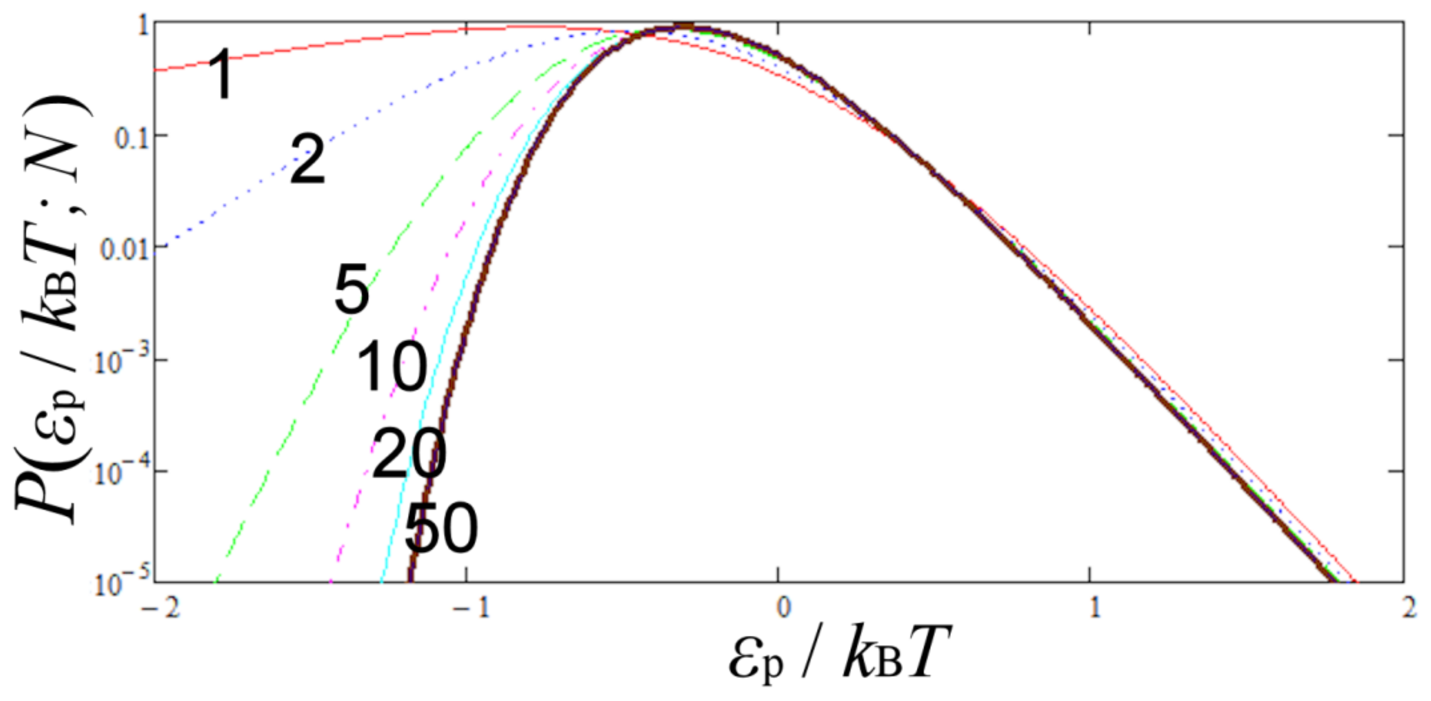
In the thermodynamic limit, , Equation (50) becomes
Note that this distribution can be expressed in terms of the inverse Gamma function [27]. Figure 1 plots the kappa distribution of the energy per particle from Equation (50), expressed in terms of , and for various numbers of correlated particles N, from N = 1 to N = 50, practically tending to infinity, as shown in Equation (35).
Therefore, the stationary state that characterizes the particle system can be described, in general, by three parameters: the temperature T and kappa κ0, which constitute the two independent intensive thermodynamic quantities, and the number of correlated particles N. The same three parameters characterize the corresponding entropy that describes the given particle system. The entropy associated with kappa distributions has been developed in [93], [1] (Chapter 2), and [14]. It constitutes the generalized Sackur–Tetrode entropic formula, given by
or
where we used the deformed exponential and logarithm functions, i.e., and (e.g., see: [1], Chapter 1). The parameter T0 constitutes the minimum possible temperature for the entropy to be positive: , where C = (9π/2)1/3/e ≈ 0.89. The length parameter is interpreted by the interparticle distance b~n-1/d for collisional particle systems, or by the smallest correlation length, such as, the Debye length λD for collisionless particle systems. The parameter gκ is a function of the kappa index κ0 and the number of correlated particles N; a large N becomes gκ ≈ 1. The phase-space cell parameter is interpreted by the Planck’s constant for collisional particle systems, or by the large-scale quantization constant for collisionless particle systems (e.g., [1], Chapters 2 & 5; [14,27,33,121,122,123,124]).
Equation (53) can be written as ; differentiating it in terms of T, and using the equipartition theorem for the internal energy [2], we derive
which constitutes the thermodynamic definition of temperature, generalizing the classical case of
Indeed, as shown by [14,125], all the particle systems that are in thermal equilibrium to each other have the same value of the quantity given by the functional of entropy S and internal energy at the left-hand side of Equation (54). This quantity can be written as
where the auxiliary notion of entropy is connected with the actual entropy S through [30]. However, the temperature is not the only intensive thermodynamic parameter characterizing particle systems. Another thermodynamic parameter is the notion of kappa, whose thermodynamic definition is given as follows.
When the thermal equilibrium of a particle system is disturbed by adding a small entropy dσ into it, the final entropic deviation, after the thermal equilibrium is restored, is dS, according to
which constitutes the generalized thermodynamic definition of kappa. Again, as it was shown by [14], all the particle systems that are in thermal equilibrium to each other have the same value of the quantity given by the functional of entropy S and internal energy at the left-hand side of Equation (57).
According to [14], the zeroth law of thermodynamics indicates that temperature and kappa are the two independent parameters spanning the two-dimensional (2-D) abstract space of thermodynamics. Therefore, temperature is not the only intensive thermodynamic parameter, but both the temperature and kappa are needed for characterizing thermal equilibrium; the former shows the way entropy varies with internal energy, e.g., when heat is exchanged among two systems, while the latter shows the way that entropy partitions. Then, particle systems in contact, capable to exchange heat and entropy, are eventually stabilized into stationary states, which are not described only by a Maxwell–Boltzmann distribution, but generally by a kappa distribution function.
Before these developments, it was thought that the only intensive thermodynamic parameter characterizing particle systems at thermal equilibrium is temperature, and this is the only parameter that should be included in the classical statistical mechanics and kinetic theory of gases. For this reason, misinterpretations may occur when attempting to understand the thermodynamics of non-extensive statistical mechanics using classical definitions that do not apply in the general case, such as Equation (55) (e.g., [126]).
Such a misinterpretation concerns the meaning and determination of temperature. In particular, instead of the actual thermal speed θ, a kappa-dependent thermal speed may be used, defined by (e.g., see [127,128]). Then, the distribution in Equation (47) becomes
The rationale of Equation (58) is that Θ coincides with the most frequent speed in the co-moving frame (), though this interpretation fails for d = 1. As it was stated in [1]: “Why should utilize the most frequent speed u and not the most frequent square root of speed , or even some other power uα or general function g(u)? If we argue that these functions may lack of physical meaning, then how about returning to the kinetic energy, whose mean value defines the temperature in accordance with thermodynamics”.
Temperature is a thermodynamic variable independent of the kappa index, and it is invariant under the system’s transitions to different kappa indices. The same system will have the same internal energy or temperature for any kappa index, even when the latter is infinity and the distribution becomes Maxwellian. However, if Θ was a thermal parameter independent of the kappa index, then the internal energy would have included the kappa index. As it was stated in [106], “clearly, from the definition of temperature, all distributions with the same mean energy per particle have the same temperature”. Therefore, care must be shown, since this distribution cannot be investigated in terms of Θ, as it would have been if this was an independent parameter; the actual thermal speed θ must be used instead. (For more misinterpretations and their resolution, see: [1], Chapter 1.8.3.)
Furthermore, we mention that the notions of temperature and kappa that characterize the generalize description of thermodynamics are the same for anisotropic kappa distribution of velocities/energies (e.g., [129]). Such anisotropies occur when the particle kinetic energy is stabilized in non-equal portions among particle kinetic degrees of freedom. Therefore, the equipartition theorem cannot be applied to each of the three degrees, but to all of them together; thus, the temperature is still given by the mean of the total kinetic energy. The main and most frequently used formulations of anisotropic kappa distributions are those describing plasma in the presence of an ambient magnetic field. In this case, there is anisotropy between the velocity components (parallel, , and perpendicular, ) to the field. We have two main cases (e.g., [1], Chapter 4; [5]):
(1) when the parallel and perpendicular degrees of freedom are correlated to each other:
(2) when the parallel and perpendicular degrees of freedom are independent to each other:
where we set and . For all the above, the temperature and thermal speed are given by
The reader can find the more complicated cases of moderate correlation among the degrees of freedom in [1].
In addition, we have to mention the importance of the power-law behavior of kappa distributions at high energy regions. Indeed, kappa distributions have received impetus, as their Maxwellian “core” and power-law “tail” features provide efficient modelling for observed distributions throughout the heliosphere. Both the Maxwellian core and power-law tail can support useful techniques for finding the values of temperature and kappa. Some examples are the methods of exploiting the Maxwellian behavior of kappa distributions at the core [26,27,117] and the power-law behavior of kappa distributions at the tail [88,89,90]. Nevertheless, care must be shown when using power-laws in general. The basic failures of pure power-laws (or combinations thereof) for describing the velocity/energy distribution functions are the following: (i) normalization—namely, they cannot be normalized; (ii) correspondence, where they do not include the classical limit of Maxwell distribution; and (iii) inconsistency, meaning they are not consistent with zeroth law of thermodynamics. On the other hand, kappa distributions (i) can be normalized; (ii) can recover Maxwell distribution for κ→∞; and (iii) constitute the most general formulation consistent with zeroth law of thermodynamics. In other words, kappa distributions and combinations thereof are the most general formulations of particle velocity or energy distributions characterizing stationary states, i.e., steady states assigned with a temperature.
There are certainly several other non-standard formalisms of kappa distributions. These may not be consistent with standard thermodynamics and the zeroth law of thermal equilibrium, but they can be aligned with special cases of thermal equilibria where several specific features of space plasma particles (e.g., turbulence, superposition, etc.) are taken into account. Some examples are the following: the summation of two kappa distributions, one regular and one with negative kappa index [130] (for details on the negative index see [131]); the log–normal kappa distribution [132]; the modified version for describing discontinuities [133]; the product of kappa distributions with an exponential thermal factor, in order for the moments to be defined [128]; and the Lp-normed kappa distributions, where the mean energy is expressed using non-Euclidean Lp-norms [134,118].
6. Conclusions
Kappa distributions have numerous applications in space and astrophysical plasmas. There are various mechanisms capable of generating kappa distributions in these plasmas. Nevertheless, none of these mechanisms can explain whether kappa distributions are allowed by the laws of statistical mechanics and thermodynamics.
The main results are summarized as follows:
- We showed the connection of kappa distributions with statistical mechanics, by maximizing the associated q-entropy under the constraints of the canonical ensemble, within the framework of continuous description and using the kappa index formalism.
- We presented the standard method of the q-entropy maximization, which adopts the concept of escort probabilities; in addition, an alternative method that disregards these probabilities was also demonstrated.
- We presented the derivation of the q-entropy from first principles that characterize space plasmas and the additivity of energy and entropy.
- We derived the characteristic first order differential equation, whose solution is the kappa distribution function.
Classical statistical mechanics has stood the test of time for describing Earth-like systems which reside at thermal equilibrium and are aligned with Maxwellian distributions. Space plasmas though, from the solar wind to planetary magnetospheres and the outer heliosphere, are systems out of thermal equilibrium as described by kappa distributions. However, kappa distributions are not empirically but physically meaningful, as they are connected with statistical mechanics and thermodynamics. Understanding the physical origin of kappa distributions will be the cornerstone for further theoretical developments and applications in space and astrophysical plasmas.
Funding
The work was supported by the project NNX17AB74G of the National Aeronautics and Space Administration’s (NASA’s) Heliophysics Guest Investigator Program.
Conflicts of Interest
The authors declare no conflict of interest.
References
- Livadiotis, G. Kappa Distribution: Theory & Applications in Plasmas, 1st ed.; Elsevier: Amsterdam, The Netherlands; London, UK; Atlanta, GA, USA, 2017. [Google Scholar]
- Livadiotis, G.; McComas, D.J. Beyond kappa distributions: Exploiting Tsallis statistical mechanics in space plasmas. J. Geophys. Res. 2009, 114, A11105. [Google Scholar] [CrossRef]
- Pierrard, V.; Lazar, M. Kappa distributions: Theory and applications in space plasmas. Sol. Phys. 2010, 267, 153–174. [Google Scholar] [CrossRef]
- Livadiotis, G.; McComas, D.J. Understanding kappa distributions: A toolbox for space science and astrophysics. Space Sci. Rev. 2013, 75, 183–214. [Google Scholar] [CrossRef]
- Livadiotis, G. Statistical background and properties of kappa distributions in space plasmas. J. Geophys. Res. 2015, 120, 1607–1619. [Google Scholar] [CrossRef]
- Binsack, J.H. Plasma Studies with the IMP-2 Satellite. Ph.D. Thesis, MIT, Cambridge, MA, USA, 1966. [Google Scholar]
- Olbert, S. Summary of experimental results from M.I.T. detector on IMP-1. In Physics of the Magnetosphere; Carovillano, R.L., McClay, J.F., Radoski, H.R., Eds.; Springer: New York, NY, USA, 1968; pp. 641–659. [Google Scholar]
- Vasyliũnas, V.M. A survey of low-energy electrons in the evening sector of the magnetosphere with OGO 1 and OGO 3. J. Geophys. Res. 1968, 73, 2839–2884. [Google Scholar] [CrossRef]
- Tsallis, C. Possible generalization of Boltzmann-Gibbs statistics. J. Stat. Phys. 1988, 52, 479–487. [Google Scholar] [CrossRef]
- Treumann, R.A. Theory of superdiffusion for the magnetopause. Geophys. Res. Lett. 1997, 24, 1727–1730. [Google Scholar] [CrossRef]
- Milovanov, A.V.; Zelenyi, L.M. Functional background of the Tsallis entropy: “Coarse-grained” systems and “kappa” distribution functions. Nonlinear Process. Geophys. 2000, 7, 211–221. [Google Scholar] [CrossRef]
- Leubner, M.P. A nonextensive entropy approach to kappa distributions. Astrophys. Space Sci. 2002, 282, 573–579. [Google Scholar] [CrossRef]
- Livadiotis, G. Derivation of the entropic formula for the statistical mechanics of space plasmas. Nonlinear Process. Geophys. 2018, 25, 77–88. [Google Scholar] [CrossRef] [Green Version]
- Livadiotis, G. Thermodynamic origin of kappa distributions. Europhys. Lett. 2018, 122, 50001. [Google Scholar] [CrossRef]
- Beck, C.; Cohen, E.G.D. Superstatistics. Physica A 2003, 322, 267–275. [Google Scholar] [CrossRef] [Green Version]
- Schwadron, N.; Dayeh, M.; Desai, M.; Fahr, H.; Jokipii, J.R.; Lee, M.A. Superposition of stochastic processes and the resulting particle distributions. Astrophys. J. 2010, 713, 1386. [Google Scholar] [CrossRef]
- Hanel, R.; Thurner, S.; Gell-Mann, M. Generalized entropies and the transformation group of superstatistics. Proc. Natl. Acad. Sci. USA 2011, 108, 6390. [Google Scholar] [CrossRef]
- Livadiotis, G.; Assas, L.; Dennis, B.; Elaydi, S.; Kwessi, E. Kappa function as a unifying framework for discrete population modeling. Nat. Res. Mod. 2016, 29, 130–144. [Google Scholar] [CrossRef]
- Zank, G.P.; Li, G.; Florinski, V.; Hu, Q.; Lario, D.; Smith, C.W. Particle acceleration at perpendicular shock waves: Model and observations. J. Geophys. Res. 2006, 111, A06108. [Google Scholar] [CrossRef]
- Yoon, P.H. Electron kappa distribution and quasi-thermal noise. J. Geophys. Res. 2014, 119, 7074–7087. [Google Scholar] [CrossRef] [Green Version]
- Bian, N.; Emslie, G.A.; Stackhouse, D.J.; Kontar, E.P. The formation of a kappa-distribution accelerated electron populations in solar flares. Astrophys. J. 2014, 796, 142. [Google Scholar] [CrossRef]
- Livadiotis, G.; McComas, D.J. The influence of pick-up ions on space plasma distributions. Astrophys. J. 2011, 738, 64. [Google Scholar] [CrossRef]
- Fisk, L.A.; Gloeckler, G. The case for a common spectrum of particles accelerated in the heliosphere: Observations and theory. J. Geophys. Res. 2014, 119, 8733–8749. [Google Scholar] [CrossRef] [Green Version]
- Nicolaou, G.; Livadiotis, G.; Moussas, X. Long term variability of the polytropic Index of solar wind protons at 1AU. Sol. Phys. 2014, 289, 1371–1378. [Google Scholar] [CrossRef]
- Livadiotis, G. Long-term independence of solar wind polytropic index to plasma flow speed. Entropy 2018, 20, 799, (12pp). [Google Scholar] [CrossRef]
- Livadiotis, G. Using kappa distributions to identify the potential energy. J. Geophys. Res. 2018, 123, 1050–1060. [Google Scholar] [CrossRef]
- Livadiotis, G.; Desai, M.I.; Wilson, L.B., III. Generation of kappa distributions in solar wind at 1 AU. Astrophys. J. 2018, 853, 142. [Google Scholar] [CrossRef]
- Livadiotis, G.; McComas, D.J. Invariant kappa distribution in space plasmas out of equilibrium. Astrophys. J. 2011, 741, 88. [Google Scholar] [CrossRef]
- Shizgal, B.D. Kappa and other nonequilibrium distributions from the Fokker-Planck equation and the relationship to Tsallis entropy. Phys. Rev. E 2018, 97, 052144. [Google Scholar] [CrossRef]
- Livadiotis, G. On the simplification of statistical mechanics for space plasmas. Entropy 2017, 19, 285. [Google Scholar] [CrossRef]
- Gurnett, D.A.; Bhattacharjee, A. Introduction to Plasma Physics with Space and Laboratory Applications; Cambridge University Press: Cambridge, UK, 2005. [Google Scholar]
- Livadiotis, G.; McComas, D.J. Electrostatic shielding in plasmas and the physical meaning of the Debye length. J. Plasma Phys. 2014, 80, 341–378. [Google Scholar] [CrossRef] [Green Version]
- Livadiotis, G.; McComas, D.J. Evidence of large scale phase space quantization in plasmas. Entropy 2013, 15, 1118–1132. [Google Scholar] [CrossRef]
- Livadiotis, G. Kappa and q indices: Dependence on the degrees of freedom. Entropy 2015, 17, 2062–2081. [Google Scholar] [CrossRef]
- Beck, C.; Schlögl, F. Thermodynamics of Chaotic Systems; Cambridge University Press: Cambridge, UK, 1993. [Google Scholar]
- Tsallis, C.; Mendes, R.S.; Plastino, A.R. The role of constraints within generalized nonextensive statistics. Physica A 1998, 261, 534–554. [Google Scholar] [CrossRef]
- Tsallis, C. Introduction to Nonextensive Statistical Mechanics; Springer: New York, NY, USA, 2009. [Google Scholar]
- Maksimovic, M.; Pierrard, V.; Lemaire, J. A kinetic model of the solar wind with Kappa distributions in the corona. Astron. Astrophys. 1997, 324, 725–734. [Google Scholar]
- Pierrard, V.; Maksimovic, M.; Lemaire, J. Electron velocity distribution function from the solar wind to the corona. J. Geophys. Res. 1999, 104, 17021–17032. [Google Scholar] [CrossRef]
- Mann, G.; Classen, H.T.; Keppler, E.; Roelof, E.C. On electron acceleration at CIR related shock waves. Astron. Astrophys. 2002, 391, 749–756. [Google Scholar] [CrossRef] [Green Version]
- Marsch, E. Kinetic physics of the solar corona and solar wind. Living Rev. Sol. Phys. 2006, 3, 1. [Google Scholar] [CrossRef]
- Zouganelis, I. Measuring suprathermal electron parameters in space plasmas: Implementation of the quasi-thermal noise spectroscopy with kappa distributions using in situ Ulysses/URAP radio measurements in the solar wind. J. Geophys. Res. 2008, 113, A08111. [Google Scholar] [CrossRef]
- Štverák, S.; Maksimovic, M.; Travnicek, P.M.; Marsch, E.; Fazakerley, A.N.; Scime, E.E. Radial evolution of nonthermal electron populations in the low-latitude solar wind: Helios, Cluster, and Ulysses Observations. J. Geophys. Res. 2009, 114, A05104. [Google Scholar] [CrossRef]
- Leitner, M.; Farrugia, C.J.; Vörös, Z. Change of solar wind quasi-invariant in solar cycle 23—Analysis of PDFs. J. Atmos. Sol.-Terr. Phys. 2011, 73, 290–293. [Google Scholar] [CrossRef]
- Livadiotis, G.; McComas, D.J. Fitting method based on correlation maximization: Applications in Astrophysics. J. Geophys. Res. 2013, 118, 2863–2875. [Google Scholar] [CrossRef]
- Pierrard, V.; Pieters, M. Coronal heating and solar wind acceleration for electrons, protons, and minor ions, obtained from kinetic models based on kappa distributions. J. Geophys. Res. 2015, 119, 9441–9455. [Google Scholar] [CrossRef]
- Pavlos, G.P.; Malandraki, O.E.; Pavlos, E.G.; Iliopoulos, A.C.; Karakatsanis, L.P. Non-extensive statistical analysis of magnetic field during the March 2012 ICME event using a multi-spacecraft approach. Physica A 2016, 464, 149–181. [Google Scholar] [CrossRef]
- Nicolaou, G.; Livadiotis, G.; Owen, C.J.; Verscharen, D.; Wicks, R.T. Determining the kappa distributions of space plasmas from observations in a limited energy range. Astrophys. J. 2018, 864, 3. [Google Scholar] [CrossRef]
- Dzifčáková, E.; Dudík, J. H to Zn ionization equilibrium for the non-Maxwellian electron κ-distributions: Updated calculations. Astrophys. J. Suppl. Ser. 2013, 206, 6. [Google Scholar] [CrossRef]
- Dzifčáková, E.; Dudík, J.; Kotrč, P.; Fárník, F.; Zemanová, A. KAPPA: A package for synthesis of optically thin spectra for the non-Maxwellian κ-distributions based on the Chianti database. Astrophys. J. Suppl. Ser. 2015, 217, 14. [Google Scholar] [CrossRef]
- Owocki, S.P.; Scudder, J.D. The effect of a non-Maxwellian electron distribution on oxygen and iron ionization balances in the solar corona. Astrophys. J. 1983, 270, 758–768. [Google Scholar] [CrossRef]
- Vocks, C.; Mann, G.; Rausche, G. Formation of suprathermal electron distributions in the quiet solar corona. Astron. Astrophys. 2008, 480, 527–536. [Google Scholar] [CrossRef] [Green Version]
- Lee, E.; Williams, D.R.; Lapenta, G. Spectroscopic indication of suprathermal ions in the solar corona. arXiv 2013, arXiv:1305.2939v. [Google Scholar]
- Cranmer, S.R. Suprathermal electrons in the solar corona: Can nonlocal transport explain heliospheric charge states? Astrophys. J. Lett. 2014, 791, L31. [Google Scholar] [CrossRef]
- Xiao, F.; Shen, C.; Wang, Y.; Zheng, H.; Whang, S. Energetic electron distributions fitted with a kappa-type function at geosynchronous orbit. J. Geophys. Res. 2008, 113, A05203. [Google Scholar] [CrossRef]
- Laming, J.M.; Moses, J.D.; Ko, Y.-K.; Ng, C.K.; Rakowski, C.E.; Tylka, A.J. On the remote detection of suprathermal ions in the solar corona and their role as seeds for solar energetic particle production. Astrophys. J. 2013, 770, 73. [Google Scholar] [CrossRef]
- Chotoo, K.; Schwadron, N.A.; Mason, G.M.; Zurbuchen, T.H.; Gloeckler, G.; Posner, A.; Fisk, L.A.; Galvin, A.B.; Hamilton, D.C.; Collier, M.R. The suprathermal seed population for corotaing interaction region ions at 1AU deduced from composition and spectra of H+, He++, and He+ observed by Wind. J. Geophys. Res. 2000, 105, 23107–23122. [Google Scholar] [CrossRef]
- Mann, G.; Warmuth, A.; Aurass, H. Generation of highly energetic electrons at reconnection outflow shocks during solar flares. Astron. Astrophys. 2009, 494, 669–675. [Google Scholar] [CrossRef]
- Jeffrey, N.L.S.; Fletcher, L.; Labrosse, N. First evidence of non-Gaussian solar flare EUV spectral line profiles and accelerated non-thermal ion motion. Astron. Astrophys. 2016, 590, A99. [Google Scholar] [CrossRef]
- Formisano, V.; Moreno, G.; Palmiotto, F.; Hedgecock, P.C. Solar Wind Interaction with the Earth’s Magnetic Field 1. Magnetosheath. J. Geophys. Res. 1973, 78, 3714–3730. [Google Scholar] [CrossRef]
- Ogasawara, K.; Angelopoulos, V.; Dayeh, M.A.; Fuselier, S.A.; Livadiotis, G.; McComas, D.J.; McFadden, J.P. Characterizing the dayside magnetosheath using ENAs: IBEX and THEMIS observations. J. Geophys. Res. 2013, 118, 3126–3137. [Google Scholar] [CrossRef]
- Ogasawara, K.; Dayeh, M.A.; Funsten, H.O.; Fuselier, S.A.; Livadiotis, G.; McComas, D.J. Interplanetary magnetic field dependence of the suprathermal energetic neutral atoms originated in subsolar magnetopause. J. Geophys. Res. 2015, 120, 964–972. [Google Scholar] [CrossRef]
- Grabbe, C. Generation of broadband electrostatic waves in Earth’s magnetotail. Phys. Rev. Lett. 2000, 84, 3614. [Google Scholar] [CrossRef]
- Pisarenko, N.F.; Budnik, E.Y.; Ermolaev, Y.I.; Kirpichev, I.P.; Lutsenko, V.N.; Morozova, E.I.; Antonova, E.E. The ion differential spectra in outer boundary of the ring current: November 17, 1995 case study. J. Atmos. Sol.-Terr. Phys. 2002, 64, 573–583. [Google Scholar] [CrossRef]
- Christon, S.P. A comparison of the Mercury and earth magnetospheres: Electron measurements and substorm time scales. Icarus 1987, 71, 448–471. [Google Scholar] [CrossRef]
- Wang, C.-P.; Lyons, L.R.; Chen, M.W.; Wolf, R.A.; Toffoletto, F.R. Modeling the inner plasma sheet protons and magnetic field under enhanced convection. J. Geophys. Res. 2003, 108, 1074. [Google Scholar] [CrossRef]
- Kletzing, C.A.; Scudder, J.D.; Dors, E.E.; Curto, C. Auroral source region: Plasma properties of the high latitude plasma sheet. J. Geophys. Res. 2003, 108, 1360. [Google Scholar] [CrossRef]
- Hapgood, M.; Perry, C.; Davies, J.; Denton, M. The role of suprathermal particle measurements in CrossScale studies of collisionless plasma processes. Planet. Space Sci. 2011, 59, 618–629. [Google Scholar] [CrossRef]
- Ogasawara, K.; Livadiotis, G.; Grubbs, G.A.; Jahn, J.-M.; Michell, R.; Samara, M.; Sharber, J.R.; Winningham, J.D. Properties of suprathermal electrons associated with discrete auroral arcs. Geophys. Res. Lett. 2017, 44, 3475–3484. [Google Scholar] [CrossRef]
- Collier, M.R.; Hamilton, D.C. The relationship between kappa and temperature in the energetic ion spectra at Jupiter. Geophys. Res. Lett. 1995, 22, 303–306. [Google Scholar] [CrossRef]
- Mauk, B.H.; Mitchell, D.G.; McEntire, R.W.; Paranicas, C.P.; Roelof, E.C.; Williams, D.J.; Krimigis, S.M.; Lagg, A. Energetic ion characteristics and neutral gas interactions in Jupiter’s magnetosphere. J. Geophys. Res. 2004, 109, A09S12. [Google Scholar] [CrossRef]
- Nicolaou, G.; McComas, D.J.; Bagenal, F.; Elliott, H.A.; Wilson, R.J. Plasma properties in the deep Jovian magnetotail. Plan. Space Sci. 2015, 119, 222–232. [Google Scholar] [CrossRef]
- Dialynas, K.; Krimigis, S.M.; Mitchell, D.G.; Hamilton, D.C.; Krupp, N.; Brandt, P.C. Energetic ion spectral characteristics in the Saturnian magnetosphere using Cassini/MIMI measurements. J. Geophys. Res. 2009, 114, A01212. [Google Scholar] [CrossRef]
- Livi, R.; Goldstein, J.; Burch, J.L.; Crary, F.; Rymer, A.M.; Mitchell, D.G.; Persoon, A.M. Multi-instrument analysis of plasma parameters in Saturn’s equatorial, inner magnetosphere using corrections for spacecraft potential and penetrating background radiation. J. Geophys. Res. 2014, 119, 3683–3707. [Google Scholar] [CrossRef]
- Carbary, J.F.; Kane, M.; Mauk, B.H.; Krimigis, S.M. Using the kappa function to investigate hot plasma in the magnetospheres of the giant planets. J. Geophys. Res. 2014, 119, 8426–8447. [Google Scholar] [CrossRef] [Green Version]
- Dialynas, K.; Roussos, E.; Regoli, L.; Paranicas, C.P.; Krimigis, S.M.; Kane, M.; Mitchell, D.G.; Hamilton, D.C.; Krupp, N.; Carbary, J.F. Energetic ion moments and polytropic index in Saturn’s magnetosphere using Cassini/MIMI measurements: A simple model based on κ-distribution functions. J. Geophys. Res. 2018, 123, 8066–8086. [Google Scholar] [CrossRef]
- Mauk, B.H.; Krimigis, S.M.; Keath, E.P.; Cheng, A.F.; Armstrong, T.P.; Lanzerotti, L.J.; Gloeckler, G.; Hamilton, D.C. The hot plasma and radiation environment of the Uranian magnetosphere. J. Geophys. Res. 1987, 92, 15283–15308. [Google Scholar] [CrossRef]
- Krimigis, S.M.; Armstrong, T.P.; Axford, W.I.; Bostrom, C.O.; Cheng, A.F.; Gloeckler, G.; Hamilton, D.C.; Keath, E.P.; Lanzerotti, L.J.; Mauk, B.H.; et al. Hot plasma and energetic particles in Neptune’s magnetosphere. Science 1989, 246, 1483–1489. [Google Scholar] [CrossRef]
- Moncuquet, M.; Bagenal, F.; Meyer-Vernet, N. Latitudinal structure of the outer Io plasma torus. J. Geophys. Res. 2002, 107, 1260. [Google Scholar] [CrossRef]
- Jurac, S.; McGrath, M.A.; Johnson, R.E.; Richardson, J.D.; Vasyliunas, V.M.; Eviatar, A. Saturn: Search for a missing water source. Geophys. Res. Lett. 2002, 29, 2172, (4pp). [Google Scholar] [CrossRef]
- Broiles, T.W.; Livadiotis, G.; Burch, J.L.; Chae, K.; Clark, G.; Cravens, T.E.; Davidson, R.; Eriksson, A.; Frahm, R.A.; Fuselier, S.A.; et al. Characterizing cometary electrons with kappa distributions. J. Geophys. Res. 2016, 121, 7407–7422. [Google Scholar] [CrossRef] [Green Version]
- Broiles, T.W.; Burch, J.L.; Chae, K.; Clark, G.; Cravens, T.E.; Eriksson, A.; Fuselier, S.A.; Frahm, R.A.; Gasc, S.; Goldstein, R.; et al. Statistical analysis of suprathermal electron drivers at 67P/Churyumov-Gerasimenko. Mon. Not. R. Astron. Soc. 2016, 462, S312–S322. [Google Scholar] [CrossRef]
- Decker, R.B.; Krimigis, S.M. Voyager observations of low-energy ions during solar cycle 23. Adv. Space Res. 2003, 32, 597–602. [Google Scholar] [CrossRef]
- Decker, R.B.; Krimigis, S.M.; Roelof, E.C.; Hill, M.E.; Armstrong, T.P.; Gloeckler, G.; Hamilton, D.C.; Lanzerotti, L.J. Voyager 1 in the foreshock, termination shock, and heliosheath. Science 2005, 309, 2020–2024. [Google Scholar] [CrossRef]
- Heerikhuisen, J.; Pogorelov, N.V.; Florinski, V.; Zank, G.P.; le Roux, J.A. The effects of a k-distribution in the heliosheath on the global heliosphere and ENA flux at 1 AU. Astrophys. J. 2008, 682, 679–689. [Google Scholar] [CrossRef]
- Heerikhuisen, J.; Zirnstein, E.; Pogorelov, N. κ-distributed protons in the solar wind and their charge-exchange coupling to energetic hydrogen. J. Geophys. Res. 2015, 120, 1516–1525. [Google Scholar] [CrossRef]
- Zank, G.P.; Heerikhuisen, J.; Pogorelov, N.V.; Burrows, R.; McComas, D.J. Microstructure of the heliospheric termination shock: Implications for energetic neutral atom observations. Astrophys. J. 2010, 708, 1092. [Google Scholar] [CrossRef]
- Livadiotis, G.; McComas, D.J.; Dayeh, M.A.; Funsten, H.O.; Schwadron, N.A. First sky map of the inner heliosheath temperature using IBEX spectra. Astrophys. J. 2011, 734, 1. [Google Scholar] [CrossRef]
- Livadiotis, G.; McComas, D.J.; Randol, B.; Mӧbius, E.; Dayeh, M.A.; Frisch, P.C.; Funsten, H.O.; Schwadron, N.A.; Zank, G.P. Pick-up ion distributions and their influence on ENA spectral curvature. Astrophys. J. 2012, 751, 64. [Google Scholar] [CrossRef]
- Livadiotis, G.; McComas, D.J.; Schwadron, N.A.; Funsten, H.O.; Fuselier, S.A. Pressure of the proton plasma in the inner heliosheath. Astrophys. J. 2013, 762, 134. [Google Scholar] [CrossRef]
- Livadiotis, G.; McComas, D.J. Exploring transitions of space plasmas out of equilibrium. Astrophys. J. 2010, 714, 971. [Google Scholar] [CrossRef]
- Livadiotis, G.; McComas, D.J. Non-equilibrium thermodynamic processes: Space plasmas and the inner heliosheath. Astrophys. J. 2012, 749, 11. [Google Scholar] [CrossRef]
- Livadiotis, G. Lagrangian temperature: Derivation and physical meaning for systems described by kappa distributions. Entropy 2014, 16, 4290–4308. [Google Scholar] [CrossRef]
- Livadiotis, G. Curie law for systems described by kappa distributions. Europhys. Lett. 2016, 113, 10003. [Google Scholar] [CrossRef]
- Fuselier, S.A.; Allegrini, F.; Bzowski, M.; Dayeh, M.A.; Desai, M.; Funsten, H.O.; Galli, A.; Heirtzler, D.; Janzen, P.; Kubiak, M.A.; et al. Low energy neutral atoms from the heliosheath. Astrophys. J. 2014, 784, 89. [Google Scholar] [CrossRef]
- Zirnstein, E.J.; McComas, D.J. Using kappa functions to characterize outer heliosphere proton distributions in the presence of charge-exchange. Astrophys. J. 2015, 815, 31. [Google Scholar] [CrossRef]
- Zank, G.P. Faltering steps into the galaxy: The boundary regions of the heliosphere. Ann. Rev. Astron. Astrophys. 2015, 53, 449–500. [Google Scholar] [CrossRef]
- Nicholls, D.C.; Dopita, M.A.; Sutherland, R.S. Resolving the Electron Temperature Discrepancies in H II Regions and Planetary Nebulae: κ-distributed Electrons. Astrophys. J. 2012, 752, 148. [Google Scholar] [CrossRef]
- Nicholls, D.C.; Dopita, M.A.; Sutherland, R.S.; Kewley, L.J.; Palay, E. Measuring nebular temperatures: The effect of new collision strengths with equilibrium and κ-distributed electron energies. Astrophys. J. Suppl. 2013, 207, 21. [Google Scholar] [CrossRef]
- Zhang, Y.; Liu, X.-W.; Zhang, B. H-I free-bound emission of planetary nebulae with large abundance discrepancies: Two-component models vs. κ-distributed electrons. Astrophys. J. 2014, 780, 93. [Google Scholar] [CrossRef]
- Raymond, J.C.; Winkler, P.F.; Blair, W.P.; Lee, J.-J.; Park, S. Non-Maxwellian Hα profiles in Tycho’s supernova remnant. Astrophys. J. 2010, 712, 901. [Google Scholar] [CrossRef]
- Hou, S.Q.; He, J.J.; Parikh, A.; Kahl, D.; Bertulani, C.A.; Kajino, T.; Mathews, G.J.; Zhao, G. Non-extensive statistics to the cosmological lithium problem. Astrophys. J. 2017, 834, 165. [Google Scholar] [CrossRef]
- Saito, S.; Forme, F.R.E.; Buchert, S.C.; Nozawa, S.; Fujii, R. Effects of a kappa distribution function of electrons on incoherent scatter spectra. Ann. Geophys. 2000, 18, 1216–1223. [Google Scholar] [CrossRef] [Green Version]
- Yoon, P.H.; Rhee, T.; Ryu, C.M. Self-consistent formation of electron κ distribution: 1. Theory. J. Geophys. Res. 2006, 111, A09106. [Google Scholar] [CrossRef]
- Raadu, M.A.; Shafiq, M. Test charge response for a dusty plasma with both grain size distribution and dynamical charging. Phys. Plasmas 2007, 14, 012105. [Google Scholar] [CrossRef]
- Hellberg, M.A.; Mace, R.L.; Baluku, T.K.; Kourakis, I.; Saini, N.S. Comment on “Mathematical and physical aspects of Kappa velocity distribution” [Phys. Plasmas 14, 110702 (2007)]. Phys. Plasmas 2009, 16, 094701. [Google Scholar] [CrossRef] [Green Version]
- Livadiotis, G. Approach on Tsallis statistical interpretation of hydrogen-atom by adopting the generalized radial distribution function. J. Math. Chem. 2009, 45, 930–939. [Google Scholar] [CrossRef]
- Tribeche, M.; Mayout, S.; Amour, R. Effect of ion suprathermality on arbitrary amplitude dust acoustic waves in a charge varying dusty plasma. Phys. Plasmas 2009, 16, 043706. [Google Scholar] [CrossRef]
- Baluku, T.K.; Hellberg, M.A.; Kourakis, I.; Saini, N.S. Dust ion acoustic solitons in a plasma with kappa-distributed electrons. Phys. Plasmas 2010, 17, 053702. [Google Scholar] [CrossRef]
- Le Roux, J.A.; Webb, G.M.; Shalchi, A.; Zank, G.P. A generalized nonlinear guiding center theory for the collisionless anomalous perpendicular diffusion of cosmic rays. Astrophys. J. 2010, 716, 671–692. [Google Scholar] [CrossRef]
- Livadiotis, G.; McComas, D.J. Measure of the departure of the q-metastable stationary states from equilibrium. Phys. Scr. 2010, 82, 035003. [Google Scholar] [CrossRef]
- Eslami, P.; Mottaghizadeh, M.; Pakzad, H.R. Nonplanar dust acoustic solitary waves in dusty plasmas with ions and electrons following a q-nonextensive distribution. Phys. Plasmas 2011, 18, 102303. [Google Scholar] [CrossRef]
- Kourakis, I.; Sultana, S.; Hellberg, M.A. Dynamical characteristics of solitary waves, shocks and envelope modes in kappa-distributed non-thermal plasmas: An overview. Plasma Phys. Control. Fusion 2012, 54, 124001. [Google Scholar] [CrossRef]
- Randol, B.M.; Christian, E.R. Coupling of charged particles via Coulombic interactions: Numerical simulations and resultant kappa-like velocity space distribution functions. J. Geophys. Res. 2016, 121, 1907–1919. [Google Scholar] [CrossRef]
- Varotsos, P.A.; Sarlis, N.V.; Skordas, E.S. Study of the temporal correlations in the magnitude time series before major earthquakes in Japan. J. Geophys. Res. 2014, 119, 9192–9206. [Google Scholar] [CrossRef] [Green Version]
- Viñas, A.F.; Moya, P.S.; Navarro, R.E.; Valdivia, J.A.; Araneda, J.A.; Muñoz, V. Electromagnetic fluctuations of the whistler-cyclotron and firehose instabilities in a Maxwellian and Tsallis-kappa-like plasma. J. Geophys. Res. 2015, 120, 3307–3317. [Google Scholar] [CrossRef] [Green Version]
- Nicolaou, G.; Livadiotis, G. Misestimation of temperature when applying Maxwellian distributions to space plasmas described by kappa distributions. Astrophys. Space Sci. 2016, 361, 359. [Google Scholar] [CrossRef]
- Livadiotis, G. Expectation value and variance based on Lp norms. Entropy 2012, 14, 2375–2396. [Google Scholar] [CrossRef]
- Oka, M.; Birn, J.; Battaglia, M.; Chaston, C.C.; Hatch, S.M.; Livadiotis, G.; Imada, S.; Miyoshi, Y.; Kuhar, M.; Effenberger, F.; et al. Electron power-law spectra in solar and space plasmas. Space Sci. Rev. 2018, 214, 82. [Google Scholar] [CrossRef]
- Varotsos, P.; Sarlis, N.; Skordas, E.S. Tsallis Entropy Index q and the Complexity Measure of Seismicity in Natural Time under Time Reversal before the M9 Tohoku Earthquake in 2011. Entropy 2018, 20, 757. [Google Scholar] [CrossRef]
- Livadiotis, G.; McComas, D.J. Large-scale quantization from local correlations in space plasmas. J. Geophys. Res. 2014, 119, 3247–3258. [Google Scholar] [CrossRef]
- Livadiotis, G. Application of the theory of Large-Scale Quantization to the inner heliosheath. J. Phys. Conf. Ser. 2015, 577, 012018. [Google Scholar] [CrossRef] [Green Version]
- Livadiotis, G.; Desai, M.I. Plasma-field coupling at small length scales in solar wind near 1 au. Astrophys. J. 2016, 829, 88. [Google Scholar] [CrossRef]
- Livadiotis, G. Superposition of polytropes in the inner heliosheath. Astrophys. J. Suppl. Ser. 2016, 223, 13. [Google Scholar] [CrossRef]
- Abe, S. General pseudoadditivity of composable entropy prescribed by the existence of equilibrium. Phys. Rev. E 2001, 63, 061105. [Google Scholar] [CrossRef]
- Nauenberg, M. Critique of q-entropy for thermal statistics. Phys. Rev. E 2003, 67, 036114. [Google Scholar] [CrossRef]
- Fichtner, H.; Scherer, K.; Lazar, M.; Fahr, H.J.; Vörös, Z. Entropy of plasmas described with regularized κ distributions. Phys. Rev. E 2018, 98, 053205. [Google Scholar] [CrossRef]
- Scherer, K.; Fichtner, H.; Lazar, M. Regularized κ-distributions with non-diverging moments. Europhys. Lett. 2017, 120, 50002. [Google Scholar] [CrossRef]
- Štverák, Š.; Trávníček, P.; Maksimovic, M.; Marsch, E.; Fazakerley, A.N.; Scime, E.E. Electron temperature anisotropy constraints in the solar wind. J. Geophys. Res. 2008, 113, A03103. [Google Scholar] [CrossRef]
- Leubner, M.P.; Vörös, Z. A nonextensive entropy approach to solar wind intermittency. Astrophys. J. 2005, 618, 547–555. [Google Scholar] [CrossRef]
- Livadiotis, G. Kappa distribution in the presence of a potential energy. J. Geophys. Res. 2015, 120, 880–903. [Google Scholar] [CrossRef] [Green Version]
- Leitner, M.; Vörös, Z.; Leubner, M.P. Introducing log-kappa distributions for solar wind analysis. J. Geophys. Res. 2009, 114, A12. [Google Scholar] [CrossRef]
- Mauk, B.H. Comparative investigation of the energetic ion spectra comprising the magnetospheric ring currents of the solar system. J. Geophys. Res. 2014, 119, 9729–9746. [Google Scholar] [CrossRef] [Green Version]
- Livadiotis, G. Non-Euclidean-normed Statistical Mechanics. Physica A 2016, 445, 240–255. [Google Scholar] [CrossRef]
Figure 1.
The kappa distribution plotted for kappa index κ0 = 1 and various numbers of correlation particles N (1,2,5,10,20,50). As N increases, the distribution approaches its limiting case from Equation (50).
Figure 1.
The kappa distribution plotted for kappa index κ0 = 1 and various numbers of correlation particles N (1,2,5,10,20,50). As N increases, the distribution approaches its limiting case from Equation (50).

© 2018 by the author. Licensee MDPI, Basel, Switzerland. This article is an open access article distributed under the terms and conditions of the Creative Commons Attribution (CC BY) license (http://creativecommons.org/licenses/by/4.0/).
Share and Cite
MDPI and ACS Style
Livadiotis, G. Kappa Distributions: Statistical Physics and Thermodynamics of Space and Astrophysical Plasmas. Universe 2018, 4, 144. https://0-doi-org.brum.beds.ac.uk/10.3390/universe4120144
AMA Style
Livadiotis G. Kappa Distributions: Statistical Physics and Thermodynamics of Space and Astrophysical Plasmas. Universe. 2018; 4(12):144. https://0-doi-org.brum.beds.ac.uk/10.3390/universe4120144
Chicago/Turabian StyleLivadiotis, George. 2018. "Kappa Distributions: Statistical Physics and Thermodynamics of Space and Astrophysical Plasmas" Universe 4, no. 12: 144. https://0-doi-org.brum.beds.ac.uk/10.3390/universe4120144
Note that from the first issue of 2016, this journal uses article numbers instead of page numbers. See further details here.