Perspectives on Constraining a Cosmological Constant-Type Parameter with Pulsar Timing in the Galactic Center

Abstract

Independent tests aiming to constrain the value of the cosmological constant $\mathsf{\Lambda }$ are usually difficult because of its extreme smallness $(\mathsf{\Lambda }\simeq 1\times {10}^{-52}{\mathrm{m}}^{-2},\mathrm{or}2.89\times {10}^{-122}\mathrm{in}\mathrm{Planck}\mathrm{units})$. Bounds on it from Solar System orbital motions determined with spacecraft tracking are currently at the $\simeq {10}^{-43}$–${10}^{-44}{\mathrm{m}}^{-2}$$(5$–$1\times {10}^{-113}\mathrm{in}\mathrm{Planck}\mathrm{units})$ level, but they may turn out to be optimistic since $\mathsf{\Lambda }$ has not yet been explicitly modeled in the planetary data reductions. Accurate $({\sigma }_{{\tau }_{\mathrm{p}}}\simeq 1$–$10\mathsf{\mu }\mathrm{s})$ timing of expected pulsars orbiting the Black Hole at the Galactic Center, preferably along highly eccentric and wide orbits, might, at least in principle, improve the planetary constraints by several orders of magnitude. By looking at the average time shift per orbit ${\overline{\Delta \delta \tau }}_{\mathrm{p}}^{\mathsf{\Lambda }}$, an S2-like orbital configuration with $e=0.8839,P_{\mathrm{b}}=16\mathrm{yr}$ would permit a preliminarily upper bound of the order of $\left|\mathsf{\Lambda }\right|\lesssim 9\times {10}^{-47}{\mathrm{m}}^{-2}\left(\lesssim 2\times {10}^{-116}\mathrm{in}\mathrm{Planck}\mathrm{units}\right)$ if only ${\sigma }_{{\tau }_{\mathrm{p}}}$ were to be considered. Our results can be easily extended to modified models of gravity using $\mathsf{\Lambda }$-type parameters.

1. Introduction

The cosmological constant (CC) $\mathsf{\Lambda }$ [1,2,3,4,5,6,7,8] is the easiest way to explain certain large-scale features of the universe like the acceleration of its expansion [9,10] and the growth of fluctuations by gravity [11] within General Relativity (GR) assumed as a fundamental ingredient of the standard $\mathsf{\Lambda }\mathrm{CDM}$ model [12]; for a recent overview of the status and future challenges of the Einsteinian theory of gravitation, see, e.g., Debono and Smoot [13]. Interestingly, the CC was considered before Einstein for the possible modification of the Poisson equation in the framework of the Newtonian gravity [14]. The CC can be expressed in terms of the Hubble parameter $H_0$ and the ratio ${\Omega }_{\mathsf{\Lambda }}$ between the density due to the cosmological constant itself ${\varrho }_{\mathsf{\Lambda }}=\left(1/8\mathsf{\pi }\right)c^2\mathsf{\Lambda }{G}^{-1}$ and the critical density ${\varrho }_{\mathrm{crit}}=\left(3/8\mathsf{\pi }\right)H_0^2{G}^{-1}$ as $\mathsf{\Lambda }=3H_0^2{\Omega }_{\mathsf{\Lambda }}{c}^{-2}$, where [15] $H_0=67.74\pm 0.46{\mathrm{km}\mathrm{s}}^{-1}{\mathrm{Mpc}}^{-1},{\Omega }_{\mathsf{\Lambda }}=0.6911\pm 0.0062$. As such, its most recent value inferable from the measurements of the Cosmic Microwave Background (CMB) power spectra by the satellite Planck reads

$$\mathsf{\Lambda }=(1.11\pm 0.02)\times {10}^{-52}{\mathrm{m}}^{-2}.$$

(1)

In order to relate it to possible symmetry breaking in gravity [16], the CC is sometimes written as a very tiny dimensionless parameter essentially by multiplying it by the square of the Planck length ${\ell }_{\mathrm{P}}=\sqrt{\hslash G{c}^{-3}}=1.61\times {10}^{-35}\mathrm{m}$. Thus, one gets, in Planck units,

$$\mathsf{\Lambda }=2.89\times {10}^{-122}.$$

(2)

A CC-type parameterization occurs also in several classes of long range modified models of gravity aiming to explain, in a unified way, seemingly distinct features of the cosmic dynamics like inflation, late-time acceleration and even dark matter [17,18,19,20,21,22,23,24,25,26,27,28].

Ever since the time of Einstein, who, on the backdrop of what is mathematically feasible with the Poisson equation, included $\mathsf{\Lambda }$ in his GR field equations to obtain a non-expanding, static cosmological model [29], the introduction of the CC has always been justified from an observational/experimental point of view by arguing that it would not be in contrast with any observed effects in local systems like, e.g., orbital motions in gravitationally bound binary systems because of its extreme smallness. As a consequence, there are not yet independent, non-cosmological tests of the CC itself for which only relatively loose constraints from planetary motions of the Solar System exist in the literature. So far, most of the investigations on the consequences of the CC in local binary systems have focused on the anomalous pericenter precession induced by $\mathsf{\Lambda }$ [30,31,32,33,34,35,36,37,38,39,40,41,42,43,44,45,46,47,48,49] on the basis of a Hooke-type perturbing potential [32,33]

$$U_{\mathsf{\Lambda }}=-\frac{1}{6}\mathsf{\Lambda }{c}^2{r}^2$$

(3)

arising in the framework of the Schwarzschild–de Sitter spacetime [32,50,51]. Equation (3) yields the radial extra-acceleration [32,33]

$${\mathit{A}}_{\mathsf{\Lambda }}=\frac{1}{3}\mathsf{\Lambda }{c}^2\mathbf{r}.$$

(4)

The latest upper limits on the absolute value of $\mathsf{\Lambda }$, inferred within the framework of $f\left(T\right)$ gravity from the anomalous perihelion precessions of some of the planets of the Solar System tightly constrained with the INPOP10a ephemerides [52], are of the order of [47]

$$\left|\mathsf{\Lambda }\right|\lesssim 2\times {10}^{-43}{\mathrm{m}}^{-2},$$

(5)

corresponding to

$$\left|\mathsf{\Lambda }\right|\lesssim 5\times {10}^{-113},$$

(6)

in Planck units.The Earth-Saturn range residuals constructed from the telemetry of the Cassini spacecraft [53] yielded an upper limit of the order of [48]

$$\left|\mathsf{\Lambda }\right|\lesssim 5\times {10}^{-44}{\mathrm{m}}^{-2},$$

(7)

i.e.,

$$\left|\mathsf{\Lambda }\right|\lesssim 1\times {10}^{-113},$$

(8)

in Planck units. Iorio et al. [54] suggested that a challenging analysis of the telemetry of the New Horizons spacecraft might improve the limit of Equation (7) by about one order of magnitude. On the other hand, the bounds of Equations (5)–(7) may be somehow optimistic since they were inferred without explicitly modeling Equation (4) in the dynamical force models of the ephemerides. As such, its signature may have been removed from the post-fit residuals to a certain extent, being partially absorbed in the estimation of, for example, the planets’ initial state vectors. Such a possibility was investigated by simulating observations of major bodies of the Solar System in the case of some modified models of gravity [55]. Thus, more realistic constraints might yield larger values for the allowed upper bound on $\mathsf{\Lambda }$.

In this paper, we will show that the future, long waited discovery of pulsars revolving around the putative Supermassive Black Hole (SMBH) in the Galactic Center (GC) at Sgr A${}^{\ast }$ [56,57,58,59] along sufficiently wide and eccentric orbits and their timing accurate to the ${\sigma }_{{\tau }_{\mathrm{p}}}\simeq 1$–$10\mathsf{\mu }\mathrm{s}$ level [60,61], might allow, in principle, substantial improvement on the planetary bounds of Equations (5)–(7) by several orders of magnitude, getting, perhaps, closer to the level of Equation (1) itself under certain fortunate conditions. The possibility that traveling gravitational waves can be used in a foreseeable future for local measurements of the CC through their impact on Pulsar Timing Arrays (PTA) is discussed in Espriu [62]. In Section 2 we will analytically work out the perturbation $\Delta \delta {\tau }_{\mathrm{p}}^{\mathsf{\Lambda }}$ induced by $\mathsf{\Lambda }$ on the pulsar’s timing periodic variation $\delta {\tau }_{\mathrm{p}}$ due to its orbital motion around the SMBH; we will follow the approach put forth in Iorio [63] applying it to Equation (4). We will neglect the time shifts due to the CC on the propagation of the electromagnetic waves [64]. Despite it can be shown that, for certain values of the initial conditions, an extremely wide orbital configuration like, say, that of the actually existing star S85 may yield values of the instantaneous changes $\Delta \delta {\tau }_{\mathrm{p}}^{\mathsf{\Lambda }}\left(t\right)$ as large as just $\simeq 1$–$10\mathsf{\mu }\mathrm{s}$, caution is in order because of, for example, the very likely systematic bias induced on such an extended orbit by the poorly known mass background in the GC [65,66,67,68]. Also, the accurate knowledge of the SMBH physical parameters like mass, angular momentum and quadrupole moment would be of crucial importance because of the competing pN orbital timing signatures $\Delta \delta {\tau }_{\mathrm{p}}^{\mathrm{pN}}$, which would superimpose to the CC effect. Finally, also the orbital parameters of the pulsar should be determined over a relatively short time interval $\Delta T$ with respect to its extremely long orbital period $P_{\mathrm{b}}$. If, instead, a closer pulsar is considered, it makes sense to look at its net orbital time shift per orbit ${\overline{\Delta \delta \tau }}_{\mathrm{p}}^{\mathsf{\Lambda }}$. Zhang and Saha [69] recently investigated the possibility of constraining the SMBH’s spin with such kind of rapidly orbiting pulsars. See also De Laurentis et al. [70]. In Section 3, it will be shown that a S2-type orbital geometry, summarized in

Table A1. Relevant physical and orbital parameters of the S2 star and the SMBH at the GC along with their estimated uncertainties according to Table 3 of Gillessen et al. [73]; they are referred to the epoch $2000.0$. $D_0$ is the distance to ${\mathrm{Sgr}\mathrm{A}}^{\ast }$. The linear size of the semimajor axis of S2 is $a=1044\mathrm{au}$.

Estimated Parameter	Value
$M_{•}$	$4.28\pm {\left.0.10\right|}_{\mathrm{stat}}\pm {\left.0.21\right|}_{\mathrm{sys}}\times {10}^6{\mathrm{M}}_{\odot }$
$D_0$	$8.32\pm {\left.0.07\right|}_{\mathrm{stat}}\pm {\left.0.14\right|}_{\mathrm{sys}}\mathrm{kpc}$
$P_{\mathrm{b}}$	$16.00\pm 0.02\mathrm{yr}$
a	$0.1255\pm 0.0009\mathrm{arcsec}$
e	$0.8839\pm 0.0019$
I	$134.18\pm 0.40\mathrm{deg}$
$\Omega$	$226.94\pm 0.60\mathrm{deg}$
$\omega$	$65.51\pm 0.57\mathrm{deg}$
$t_p$	$2002.33\pm 0.01$ calendar year

, would allow, in principle, improvement to the planetary bounds of Equations (5)–(7) by about 3–4 orders of magnitude. A strategy to overcome the potentially serious bias posed by the competing post-Newtonian (pN) orbital time delays driven by the SMBHS’s mass, spin and quadrupole moment will be discussed as well. In Section 4, we summarize our findings and offer our conclusions.

2. Calculating the Perturbation of the Orbital Component of the Time Shift Due to the Cosmological Constant

Here, the analytical method devised in Iorio [63], relying upon Casotto [71], will be applied to the perturbing acceleration of Equation (4) with some technical modifications. Indeed, since, in this case, the use of the eccentric anomaly E as a fast variable of integration instead of the true anomaly f turns out to be computationally more convenient, Equations (30) and (31) of Casotto [71], giving the radial and transverse components of the perturbation $\Delta \mathbf{r}$ of the position vector $\mathbf{r}$ and used in Iorio [63] as Equations (3) and (4), have to be replaced with Equations (36) and (37) of Casotto [71], i.e.,

$$\begin{array}{cc}\hfill \Delta {\mathrm{r}}_{\rho }\left(E\right)& =\frac{r\left(E\right)}{a}\Delta a\left(E\right)-\frac{r\left(E\right)\left(e+cosf\right)}{1-e^2}\Delta e\left(E\right)+\frac{r\left(E\right)esinf}{\sqrt{1-e^2}}\Delta E\left(E\right),\hfill \end{array}$$

(9)

$$\begin{array}{cc}\hfill \Delta {\mathrm{r}}_{\sigma }\left(E\right)& =\frac{r\left(E\right)sinf}{1-e^2}\Delta e\left(E\right)+a\sqrt{1-e^2}\Delta E\left(E\right)+r\left(E\right)\left[cosI\Delta \Omega \left(E\right)+\Delta \omega \left(E\right)\right].\hfill \end{array}$$

(10)

Equation (32) of Casotto [71], giving the out-of-plane component $\Delta {\mathrm{r}}_{\nu }$ of the perturbation $\Delta \mathbf{r}$ of the position vector $\mathbf{r}$ and used in Iorio [63] as Equation (5), remains unchanged. Thus, the perturbation of the z component of the pulsar’s position vector $\mathbf{r}$ reads

$$\begin{array}{cc}\hfill \Delta {\mathrm{r}}_z& =\frac{r\left(E\right)}{a}sinIsinu\Delta a\left(E\right)-\frac{r\left(E\right)sinI\left(sin\omega +esinu\right)}{1-e^2}\Delta e\left(E\right)+r\left(E\right)cosIsinu\Delta I\left(E\right)+\hfill \\ & +r\left(E\right)sinIcosu\Delta \omega \left(E\right)+\frac{sinI\left[a\left(1-e^2\right)cosu+er\left(E\right)sinfsinu\right]}{\sqrt{1-e^2}}\Delta E\left(E\right).\hfill \end{array}$$

(11)

From Iorio [63], it is $\Delta \delta {\tau }_{\mathrm{p}}=\Delta {\mathrm{r}}_z{c}^{-1}$ in a coordinate system whose reference z axis points towards the observer perpendicularly to the plane of the sky spanned by the reference $\left\{x,y\right\}$ plane. In Equations (9)–(11), the instantaneous shift $\Delta E\left(E\right)$ of the eccentric anomaly can be expressed, in turn, in terms of the perturbations $\Delta \mathcal{M}\left(E\right),\Delta e\left(E\right)$ of the mean anomaly and the eccentricity, respectively, according to Equation (A.5) of Casotto [71], i.e.,

$$\Delta E\left(E\right)=\frac{a}{r\left(E\right)}\left[\Delta \mathcal{M}\left(E\right)+sinE\Delta e\left(E\right)\right].$$

(12)

The instantaneous shifts of the osculating orbital elements are to be computed in terms of E as

$$\Delta \kappa \left(E\right)={\int }_{E_0}^E\frac{\mathrm{d}\kappa }{\mathrm{d}t}\frac{\mathrm{d}t}{\mathrm{d}{E}^{{}^{\prime }}}d{E}^{{}^{\prime }},\kappa =a,e,I,\Omega ,\omega ;$$

(13)

with the aid of the standard formulas of celestial mechanics

$$\begin{array}{cc}\hfill sinf& =\frac{\sqrt{1-e^2}sinE}{1-ecosE},\hfill \end{array}$$

(14)

$$\begin{array}{cc}\hfill cosf& =\frac{cosE-e}{1-ecosE},\hfill \end{array}$$

(15)

$$\begin{array}{cc}\hfill r\left(E\right)& =a\left(1-ecosE\right),\hfill \end{array}$$

(16)

$$\begin{array}{cc}\hfill \frac{\mathrm{d}t}{\mathrm{d}E}& =\frac{1-ecosE}{n_{\mathrm{b}}},\hfill \end{array}$$

(17)

applied to the usual Gauss equations for the variation of the elements yielding $d\kappa /dt$. The calculation of the perturbation $\Delta \mathcal{M}\left(E\right)$ of the mean anomaly has to be performed as shown in Iorio [63], whose Equations (20) and (21) are to be calculated with E. The CC-induced instantaneous perturbations of the osculating orbital elements turn out to be

$$\begin{array}{cc}\hfill \Delta a\left(E\right)& =\frac{c^2\mathsf{\Lambda }ae\left(cosE-cos{E}_0\right)\left[-2+e\left(cosE+cos{E}_0\right)\right]}{3n_{\mathrm{b}}^2},\hfill \end{array}$$

(18)

$$\begin{array}{cc}\hfill \Delta e\left(E\right)& =\frac{c^2\mathsf{\Lambda }\left(1-e^2\right)\left(cosE-cos{E}_0\right)\left[-2+e\left(cosE+cos{E}_0\right)\right]}{6n_{\mathrm{b}}^2},\hfill \end{array}$$

(19)

$$\begin{array}{cc}\hfill \Delta I\left(E\right)& =0,\hfill \end{array}$$

(20)

$$\begin{array}{cc}\hfill \Delta \Omega \left(E\right)& =0,\hfill \end{array}$$

(21)

$$\begin{array}{cc}\hfill \Delta \omega \left(E\right)& =\frac{c^2\mathsf{\Lambda }\sqrt{1-e^2}}{12e{n}_{\mathrm{b}}^2}\left[4\left(1+e^2\right)sin{E}_0-e\left(6E_0-6E+sin2E_0\right)-\right.\hfill \\ & \left.-4\left(1+e^2\right)sinE+esin2E\right],\hfill \end{array}$$

(22)

$$\begin{array}{cc}\hfill \Delta \mathcal{M}\left(E\right)& =\frac{c^2\mathsf{\Lambda }}{72e{n}_{\mathrm{b}}^2}\left\{12e\left(7+6e^2\right)\left(E_0-E\right)-4\left(6+54e^2+7e^4\right)sin{E}_0+6esin2E_0+\right.\hfill \\ & +3\left(8+72e^2+7e^4\right)sinE+2e^3\left[9\left(E-E_0\right)+e\left(2sin{E}_0-9sinE\right)\right]cos2E_0+\hfill \\ & +6e^2\left[7esin{E}_0+12\left(E_0-E+esinE\right)\right]cos{E}_0-\hfill \\ & -\left.3e\left(2+19e^2\right)sin2E+7e^{4}sin3E\right\}.\hfill \end{array}$$

(23)

By inserting Equations (19) and (23) in Equation (12), it is possible to explicitly infer the instantaneous perturbation of the eccentric anomaly

$$\begin{array}{cc}\hfill \Delta E\left(E\right)& =-\frac{c^2\mathsf{\Lambda }}{72e{n}_{\mathrm{b}}^2\left(1-ecosE\right)}\left\{12\left[e\left(7+6e^2\right)\left(E-E_0\right)+2\left(sin{E}_0-sinE\right)\right]+\right.\hfill \\ & +e\left[6e\left(36+5e^2\right)sin{E}_0-3\left(2+7e^2\right)sin2E_0-2e^{3}sin3E_0-3e\left(71+8e^2\right)sinE+\right.\hfill \\ & +\left(3e{E}_0-3eE+sinE+2e^{2}sinE\right)\left(6ecos2E_0-24cos{E}_0\right)+\hfill \\ & +\left.\left.9\left(2+5e^2\right)sin2E-e\left(3+4e^2\right)sin3E\right]\right\}.\hfill \end{array}$$

(24)

By inserting Equations (18)–(22) and Equation (24) in Equation (11) and using Equations (14)–(16) allows one to obtain the instantaneous perturbation $\Delta \delta {\tau }_{\mathrm{p}}^{\mathsf{\Lambda }}\left(E\right)$ of the orbital time shift of the pulsar p due to $\mathsf{\Lambda }$. It is

$$\Delta \delta {\tau }_{\mathrm{p}}^{\mathsf{\Lambda }}\left(E\right)=\frac{c\mathsf{\Lambda }asinI}{72n_{\mathrm{b}}^2}\mathcal{L}\left(E;E_0,e,\omega \right),$$

(25)

where $\mathcal{L}\left(E;E_0,e,\omega \right)$ is a function of E and the parameters $E_0,e,\omega$ definitely too cumbersome to be explicitly displayed. Thus, we show only the leading term of Equation (25);

$$\begin{array}{cc}\hfill \Delta \delta {\tau }_{\mathrm{p}}^{\mathsf{\Lambda }}\left(E\right)& \simeq \frac{c\mathsf{\Lambda }asinI}{6n_{\mathrm{b}}^2}\left[4\left(E_0-E\right)cos\left(E+\omega \right)-sin\left(E_0-2E-\omega \right)-\right.\hfill \\ & \left.-3sin\left(E_0+\omega \right)+2sin\left(E+\omega \right)\right]+\mathcal{O}\left(e^k\right),k\ge 1.\hfill \end{array}$$

(26)

It is important to note from Equation (25) that $\Delta \delta {\tau }_{\mathrm{p}}^{\mathsf{\Lambda }}$ is proportional to the fourth power of the semimajor axis a, which characterizes the size of the pulsar’s orbit, and is inversely proportional to the mass of the SMBH.

The net shift per orbit can be calculated from Equation (25) with $E\to E_0+2\mathsf{\pi }$: it turns out to be

$$\begin{array}{cc}\hfill {\overline{\Delta \delta \tau }}_{\mathrm{p}}^{\mathsf{\Lambda }}& =-\frac{\mathsf{\pi }c\mathsf{\Lambda }asinI}{12n_{\mathrm{b}}^2}\frac{1}{\left(1-ecos{E}_0\right)}\left\{\sqrt{1-e^2}\left[\left(16+9e^2\right)cos{E}_0+\right.\right.\hfill \\ & \left.+3e\left(10+6cos2E_0-ecos3E_0\right)\right]cos\omega -16sin{E}_{0}sin\omega +\hfill \\ & \left.+6e\left[2\left(-3+e^2\right)cos{E}_0+e\left(-6+cos2E_0\right)\right]sin{E}_{0}sin\omega \right\}.\hfill \end{array}$$

(27)

It can be noted that also Equation (27) depends on the initial conditions through $E_0$. It is also important to stress that both Equations (25) and (27) were worked out without any a priori simplifying approximations about the pulsar’s orbital configuration; they hold for all values of e. It is a key feature in view of the highly eccentric orbits revealed so far in the GC.

3. The Opportunity Offered by Hypotetical Pulsars in the Galactic Center

Let us now move to the compact object located in Sgr A${}^{\ast }$. For an interesting multidisciplinary discussion about the possibility that it is, actually, a SMBH or something else, see the recent overview in Eckart et al. [72]. However, our results will be unaffected by the alternative possibilities discussed there since their spacetimes are indistinguishable from that of a SMBH for the pulsars’ orbital motions of interest here.

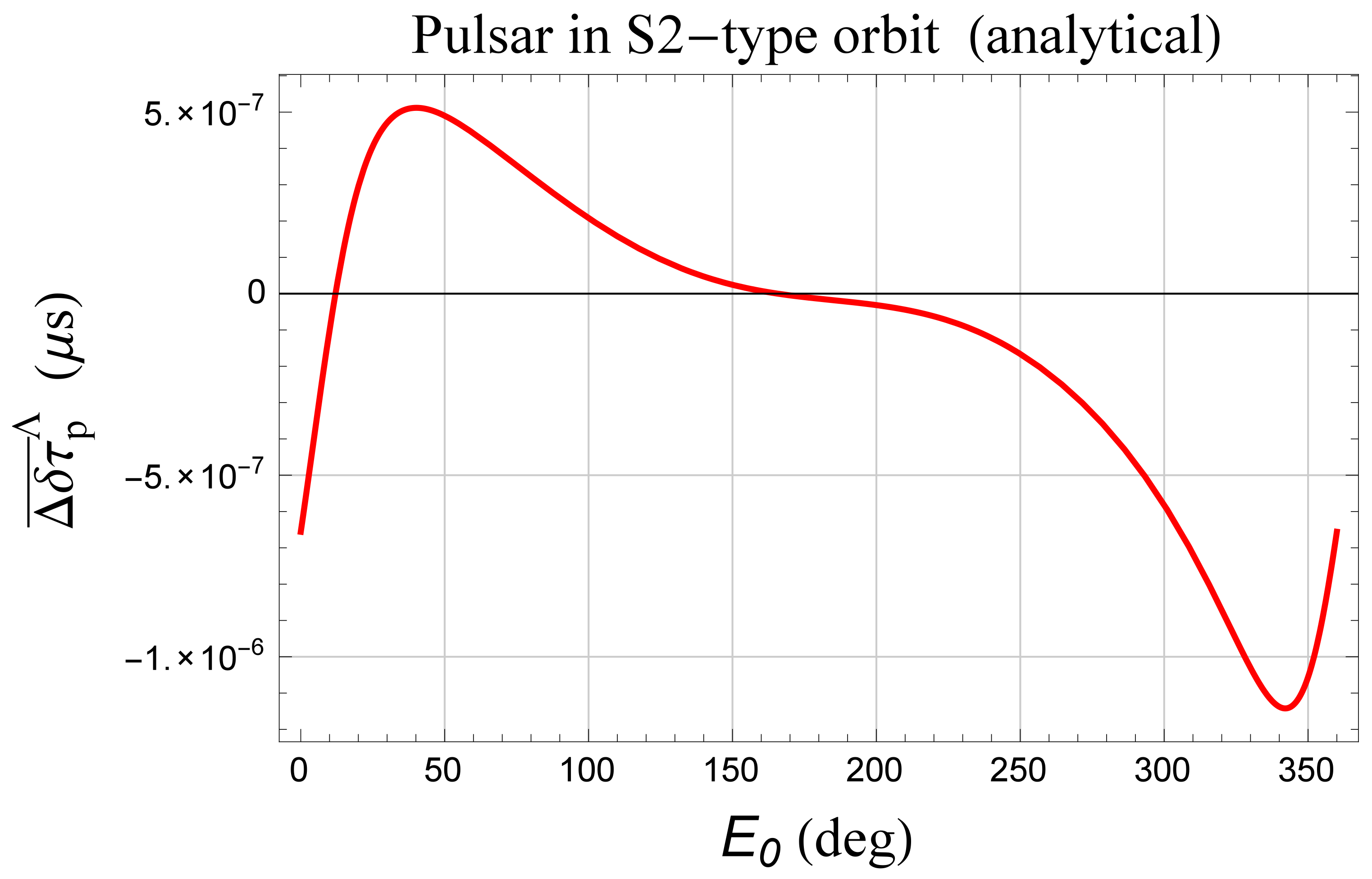
In order to explore the opportunity offered by our results to effectively constrain the CC with pulsar timing in the GC, let us consider a putative pulsar whose orbital period $P_{\mathrm{b}}$ is short enough to allow to monitor at least one full revolution during a timing campaign. In this case, by suitably choosing the initial orbital phase $E_0$, it would be possible to profitably use Equation (27) in order to maximize it; indeed, in principle, Equation (27) can even vanish. To this aim, for the sake of concreteness, let us assume a S2-type orbital configuration characterized by $P_{\mathrm{b}}=16\mathrm{yr},e=0.8839$ [73]. It turns out that the maximum of the absolute value of Equation (27) occurs for $E_0=342.08\mathrm{deg}$, which corresponds to almost an orbital period after the time of periastron passage, yielding an upper bound on the CC as little as

$$\left|\mathsf{\Lambda }\right|\lesssim 9\times {10}^{-47}{\mathrm{m}}^{-2}\left(\lesssim 2\times {10}^{-116}\mathrm{in}\mathrm{Planck}\mathrm{units}\right),$$

(28)

for a timing accuracy of ${\sigma }_{{\tau }_{\mathrm{p}}}\simeq 1\mathsf{\mu }\mathrm{s}$. It should be noted that Equation (28) is 3–4 orders magnitude better than the (likely optimistic) planetary bounds of Equations (5)–(7). Figure A1 depicts the plot of Equation (27) as a function of $E_0$. If we modify some of the parameters of the pulsar’s orbital configuration by adopting, say, $P_{\mathrm{b}}=30\mathrm{yr},e=0.987,I=90\mathrm{deg}$, it is possible to improve the bound on the CC to the level

$$\left|\mathsf{\Lambda }\right|\lesssim 4\times {10}^{-48}{\mathrm{m}}^{-2}\left(\lesssim 1\times {10}^{-117}\mathrm{in}\mathrm{Planck}\mathrm{units}\right),$$

(29)

for $E_0=354.04\mathrm{deg}$. About the figures in Equations (28)–(29), inferred by considering only ${\sigma }_{{\tau }_{\mathrm{p}}}$ as source of observational error, it must be stressed that they should be regarded with caution as preliminary and just indicative of the potential of the approach proposed. If not explicitly modeled and simultaneously estimated in actual pulsar timing data reductions, the CC-induced signature may be partially removed from the resulting residual. As such, the resulting bounds may be weaker than those in Equations (28)–(29). Further dedicated analyses should be made by simulating observations and fitting a full orbital model to them in order to assess how good the input values are recovered. A possible source of systematic uncertainty is represented by the mismodelled part of the competing averaged orbital time shifts induced by the standard post-Newtonian (pN) effects due to the current experimental errors in the SMBH’s parameters entering their formulas. For example, according to Equation (35) of Iorio [63], the amplitude of the 1pN gravitoelectric average time shift ${\overline{\Delta \delta \tau }}_{\mathrm{p}}^{\mathrm{GE}}$ is proportional to ${\mu }_{•}{c}^{-3}=22\mathrm{s}$, while the mass of the SMBH is currently known at a $\simeq 7\%$ level of accuracy [73]. Analogous considerations hold for the Lense–Thirring (Equation (51) of Iorio [63]) and quadrupole (Equation (83) of Iorio [63]) average shifts. In principle, such an issue could be circumvented if N pulsars j with different orbital configurations will be discovered. Indeed, in this case, it could be possible to write down for each of them an analytical expression

$${\overline{\Delta \delta \tau }}_j^{\exp }={\overline{\Delta \delta \tau }}_j^{\mathrm{GE}}+{\overline{\Delta \delta \tau }}_j^{\mathrm{LT}}+{\overline{\Delta \delta \tau }}_j^{Q_2}+{\overline{\Delta \delta \tau }}_j^{\mathsf{\Lambda }},j=1,2,\dots N$$

(30)

for their measured average orbital time shift ${\overline{\Delta \delta \tau }}_j^{\exp }$ as a sum of the pN terms plus the CC one by treating ${\mu }_{•},S_{•},Q_2^{•},\mathsf{\Lambda }$, which enter each term of Equation (30) as multiplicative scaling parameters, as unknowns of the resulting linear system of algebraic equations. Solving for them, it would be possible to obtain, among other things, an expression for $\mathsf{\Lambda }$ independent, by construction, of the mismodeled SMBH’s physical parameters. Such an approach could be extended also to other dynamical effects impacting the pulsar’s average orbital time shift like, e.g., third-body perturbations.

Recently, the upper bound

$$\left|{\dot{\omega }}_{\mathrm{S}2}\right|\lesssim 1.6\times {10}^{-3}{\mathrm{yr}}^{-1}=9.2{\mathrm{deg}\mathrm{cty}}^{-1}$$

(31)

on the periastron precession of the real star S2 was inferred in Hees et al. [74]. By combining Equation (31) with the well known analytical expression for the $\mathsf{\Lambda }$-induced pericenter precession (see the references cited in Section 1)

$${\dot{\omega }}_{\mathsf{\Lambda }}=\frac{1}{2}\left(\frac{\mathsf{\Lambda }{c}^2}{n_{\mathrm{b}}}\right)\sqrt{1-e^2},$$

(32)

it is possible to infer a tentative upper limit on the CC of the order of

$$\left|\mathsf{\Lambda }\right|\lesssim 3\times {10}^{-35}{\mathrm{m}}^2\left(\lesssim 8\times {10}^{-105}\mathrm{in}\mathrm{Planck}\mathrm{units}\right).$$

(33)

For much more distant pulsars, major sources of systematic uncertainty would be given by the still poorly mass background and the difficulty of effectively constraining the parameters of extremely wide orbits [75] and of the Black Hole itself over a relatively short observational time interval $\Delta T$ with respect to the expected extremely long orbital period $P_{\mathrm{b}}$ of the neutron star.

4. Summary and Conclusions

In this paper, we analytically calculated the perturbation $\Delta \delta {\tau }_{\mathrm{p}}^{\mathsf{\Lambda }}$ induced by the CC $\mathsf{\Lambda }$ on the orbital part of the time variation $\delta {\tau }_{\mathrm{p}}$ of a hypothetical pulsar p orbiting the SMBH in Sgr A${}^{\ast }$. We did not restrict to any particular orbital configuration, and our results are, thus, exact with respect to the eccentricity e; it is an important feature since most of the main sequence stars discovered so far in the GC move along highly eccentric orbits. We obtained both the instantaneous change $\Delta \delta {\tau }_{\mathrm{p}}^{\mathsf{\Lambda }}\left(E\right)$ and the net shift per orbit ${\overline{\Delta \delta \tau }}_{\mathrm{p}}^{\mathsf{\Lambda }}$: they are proportional to $c\mathsf{\Lambda }{a}^{4}sinI{\mu }_{•}^{-1}$. A distinctive feature of both of them is their explicit dependence on the initial value $E_0$ of the orbital phase. Our results hold also for a wide class of long-range modified models of gravity generating an extra-potential quadratic in the distance r.

We applied our results to some putative scenarios by adopting, for the sake of definiteness, the orbital configurations of one actually existing main sequence star orbiting Sgr A${}^{\ast }$. By considering a S2-type orbit with $P_{\mathrm{b}}=16\mathrm{yr}$, it is meaningful to look at the averaged time shift ${\overline{\Delta \delta \tau }}_{\mathrm{p}}^{\mathsf{\Lambda }}$. It turns out that, for a careful choice of the initial orbital phase $E_0$, it would be possible, in principle, to infer an upper bound $\left|\mathsf{\Lambda }\right|\lesssim 9\times {10}^{-47}{\mathrm{m}}^{-2}$ , corresponding to $\lesssim 2\times {10}^{-116}$ in Planck units, by assuming a pulsar timing accuracy of ${\sigma }_{{\tau }_{\mathrm{p}}}\simeq 1\mathsf{\mu }\mathrm{s}$. It would be 3–4 orders of magnitude better than the current, likely optimistic, constraints from Solar System’s planetary orbital motions. On the other hand, it should be stressed that the very same aforementioned bound on $\mathsf{\Lambda }$, derived by accounting for only ${\sigma }_{{\tau }_{\mathrm{p}}}$, may be optimistic in view of possible partial removal of the sought signature if not explicitly modeled and solved for in actual data reductions. As a suggestion for further dedicated investigations, simulating the observations and fitting a complete dynamical orbital model to them would be needed in order to assess how accurately the input values can be recovered. The bias due to the errors in the physical parameters of the SMBH entering the competing pN net shifts per orbit could be eliminated by setting up suitably designed linear combinations of the time delays measured for several pulsars. In the case of much more distant pulsars, using the orbital averaged time shift ${\overline{\Delta \delta \tau }}_{\mathrm{p}}^{\mathsf{\Lambda }}$ is unfeasible; only instantaneous values $\Delta \delta {\tau }_{\mathrm{p}}^{\mathsf{\Lambda }}\left(E\right)$ could be, in principle, measured. On the other hand, too wide and slow orbits may be impacted by the still poorly known mass background in the GC, and it would be difficult to effectively constrain the pulsar’s orbital parameters over a relatively short time interval with respect to its extremely long orbital period.

References

- Weinberg, S. The cosmological constant problem. Rev. Mod. Phys. 1989, 61, 1–23. [Google Scholar] [CrossRef]
- Carroll, S.M.; Press, W.H.; Turner, E.L. The cosmological constant. Annu. Rev. Astron. Astrophys. 1992, 30, 499–542. [Google Scholar] [CrossRef]
- Carroll, S.M. The Cosmological Constant. Living Rev. Relativ. 2001, 4, 1. [Google Scholar] [CrossRef] [PubMed]
- Peebles, P.J.; Ratra, B. The cosmological constant and dark energy. Rev. Mod. Phys. 2003, 75, 559–606. [Google Scholar] [CrossRef]
- Padmanabhan, T. Cosmological constant-the weight of the vacuum. Phys. Rep. 2003, 380, 235–320. [Google Scholar] [CrossRef]
- Carroll, S.M. Spacetime and Geometry. An Introduction to General Relativity; Addison Wesley: San Francisco, CA, USA, 2004. [Google Scholar]
- Davis, T.; Griffen, B. Cosmological constant. Scholarpedia 2010, 5, 4473. [Google Scholar] [CrossRef]
- O’Raifeartaigh, C.; O’Keeffe, M.; Nahm, W.; Mitton, S. One Hundred Years of the Cosmological Constant: from ‘Superfluous Stunt’ to Dark Energy. Eur. Phys. J. H 2018, 43, 1–45. [Google Scholar]
- Riess, A.G.; Filippenko, A.V.; Challis, P.; Clocchiatti, A.; Diercks, A.; Garnavich, P.M.; Gilliland, R.L.; Hogan, C.J.; Jha, S.; Kirshner, R.P.; et al. Observational Evidence from Supernovae for an Accelerating Universe and a Cosmological Constant. Astron. J. 1998, 116, 1009–1038. [Google Scholar] [CrossRef]
- Perlmutter, S.; Aldering, G.; Goldhaber, G.; Knop, R.A.; Nugent, P.; Castro, P.G.; Deustua, S.; Fabbro, S.; Goobar, A.; Groom, D.E.; et al. Measurements of Ω and Λ from 42 High-Redshift Supernovae. Astrophys. J. 1999, 517, 565–586. [Google Scholar] [CrossRef]
- Nesseris, S.; Perivolaropoulos, L. Testing ΛCDM with the growth function δ(a): Current constraints. Phys. Rev. D 2008, 77, 023504. [Google Scholar] [CrossRef]
- Spergel, D.N. The dark side of cosmology: Dark matter and dark energy. Science 2015, 347, 1100–1102. [Google Scholar] [CrossRef] [PubMed]
- Debono, I.; Smoot, G.F. General Relativity and Cosmology: Unsolved Questions and Future Directions. Universe 2016, 2, 23. [Google Scholar] [CrossRef]
- Seeliger, H. Über das Newton’sche Gravitationsgesetz. Astron. Nachr. 1895, 137, 129–136. [Google Scholar] [CrossRef]
- Ade, P.A.; Aghanim, N.; Arnaud, M.; Ashdown, M.; Aumont, J.; Baccigalupi, C.; Banday, A.J.; Barreiro, R.B.; Bartlett, J.G.; Bartolo, N.; et al. [Planck Collaboration] Planck 2015 results. XIII. Cosmological parameters. Astron. Astrophys. 2016, 594, A13. [Google Scholar]
- Mielke, E.W. Weak equivalence principle from a spontaneously broken gauge theory of gravity. Phys. Lett. B 2011, 702, 187–190. [Google Scholar] [CrossRef]
- Nojiri, S.; Odintsov, S.D. Introduction to modified gravity and gravitational alternative for dark energy. Int. J. Geom. Methods Mod. Phys. 2007, 4, 115–146. [Google Scholar] [CrossRef]
- Nojiri, S.; Odintsov, S.D. Modified gravity as an alternative for ΛCDM cosmology. J. Phys. A Math. Gen. 2007, 40, 6725–6732. [Google Scholar] [CrossRef]
- Dunsby, P.K.S.; Elizalde, E.; Goswami, R.; Odintsov, S.; Saez-Gomez, D. ΛCDM universe in f(R) gravity. Phys. Rev. D 2010, 82, 023519. [Google Scholar] [CrossRef]
- De Felice, A.; Tsujikawa, S. f(R) Theories. Living Rev. Relativ. 2010, 13, 3. [Google Scholar] [CrossRef] [PubMed]
- Nojiri, S.; Odintsov, S.D. Non-Singular Modified Gravity Unifying Inflation with Late-Time Acceleration and Universality of Viscous Ratio Bound in F(R) Theory. Prog. Theor. Phys. Supp. 2011, 190, 155–178. [Google Scholar] [CrossRef]
- Capozziello, S.; de Laurentis, M. Extended Theories of Gravity. Phys. Rep. 2011, 509, 167–321. [Google Scholar] [CrossRef]
- Clifton, T.; Ferreira, P.G.; Padilla, A.; Skordis, C. Modified gravity and cosmology. Phys. Rep. 2012, 513, 1–189. [Google Scholar] [CrossRef]
- Capozziello, S.; De Laurentis, M. The dark matter problem from f(R) gravity viewpoint. Ann. Phys. Berlin 2012, 524, 545–578. [Google Scholar] [CrossRef]
- Capozziello, S.; Harko, T.; Koivisto, T.; Lobo, F.; Olmo, G. Hybrid Metric-Palatini Gravity. Universe 2015, 1, 199–238. [Google Scholar] [CrossRef]
- De Martino, I.; De Laurentis, M.; Capozziello, S. Constraining f(R) gravity by the Large Scale Structure. Universe 2015, 1, 123–157. [Google Scholar] [CrossRef]
- Capozziello, S.; de Laurentis, M.; Luongo, O. Connecting early and late universe by f(R) gravity. Int. J. Mod. Phys. D 2015, 24, 1541002. [Google Scholar] [CrossRef]
- Cai, Y.F.; Capozziello, S.; De Laurentis, M.; Saridakis, E.N. f(T) teleparallel gravity and cosmology. Rep. Prog. Phys. 2016, 79, 106901. [Google Scholar] [CrossRef] [PubMed]
- Einstein, A. Kosmologische Betrachtungen zur allgemeinen Relativitätstheorie. In Das Relativitätsprinzip. Fortschritte der Mathematischen Wissenschaften in Monographien; Vieweg + Teubner Verlag: Wiesbaden, Germany, 1917; pp. 142–152. [Google Scholar]
- Islam, J. The cosmological constant and classical tests of general relativity. Phys. Lett. A 1983, 97, 239–241. [Google Scholar] [CrossRef]
- Cardona, J.; Tejero, J. Can interplanetary measures bound the cosmological constant? Astrophys. J. 1998, 493, 52–53. [Google Scholar] [CrossRef]
- Rindler, W. Relativity: Special, General, and Cosmological; Oxford University Press: Oxford, UK, 2001. [Google Scholar]
- Kerr, A.; Hauck, J.; Mashhoon, B. Standard clocks, orbital precession and the cosmological constant. Class. Quantum Gravity 2003, 20, 2727–2736. [Google Scholar] [CrossRef]
- Kraniotis, G.; Whitehouse, S. Compact calculation of the perihelion precession of mercury in general relativity, the cosmological constant and Jacobi’s inversion problem. Class. Quantum Gravity 2003, 20, 4817–4835. [Google Scholar] [CrossRef]
- Iorio, L. Can solar system observations tell us something about the cosmological constant? Int. J. Mod. Phys. D 2006, 15, 473–475. [Google Scholar] [CrossRef]
- Jetzer, P.; Sereno, M. Two-body problem with the cosmological constant and observational constraints. Phys. Rev. D 2006, 73, 044015. [Google Scholar] [CrossRef]
- Kagramanova, V.; Kunz, J.; Lämmerzahl, C. Solar system effects in Schwarzschild-de Sitter space-time. Phys. Lett. B 2006, 634, 465–470. [Google Scholar] [CrossRef]
- Sereno, M.; Jetzer, P. Solar and stellar system tests of the cosmological constant. Phys. Rev. D 2006, 73, 063004. [Google Scholar] [CrossRef]
- Adkins, G.; McDonnell, J.; Fell, R. Cosmological perturbations on local systems. Phys. Rev. D 2007, 75, 064011. [Google Scholar] [CrossRef]
- Adkins, G.; McDonnell, J. Orbital precession due to central-force perturbations. Phys. Rev. D 2007, 75, 082001. [Google Scholar] [CrossRef]
- Ruggiero, M.L.; Iorio, L. Solar System planetary orbital motions and f(R) theories of gravity. J. Cosmol. Astropart. Phys. 2007, 1, 010. [Google Scholar] [CrossRef]
- Sereno, M.; Jetzer, P. Evolution of gravitational orbits in the expanding universe. Phys. Rev. D 2007, 75, 064031. [Google Scholar] [CrossRef]
- Iorio, L. Solar System Motions and the Cosmological Constant: A New Approach. Adv. Astron. 2008, 2008, 268647. [Google Scholar] [CrossRef]
- Chashchina, O.I.; Silagadze, Z.K. Remark on orbital precession due to central-force perturbations. Phys. Rev. D 2008, 77, 107502. [Google Scholar] [CrossRef]
- Iorio, L.; Saridakis, E.N. Solar system constraints on f(T) gravity. Mon. Not. R. Astron. Soc. 2012, 427, 1555–1561. [Google Scholar] [CrossRef]
- Arakida, H. Note on the Perihelion/Periastron Advance Due to Cosmological Constant. Int. J. Theor. Phys. 2013, 52, 1408–1414. [Google Scholar] [CrossRef]
- Xie, Y.; Deng, X.M. f (T) gravity: Effects on astronomical observations and Solar system experiments and upper bounds. Mon. Not. R. Astron. Soc. 2013, 433, 3584–3589. [Google Scholar] [CrossRef]
- Iorio, L.; Radicella, N.; Ruggiero, M.L. Constraining f(T) gravity in the Solar System. J. Cosmol. Astropart. Phys. 2015, 8, 021. [Google Scholar] [CrossRef]
- Ovcherenko, S.S.; Silagadze, Z.K. Comment on perihelion advance due to cosmological constant. Ukr. J. Phys. 2016, 61, 342–344. [Google Scholar] [CrossRef]
- Kottler, F. Über die physikalischen Grundlagen der Einsteinschen Gravitationstheorie. Ann. Phys. Berlin 1918, 361, 401–462. [Google Scholar] [CrossRef]
- Stuchlík, Z.; Hledík, S. Some properties of the Schwarzschild-de Sitter and Schwarzschild-anti-de Sitter spacetimes. Phys. Rev. D 1999, 60, 044006. [Google Scholar] [CrossRef]
- Fienga, A.; Laskar, J.; Kuchynka, P.; Manche, H.; Desvignes, G.; Gastineau, M.; Cognard, I.; Theureau, G. The INPOP10a planetary ephemeris and its applications in fundamental physics. Celest. Mech. Dyn. Astron. 2011, 111, 363–385. [Google Scholar] [CrossRef] [Green Version]
- Hees, A.; Folkner, W.M.; Jacobson, R.A.; Park, R.S. Constraints on modified Newtonian dynamics theories from radio tracking data of the Cassini spacecraft. Phys. Rev. D 2014, 89, 102002. [Google Scholar] [CrossRef]
- Iorio, L.; Ruggiero, M.L.; Radicella, N.; Saridakis, E.N. Constraining the Schwarzschild-de Sitter solution in models of modified gravity. Phys. Dark Univ. 2016, 13, 111–120. [Google Scholar] [CrossRef]
- Hees, A.; Lamine, B.; Reynaud, S.; Jaekel, M.T.; Le Poncin-Lafitte, C.; Lainey, V.; Füzfa, A.; Courty, J.M.; Dehant, V.; Wolf, P. Radioscience simulations in general relativity and in alternative theories of gravity. Class. Quantum Gravity 2012, 29, 235027. [Google Scholar] [CrossRef] [Green Version]
- Pfahl, E.; Loeb, A. Probing the Spacetime around Sagittarius A* with Radio Pulsars. Astrophys. J. 2004, 615, 253–258. [Google Scholar] [CrossRef]
- Zhang, F.; Lu, Y.; Yu, Q. On the Existence of Pulsars in the Vicinity of the Massive Black Hole in the Galactic Center. Astrophys. J. 2014, 784, 106. [Google Scholar] [CrossRef]
- Chennamangalam, J.; Lorimer, D.R. The Galactic Centre pulsar population. Mon. Not. R. Astron. Soc. Lett. 2014, 440, L86–L90. [Google Scholar] [CrossRef]
- Rajwade, K.M.; Lorimer, D.R.; Anderson, L.D. Detecting pulsars in the Galactic Centre. Mon. Not. R. Astron. Soc. 2017, 471, 730–739. [Google Scholar] [CrossRef]
- Psaltis, D.; Wex, N.; Kramer, M. A Quantitative Test of the No-hair Theorem with Sgr A* Using Stars, Pulsars, and the Event Horizon Telescope. Astrophys. J. 2016, 818, 121. [Google Scholar] [CrossRef]
- Goddi, C.; Falcke, H.; Kramer, M.; Rezzolla, L.; Brinkerink, C.; Bronzwaer, T.; Davelaar, J.R.J.; Deane, R.; de Laurentis, M.; Desvignes, G.; et al. BlackHoleCam: Fundamental physics of the galactic center. Int. J. Mod. Phys. D 2017, 26, 1730001. [Google Scholar] [CrossRef]
- Espriu, D. Pulsar timing arrays and the cosmological constant. AIP Conf. Proc. 2014, 1606, 86–98. [Google Scholar]
- Iorio, L. Post-Keplerian perturbations of the orbital time shift in binary pulsars: An analytical formulation with applications to the galactic center. Eur. Phys. J. C 2017, 77, 439. [Google Scholar] [CrossRef]
- Schücker, T.; Zaimen, N. Cosmological constant and time delay. Astron. Astrophys. 2008, 484, 103–106. [Google Scholar] [CrossRef]
- Merritt, D.; Alexander, T.; Mikkola, S.; Will, C.M. Stellar dynamics of extreme-mass-ratio inspirals. Phys. Rev. D 2011, 84, 044024. [Google Scholar] [CrossRef]
- Sadeghian, L.; Will, C.M. Testing the black hole no-hair theorem at the galactic center: Perturbing effects of stars in the surrounding cluster. Class. Quantum Gravity 2011, 28, 225029. [Google Scholar] [CrossRef]
- Angélil, R.; Saha, P. Clocks around Sgr A*. Mon. Not. R. Astron. Soc. 2014, 444, 3780–3791. [Google Scholar] [CrossRef]
- Zhang, F.; Iorio, L. On the Newtonian and Spin-induced Perturbations Felt by the Stars Orbiting around the Massive Black Hole in the Galactic Center. Astrophys. J. 2017, 834, 198. [Google Scholar] [CrossRef]
- Zhang, F.; Saha, P. Probing the spinning of the massive black hole in the Galactic Center via pulsar timing: A Full Relativistic Treatment. Astrophys. J. 2017, 849, 33. [Google Scholar] [CrossRef]
- De Laurentis, M.; Younsi, Z.; Porth, O.; Mizuno, Y.; Rezzolla, L. Test-particle dynamics in general spherically symmetric black hole spacetimes. arXiv, 2017; arXiv:1712.00265. [Google Scholar]
- Casotto, S. Position and velocity perturbations in the orbital frame in terms of classical element perturbations. Celest. Mech. Dyn. Astron. 1993, 55, 209–221. [Google Scholar] [CrossRef]
- Eckart, A.; Hüttemann, A.; Kiefer, C.; Britzen, S.; Zajaček, M.; Lämmerzahl, C.; Stöckler, M.; Valencia-S, M.; Karas, V.; García-Marín, M. The Milky Way’s Supermassive Black Hole: How Good a Case Is It? Found. Phys. 2017, 47, 553–624. [Google Scholar] [CrossRef]
- Gillessen, S.; Plewa, P.M.; Eisenhauer, F.; Sari, R.; Waisberg, I.; Habibi, M.; Pfuhl, O.; George, E.; Dexter, J.; von Fellenberg, S.; et al. An Update on Monitoring Stellar Orbits in the Galactic Center. Astrophys. J. 2017, 837, 30. [Google Scholar] [CrossRef]
- Hees, A.; Do, T.; Ghez, A.M.; Martinez, G.D.; Naoz, S.; Becklin, E.E.; Boehle, A.; Chappell, S.; Chu, D.; Dehghanfar, A.; et al. Testing General Relativity with Stellar Orbits around the Supermassive Black Hole in Our Galactic Center. Phys. Rev. Lett. 2017, 118, 211101. [Google Scholar] [CrossRef] [PubMed]
- Lucy, L.B. Mass estimates for visual binaries with incomplete orbits. Astron. Astrophys. 2014, 563, A126. [Google Scholar] [CrossRef]
- Brumberg, V.A. Essential Relativistic Celestial Mechanics; Taylor & Francis Group: Boca Raton, FL, USA, 1991. [Google Scholar]
- Milani, A.; Nobili, A.; Farinella, P. Non-Gravitational Perturbations and Satellite Geodesy; Taylor & Francis: Boca Raton, FL, USA, 1987. [Google Scholar]
- Soffel, M.H. Relativity in Astrometry, Celestial Mechanics and Geodesy; Springer: Berlin, Germany, 1989. [Google Scholar]
- Bertotti, B.; Farinella, P.; Vokrouhlický, D. Physics of the Solar System—Dynamics and Evolution, Space Physics, and Spacetime Structure; Springer: Dordrecht, The Netherlands, 2003. [Google Scholar]
© 2018 by the author. Licensee MDPI, Basel, Switzerland. This article is an open access article distributed under the terms and conditions of the Creative Commons Attribution (CC BY) license (http://creativecommons.org/licenses/by/4.0/).
Share and Cite
MDPI and ACS Style
Iorio, L. Perspectives on Constraining a Cosmological Constant-Type Parameter with Pulsar Timing in the Galactic Center. Universe 2018, 4, 59. https://0-doi-org.brum.beds.ac.uk/10.3390/universe4040059
AMA Style
Iorio L. Perspectives on Constraining a Cosmological Constant-Type Parameter with Pulsar Timing in the Galactic Center. Universe. 2018; 4(4):59. https://0-doi-org.brum.beds.ac.uk/10.3390/universe4040059
Chicago/Turabian StyleIorio, Lorenzo. 2018. "Perspectives on Constraining a Cosmological Constant-Type Parameter with Pulsar Timing in the Galactic Center" Universe 4, no. 4: 59. https://0-doi-org.brum.beds.ac.uk/10.3390/universe4040059
Note that from the first issue of 2016, this journal uses article numbers instead of page numbers. See further details here.