Passive Advection of a Vector Field by Compressible Turbulent Flow: Renormalizations Group Analysis near d = 4 ^†

Abstract

The renormalization group approach and the operator product expansion technique are applied to the model of a passively advected vector field by a turbulent velocity field. The latter is governed by the stochastic Navier-Stokes equation for a compressible fluid. The model is considered in the vicinity of space dimension $d=4$ and the perturbation theory is constructed within a double expansion scheme in y and $\epsilon =4-d$, where y describes scaling behaviour of the random force that enters the Navier-Stokes equation. The properties of the correlation functions are investigated, and anomalous scaling and multifractal behaviour are established. All calculations are performed in the leading order of y, $\epsilon$ expansion (one-loop approximation).

1. Introduction

Many phenomena in the nature are associated with hydrodynamic flows. Ranging from microscopic up to macroscopic spatial scales, fluids can exist in very different states. Especially intriguing behaviour is observed for turbulent flows; moreover, such flows are rather a rule than an exception [1,2]. Despite the vast amount of effort that has been put into investigation of turbulence, fundamental properties of the underlying Navier-Stokes equation remain unsolved. The most intriguing one is intermittency. Being an irregular alternation of phases of certain dynamics, it means that very rare configurations of a system contribute most significally to statistical distributions. This leads to anomalous scaling, which manifests itself in singular (usually power-like) behavior of various statistical quantities as functions of the integral turbulence scales, with infinite sets of independent anomalous exponents [1,2].

In astrophysical applications, turbulence is an ubiquitous phenomenon [3,4]; moreover, we usually have to deal with a compressible fluid rather than incompressible one [4,5,6,7,8]. In this work, our aim is to look closely at a compressible turbulence [9], motivated by the previous studies [10,11,12,13,14,15,16,17,18,19] of the incompressible case and the need for an astrophysical description of a squishy medium.

A quantitative parameter that describes “intensity” of turbulent motion is the so-called Reynolds number $\mathrm{Re}$, which represents a dimensionless ratio between inertial and dissipative forces. The fully developed turbulence (i.e., the fluid motion with $\mathrm{Re}\gg 1$) is characterized by existence of an inertial range—an interval of scales in which both the input and dissipation of energy are insignificant, and the only notable dynamical process is the re-distribution of energy along the spectrum. Therefore, one expects the inertial range to be governed by simple (and possibly universal) laws describing turbulent processes. In accordance with this hypothesis, the classical Kolmogorov-Obukhov theory assumes that statistical characteristics of a system, i.e., its correlation and response functions, do not depend on either the internal (l, viscosity-related) or the external (L, external force-related) scales [1,2]. Nevertheless, correlation functions can depend on the external scale due to certain kinematic effects—for example, the sweeping effect, in which small turbulent eddies are carried by large ones as a whole without distortion. Experimental studies confirm this: In most cases, measurable quantities contain some dependence on large scale L, which is usually singular and is described by an infinite set of anomalous exponents—a phenomenon referred to as “anomalous scaling” and “multiscaling” [20].

Within the framework of numerous semi-heuristic models, the anomalous exponents are related to statistical properties of the local dissipation rate, the fractal (Haussdorf) dimension of structures formed by the small-scale turbulent eddies, the characteristics of nontrivial structures (vortex filaments), and so on [1,2]. The common drawback of such models is that they are only loosely related to underlying hydrodynamical equations, involve arbitrary adjusting parameters and, therefore, cannot be considered to be the basis for construction of a systematic perturbation theory in certain small (at least formal) expansion parameter.

When solving the problem, the renormalization group method accompanied by the operator product expansion (OPE) was applied; see the monographs [21,22,23,24]. The renormalization group (RG) method performs a certain rearrangement (infinite resummation) of the original perturbation series, and turns them into a series of the parameter of order unity (since we deal with fully developed turbulence, where $\mathrm{Re}$ tends to infinity, it is unpossible to work with initial “naive” perturbation expansion). In the theory of critical phenomena that parameter is $\epsilon =4-d$, the deviation of the dimensionality of space d from its upper critical value, hence the term “epsilon expansion”. Such expansions are still divergent, but they allow one to prove the existence of infrared (IR) scaling behavior (if such exists) and to systematically calculate the corresponding dimensions as series in $\epsilon$.

For the Navier-Stokes turbulence, the situation is much more difficult. Besides the RG expansion parameter y is not small and the RG series are divergent, due to the sweeping effect and anomalous scaling, the perturbation diagrams have strong divergences at $L\to \infty$. Adequate analysis of these issues takes one far beyond the standard RG method and should be combined with the short-distance operator product expansion.

One of the greatest challenges is an investigation of the Navier-Stokes equation for a compressible fluid, and, in particular, a passive scalar field advection by this velocity ensemble. Several decades ago, the first study was carried out for a passively advected scalar field; see [25,26] and review paper [20]. Further research in this area was devoted to more realistic generalizations [11,12,13,14,15,16,17,18,19,27,28,29,30,31]. The approach of RG+OPE was also applied to more sophisticated cases, in particular, to the one of compressible fluid [32,33,34,35,36,37,38,39,40,41].

This paper is a continuation of our previous works [42,43,44,45] and is organized as follows. In the introductory Section 2 we give a brief overview of the model. In Section 3 we reformulate stochastic equations into field-theoretical language. Section 4 is devoted to the renormalization group analysis. In Section 5 we present the fixed points’ structure and describes possible scaling regimes. In Section 6 critical dimensions of composite fields are calculated. In Section 7 OPE is applied to the equal-time structure functions constructed of the vector fields; the anomalous exponents are calculated. The concluding Section 8 is devoted to a brief discussion.

2. Model

Let us start with a brief discussion of a model for compressible velocity fluctuations. The dynamics of a compressible fluid is governed by the Navier-Stokes equation [46]:

$$\rho {\nabla }_t{v}_i={\nu }_0[{\delta }_{ik}{\partial }^2-{\partial }_i{\partial }_k]v_k+{\mu }_0{\partial }_i{\partial }_k{v}_k-{\partial }_{i}p+f_i^v,$$

(1)

where the operator ${\nabla }_t$ denotes an expression ${\nabla }_t={\partial }_t+v_k{\partial }_k$, also known as a Lagrangian (or convective) derivative. Further, $\rho =\rho (t,\mathit{x})$ is a fluid density field, $v_i=v_i(t,\mathit{x})$ is the velocity field, ${\partial }_t=\partial /\partial t$, ${\partial }_i=\partial /\partial x_i$, ${\partial }^2={\partial }_i{\partial }_i$ is the Laplace operator, $p=p(t,\mathit{x})$ is the pressure field, and $f_i^v$ is the external force, which is specified later. In what follows we employ a condensed notation in which we write $x=(t,\mathit{x})$, where a spatial variable $\mathit{x}$ equals $(x_1,x_2,\dots ,x_d)$ with d being a dimensionality of space. Two parameters ${\nu }_0$ and ${\mu }_0$ are two viscosity coefficients [46]. Summations over repeated vector indices (Einstein summation convention) are always implied in this work. In subsequent sections we employ the RG method, in which it is necessary to distinguish between unrenormalized (bare) and renormalized parameters. The former we denote by a subscript “0”.

Equation (1) has to be augmented by two additional relations, which are a continuity equation and a certain thermodynamic relation [46]. The former can be written in the form

$${\partial }_t\rho +{\partial }_i\left(\rho v_i\right)=0$$

(2)

and the latter we choose as follows

$$\delta p=c_0^2\delta \rho .$$

(3)

Here $\delta p$ and $\delta \rho$ are deviations from the equilibrium values of pressure field and density field, respectively.

Viscous terms in Equation (1) characterize dissipative processes in the system and are especially important at small spatial scales. Without a continuous input of energy, turbulent processes would eventually die out and the flow would become regular. There are various possibilities for modelling of energy input [23]. For translationally invariant theories it is convenient to specify properties of the random force $f_i$ in frequency-momentum representation

$$\langle f_i(t,\mathit{x})f_j(t^{\prime },{\mathit{x}}^{\prime })=\frac{\delta (t-t^{\prime })}{{\left(2\pi \right)}^d}{\int }_{k>m}{\mathrm{d}}^{d}k{D}_{ij}^v\left(\mathit{k}\right){\mathrm{e}}^{i\mathit{k}·\left(\mathit{x}-{\mathit{x}}^{\prime }\right)},$$

(4)

where the delta function ensures Galilean invariance of the model. The integral in Equation (4) is infrared (IR) regularized with a parameter $m\sim L_v^{-1}$, where $L_v$ denotes outer scale, i.e., scale of the biggest turbulent eddies. More details can be found in the literature [23]. The kernel function $D_{ij}^v\left(\mathit{k}\right)$ is now chosen in the following form

$$D_{ij}^v\left(\mathit{k}\right)=g_{10}{\nu }_0^3{k}^{4-d-y}\{P_{ij}\left(\mathit{k}\right)+\alpha Q_{ij}\left(\mathit{k}\right)\}+g_{20}{\nu }_0^3{\delta }_{ij}$$

(5)

that consists of two terms. The term proportional to the charge $g_{10}$ is non-local and ensures a steady input of energy into the system from outer scales. The value of the scaling exponent y describes a deviation from a logarithmic behaviour. In the stochastic theory of turbulence, the main interest is in the limit behaviour $y\to 4$ that yields an ideal pumping from infinite spatial scales [23]. The projection operators $P_{ij}$ and $Q_{ij}$ in the momentum space read

$$P_{ij}\left(\mathit{k}\right)={\delta }_{ij}-\frac{k_i{k}_j}{k^2},Q_{ij}=\frac{k_i{k}_j}{k^2}$$

(6)

and correspond to the transversal and longitudinal projector, respectively, $k=\left|\mathit{k}\right|$ is the wave number.

In what follows, we heavily rely on a powerful methods of RG framework. The local term proportional to $g_{20}$ in (6) is not dictated by the physical considerations, but by a proper renormalization treatment [45]. Let us briefly describe this subtle point. An important difference of the present study with the traditional approaches [23,47] is a special role of the space dimension $d=4$. Usually the spatial dimension d plays a passive role and is considered only as an independent parameter. However, Honkonen and Nalimov [48] showed that in the vicinity of space dimension $d=2$ additional divergences appear in the model of the incompressible Navier-Stokes ensemble, and these divergences have to be properly taken into account. Their procedure also results into improved perturbation expansion [49,50]. As we see in the next section a similar situation occurs for the model (1) in the vicinity of space dimension $d=4$. Here in the 1-irreducible Green function ${〈v^{\prime }{v}^{\prime }〉}_{1-\mathrm{ir}}$ an additional divergence appears. In this particular case, it is necessary to apply the technique of double expansion. The parameteres of the expansion are y, which describes the scaling behaviour of a random force, and $\epsilon =4-d$, i.e., the deviation from the space dimension $d=4$ [31,48]. As we will see, application of such double expansion leads to some infinite resummation of the ordinary y expansion near physically interesting dimension $d=3$ and improve answers for critical dimensions, especially their behavior at large values of $\alpha$.

The stochastic approach to magnetohydrodynamics is based on the following equation

$${\partial }_t{\theta }_i+{\partial }_k(v_k{\theta }_i-v_i{\theta }_k)={\kappa }_0{\partial }^2{\theta }_i+f_i^{\theta },$$

(7)

where ${\kappa }_0$ stands for the magnetic diffusion coefficient. For a detailed exposition we recommend textbook [4]; the quantity ${\theta }_i={\theta }_i\left(x\right)$ is the fluctuating part of the total magnetic field.

Random force $f_i^{\theta }\equiv f_i^{\theta }\left(x\right)$ is again assumed to be a Gaussian variable with zero mean and given covariance,

$$\langle f_i^{\theta }\left(x\right)f_j^{\theta }\left(x^{\prime }\right)\rangle =\delta (t-t^{\prime })C_{ij}(\mathit{r}/L_{\theta }),\mathit{r}=\mathit{x}-{\mathit{x}}^{\prime },$$

(8)

where $C_{ij}(\mathit{r}/L_{\theta })$ is a certain function finite at limit $(\mathit{r}/L_{\theta })\to 0$ and rapidly decaying for $(\mathit{r}/L_{\theta })\to \infty$.

3. Quantum Field Theory Formulation

Our main theoretical tool is the renormalization group theory. Its proper application requires a proof of a renormalizability of the model, i.e., a proof that only a finite number of divergent structures exists in a diagrammatic expansion [22]. This requirement can be accomplished by the following procedure: First the stochastic Equation (1) is divided by density field $\rho$, then fluctuations in viscous terms are neglected, and, finally, using the expressions (2) and (3), the problem might be reformulated into a system of two coupled equations

$$\begin{array}{cc}\hfill {\nabla }_t{v}_i& ={\nu }_0[{\delta }_{ik}{\partial }^2-{\partial }_i{\partial }_k]v_k+{\mu }_0{\partial }_i{\partial }_k{v}_k-{\partial }_i\varphi +f_i,\hfill \end{array}$$

(9)

$$\begin{array}{cc}\hfill {\nabla }_t\varphi & =-c_0^2{\partial }_i{v}_i,\hfill \end{array}$$

(10)

where a new field $\varphi =\varphi \left(x\right)$ has been introduced and it is related to the density fluctuations via the relation $\varphi =c_0^{2}ln(\rho /\overline{\rho })$ [45]. Here, a parameter $c_0$ denotes the adiabatic speed of sound, $\overline{\rho }$ is the mean value of $\rho$, and $f_i=f_i\left(x\right)$ is the external force normalized per unit mass.

According to the general theorem [21,22], the stochastic problem given by Equations (7), (9), and (10) is equivalent to the field theoretic model with a doubled set of fields $\Phi =\left\{v_i,v_i^{\prime },\varphi ,{\varphi }^{\prime }\right\}$ and De Dominicis-Janssen action functional. The latter can be written in a compact form as a sum of two terms

$$\begin{array}{cc}\hfill S_{\mathrm{total}}[\Phi ]& =S_{\mathrm{vel}}[\Phi ]+S_{\mathrm{mag}}[\Phi ],\hfill \end{array}$$

(11)

where the first term describes a velocity part

$$\begin{array}{cc}\hfill S_{\mathrm{vel}}[\Phi ]& =\frac{v_i^{\prime }{D}_{ij}^v{v}_j^{\prime }}{2}+v_i^{\prime }[-{\nabla }_t{v}_i+{\nu }_0({\delta }_{ij}{\partial }^2-{\partial }_i{\partial }_j)v_j+u_0{\nu }_0{\partial }_i{\partial }_j{v}_j-{\partial }_i\varphi ]\hfill \\ & +{\varphi }^{\prime }[-{\nabla }_t\varphi +v_0{\nu }_0{\partial }^2\varphi -c_0^2\left({\partial }_i{v}_i\right)].\hfill \end{array}$$

(12)

Here, $D_{ij}^v$ is the correlation function (5). Note that we have introduced a new dimensionless parameter $u_0={\mu }_0/{\nu }_0>0$ and a new term $v_0{\nu }_0{\varphi }^{\prime }{\partial }^2\varphi$ with another positive dimensionless parameter $v_0$, which is needed to ensure multiplicative renormalizability. Due to succession reason we denote this amplitude parameter with the same letter as velocity field $v_i$; however, since it is a scalar quantity unlike the velocity field and since it plays completely another role we hope that this denotation will not mislead the reader.

The second term in Equation (11) reads

$$S_{\mathrm{mag}}[\Phi ]=\frac{1}{2}{\theta }_i^{\prime }{D}_{ij}^{\theta }{\theta }_j^{\prime }+{\theta }_k^{\prime }[-{\partial }_t{\theta }_k-\left(v_i{\partial }_i\right){\theta }_k+\left({\theta }_i{\partial }_i\right)v_k+{\nu }_0{w}_0{\partial }^2{\theta }_k],$$

(13)

where we have introduced another dimensionless parameter $w_0$ via ${\kappa }_0={\nu }_0{w}_0$. For brevity we have not explicitly written integrals over the spatial variable $\mathit{x}$ and the time variable t in Equations (12) and (13).

In a functional formulation various stochastic quantities (correlation and structure functions) are calculated as path integrals with weight functional $exp\left(S_{\mathrm{total}}[\Phi ]\right)$. The main benefits of such approach are transparence in a perturbation theory and potential use of the powerful methods of the quantum field theory, such as Feynman diagrammatic technique and renormalization group procedure [22,23,24].

4. Renormalization Group Analysis

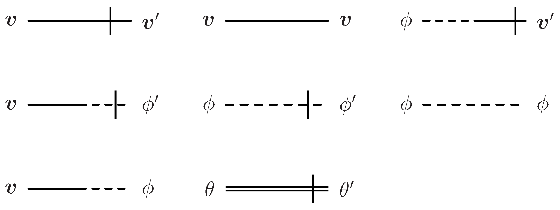
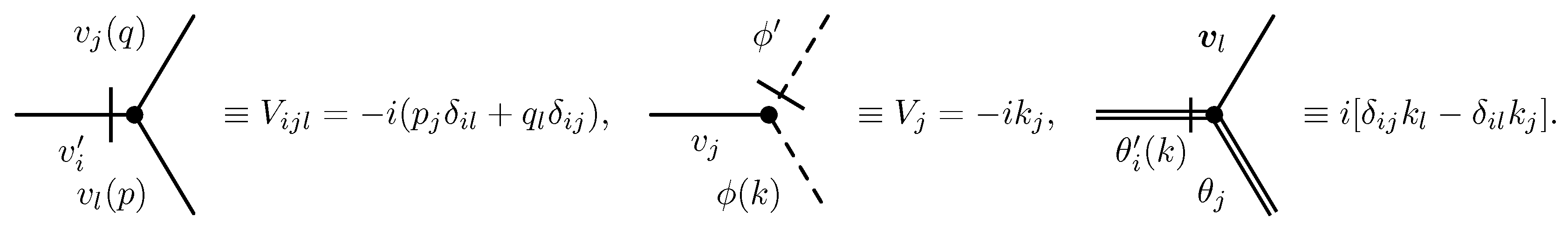
Ultraviolet renormalizability reveals itself in a presence divergences in Feynman graphs, which are constructed according to simple laws [21,24] using a graphical notation from Figure 1 and Figure 2. From a practical point of view, an analysis of the 1-particle irreducible Green functions, later referred to as 1-irreducible Green functions following the notation in Ref. [21], is of utmost importance.

Superficial UV divergences whose removal requires counterterms can be present only in those functions $\mathsf{\Gamma }$ for which the index of divergence is a non-negative integer. The only graphs that are needed to be calculated are two-point Green functions. For a velocity part, the following graphs have to be analyzed

(14)

and for a magnetic part we have one Feynman diagram

(15)

The remaining diagrams are either UV finite or the Galilean invariance prohibits their appearance. Because the calculation of the divergent parts of Feynman diagrams is rather straightforward and proceeds in the usual fashion [21,22,24], we refrain from mentioning here all the technical details. For the latter, we recommend an interested reader to consult our previous works [40,42,43,45].

Here, we just provide a result of the diagram D shown in Equation (15)

$$\begin{array}{cc}\hfill D=\frac{\overline{S_d}}{2d}{p}^2{P}_{12}\left(\mathit{p}\right)\nu & \left\{\frac{1-d}{1+w}\right[\frac{g_1}{y}(\frac{\mu }{m}{)}^y+\frac{g_2}{\epsilon }(\frac{\mu }{m}{)}^{\epsilon }]\hfill \\ & -\frac{u-w}{u(u+w)}\left[\frac{\alpha g_1}{y}\right(\frac{\mu }{m}{)}^y+\frac{g_2}{\epsilon }\left(\frac{\mu }{m}{)}^{\epsilon }\right]\},\hfill \end{array}$$

(16)

where $\overline{S_d}=S_d/{\left(2\pi \right)}^d$ with $S_d=2{\pi }^{d/2}/\mathsf{\Gamma }(d/2)$ is the surface area of the unit sphere in the $d$—dimensional space and $\mathsf{\Gamma }\left(x\right)$ is Euler’s Gamma function. The expression (16) differs from the result obtained in Ref. [40] by the presence of terms containing the charge $g_2$. Further, from (16) we directly derive renormalization constant $Z_{\kappa }$ [where $\kappa =\nu w$, see Equation (13)] and the corresponding anomalous dimension ${\gamma }_{\kappa }$.

5. Scaling Regimes

The relation between the initial and renormalized action functionals $S(\Phi ,e_0)=S^R(Z_{\Phi }\Phi ,e,\mu )$ (where $e_0$ is the complete set of bare parameters and e is the set of their renormalized counterparts) leads to the fundamental RG differential equation. Based on the analysis of this equation it follows that the large scale behaviour with respect to spatial and time scales is governed by the IR attractive (“stable”) fixed points $g^{\ast }\equiv \{g_1^{\ast },g_2^{\ast },u^{\ast },v^{\ast }\}$, whose coordinates are found from the conditions [21,22]:

$$\begin{array}{c}{\beta }_{g_1}\left(g^{\ast }\right)={\beta }_{g_2}\left(g^{\ast }\right)={\beta }_u\left(g^{\ast }\right)={\beta }_v\left(g^{\ast }\right)=0,\hfill \end{array}$$

(17)

where ${\beta }_x={\tilde{\mathcal{D}}}_{\mu }x$ is the so-called beta functions and ${\tilde{\mathcal{D}}}_{\mu }$ is the differential operation $\mu {\partial }_{\mu }$ for fixed $e_0$. The existence of IR attractive solutions of the RG equations leads to the existence of the scaling behaviour of Green functions. The type of the fixed point is determined by the matrix ${\Omega }_{ij}=\partial {\beta }_i/\partial g_j{|}_{g=g^{\ast }}$: for the IR attractive fixed points it has to be positive definite.

The character of the IR behaviour depends on the mutual relation between y and $\epsilon$—two formally small quantities which were introduced in the correlator of the random force (5) in the Navier-Stokes equation.

In work [45] the velocity part (without ${\beta }_w$) of the system (17) was analyzed. Altogether, three IR attractive fixed points, which define possible scaling regimes of the system, were found. The fixed point FPI with coordinates $g_1^{\ast }=0$ and $g_2^{\ast }=0$; the “local” fixed point FPII with coordinates $g_1^{\ast }=0$ and $g_2^{\ast }\ne 0$; and the “nonlocal” fixed point FPIII with coordinates $g_1^{\ast }\ne 0$ and $g_2^{\ast }\ne 0$.

Moreover, from the analysis in Ref. [45] it follows that for nontrivial regimes the coordinate u takes value $u^{\ast }=1$. Substituting these values together with $d=4$ we obtain for the charge w the following beta function

$${\beta }_w=\frac{w-1}{16{(1+w)}^2}[g_1(6+2\alpha +9w+3w^2)+g_2(3w^2+9w+8)].$$

(18)

Note that this result is in accordance with previous work for the passive scalar case [43] and vector case as well [51]. The only nontrivial solution for the fixed point is $w^{\ast }=1$. Also, it is rather straightforward to show that ${\partial }_w{\beta }_w>0$ at nontrivial fixed points, what ensures IR stability.

Depending on the values of y and $\epsilon$, the different values of the critical dimension for various quantities F are obtained. They can be calculated via the expression

$$\Delta \left[F\right]=d_F^k+{\Delta }_{\omega }{d}_F^{\omega }+{\gamma }_F^{\ast },$$

(19)

where $d_F^{\omega }$ is the canonical frequency dimension, $d_F^k$ is the momentum dimension, ${\gamma }_F^{\ast }$ is the anomalous dimension at the critical point (FPII or FPIII), and ${\Delta }_{\omega }=2-{\gamma }_{\nu }^{\ast }$ is the critical dimension of frequency.

6. Composite Fields

Measurable quantities are certain correlation or structure functions of composite operators. A local composite operator is polynomial constructed from the fields $\theta \left(x\right)$ at a single space-time point x (as well as from finite-order derivatives of the field $\theta \left(x\right)$). In the Green functions with such objects, new UV divergences arise and require the additional renormalization procedure [21].

The simplest case of a composite operator is the scalar operator $F\left(x\right)={\theta }^n\left(x\right)$. Here, we focus on the irreducible tensor operators of the form

$$F_{i_1\cdots i_l}^{(n,l)}={\theta }_{i_1}\cdots {\theta }_{i_l}{\left({\theta }_j{\theta }_j\right)}^s+\cdots ,$$

(20)

where l is the rank of the tensor (i.e., the number of the free vector indices), and $n=l+2s$ is the total number of the fields $\theta$ entering the operator.

For practical calculations, it is convenient to contract the tensors (20) with an arbitrary constant vector $\mathit{\lambda }=\left\{{\lambda }_i\right\}$. The resulting scalar operator takes the form

$$F^{(n,l)}={\left({\lambda }_i{w}_i\right)}^l{\left(w_i{w}_i\right)}^s+\cdots ,w_i\equiv {\theta }_i,$$

(21)

where the subtractions, denoted by the ellipsis, necessarily include the factors of ${\lambda }^2={\lambda }_i{\lambda }_i$.

In order to calculate the critical dimension of the operator we should renormalize it. The operators (20) are in fact multiplicatively renormalizable, $F^{(n,l)}=Z_{(n,l)}{F}_R^{(n,l)}$, with certain renormalization constants $Z_{(n,l)}$ (see Ref. [39]). The renormalization constants $Z_{(n,l)}$ are determined by the finiteness of the 1-irreducible Green function ${\mathsf{\Gamma }}_{nl}(x;\theta )$, which in the one-loop approximation is diagrammatically represented as

(22)

where numerical factor $1/2$ is a symmetry factor of the graph and the thick dot with two lines attached denotes the operator vertex

$$V(x;x_1,x_2)=\frac{{\delta }^2{F}^{(n,l)}}{\delta {\theta }_i\delta {\theta }_j}.$$

(23)

Divergent parf of a one-loop diagram in Equation (22) reads

(24)

and result for ${\mathsf{\Gamma }}_{nl}$ in terms of $n=l+2s$ and l is the following:

$$\begin{array}{cc}\hfill {\mathsf{\Gamma }}_{nl}(x;\theta )& =F^{(n,l)}\left(x\right)\{1-\frac{1}{4wd(d+2)}[\frac{Q_1}{(1+w)}(\frac{g_1}{y}+\frac{g_2}{\epsilon })\hfill \\ & +\frac{Q_2}{u(u+w)}(\frac{\alpha g_1}{y}+\frac{g_2}{\epsilon })\left]\right\}.\hfill \end{array}$$

(25)

The corresponding anomalous dimension ${\gamma }_{nl}$ reads

$${\gamma }_{nl}=\frac{1}{4dw(d+2)}\left\{\frac{Q_1}{1+w}(g_1+g_2)+\frac{Q_2}{u(u+w)}(\alpha g_1+g_2)\right\}.$$

(26)

To obtain the critical dimension, one needs to substitute the coordinates of the fixed points into (26) and then use the relation (19). For the fixed point FPII the critical dimension is

$${\Delta }_{nl}=\frac{n}{4}\epsilon +\frac{Q_1+Q_2}{72}\epsilon ;$$

(27)

for the fixed point FPIII it is

$${\Delta }_{nl}=\frac{n}{6}y+\frac{y}{12}\frac{Q_1(\alpha y+2y-3\epsilon )+3\alpha Q_2(y-\epsilon )}{9\left[y\right(2+\alpha )-3\epsilon ]}.$$

(28)

Both expressions (27) and (28) suppose higher order corrections in y and $\epsilon$.

The latter result for FPIII is in agreement with previously known result for the analysis near three-dimensional space $d=3$: Expanding expression (28) in y at fixed value $\epsilon =1$ (which corresponds to $d=3$) gives

$$\begin{array}{cc}\hfill {\Delta }_{nl}& =\frac{ny}{6}+\frac{y(Q_1+\alpha Q_2)}{108}+\mathcal{O}\left(y^2\right).\hfill \end{array}$$

(29)

The first two terms (proportional to y) in Equation (29) coincide with analogous expression obtained earlier in Ref. [40]. This means that expression (28), obtained as a result of the double y and $\epsilon$ expansion near $d=4$, may be considered as a certain partial infinite resummation of the ordinary y expansion. This resummation significantly improves the situation at large $\alpha$: Now we do not have the pathology when the critical dimensions ${\Delta }_{nl}$ are linear in $\alpha$ [see Equations (28) and (29)] and, therefore, grow with $\alpha$ without a bound.

7. Operator Product Expansion

Our main interest are pair correlation functions, whose unrenormalized counterparts have been defined in Equation (20). For Galilean invariant equal-time functions we can write the following representation

$$\langle F^{(m,i)}(t,\mathit{x})F^{(n,j)}(t,{\mathit{x}}^{\prime })\rangle \simeq {\mu }^{d_F}{\nu }^{d_F^{\omega }}{\left(\mu r\right)}^{-{\Delta }_{(m,i)}-{\Delta }_{(n,j)}}{\zeta }_{m,i;n,j}(mr,c\left(r\right)),$$

(30)

where $r=|\mathit{x}-{\mathit{x}}^{\prime }|$ and $c\left(r\right)$ is effective speed of sound. Its limiting behavior is

$$c\left(r\right)=c\frac{{\left(\mu r\right)}^{{\Delta }_c}}{\mu \nu }\to \left\{\begin{array}{c}c\left(0\right)\mathrm{for}\mathrm{non}-\mathrm{local}\mathrm{regime}\mathrm{FPIII};\hfill \\ c(\infty )\mathrm{for}\mathrm{local}\mathrm{regime}\mathrm{FPII},\hfill \end{array}\right.$$

(31)

see Ref. [45].

Equation (30) is valid in the asymptotic limit $\mu r\gg 1$. The inertial-convective range corresponds to the additional restriction $mr\ll 1$. The behaviour of the functions $\zeta$ at $mr\to 0$ can be studied by means of the OPE technique [21]. The basic idea of this method is to represent a product of two operators at two close points, $\mathit{x}$ and ${\mathit{x}}^{\prime }$ with $\mathit{x}-{\mathit{x}}^{\prime }\to 0$, in the form

$$F^{(m,i)}(t,\mathit{x})F^{(n,j)}(t,{\mathit{x}}^{\prime })\simeq \sum _F{C}_F\left(mr\right)F(t,\frac{\mathit{x}+{\mathit{x}}^{\prime }}{2}),$$

(32)

where functions $C_F$ are regular in their argument and a given sum runs over all permissible local composite operators F allowed by RG and symmetry considerations. Taken into account (30) and (32) in the limit $mr\to 0$ we arrive at the relation

$$\zeta \left(mr\right)\simeq \sum _F{A}_F\left(mr\right)\times {\left(mr\right)}^{{\Delta }_F}.$$

(33)

Considering OPE for the correlation functions $\langle F^{(p,0)}{F}^{(k,0)}\rangle$ with $n=p+k$, where $F^{(n,l)}$ is the operator of the type (20), one can observe that the leading contribution to the expansion is determined by the operator $F^{(n,0)}$ from the same family. Therefore, in the inertial range these correlation functions acquire the form

$$\langle F^{(p,0)}(t,\mathit{x})F^{(k,0)}(t,{\mathit{x}}^{\prime })\rangle \sim r^{-{\Delta }_{(p,0)}-{\Delta }_{(k,0)}+{\Delta }_{(n,0)}}.$$

(34)

The inequality ${\Delta }_{(n,0)}<{\Delta }_{(p,0)}+{\Delta }_{(k,0)}$, which follows from both explicit one-loop expressions (27) and (28), indicates that the operators $F^{(n,0)}$ demonstrate a “multifractal” behaviour; see Refs. [52,53].

A direct substitution of $d=4$ leads to the following prediction for a critical dimension

$${\Delta }_{nl}=n{\Delta }_{\theta }+{\gamma }_{nl}^{\ast }=\left\{\begin{array}{c}-n+\frac{n\epsilon }{4}+\frac{(Q_1+Q_2)\epsilon }{4}\mathrm{for}\mathrm{FPII};\hfill \\ -n+\frac{ny}{6}+\frac{Q_{1}y}{108}+\frac{Q_2\alpha y(y-\epsilon )}{36\left[y\right(2+\alpha )-3\epsilon ]},\mathrm{for}\mathrm{FPIII}\hfill \end{array}\right.$$

(35)

where we have

$$Q_1{{|}_{d=4}=-3n(n+4)+5l(2+l),Q_2|}_{d=4}=-3n(5n-4)+l(2+l).$$

(36)

Returning to real three-dimensional space corresponds to substitution $\epsilon =1$ in Equation (35).

From these results several observations can be made. Based on (35) we see that for fixed n kind of a hierarchy present with respect to the index l, i.e.,

$$\frac{\partial {\Delta }_{nl}}{\partial l}>0.$$

(37)

In other words, the higher l the less important contribution. The most relevant contribution is given by the isotropic shell with $l=0$. This is in accordance with previous studies [39,40,51]. Moreover, we observe that there is no appearance of the parameter $\alpha$ for the local regime FPII and, in contrast to [40], there is no monotonous behaviour in $\alpha$ of ${\Delta }_{nl}$ for the non-local regime FPIII.

8. Conclusions

The authors considered the advection of a vector field by the Navier-Stokes velocity ensemble for a compressible fluid. The dimension of the space was meant to be close to $d=4$. The results were obtained by using double expansion in parameteres y and $\epsilon =4-d$.

In the inertial range two different regimes take place, and two nontrivial IR stable fixed points correspond to these two tipes of critical behaviour depending on the relation between the exponents y and $\epsilon$. The expressions for the critical exponents of the field $\theta$ were obtained in the leading one-loop approximation.

The anomalous exponents of the structure functions were obtained via renormalization of the composite fields (20), evaluation of those critical dimensions, and applying the method of OPE. The latter allows us to derive the explicit expressions for the critical dimensions of the structure functions. In this work, the existence of the anomalous scaling was confirmed in the inertial-convective range for both possible scaling regimes. Moreover, the main contribution into the OPE is given by the isotropic term corresponding to $l=0$, where l is the rank of the tensor and signify a degree of the anisotropy; all other terms with $l\ge 2$ provide only corrections. Another intriguing result is that some kinds of operators exhibit the “multifractal” behaviour.

The results of this study are especially significant at large values of $\alpha$ (purely potential random force). In contrast to analysis near $d=3$, in the present case the anomalous dimensions of the composite operators (27) and (28) do not grow with $\alpha$ without a bound. Herewith, technically expression (28) obtained in this study may be considered as an example of infinite resummation of ordinary y expansion.

In future research, it would be interesting to go beyond the one-loop approximation. Another very important task to be further investigated is to study both scalar and vector active fields, i.e., to consider a back influence of the advected fields to the turbulent environment flow.