Four Loop Scalar ϕ4 Theory Using the Functional Renormalization Group †

1
Department of Physics, Brandon University, Brandon, MB R7A 6A9, Canada
2
Winnipeg Institute for Theoretical Physics, Winnipeg, MB, Canada
*
Author to whom correspondence should be addressed.
†
This paper is based on the talk at the 7th International Conference on New Frontiers in Physics (ICNFP 2018), Crete, Greece, 4–12 July 2018.
Universe 2019, 5(1), 9; https://0-doi-org.brum.beds.ac.uk/10.3390/universe5010009
Submission received: 28 November 2018
/
Revised: 26 December 2018
/
Accepted: 28 December 2018
/
Published: 2 January 2019
(This article belongs to the Special Issue Selected Papers from the 7th International Conference on New Frontiers in Physics (ICNFP 2018))
Abstract
:We work with a symmetric scalar theory with quartic coupling in 4-dimensions. Using a 2PI effective theory and working at 4 loop order, we renormalize with a renormalization group method. All divergences are absorbed by one bare coupling constant and one bare mass which are introduced at the level of the Lagrangian. The method is much simpler than counterterm renormalization, and can be generalized to higher order nPI effective theories.
1. Introduction
There are many systems of physical interest that are strongly coupled and must be described with non-perturbative methods. Schwinger-Dyson (SD) equations are often used, but one problem with this approach is that the hierarchy of coupled SD equations needs to be truncated, and different truncations have been proposed. The n-particle-irreducible effective action is an alternative non-perturbative method. The action is written as a functional of dressed vertex functions, which are calculated self consistently by applying the variational principle [1,2]. A fundamental advantage of nPI is that the method provides a systematic expansion with the truncation occurring at the level of the action. Gauge invariance may be violated by the truncation [3,4], and various proposals to minimize gauge dependence have been discussed in [5,6,7,8,9]. We are primarily interested in the renormalization of nPI theories. The 2PI effective theory can be renormalized using a counterterm approach [10,11,12,13,14], but the method requires several sets of vertex counterterms and cannot be extended to the 4PI theory. It is known that higher order nPI formulations () are necessary in some situations. Transport coefficients in gauge theories (even at leading order) cannot be calculated using a 2PI formulation [15,16], and numerical calculations have shown that, for a symmetric scalar theory, 4PI vertex corrections are large in three dimensions [17], and for sufficiently large coupling the 2PI approximation breaks down at the 4 loop level in four dimensions [18,19].
In this paper we work with a symmetric scalar theory, to avoid some of the complications of gauge theories, and focus on the problem of renormalizability. We use the renormalization group (RG) method that was introduced in [20]. Using this method, no counterterms are needed and the divergences are absorbed into the bare parameters of the Lagrangian, the structure of which is fixed and totally independent of the order of the approximation. In this sense, the RG method is designed to be used at any order in the nPI approximation (and at any loop order).
2. Notation
We introduce a notation that suppresses the arguments that give the space-time dependence of functions. For example, the term in the action that is quadratic in the fields is written:
where is the bare propagator. The classical action is
For notational convenience we use a scaled coupling constant (), and the factor of i that is introduced here will be removed when we rotate to Euclidean space for numerical calculations.
To use the functional renormalization group method, we add a non-local regulator function to the action [21]
The scale denoted has dimensions of momentum. The regulator function satisfies and so that for the regulator plays the role of a large mass term which suppresses quantum fluctuations with wavelengths , while in the opposite limit fluctuations with wavelengths are unaffected. The regulated action (3) can be used to obtain the 2PI generating functionals:
To obtain the 2PI effective action, we take the double Legendre transform of the generating functional with respect to the sources J and , with and G now taken as the independent variables. The resulting effective action can be written
where means the set of all 2PI graphs with two and more loops and we have defined . We have subtracted the regulator term so that the effective action corresponds to the classical action at the ultraviolet scale . To simplify the notation we will write where both and have the same subscripts, and we define an imaginary regulator function (the extra factor i will be removed when we change to Euclidean space variables).
The effective action is extremized by solving the variational equations of motion for the self consistent 1 and 2 point functions. These self consistent dependent solutions are denoted and , but since we work with the symmetric theory we will set . We calculate n-point kernels by functionally differentiating the effective action
To simplify the notation we use special names for certain kernels:
3. Flow Equations
and do not depend explicitly on and therefore we can use the chain rule to obtain
In momentum space the equation becomes
We will show below that this infinite hierarchy of coupled integral equations for the n-point kernels truncates at the level of the action. The flow equations can be rewritten in a more useful form using the stationary condition
which gives by a straightforward calculation
The first two equations in the hierarchy (8) now take the form
By iterating Equation (11), we can reformulate the flow equation for the 2 point function so that the kernel contains a Bethe-Salpeter (BS) vertex:
with
A different class of non-perturbative vertices can be defined by considering variations of the effective action with respect to the field. The 4 point function that is obtained in this way is related to the BS vertex as The vertex V contains terms from all three (s, t and u) channels, and the shorthand notation which suppresses indices combines the three channels to give the factor (3) in Equation (3).
We rotate to Euclidean space for the numerical calculation, and to simplify the notation we do not introduce subscripts to denote Euclidean space quantities. The flow Equations (11) and (12) and the BS Equation (14) have the same form in Euclidean space. The Dyson equation has the form and the equation for the physical vertex in Euclidean space is The regulator function becomes
At the 4 loop level, the hierarchy of flow equations can be truncated at the level of the second equation (this is explained below). The n-point functions for the quantum theory can be obtained by starting from initial conditions defined at and solving the integro-differential flow Equations (11) and (12). We choose the regulator function so that the theory is described by the classical action at the ultraviolet scale . The initial conditions are therefore obtained from the bare masses and couplings of the Lagrangian. The values of the bare parameters are unknown, but the values of the renormalized parameters are specified by the renormalization conditions
that are enforced by choice on the n-point functions that will be obtained at the quantum end of the flow. The method is to start from an initial guess for the bare parameters, solve the flow equations, extract the renormalized parameters, and then adjust the bare parameters (either up or down depending on the result). We then resolve the flow equations and repeat the procedure, continuing until the renormalization conditions are satisfied (to some numerically specified accuracy).
It can be shown [19] that consistency between the initial conditions and the renormalization conditions requires
If the hierarchy in (8) is truncated correctly, the condition (17) will be satisfied. This statement is proved by showing that if a given kernel obtained from functional differentiation satisfies the condition (17), it will also satisfy and [19]. The result is that the flow equation for this kernel does not have to be solved. We therefore need to find the smallest value of m for which (17) is satisfied, and then solve self consistently the set of flow equations for the kernels with legs.
It is straightforward to show that any kernel that contains a diagram with a loop that is not forced by the structure of the diagram to carry one of the external momenta, will not satisfy (17), and the flow equation for this kernel must be solved [19]. If the effective action is truncated at the 3 loop level, the self energy will include the sunset diagram which will not satisfy (17). On the other hand, the kernel has the tree graph and two 1 loop contributions that always carry external momenta, which means that does not have to be flowed but can be simply substituted into the flow equation. We have only to replace the tree vertex with the bare vertex () to satisfy the initial condition. At the 4 loop level the kernel does not satisfy (17), but the 6-leg kernel does, and can be substituted directly into the flow equation. There is no bare 6-vertex in the Lagrangian and therefore the integration constant is set to zero. The result is that at the 4 loop level we must solve the and flow equations self consistently.
4. Numerical Method
We start the flow of the 2 and 4 kernels from the initial conditions
and the propagator in the ultraviolet limit is . We replace with the variable so that we approach the quantum theory more slowly. We use , and and we have tested the insensitivity of our results to these choices. We have also used a generalized form of (15) to verify that our results are not dependent on the form of the regulator. The renormalized mass and coupling are obtained from the quantum functions
and are then compared with the values specified in the renormalization conditions, adjusted, and tuned, by repeating the procedure until the renormalization conditions are satisfied to specified accuracy.
The 4-dimensional momentum integrals are written
with . There are terms in the summation with and is the lattice spacing in the temporal direction. We use spherical coordinates and Gauss-Legendre integration to do the integrals over the 3-momenta.
5. Results and Discussion
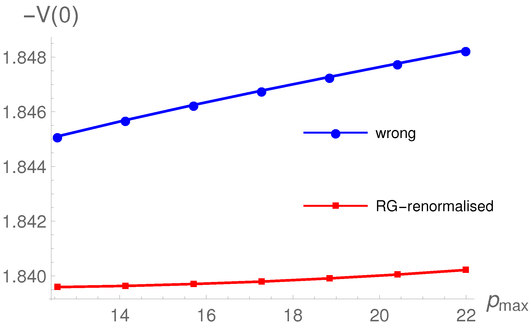
We use points for the integrations over the cosine of the polar angle and the azimuthal angle, and we have checked that all results are stable when we increase the number of grid points in these dimensions. The momentum space grid spacing is where is the spatial lattice spacing and is the number of lattice points for the momentum magnitude. The UV momentum cutoffs are and . We use so that . The numerics are stable if results are unchanged when decreases while is held fixed, and we have checked that this is true if . To test the renormalization we increase while holding fixed. In Figure 1 we show versus . For purposes of comparison we also show a calculation that is done incorrectly, by working at 3 loop level and replacing one of the vertices in the 4 kernel with a bare vertex. We have checked that dependence on the renormalization scale is very small.
To evaluate the 2, 3 and 4 loop approximations in the context of a physical quantity, we calculate the pressure, which can be obtained from the effective action using where V is the 3-volume. To 4 loop order, the contributions to the pressure are
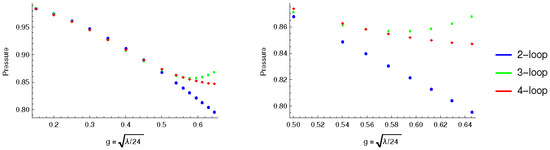
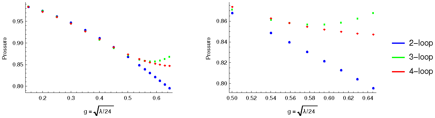
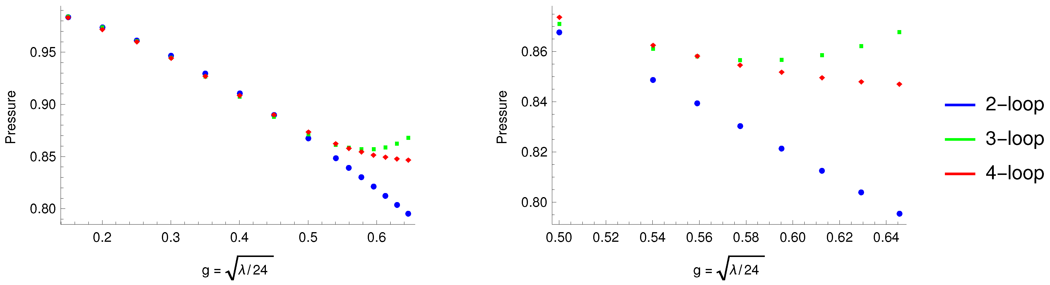
There is a temperature independent divergence that can be subtracted off with a ‘cosmological constant’ renormalization, by setting the vacuum pressure to zero: . The arrow on the right side of (21) indicates that we have dropped a temperature independent constant which would have been removed by this shift. The term is the non-interacting () pressure and since we want to compare to the non-interacting expression, we define . In Figure 2 we show our results for the pressure as a function of the coupling at the 2, 3 and 4 loop orders of approximation.
6. Conclusions
In this paper we present results from a 4 loop 2PI calculation in a symmetric theory with the renormalization done using the RG method of [20]. No counterterms are introduced, and all divergences are absorbed into the bare parameters of the Lagrangian, the structure of which is fixed and independent of the order of the approximation. Our main goal is to use our method to do a calculation with the 4PI effective theory. The basic method is the same, since the form of the flow and Bethe-Salpeter equations are similar [22], but at the 4PI level we must introduce a flow equation for the variational 4 vertex. This calculation is currently in progress.
Author Contributions
Both authors have contributed equally to this work.
Funding
This work has been supported by the Natural Sciences and Engineering Research Council of Canada.
Conflicts of Interest
The authors declare no conflict of interest.
References
- Cornwall, J.M.; Jackiw, R.; Tomboulis, E. Effective action for composite operators. Phys. Rev. D 1974, 10, 2428–2445. [Google Scholar] [CrossRef]
- Norton, R.E.; Cornwall, J.M. On the formalism of relativistic many-body theory. Ann. Phys. 1975, 91, 106. [Google Scholar] [CrossRef]
- Arrizabalaga, A.; Smit, J. Gauge-fixing dependence of Φ-derivable approximations. Phys. Rev. D 2002, 66, 065014. [Google Scholar] [CrossRef]
- Carrington, M.E.; Kunstatter, G.; Zaraket, H. 2PI effective action and gauge invariance problems. Eur. Phys. J. C 2005, 42, 253–259. [Google Scholar] [CrossRef]
- Pilaftsis, A.; Teresi, D. Exact RG invariance and symmetry improved 2PI effective potential. Nucl. Phys. B 2017, 920, 298–318. [Google Scholar] [CrossRef]
- Pilaftsis, A.; Teresi, D. Symmetry-improved 2PI approach to the Goldstone-boson IR problem of the SM effective potential. Nucl. Phys. B 2016, 906, 381–407. [Google Scholar] [CrossRef] [Green Version]
- Markó, G.; Reinosa, U.; Szép, Z. Loss of solution in the symmetry improved Φ-derivable expansion scheme. Nucl. Phys. B 2016, 913, 405–424. [Google Scholar] [CrossRef] [Green Version]
- Markó, G.; Reinosa, U.; Szép, Z. O(N) model within the ϕ-derivable expansion to order λ2: On the existence and UV/IR sensitivity of the solutions to self-consistent equations. Phys. Rev. D 2015, 92, 125035. [Google Scholar] [CrossRef]
- Brown, M.J.; Whittingham, I.B. Soft symmetry improvement of two particle irreducible effective actions. Phys. Rev. D 2017, 95, 025018. [Google Scholar] [CrossRef] [Green Version]
- Van Hees, H.; Knoll, J. Renormalization of self-consistent approximation schemes at finite temperature. II. Applications to the sunset diagram. Phys. Rev. D 2002, 65, 105005. [Google Scholar] [CrossRef]
- Van Hees, H.; Knoll, J. Renormalization in self-consistent approximation schemes at finite temperature: Theory. Phys. Rev. D 2001, 65, 025010. [Google Scholar] [CrossRef]
- Blaizot, J.-P.; Iancu, E.; Reinosa, U. Renormalization of Φ-derivable approximations in scalar field theories. Nucl. Phys. A 2004, 736, 149–200. [Google Scholar] [CrossRef] [Green Version]
- Berges, J.; Borsányi, S.; Reinosa, U.; Serreau, J. Nonperturbative renormalization for 2PI effective action techniques. Ann. Phys. 2005, 320, 344–398. [Google Scholar] [CrossRef] [Green Version]
- Reinosa, U.; Serreau, J. 2PI functional techniques for gauge theories: QED. Ann. Phys. 2010, 325, 969–1017. [Google Scholar] [CrossRef] [Green Version]
- Carrington, M.E.; Kovalchuk, E. Leading order QED electrical conductivity from the three-particle irreducible effective action. Phys. Rev. D 2008, 77, 025015. [Google Scholar] [CrossRef]
- Carrington, M.E.; Kovalchuk, E. Leading order QCD shear viscosity from the three-particle irreducible effective action. Phys. Rev. D 2009, 80, 085013. [Google Scholar] [CrossRef]
- Carrington, M.E.; Fu, W.-J.; Mikula, P.; Pickering, D. Four-point vertices from the 2PI and 4PI effective actions. Phys. Rev. D 2014, 89, 025013. [Google Scholar] [CrossRef]
- Carrington, M.E.; Meggison, B.A.; Pickering, D. 2PI effective action at four loop order in ϕ4 theory. Phys. Rev. D 2016, 94, 025018. [Google Scholar] [CrossRef]
- Carrington, M.E.; Friesen, S.A.; Meggison, B.A.; Phillips, C.D.; Pickering, D.; Sohrabi, K. 2PI effective theory at next-to-leading order using the functional renormalization group. Phys. Rev. D 2018, 97, 036005. [Google Scholar] [CrossRef]
- Carrington, M.E.; Fu, W.-J.; Pickering, D.; Pulver, J.W. Renormalization group methods and the 2PI effective action. Phys. Rev. D 2015, 91, 025003. [Google Scholar] [CrossRef]
- Wetterich, C. Exact evolution equation for the effective potential. Phys. Lett. B 1993, 301, 90–94. [Google Scholar] [CrossRef] [Green Version]
- Carrington, M.E.; Fu, W.-J.; Fugleberg, T.; Pickering, D.; Russell, I. Bethe-Salpeter equations from the 4PI effective action. Phys. Rev. D 2013, 88, 085024. [Google Scholar] [CrossRef]
Figure 1.
The physical vertex versus with , and at 4 loop level in the skeleton expansion. To set the scale we also show the results of an incorrect calculation (see text for more explanation).
Figure 1.
The physical vertex versus with , and at 4 loop level in the skeleton expansion. To set the scale we also show the results of an incorrect calculation (see text for more explanation).

Figure 2.
The pressure as a function of coupling. The right panel shows a close up of the large coupling region where the three approximations start to diverge from each other.
Figure 2.
The pressure as a function of coupling. The right panel shows a close up of the large coupling region where the three approximations start to diverge from each other.

© 2019 by the authors. Licensee MDPI, Basel, Switzerland. This article is an open access article distributed under the terms and conditions of the Creative Commons Attribution (CC BY) license (http://creativecommons.org/licenses/by/4.0/).
Share and Cite
MDPI and ACS Style
Carrington, M.E.; Phillips, C.D. Four Loop Scalar ϕ4 Theory Using the Functional Renormalization Group. Universe 2019, 5, 9. https://0-doi-org.brum.beds.ac.uk/10.3390/universe5010009
AMA Style
Carrington ME, Phillips CD. Four Loop Scalar ϕ4 Theory Using the Functional Renormalization Group. Universe. 2019; 5(1):9. https://0-doi-org.brum.beds.ac.uk/10.3390/universe5010009
Chicago/Turabian StyleCarrington, Margaret E., and Christopher D. Phillips. 2019. "Four Loop Scalar ϕ4 Theory Using the Functional Renormalization Group" Universe 5, no. 1: 9. https://0-doi-org.brum.beds.ac.uk/10.3390/universe5010009
Note that from the first issue of 2016, this journal uses article numbers instead of page numbers. See further details here.