Simultaneity and Precise Time in Rotation


Defence Science and Technology Group, CEWD 205 Labs, P.O. Box 1500, Edinburgh SA 5111, Australia
Universe 2019, 5(12), 226; https://0-doi-org.brum.beds.ac.uk/10.3390/universe5120226
Submission received: 4 October 2019
/
Revised: 11 November 2019
/
Accepted: 12 November 2019
/
Published: 16 December 2019
(This article belongs to the Special Issue Rotation Effects in Relativity)
Abstract
:I analyse the role of simultaneity in relativistic rotation by building incrementally on its role in simpler scenarios. Historically, rotation has been analysed in dimensions; but my stance is that a -dimensional treatment is necessary. This treatment requires a discussion of what constitutes a frame, how coordinate choices differ from frame choices, and how poor coordinates can be misleading. I determine how precisely we are able to define a meaningful time coordinate on a gravity-free rotating Earth, and discuss complications due to gravity on our real Earth. I end with a critique of several statements made in relativistic precision-timing literature, that I maintain contradict the tenets of relativity. Those statements tend to be made in the context of satellite-based navigation; but they are independent of that technology, and hence are not validated by its success. I suggest that if relativistic precision-timing adheres to such analyses, our civilian timing is likely to suffer in the near future as clocks become ever more precise.
Keywords:
rotating disk; clock synchronisation; precise timing; Sagnac effect; accelerated frame; circular twin paradox; Selleri’s paradoxPACS:
03.30.+pMSC:
83A051. Introduction
The analysis of relativistic rotation has evolved from a theoretical problem to a practical one in recent years as clock technology has grown ever more precise, and the question of what constitutes “the best time” on a rotating Earth becomes more urgent to resolve. The quest for insight into how the world appears to an observer at rest on a rotating disk goes back to the earliest days of relativity. Numerous analyses have appeared in the literature [1], but—unlike studies of constant-velocity observers—no single analysis of rotation is agreed upon by the relativity community. Special relativity is traditionally taught using one space dimension (and of course one time dimension, hence “ dimensions”), with little room generally reserved for discussion of two or three spatial dimensions. Perhaps this is the reason that the rotating disk has always been described using a formalism, even though the disk rotates in two spatial dimensions.
The stance that I take in this paper is that analyses of the disk are not just insufficient, but inherently faulty. This view should not be considered contentious; after all, even a non-relativistic discussion of, say, the Coriolis force on a rotating disk in any classical mechanics book accepts it as obvious that the scenario requires two space dimensions. No one chains together a continuum of constant-velocity one-dimensional frames in such analyses. Why, then, should it be assumed that a continuous chain of Lorentz transforms must describe the relativistic disk?
Much, even most, discussion of the rotating disk has sought to predict the physical changes undergone by the disk as it is spun up, due to the stresses incurred in the process. I believe this dynamical analysis to have been an early distraction in the study of relativistic rotation that only shunted the subject onto a disused side track that went nowhere. Relativity is firstly a kinematical theory, and no analysis of stresses and strains is traditionally performed for the straight-line acceleration necessary to create the constant-velocity “primed frame” in derivations of the Lorentz transform. This inertial primed frame that moves in the unprimed laboratory frame (the laboratory will always be taken as inertial in this paper) is always treated as having been moving at constant velocity forever. Likewise, although in this paper we certainly describe how the disk can be spun up, we will quickly take the procedure as a given, and will effectively always treat the disk as having been spinning forever with a fixed angular velocity.
Ehrenfest [2] referred to attempting to spin the disk up from rest in the lab in a “Born-rigid” way, meaning the disk remains rigid from the viewpoint of observers riding on it. Thus, an attempt is made to spin the disk such that each element of it Lorentz contracts in that element’s direction of motion in the lab, so that an observer fixed to that element states that the element retains its original length. It is well known that Born rigidity is incompatible with a spinning disk. In contrast, the simplest spin possible is to arrange for all points on the disk to be equally rotated in the lab, at any moment, from their positions at any other moment. They have helical world lines when drawn in the inertial lab’s spacetime, such that points that are designed to lie on radial lines in the lab remain radial, and all helices of any particular radius are congruent in the lab’s spacetime. I will discuss and always use this sense of rotation in this paper. It is “laboratory rigidity”: the disk’s molecules are guided so that the disk remains rigid in the lab as it is spun up.
An early point of language must be made: I use the equivalent phrases “I observe” and “I measure” to mean constructing a history of events based on data supplied by other observers in my frame, who each have the sole job of recording only the events that occur in their close vicinity. In contrast, “I see” denotes building a picture of events based on my recording the arrival of light rays from them. In this paper I concentrate exclusively on what is observed, not what is seen.
To establish how observations might be made by an observer at rest on the spinning disk, in 1935 Langevin [3] expressed (primed) polar coordinates of an observer riding on the disk that spins with angular velocity in the inertial lab in terms of (unprimed) lab coordinates, by using a rotational Galilei transform:
Although this is a valid one-to-one coordinate map, such a Galilei transform need have no physical relevance to a rotating disk, as had already been stated by Franklin in 1922 [4]. Likewise, we will not assume that a Galilei transform has any physical relevance to the relativistic disk—kinematic or dynamic. Also, the use of general relativity (curved spacetime) is not appropriate here, because the disk is simply a collection of helical world lines in a flat spacetime, and a spacetime that is flat for one observer is flat for all observers.
Section 3, Section 4.3, and other parts of this paper are taken from my analysis in [5]. Section 5 streamlines some of my analysis of the rotating disk in [6]. Refer to these publications for further details.
2. The Generalised Pole and Barn Paradox
Our first step in studying the accelerated motion of a rotating disk involves a variant of the classic “pole and barn paradox”. The standard paradox involves a runner carrying a pole at relativistic speed toward a small barn. The pole’s rest length is greater than the barn’s rest length, but being Lorentz contracted, the pole easily fits inside the barn. But in the runner’s frame, the barn is Lorentz contracted and can never contain the pole. Various versions of the paradox have the barn’s front and back doors being opened, or not, to either allow the runner to pass through the barn unscathed, or to crash into the back door. All are well explained by noting that the runner’s standard of simultaneity differs from that of the barn. (Probably all of special relativity’s paradoxes are resolved by examining the different standards of simultaneity of all participants; time dilation and length contraction usually play only a minor role.)
In our variant of this paradox, suppose that the runner’s motion has been pre-arranged by us using tiny rockets, with one rocket attached to each atom (so to speak) of the runner and pole. We have programmed these rockets to produce the following scenario. The runner carries the pole at relativistic speed into the barn. The rockets have acted on each atom to contract the pole along its length in whatever way we choose; as long as it fits in the barn. It is then carried in circles (with its velocity vector always parallel to its length) for an arbitrarily long period with the barn sealed. After some time the barn door opens and the runner and pole exit, with never any contact had with the walls. This scenario is perfectly valid, and yet it’s clear that the runner cannot perform any traditional “Lorentz-contracted barn” analysis of what has taken place. Hence we cannot state a priori that “moving objects are Lorentz contracted” here, since that would clash with the runner’s experience inside the closed barn. Apparently, the runner’s view of events is not simple. To proceed, we must carefully define a frame.
3. Definition of a Frame, and Simultaneity
A reference frame, or simply “frame”, is a set of observers who obey the following requirements:
- All of the observers in the set measure their displacements from all of the other observers in the set to be fixed: this means they form a rigid lattice, enabling them to agree on the construction of a single set of space coordinates. Their fixed separation defines their common unit of distance.
- All events measured as simultaneous by any chosen observer in the set are measured to be simultaneous by all of the observers in the set. Hence the observers can agree on the use of a single time coordinate: they have a common clock. This time coordinate can be the proper time of one of the observers (the “master observer”), but it need not equal the proper times of the other observers. The fact that the observers might all be ageing at different rates is immaterial; each observer can gear his clock appropriately so that all clocks tick at the same rate. Hence, all observers will agree that all clocks display any given time simultaneously for all of them.
Each observer occupies a fixed point on the lattice and holds his own clock. He records the positions and times of events only in his immediate vicinity. All the observers continuously send these “time-and-space”-stamped recordings to a master observer, who continuously collates this information to form a global picture of all events in spacetime. This procedure does away with the master observer having to make direct observations of events himself, for which he would require to know the time of travel of the signal coming from each event to him. Nonetheless, we can refer to this procedure as the master observer “observing an event”. It’s normal to use the words “observer” and “clock” as synonyms, and so we will use “clock” when it simplifies the language in the descriptions that follow. Note that in discussions of inertial frames, “observer” is often taken as synonymous with “frame”. This is fine as it stands, but we will make a minor distinction when considering non-inertial motion, since the kinematics of the observers then being studied need not be identical when measured by an inertial frame.
The above two requirements for the existence of a frame certainly hold for inertial frames in special relativity. Crucially, they also hold for the well-known “uniformly accelerated frame” discussed in Section 3.2. Both of these frames have a global standard of simultaneity. For observers with other kinematics, some analysts alter this global standard to become a local standard. That is, they define simultaneity for each observer only locally to that observer; then, in -D, they attempt to join neighbouring infinitesimal line segments of simultaneity into a single curve. In -D, they join neighbouring infinitesimal surfaces of simultaneity into a single global surface. Yes, this procedure does recreate the global standard of simultaneity for inertial and uniformly accelerated frames. But more generally it fails, because (a) it implies that the determination of the events that are simultaneous for one observer is altered by the state of motion of his neighbours; and (b) it assumes, incorrectly, that simultaneity across differently moving observers is transitive. Basic special relativity tells us that simultaneity is not transitive: two observers with different constant velocities inhabit different frames, and they simply disagree on simultaneity. Note too, that if the observers are fixed to a rotating disk, then any such stitched-together surface of simultaneity becomes a screw spiraling around the world line of the centre of rotation, forcing each observer to conclude that his present is simultaneous with events in his causal future and past. We conclude that this stitching-together procedure is invalid. So, we will demand the existence of a global simultaneity shared by all observers who make up a frame; else there is no frame. See my further comments on this near the end of Section 3.2.
Non-relativistic frames obey the above two conditions only up to some approximation. One approximately globally inertial frame is that of the distant stars but “in Earth’s vicinity”, in which Earth turns once per sidereal day. This is conventionally called the “Earth-centred inertial frame” (ECI)—actually a misnomer, because inertial frames do not have centres. Another commonly used frame is the “Earth-centred Earth-fixed frame” (ECEF), which is the everyday civilian world of our Earth, in which Earth does not turn, and in which the celestial sphere rotates around us once per sidereal day. We’ll see shortly that the ECEF fails the second condition above to a small extent, special-relativistically speaking, because its observers cannot agree on simultaneity to a high accuracy; but, for convenience, we still call it a frame.
Special relativity’s definition of simultaneity accords with what we require of frames: it defines two events to be simultaneous if two signals of equal speeds that were sent from halfway between the sites of those events will intercept the events. In principle in an inertial frame, the synchronisation can use any type of signal, provided its speed characteristics are well known: even sound, or two rubber balls. We (along with everyone else) use light rays for two reasons. First, since inertial frames are assumed to admit no privileged directions, light’s speed can be taken as independent of its direction of travel in those frames, and independent of any bounce it undergoes. Second, because all observers agree on light’s speed, we can draw all light rays emitted by a moving observer as if those rays had been emitted by a fixed observer. This cannot be said of sound or rubber balls, and it makes the analysis particularly easy when light rays are used.
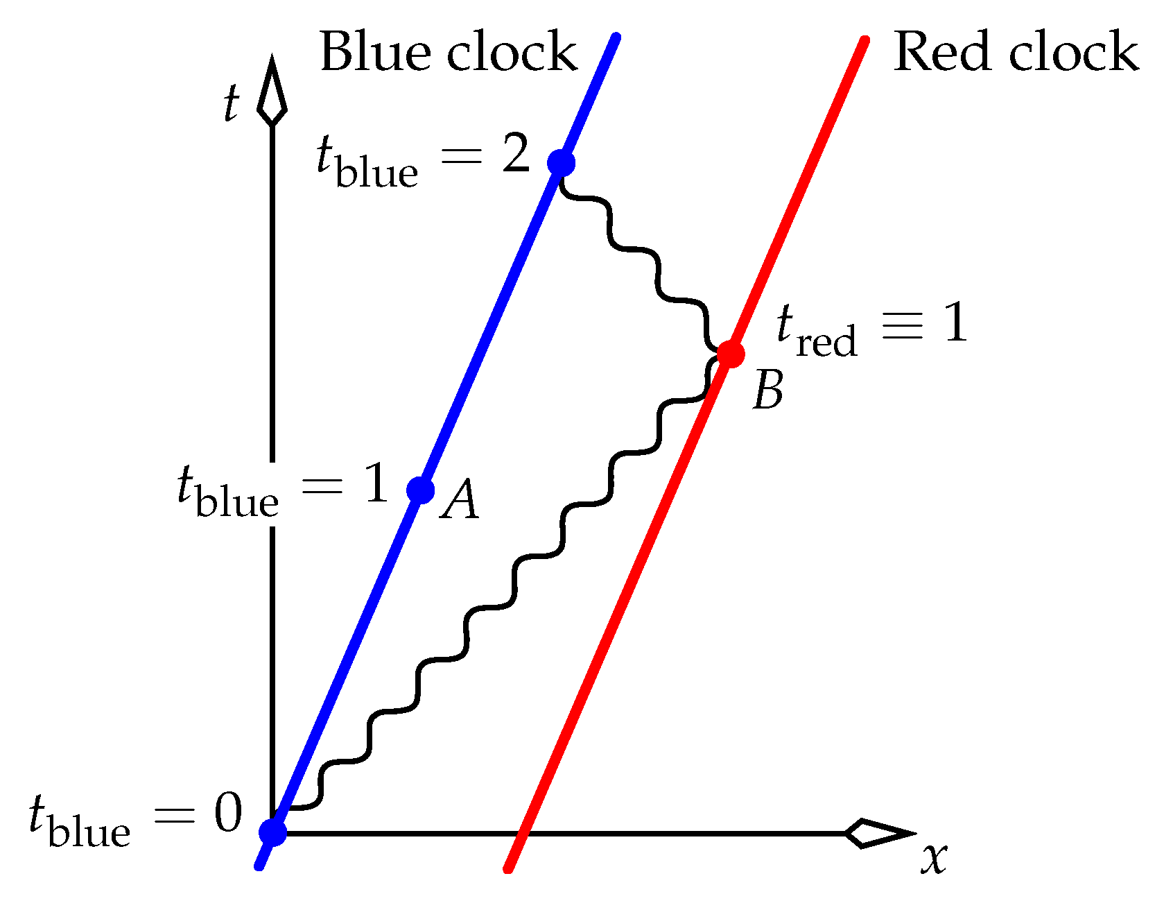
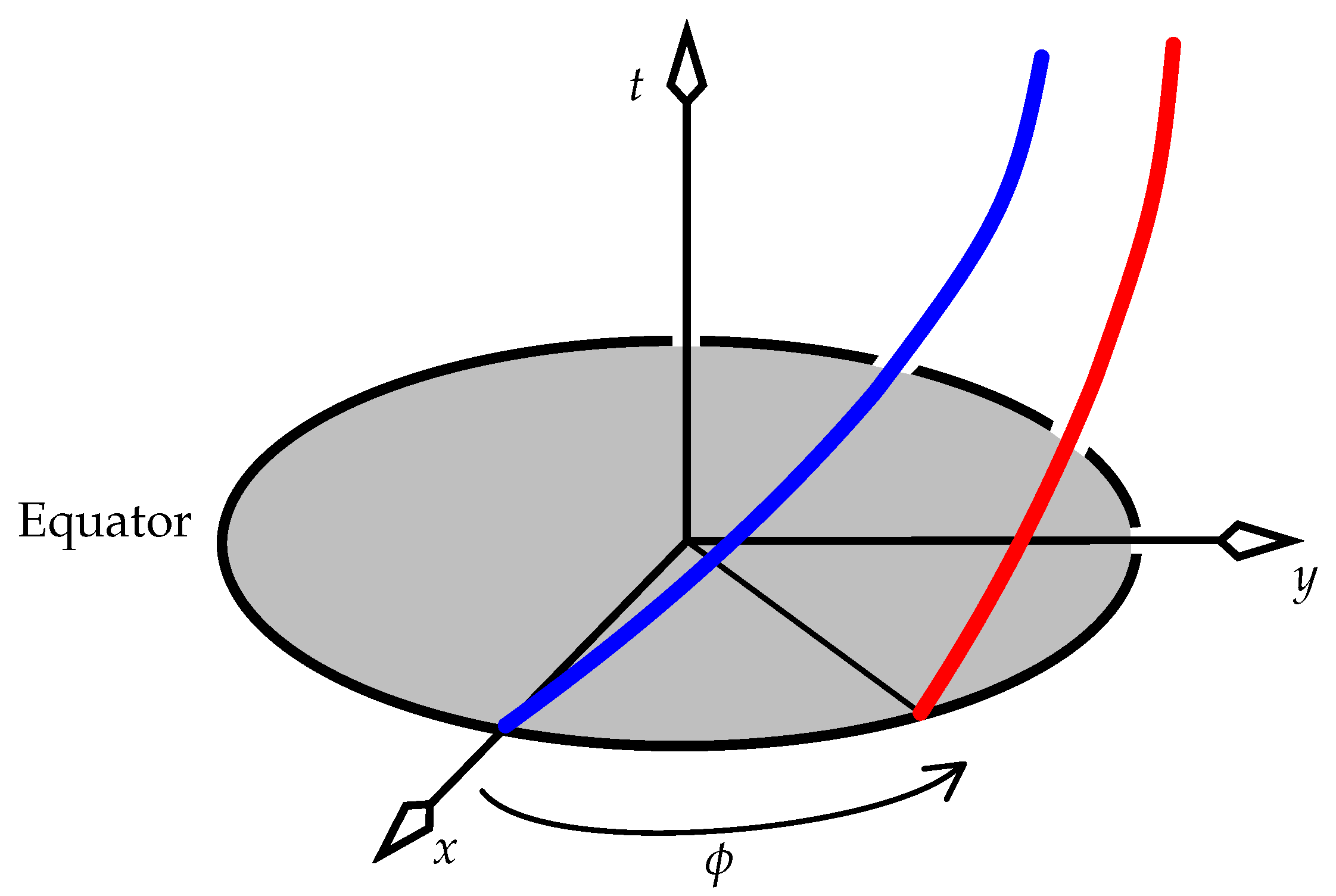
The postulated invariance of all inertial frames dictates that we can synchronise a distant clock of our frame with our own clock by sending the distant clock a signal that sets its display to be our current display plus the trip time of the signal.1 Figure 1 shows this procedure being performed in an inertial frame (the rest frame of the blue and red clocks) that moves at constant velocity in the inertial laboratory frame described by the black axes. As mentioned in the previous paragraph, we can draw the light ray emitted by the moving blue clock and the ray bounced from the red clock as if they had been emitted and bounced from observers at rest in the lab. Thus, we draw them at , so that light has speed 1 in the figure.
The blue clock wishes to synchronise the red clock with itself. Blue’s signal is bounced from Red in what is a “radar measurement” of the distance between the clocks. Blue receives the return after 2 seconds, and infers that the one-way travel time must have been 1 second. With that prior knowledge, because Blue sent the signal out when its clock displayed zero, it arranged beforehand for Red to display 1 second when the signal reached Red. (Of course, in practice this procedure requires two pulses and no relative motion between Blue and Red: the first signal determines the distance, and the second does the synchronising. We have combined both signals into one for brevity.)
It’s immediately clear that in the laboratory frame (which has the black axes in Figure 1), the two events A and B occur at different lab times. When we fill the space with a continuum of clocks that all share the same velocity in the lab, all events on the line containing A and B will be defined by all the moving clocks to be simultaneous with A and B, for the case of one spatial dimension in Figure 1. This line of events is the “line of simultaneity” at any event on that line for the frame of the moving clocks. If we augment Figure 1 with another space dimension (a y axis normal to the page), all events simultaneous with A and B will lie on a plane of simultaneity, whose normal lies in the plane of the page.
The procedure of synchronising clocks with constant and equal velocities in Figure 1 is sometimes called “Einstein synchronisation”. History aside, I think this label is misleading, because some misinterpret it to imply that the very definition of synchronisation was an arbitrary choice made by Einstein, and hence is something that can be changed on the fly to suit our tastes or to get us out of a perceived bind—as occurs in [7], whose author simply states that simultaneity’s definition is arbitrary, without giving a supporting argument. But Einstein’s “choice” was not arbitrary. He had only one choice in how to synchronise, because his method is a natural by-product of a deep and fundamental tenet of all of physics: that all inertial frames share an equal footing. It is imposed on us by physics, and we do not get to change it at our whim.
Given a frame, a coordinate system can be created by numbering the lattice points with distances from an origin, and times since some epoch. We are free to use any coordinate system; a given coordinate system need not have any relationship to a given frame. But although frames and coordinates are not related, a choice of frame may well suggest some natural choice of coordinates. The most natural time coordinate labels with the same number all events that are simultaneous; indeed, this is precisely why the Lorentz transform exists. Although we can always write a Galilei transform of coordinates in a relativistic context because it is just a one-to-one map of numbers, the coordinates that result will not behave in the way that we expect and require good coordinates to behave. In particular, two events that are simultaneous (such as A and B in Figure 1) will not necessarily have the same Galilei time coordinate; and two events with the same Galilei time coordinate will not necessarily be simultaneous. This makes the Galilei time coordinate generally useless to describe a set of events. For example, ordering the events in a discussion about causality will be difficult when this coordinate is used.
Although we are always free to use the coordinates from one frame (say, the ECI) to describe events in another (say, the ECEF), we must always be aware that when doing so, we can no longer interpret equal time coordinates natural to one frame as denoting events that are simultaneous in another frame. This requirement to describe simultaneity that a good time coordinate must obey appears not to be well understood in the modern field of precise timing. There, practitioners tend to insist that because relativity can be expressed in tensor language, then any choice of coordinates is as good as any other. Examples are [8,9], which use a Galilei transform in a relativistic context.2 Section 2.4 of [10] makes no distinction between arbitrary coordinate choices and the real physics of relativity, which is built on establishing simultaneity and defining frames, and says incorrectly that simultaneity is defined by coordinates. To say or imply that all coordinates are as physical as any other is akin to saying that a Galilei transform is sufficient in modern physics, with the Lorentz transform being just a distraction: clearly, incorrect. Tensors are certainly useful for writing equations in a form that doesn’t single out a particular choice of coordinates; but this does not imply that any choice of coordinates is as physically meaningful as any other—and hence, it does not imply that a given choice of coordinates has anything to do with a given frame, or that it even defines a true relativistic frame at all.
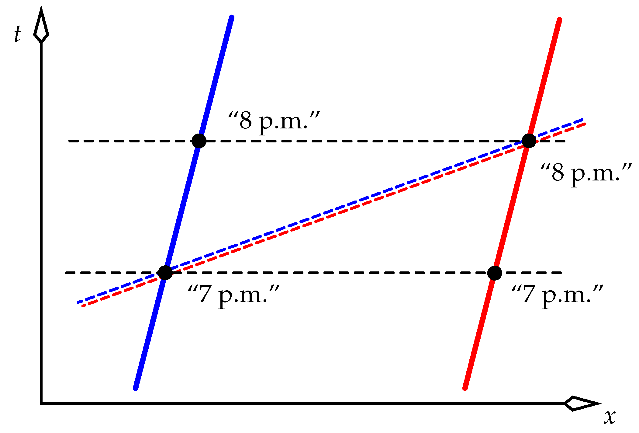
What if the clocks in an inertial frame that moves in the lab have been synchronised in the lab, as shown in Figure 2? There is no problem here. Observers Blue and Red certainly agree on the simultaneity of all events, and displays on clock faces have no bearing on that. At the lower-left event marked with a black dot, Blue displays 7 p.m. At this event, Blue’s line of simultaneity is the blue dashed line. Blue says “When I display 7 p.m., Red displays 8 p.m.” Red’s line of simultaneity (red dashed) at Red’s 8 p.m. coincides with Blue’s line of simultaneity at Blue’s 7 p.m. Red says “When I display 8 p.m., Blue displays 7 p.m.” Blue and Red thus share a common standard (a line) of simultaneity, and can be shown each to measure the other to be at a fixed distance. Hence, they define a frame. Because they do, they are free to set Red’s display back by one hour, so that they both assign all simultaneous events the same time coordinate. That is a reasonable thing to do, of course, because it gives the now common coordinate time of Red and Blue physical significance and utility.
The above procedures are all well defined and well known. But despite the best efforts of textbook authors, the statement can still be found on any number of web sites (and also on the fringes of physics) that two events are defined to be simultaneous by a single observer if they are merely seen at the same time, even though they occurred at different distances from the observer. This is a trivial misunderstanding of simultaneity; compare it with the correct definition, which concerns when events occur: all times of travel of signals from those events to an observer are assumed known to the observer, who then subtracts those travel times from the current time to find the signals’ times of emission. (Or equivalently, the “master observer” doesn’t know the signal-travel times, but employs a continuum of observers throughout space who each record only what happens in their immediate vicinity and report back to the master observer.) This misunderstanding of simultaneity should have no place in journal papers or magazine articles, and yet it continues to appear even there. For example, references [11,12] both apply a lack of understanding of basic simultaneity to conclude that relativity itself is incorrect. What appears to be an incorrect definition based only on what is seen even appeared some years ago in the Encyclopedia Britannica.3
3.1. Identically Accelerated Observers and the MCIF
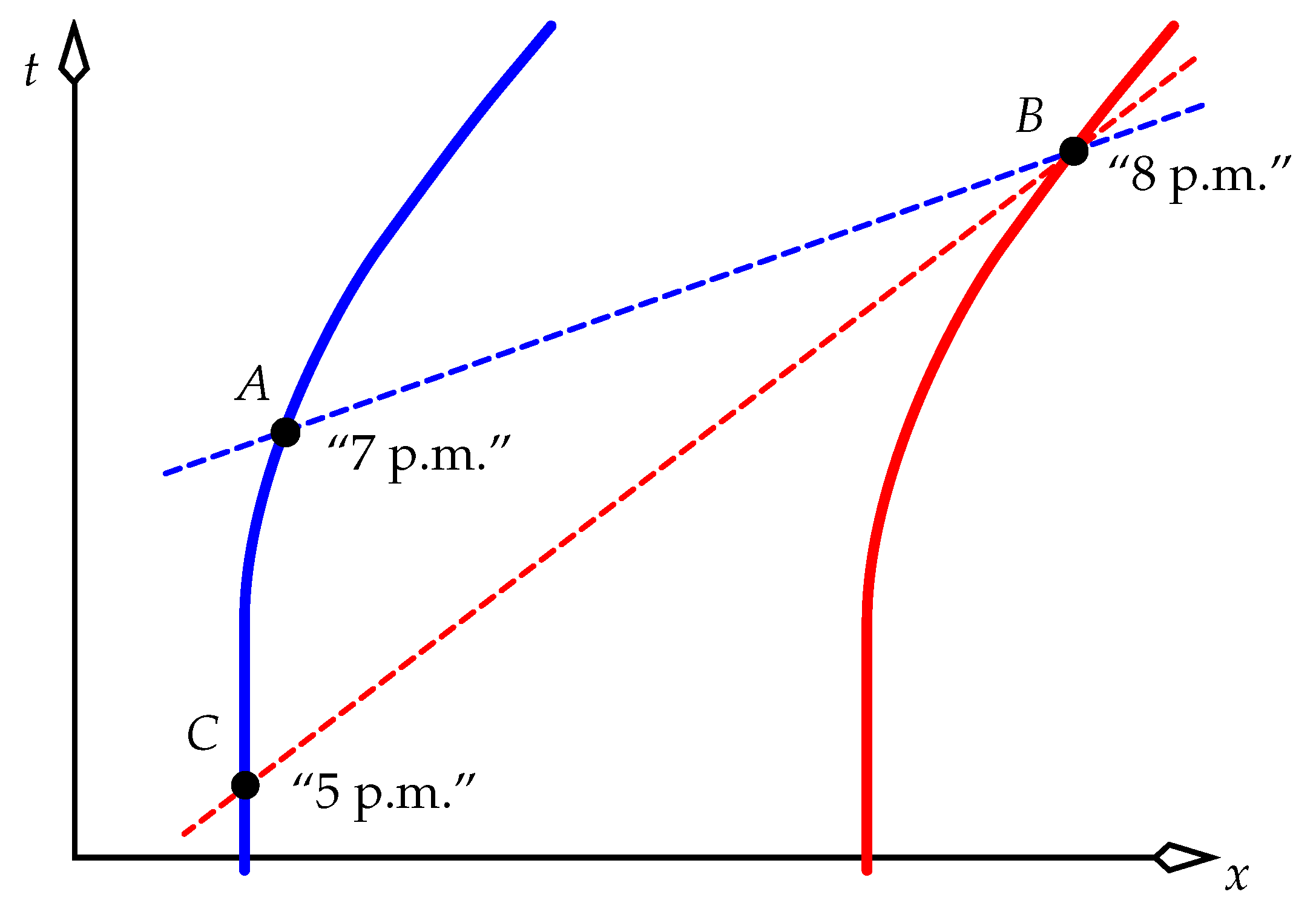
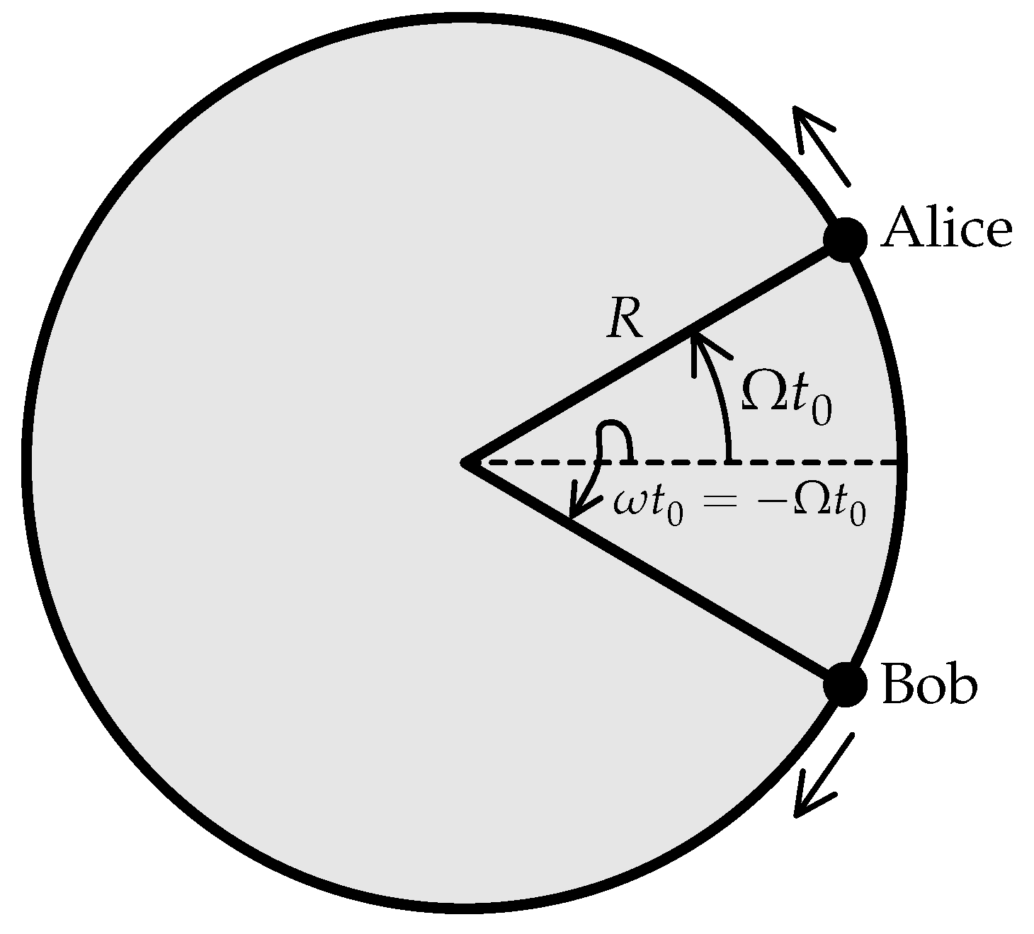
The next level of complexity beyond inertial observers involves two identically accelerated observers, shown in Figure 3. Do they agree on the simultaneity of events? Simultaneity in relativity is most naturally defined for inertial observers, for whom we can make well-understood statements about the speed of signals such as light. Relativity postulates that local measurements made by a non-inertial observer are always identical to measurements of the same events that are made in his “momentarily comoving inertial frame” (MCIF): at a given event, this is the inertial frame that is momentarily at rest relative to the non-inertial observer. The MCIF is thus the frame of an inertial observer whose world line is tangential to the accelerated observer’s world line at the event of interest [13].4 So, from moment to moment, the accelerated observer occupies a succession of MCIFs. We’ll see in Section 3.2 that this postulate of using MCIFs has a modern experimental underpinning.
When analysing the standard examples of straight-line motion in relativity textbooks, it is usually sufficient to examine lines of simultaneity for all observers, who usually have constant velocity. For accelerated motion, we examine lines of simultaneity of all relevant MCIFs. That is, we draw the line of simultaneity at each event on a world line by using only the tangent to the world line at that event. This line of simultaneity generally changes from event to event.
For example, consider the two identically accelerated observers in Figure 3, who have clocks that have been synchronised not by them, but in the inertial lab frame of the picture: at any moment, the lab says that Blue and Red display the same time. At event A, Blue displays 7 p.m. and says (via the blue dashed line of simultaneity at A, belonging to the MCIF at this event) “When I display 7 p.m., Red displays 8 p.m. at event B”. At B we draw the red dashed line of simultaneity for Red, and note that this has a different slope to the blue dashed line, because Red’s MCIF at B has a faster speed in the lab than Blue’s MCIF at A. Red thus says (via the red dashed line of simultaneity at B) “When I display 8 p.m., Blue displays 5 p.m. at event C”. These observers do not share a common standard of simultaneity: they don’t have a “shared now”. Also, it can shown that they don’t each measure the other to maintain a fixed distance. Hence they do not form a frame.
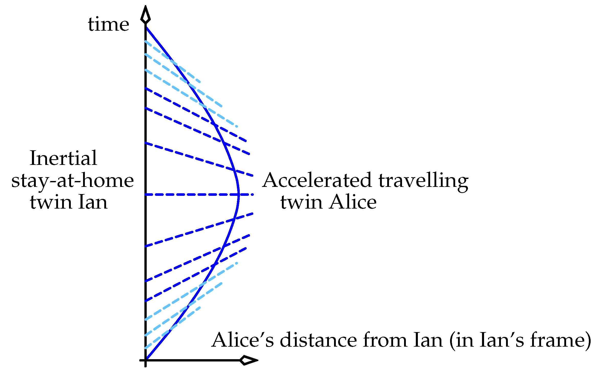
Another example of the use of MCIFs is the analysis of the well-known twin paradox, shown in Figure 4. The figure is drawn in the frame of the inertial stay-at-home twin Ian. The travelling twin, Alice, starts with some velocity to the right in the figure, and always accelerates to the left.
Inertial Ian’s description of accelerated Alice’s ageing can be formed by examining Ian’s horizontal lines of simultaneity (not shown) at a succession of events spread evenly in time. Ian’s line of simultaneity simply translates through spacetime, and so he always observes Alice to age slower than himself.5
Alice’s description of Ian’s ageing is formed in the same way, by drawing Alice’s dashed line of simultaneity through a sample of events on her curved world line in the figure (as shown). When the twins are close together, Alice observes Ian to age slowly, because her line of simultaneity mostly translates through spacetime (successive snapshots of this line are drawn in light blue). Near their greatest separation, Alice observes Ian to be ageing quickly, because her line of simultaneity now rotates through spacetime (successive lines are drawn in dark blue). Finally, as Alice nears home, her line of simultaneity again mostly translates through spacetime (drawn light blue), and she again observes Ian to age slowly. (Be reminded that we are not discussing what Alice and Ian see here, as per my comment in Section 1.) Alice concludes that when she is accelerated, the common phrase “moving clocks tick/age slowly” applies only to clocks in her vicinity. Distant clocks can age at other rates.
Many versions of the paradox give Alice constant-velocity outbound and inbound flights, joined by a moment of infinite acceleration at her turn-around point. These are easier to analyse than the above discussion because they don’t require mention of MCIFs; but they are far less illuminating, because they make Alice’s line of simultaneity jump discontinuously through spacetime at her turn-around point. This discontinuous jump is as non-physical as her infinite acceleration, and its effect is only to hide the period in which Alice maintains that Ian is ageing quickly. Thus, a crucial part of the explanation of the paradox is sacrificed to simplicity. Simplifying the paradox’s scenario to two constant-velocity legs in this ways ends up throwing the baby out with the bath water.
3.2. The Uniformly Accelerated Frame
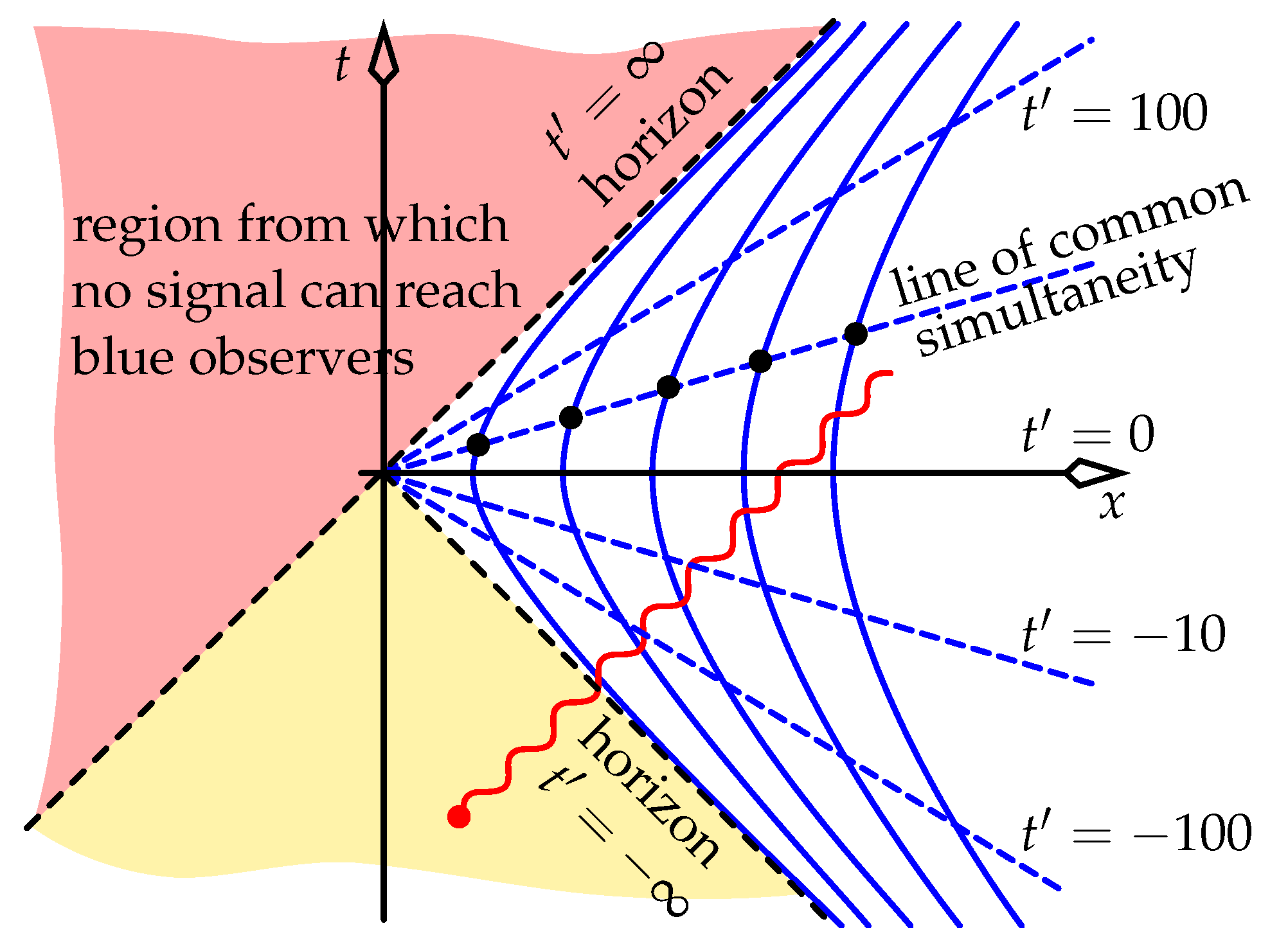
Suppose that a set of observers is accelerated in a fixed direction in an inertial frame. Each observer’s proper acceleration is constant and proportional to the reciprocal of that observer’s distance from an origin at the moment that they all have zero velocity. A set of these observers appears in Figure 5. Their solid-blue world lines can be shown to be hyperbolae: see Chapter 7 of [14]. These observers turn out to constitute a frame, called the “uniformly accelerated frame” (also known as Rindler space), because each observer physically feels a constant acceleration forever: the acceleration of each observer in his MCIF is a constant for all time. (This does not mean that each observer accelerates at a constant rate indefinitely; a uniformly accelerated observer’s speed asymptotes to the speed of light. Also, remember that the acceleration felt by an observer depends on his distance from the origin.)
Details of how this uniformly accelerated frame is constructed using the MCIF at each event are given in [14,15], but the important point is that it is constructed from MCIFs. All of the accelerated observers will measure the distance between any pair of observers to be constant for all time. Also, each intersection of a solid blue world line (a hyperbola) and a dashed blue straight line is an event whose co-located observer’s line of simultaneity is precisely that dashed line. Thus, all observers agree that all events on any given dashed line (say, the black dots in Figure 5) occur at the same moment. These two facts of distance and time mean that the set of uniformly accelerated observers is indeed a frame. The events that they all agree are happening “now” can be allocated a single time coordinate: say, the proper time of a particular chosen “master” observer, who can be any of the observers. The observers’ clocks, if manufactured identically, will age (and thus tick) at different rates; but these clocks can be geared in such a way that they tick at the same rate. In that way, all observers can always say “When my clock displays 7 p.m., all other observers’ clocks display 7 p.m., even though I don’t see their clocks displaying this time right now, because it takes some time for their light to reach me.” The blue hyperbolae in Figure 5 define curves of constant (the accelerated frame’s space coordinate), and the dashed lines define events of constant , the frame’s time coordinate. The event at the origin of the figure’s axes is simultaneous with all events in the accelerated frame. In that frame, time at this event has slowed to a stop; and to this event’s left (), time runs backwards.
Uniformly accelerated observers call the events of the black dashed line bordering the red region in Figure 5 a “horizon”, because no signals from that red region (from “below the horizon”) can reach them. Like the red region, left-moving signals from the yellow region cannot reach the observers. But right-moving signals from the yellow region—such as the red light coming from the red event—will be seen by the observers; and yet the red event is not simultaneous with any event on any blue line. So the uniformly accelerated frame can see this red event, but cannot ascribe a time to it: no number in the interval to ∞ can be allocated to that event.
Requirement 2 in Section 3 distinguishes between the rate of a clock’s ageing (its proper time) and the rate of its ticking (its display: coordinate time). At any given moment in the inertial lab frame, uniformly accelerated observers who are farther from the origin (“higher up/farther from the horizon”) are moving more slowly in the lab (and hence age faster) than those who are “lower down”. Hence, these higher-up observers must gear their clocks’ tick rates down more strongly the farther they are from the origin.
For an example of observers who share a common simultaneity, consider two such who have lived their whole lives in a uniformly accelerated rocket, and who agree that they were born simultaneously. Observer “Engine” is lower down, near the engine, and Observer “Nose Cone” is higher up, near the nose cone. Engine says “At the moment I was born, Nose Cone was born”, and Nose Cone says “At the moment I was born, Engine was born”. Later, Engine says “When I was a 1-year-old baby, Nose Cone was an old man, aged 100 years”. Nose Cone says “When I was an old man, aged 100 years, Engine was a 1-year-old baby”. For general motion where observers don’t share a common simultaneity, Nose Cone’s statement above need not follow from or be equivalent to Engine’s statement, in the same way that Figure 3’s blue and red observers don’t share a common simultaneity. In that figure, Blue might say “When I was a 1-year-old baby, Red was an old man, aged 100 years”, whereas Red might say “When I was an old man, aged 100 years, Blue was not yet born”. There, Blue and Red don’t constitute a single frame.
In the uniformly accelerated frame where Nose Cone ages 100 times as fast as Engine, Nose Cone’s clock can be geared down by a factor of 100. Then both will agree that their clocks display any nominated value simultaneously for each.
Such gearing of clocks in the accelerated frame creates a time coordinate that obeys the equivalence principle of general relativity. That is, if we compare a clock’s displayed time with its age (its proper time ) throughout the interior of a small rocket (by calculating ), we get a result that agrees to high precision with the corresponding comparison for the Schwarzschild metric in a region of small extent in real gravity, as shown in Chapter 12 of [14]. For example, clocks in the orbiting satellites of the Global Positioning System (GPS) age slightly quicker than they do on Earth, and so are manufactured to “tick” slightly slowly on Earth before being sent into orbit. Hence, when they arrive in orbit, they tick at the same rate as Earth clocks. They display an ECI coordinate time that is used in all GPS calculations. This is a real example from technology of the distinction between proper time (their ageing) and coordinate time (their ticking). The uniformly accelerated frame with its “pseudo gravity” thus becomes the stepping stone, via Einstein’s equivalence principle, to a consideration of clock rates in real gravity. The success of GPS in a curved spacetime and classic experiments such as that performed by Pound, Rebka, and Snider can be taken as experimental validation of the technique of building a flat-spacetime uniformly accelerated frame from MCIFs.
It should be noted that although the uniformly accelerated frame is constructed from knowledge of the MCIF at each event on each accelerated observer’s world line, this does not imply that any frame is just a union of MCIFs, to be analysed without regard for the gearing of clocks that is necessary to create a global time coordinate. Hence, at any moment, an accelerated observer’s measurements of distant events generally differ from measurements made by his MCIF at that moment.
It’s clear here that simultaneity plays a major role in the uniformly accelerated frame, and we are not at liberty to redefine it at our whim. In contrast, many precise-timing practitioners, and some physicists, believe that simultaneity can be redefined in whatever way one chooses [16]. I maintain that the belief that simultaneity is arbitrary renders it meaningless, and also that such arbitrariness contradicts the tenets of relativity at a most basic and obvious level. If we allow an arbitrary definition even within the simplicity of an inertial frame, then we essentially create a set of meaningless and mutually contradictory statements that are of no use to anyone.
Why is the belief so widespread that simultaneity is arbitrary, given my argument above about its experimental validation in GPS? My argument rests on a knowledge of the uniformly accelerated frame. This frame is sometimes introduced using arcane mathematics in dusty corners of a few books on relativity. But, surprisingly, any real discussion of its full worth—as a flat-spacetime approximation to the frame of a real laboratory on Earth—is almost absent from relativity courses and textbooks.6 The equivalence principle links the pseudo gravity of an accelerated frame to a discussion of real gravity in relativity. Referring to Pais’s biography of Einstein [17], it seems that when Einstein first discussed acceleration in relativity, his aim was to make an immediate link to gravity. Modern writers have followed suit, using only very short discussions of acceleration to segue quickly into a discussion of gravity proper. I think that such abbreviated analyses bypass the richness and subtlety of uniformly accelerated motion as a subject in its own right that can shed light on other areas of relativity [14].
The use of the uniformly accelerated frame is related to the question of whether it makes sense to draw lines of simultaneity arbitrarily far from an accelerated observer’s current position. A few commentators, such as [18], believe that Alice’s lines of simultaneity in Figure 4 cannot be extended very far from her at each moment, since doing so will make them see-saw wildly if Alice decides to walk forwards and backwards. But firstly, this see-sawing creates no logical or experimental contradictions. It can create a problem of defining coordinates if the lines are extended so far that they intersect; but that is less about the physics than about choices of coordinates. (Consider that problems of defining coordinates are well known in relativity, such as with Schwarzschild coordinates at the horizon of a black hole; but such problems certainly don’t negate the theory of black holes.7) Second and more importantly, forbidding Alice’s lines of simultaneity to extend arbitrarily far from her has a show-stopping consequence: it destroys our ability to consider, say, just two uniformly accelerated observers who are far apart, since then their short lines of simultaneity are too far apart to “link arms”, and so we cannot discuss how they observe the world. And yet we should be able to discuss how these observers relate to each other. Rather, by allowing their lines of simultaneity to extend arbitrarily far so that these lines are clearly seen to be the same line, allows us to call on the uniformly accelerated frame’s quantitative prediction that clocks high “above” us in that frame will run faster than ours [14]; we can then combine that idea with Einstein’s equivalence principle to segue into a correct quantitative prediction that clocks high above us in a real gravity field will run faster than ours. In other words, forbidding lines of simultaneity to extend arbitrarily far prevents us from discussing the equivalence principle, even though that principle was designed to apply to uniformly accelerated frames.
So, just as we allow lines of simultaneity to extend arbitrarily far, we will allow planes of simultaneity to extend arbitrarily far in Section 4. But we will not do what some other writers do, which is to join together local pieces of lines/planes of simultaneity for observers whose motions are such that they don’t form a frame as defined in Section 3, and then treat the joined-up whole as a single curve/surface of simultaneity. Not only does this procedure fail for rotation, but it treats simultaneity as transitive. Basic special relativity already tells us that simultaneity is not transitive; and so we cannot treat the procedure as having any validity.
The definition of a frame as a set of observers who all share a common standard of simultaneity and measure no relative motion is well understood in classical mechanics, where the (non-relativistic) meaning of simultaneity is taken for granted. But even in relativity textbooks, a complete definition of a frame is seldom stated or explored. No doubt this is because special-relativity textbooks place almost all of their emphasis on inertial frames, so that the question of whether more complicated motion can produce a frame is virtually never addressed.
3.3. Origin of the Lorentz Contraction
As mentioned in Section 1, the “primed inertial frame” found in any introductory text on special relativity is treated as having had a constant velocity forever in the unprimed inertial frame. But if we are to construct such a primed inertial frame by accelerating, say, a train, we find that for its passengers to maintain that they end up with the same length standard that they had when the train was at rest, different parts of the train must undergo different accelerations. If the passengers are to maintain that their length standard never changes from rest right through the acceleration phase, then their accelerations must match the world lines in Figure 5 for some time until we bring the train to a constant velocity. That figure makes it evident that the back of the train must be accelerated more strongly than the front. It is this differential acceleration that causes a Lorentz contraction of the moving train. Accelerating the different parts of the train in this way can be accomplished in principle by attaching a tiny rocket to each of the train’s particles. This does not damage the train: recall that the electric field of a relativistically moving charge is weakened along its direction of motion, and so the atoms of the train offer a reduced resistance to being forced closer together as we accelerate it to relativistic speeds. When we finish accelerating the train, the end result is a Lorentz-contracted train whose atoms’ separations are once again determined by local minima of their electromagnetic fields. The passengers feel no “squeeze” at all, and constitute the primed inertial frame of introductory texts.
We conclude that if any object (say, a train) is to be accelerated up to some constant velocity, after which it is to be an inertial frame, then someone must arrange for it to be Lorentz contracted by applying unequal forces to the front and back; the contraction is not something that happens magically by itself. This is the key to understanding the generalised pole and barn paradox in Section 2. In that scenario, just as in the previous paragraph, we have the conceptual freedom to alter the world line of each atom in the runner and pole by attaching a tiny pre-programmed rocket to each atom. So, we are certainly able to arrange for a pole that is length contracted and carried around in circles inside the barn, but it does not follow that the runner and pole form a frame. They will have a complicated view of the world, but not one that conforms to any concept of a frame. We return briefly to this in Section 4.2.
Note that from the train’s point of view, although the world around it becomes Lorentz contracted, this contraction was not due to someone applying unequal forces to the front and back of the world. The train accelerated and the world around it did not. Rather, the Lorentz contraction that the train observes the world to have is a result of the changed standard of simultaneity of the passengers, compared to the standard that those passengers had before their train started moving. We see, then, that a train can be Lorentz contracted in two ways: (1) it is accelerated and physically compressed in the lab, such that its passengers maintain that it remains a valid frame, or (2) only the lab is accelerated, and its changing standard of simultaneity causes it to measure the train as contracted.
In [1], Grøn quotes the following 1910 statement of Planck (I have modernised the language slightly):
Planck’s first statement implicitly assumes that observers fixed to the body demand that they constitute an inertial frame, because it is this requirement to be a frame that drives the derivation, from relativity’s postulates, of the Lorentz contraction that Planck refers to. But those observers have no fundamental reason to demand that they form any sort of frame, inertial or otherwise. It is only in introductory special relativity that such observers are required to constitute a frame—and that inertial—for the simple reason that introductory special relativity is solely focussed on the relationship between two inertial frames. This assumption that observers in some arbitrary state of motion form an inertial frame, and hence be Lorentz contracted in the laboratory, is not a requirement—they don’t have to form a frame if they don’t want to—and it certainly cannot be enforced for rotational motion, as we’ll demonstrate soon. Planck’s final words above shows that he would agree with this view.The statement that the volume of a body with speed v measured by an observer at rest is less by the factor than its volume measured by a co-moving observer with speed v must not be mixed up with another statement: that the volume of a body that is brought from rest to speed v is decreased by the same factor. The first statement is one of the fundamental requirements of the theory of relativity, whereas the last statement is not generally correct.
4. Simultaneity in Two Spatial Dimensions
What is the -D generalisation of a line of simultaneity in dimensions? We can appeal to the -D Lorentz transform: in cartesian coordinates this is the usual -D cartesian transform plus the statement . The events that the primed inertial observer defines as simultaneous are given by
for arbitrary . This produces a line at each y, and thus forms a plane in spacetime.
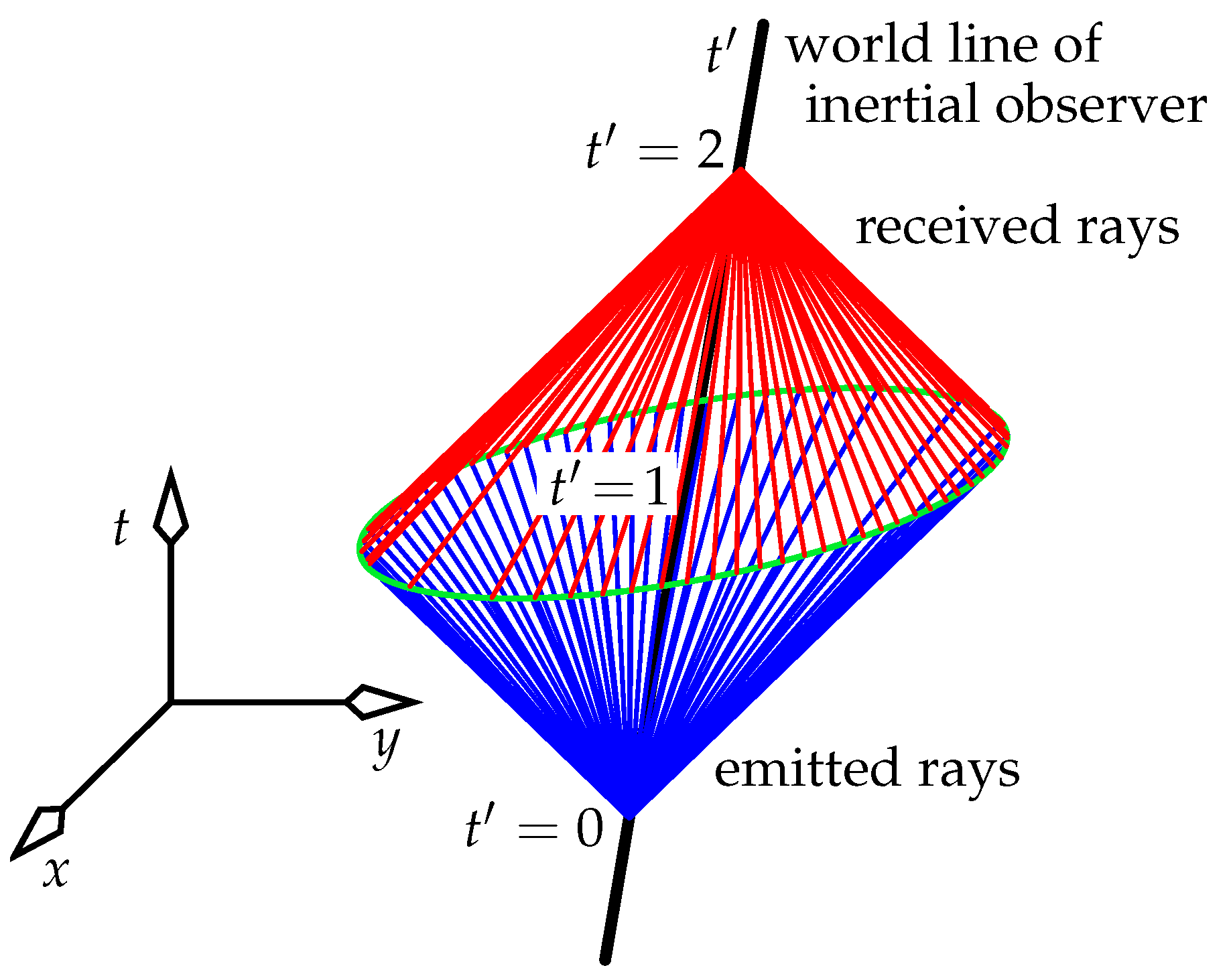
We can also construct this plane of simultaneity without appealing to the Lorentz transform, by extending the one-space-dimensional light-ray construction of Figure 1 to two space dimensions, shown in Figure 6. The primed observer (black world line) emits beams in all directions at , and records all events that reflect these beams back to reach him at on his clock. These events are then all labelled “”, and are defined by the primed observer to be simultaneous with his own clock displaying .
By symmetry in time, this set of light-bounce events must lie in a plane in Figure 6. This set must then be the result of slicing a cone with a plane: it is the green ellipse in that figure. We can also draw light cones for rays emitted before (after) and received after (before) , to conclude that the set of all events defined by the primed observer to occur at is the entire plane containing this ellipse. This plane of simultaneity is central to the rest of this paper.
4.1. Observers in Rotational Motion
Consider a set of observers fixed to a ring that rotates at a fixed angular velocity in its own plane in the inertial lab. Traditionally, analyses of simultaneity on the rotating ring treat a set of -D MCIFs of its observers. They chain together a set of one-space-dimensional Lorentz transforms from each one of these frames to the next, to construct a “helix of simultaneity” in the lab. But simultaneity is not transitive across frames: if you and I inhabit different frames, then if I say events A and B are simultaneous, and you say events B and C are simultaneous, I cannot maintain a priori that A and C are simultaneous. And yet this is precisely what conventional analyses do when they create a “helix of simultaneity”. They draw a cylindrical piece of spacetime and “unwrap” it to make a flat sheet—a nonsensical procedure that is supposed magically to turn two spatial dimensions into one. They then draw a straight line of simultaneity on this sheet, and wrap it back up into a cylinder. They follow this helix most of the way around this “world sheet” of the ring and note that it connects timelike events on any world line: clearly a contradiction [19]. The conclusion is that rotation does not produce a valid frame. I maintain that although rotating frames do not exist, it is not for the above reason. First, constructing the above helix simply makes no sense: a -dimensional analysis simply doesn’t apply to a -dimensional scenario. The inertial frames of special relativity have global extent, and the MCIFs that are chained together are of global extent. Hence each includes the entire ring; their spatial extent is not restricted to a small piece of the ring. It is simply not valid to chain together a series of “tiny” -dimensional frames and wrap them around a cylinder in spacetime as a substitute for what should have been done in the first place with global -dimensional inertial frames. When we do apply a -dimensional analysis in this section, we find that a common standard of simultaneity does not exist for all ring observers, and this is why a rotating frame does not exist.
In [6], I have argued that to analyse a disk rotating in two dimensions, we must make the standard assumption for any non-inertial frame, that the plane of simultaneity at any event on the world line of an accelerated observer is identical to the plane of simultaneity of the MCIF at that event. (This is consistent with the footnote in [20].) Light’s speed is isotropic in any MCIF, and so an emitter’s plane of simultaneity in -D becomes the true measure of simultaneity for that emitter, as opposed to a one-dimensional helix.
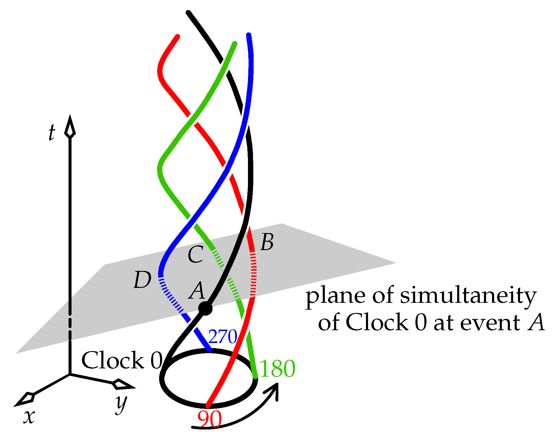
Figure 7.
Reproduced from [6]. A set of helical world lines of four clocks on a rotating ring. Clock 0’s grey plane of simultaneity at the black-dot event A is shown, constructed by the procedure of Figure 6. It intersects the three world lines of Clocks 90, 180, and 270 at events respectively.

A typical plane of simultaneity for a clock on a rotating ring is shown in Figure 7. We see the helical world lines of four clocks fixed to the ring at 90 intervals. The ring rotates in the inertial laboratory of the figure. Suppose these four clocks have been synchronised in the lab: this frame says that at all lab times, the four clocks all display the same value. But the clocks themselves give different meanings to “now”. Clock 0’s world line is black in Figure 7; similarly, Clock 90 has a red world line, and so on. We construct Clock 0’s plane of simultaneity at event A where it displays time zero, and find the intersection events of this plane with the world lines of Clocks 90, 180, and 270 respectively. Event B occurs in the laboratory future of A, event C occurs at the same lab moment as A, and D occurs in the lab past of A:
For example, suppose the ring is Earth’s equator, “spinning east” in the ECI, but with no gravity present (as we are doing a special-relativity analysis here). The above four clocks are always synchronised in the ECI, which is the inertial frame of Figure 7. Now recall the case in one space dimension, where a line of simultaneity for an observer of velocity v has a slope on a -versus-x spacetime diagram of . In two space dimensions, the plane of simultaneity has the analogous tilt in spacetime; thus, as it extends on Earth approximately a distance R (Earth’s radius) to Clock 90’s world line, it rises along the time axis by . The helical world lines of the comparatively slowly rotating clocks on Earth’s Equator (speed 465 m/s in the ECI) are almost parallel to the t axis of Figure 7 [proof: see the analysis around (6)]. This rise is then
Hence, when Clock 0 displays (event A),
- –
- Clock 90 displays approximately 33 nanoseconds (event B),
- –
- Clock 180 displays 0 (event C), and
- –
- Clock 270 displays ns (event D).
(Note this is not the Sagnac effect, since the Sagnac effect involves time differences that increase linearly with longitude, and incorporates no relativity.) If the four clocks have identical ages in the inertial frame, Clock 0 says “Clock 90 is the oldest, Clock 180 has the same age as me, and Clock 270 is the youngest”. This is all very well, but clock 180 constructs a different plane of simultaneity, and concludes “Clock 90 is the youngest, Clock 0 has the same age as me, and Clock 270 is the oldest”. The clocks cannot agree on simultaneity, and this is the reason that they cannot form a frame.
In the inertial frame (in which these clocks are moving with “gamma factor” ), the clocks’ proper times increase at a rate equal to the inertial frame’s clock rate reduced by a factor of . As time passes, each of the clocks says that the other clocks maintain the above time differences relative to itself. In particular, Clock 0 can do a one-off recalibration of them all to display the same time as Clock 0: subtract 33 ns from Clock 90 and add 33 ns to clock 270. This yields a set of clocks whose readings always agree for Clock 0 only. The other clocks on the ring will measure the set to be unsynchronised. But in this highly restricted sense, we now have a kind of rotating frame.
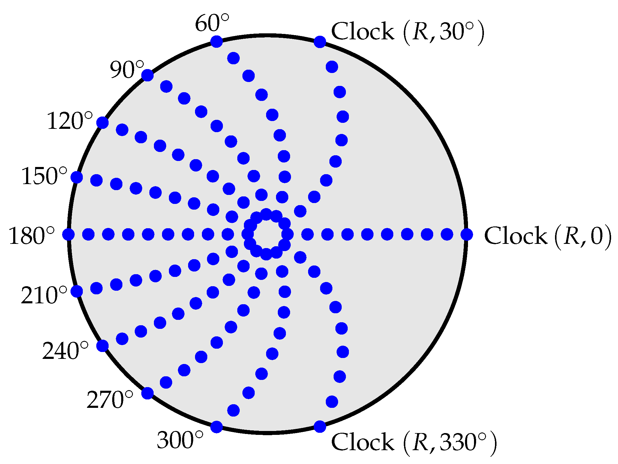
Clock 0’s plane of simultaneity cuts Clock 90’s world line 33 ns into Clock 0’s future. At this moment, Clock 90 is slightly east of exactly 90 from Clock 0, using the degree unit of the inertial lab. Hence Clock 0 measures Clock 90’s angular distance (using the degree unit of the inertial lab) to be slightly greater than 90; the true value for Earth’s size and spin rate is about . Similarly, Clock 0’s plane of simultaneity cuts the world line of Clock 180 such that Clock 0 says that its own time equals that shown on Clock 180 at this moment. Clock 0 then measures Clock 180’s angular distance to be exactly 180. Lastly, Clock 0 measures Clock 270’s angular distance as . Extending this argument to a continuum of clocks fixed to the perimeter, Clock 0 measures these clocks to crowd toward Clock 180. This is depicted later in Figure 14.
Now introduce a set of rulers, each of which links two neighbouring clocks. Clock 0 notes that nearby distances (rulers) on the ring are stretched, and remote distances are contracted. But ultimately all distances are determined by rulers linking clocks; and so we conclude that Clock 0 must measure a circumference of exactly . This simple result hides a complicated spatial metric—Equation (20) in [6]—because for any clock on the ring, a ruler’s length now depends on its position relative to that clock.
From the earliest days of special relativity, researchers have approached rotation by making a rotational Galilei transform from an inertial frame. When treated as a possible change of frame, this transform runs contrary to relativity: after all, central to special relativity is the replacement of the Galilei transform with the Lorentz transform, because the Lorentz transform produces coordinates obeying the relativistic notion of simultaneity. The Galilei transform is a valid change of coordinates, but that does not make it a valid change of frame. Instead, the transform produces a set of what might be called “rotating coordinates” for the inertial frame. These coordinates need have no physical relevance to the rotating system—and they also are not necessarily useful for the inertial frame. In the context of Earth, they are a way of placing ECI coordinates on observers who are fixed in the ECEF, and this is certainly what is done to create our modern world’s “UTC time”. But they are not true coordinates of a rotating frame. My sentiments here echo those of Corum in [21]. Corum decries the use of the Galilei transform—but perhaps doesn’t make the point that this transform is, at best, an attempt to create a set of rotating coordinates for the inertial frame in lieu of the fact that rotating frames don’t exist.
The distinction that I am making here, of rotating coordinates for an inertial frame versus coordinates for a “rotating frame”, is probably completely unknown in the field of precise timing. The oblate Earth with its gravity is a much more complicated example of rotational motion than the above ring. But because analyses of the ring—or rather, rotating disk—have never produced a consensus, we should not expect the subject of precise timing on a rotating Earth to be in any advanced state. This is belied by the analyses found in many precise-timing papers, which simply assume that any arbitrary change of coordinates produces a new frame. See my further comments on this at the start of Section 7.
4.2. Train on Circular Track, the Rotating Ring, and the Pole and Barn Again
Recall the meaning of Born rigidity: a body is accelerated in a Born-rigid way if it is continuously Lorentz contracted while always constituting a frame within which it retains its rest length. Born rigidity is tied to a frame being able to remain a frame once it has been accelerated. If we are willing to drop the requirement for an accelerated vehicle to qualify as a frame, then we can analyse a wider range of motions without demanding any behaviour such as a Lorentz contraction.
Consider accelerating a train in a straight line from rest by firing a set of minuscule rockets, each one attached to one of the train’s atoms, as described in Section 2 and Section 3.3, and shown for two atoms in Figure 3. These rockets are all fired at equal times and by equal amounts in the inertial platform frame. This ensures that the train’s length in this frame remains at its rest length for the duration of the burn, and the burn programme overrides the electromagnetic interaction between the atoms. The passengers say that the rockets fired non-simultaneously in their frame and stretched the train for them by a factor of , producing a new rest length of . In the platform frame, this new rest length becomes Lorentz contracted by to be . So a “rest-to-moving” length contraction by the Lorentz factor of certainly occurs, even though we arranged for the train’s length not to change in the platform frame.
This same idea applies to a train moving at constant speed on the circular track, where the train’s rear carriage is joined to its engine (i.e., this is a model of a rotating ring). The old questions are “Is each carriage Lorentz contracted, or are the links between the carriages Lorentz contracted? What happens to the train’s length?” In the same way that we were free to accelerate the straight train however we chose, and then ask what its passengers observed in the process, we are free to accelerate the train on the circular track however we choose, and then ask what its passengers observe. If we give all of the train’s atoms congruent helical world lines—the most democratic plan—then by construction, it retains its shape and rest length in the platform frame. But the passengers of the train say that the rockets are firing out of order, which stretches some parts of the train and compresses other parts according to the local standard of simultaneity of each passenger. Now they will generally disagree with each other about simultaneity, and hence will not qualify as a frame. So there will be no such thing as a “train frame”.
This, then is the rotating ring of Figure 7. By rotating the ring in the inertial laboratory such that all of its particles follow congruent helical world lines, it is not deformed in the lab, but neither can its observers say that they occupy a well-defined frame. We are at liberty to arrange the world lines of all points in the ring to have any generally timelike shape, and so we might as well treat them all equally, and arrange all to be congruent helices. In that case nothing contracts in the lab frame. This is perhaps the closest that we can get to a “rotating frame” in relativity.
Return to our variant of the pole and barn paradox in Section 2. The pole can certainly be guided into the barn using minuscule rockets and moved in circles indefinitely. But doing so means it will no longer constitute a single frame for the tiny bugs that live on its surface (so to speak). The planes of simultaneity of each of those bugs will be changing wildly, and we cannot treat the entire pole as a single frame in any analysis. (It is certainly not inertial, nor even uniformly accelerated). Any selected bug will observe most of the other bugs on the pole to be older or younger than itself, and will observe the pole to be compressed and coiled up inside the barn; and the barn has not been Lorentz contracted smaller than the pole’s extent. The pole was not accelerated in a Born-rigid way, and although its motion is completely valid, no part of it forms a frame. When the barn door opens, the tiny rockets guide the pole out and can even eventually move it parallel to its length at constant velocity. In that case, from that moment on, it will display the usual Lorentz contraction, and the bugs on it will say that they constitute a single frame.
4.3. The Extent of Disagreement on Simultaneity in the ECEF
In this section we examine the details of simultaneity on a rotating ring by using the example of a set of clocks on our rotating Earth, and satellites orbiting Earth. We focus on their ability to synchronise, given that they disagree on the meaning of “now”. By how much do their versions of “now” differ?
Equation (4) and the discussion around it showed that if clocks fixed at longitudes 0, 90, 180, and 270 all have the same age in the ECI, then in the ECEF Clock 0 will say that in comparison to itself:
- –
- Clock 90 is 33 ns older,
- –
- Clock 180 is the same age, and
- –
- Clock 270 is 33 ns younger.
This relative ageing holds true for all the clocks. In particular, Clock 180 will maintain that the ages of clocks 90 and 270 are the reverse of what Clock 0 says they are. Hence clocks 0 and 180 have a 66 ns disagreement about the ages of clocks 90 and 270. (And similarly, of course, these statements hold true if we swap the roles of the 0/180 pair with the 90/270 pair.) Now replace these clocks by four satellites at the distance of GPS satellites, but all orbiting in one plane and spaced 90 apart. We require the analogous calculation to (4). The satellites are each at a distance of km from Earth’s centre. A satellite’s speed in the ECI is , where G is the gravitational constant and M is Earth’s mass ( SI units). Then, analogous to (4), we write
From the viewpoint of one such satellite, the other satellites’ clocks are mismatched by up to . This has no effect on the operation of satellites that use precise timing, because such satellites are synchronised in the ECI. For example, the calculations that a GPS receiver runs to establish its position are ECI calculations. That is, GPS is based on the ECI time of emission of each satellite signal; it does not use (or even know) the time at each satellite that the receiver says is simultaneous with it receiving a signal.
The above values of 33 nanoseconds and 1.1 microseconds refer to the time that one clocks says is displayed “now” on a distant clock. A different question—but one that is more pertinent to two clocks attempting to synchronise—is the extent to which these clocks agree on the meaning of “now”, since this affects their ability to even define the meaning of the data hand-shake that normally forms part of a synchronisation procedure. To examine how closely two clocks on Earth’s Equator might be able to synchronise in the absence of gravity, we introduce an extra space dimension into the comparison of “nows” in Figure 3. So we calculate the analogous quantity to what might be called Figure 3’s “synchronisation disagreement” of 7 p.m. − 5 p.m. = 2 hours. Note that this is a different task than calculating the one-hour time difference between events A and B in Figure 3, or the three-hour difference between events B and C. A time difference between two observers has no importance if it’s agreed upon by all (such as in an inertial frame), because they can adjust their clocks to correct for it. It only becomes important when observers have different standards of simultaneity: in that figure, Blue says B is simultaneous with A, whereas Red says B is simultaneous with C. No amount of clock adjustment can fix things when observers disagree on simultaneity, since then they simply don’t form a frame.
The two clocks on Earth’s Equator—but without gravity in our analysis—can be envisaged as fixed to a planar ring that rotates in an inertial frame: the ECI in this case. The lines of simultaneity in Figure 3 become planes of simultaneity, such as the one drawn in Figure 7.
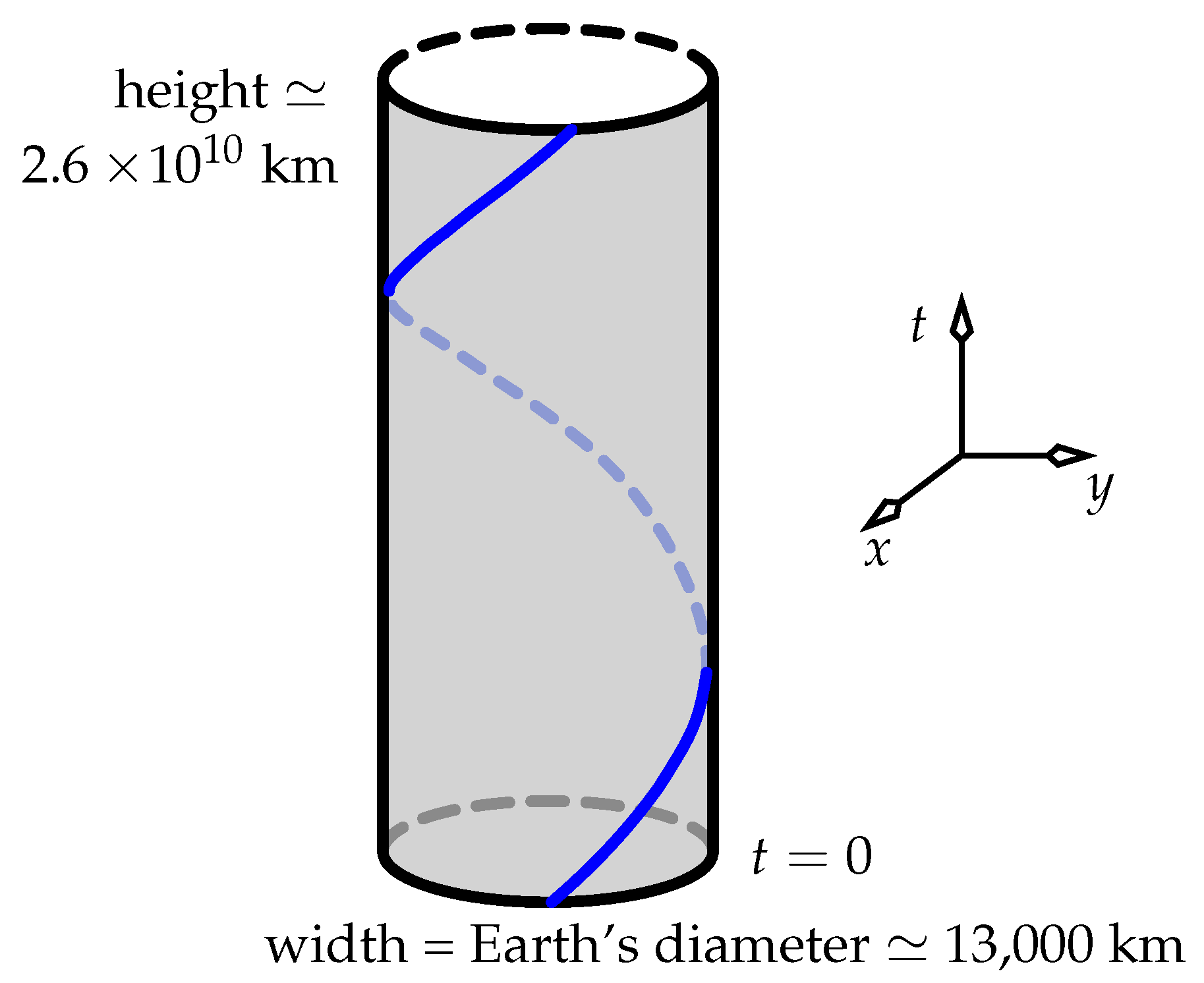
To begin to compare the relative orientations of two such planes, a big simplification can be made. Figure 8 shows the helical world line of a single clock, drawn in the frame of the distant stars over the course of one sidereal day: the time (23 hours 56 minutes) taken by Earth to complete one rotation. The height of the cylinder on which this world line is drawn is
The width of the cylinder is
The cylinder thus has a height-to-diameter ratio of about 2 million. This enables us to approximate the helix as a straight line when analysing sloping planes of simultaneity that encompass a range of ECI times of much less than one day—which is valid here, because (4) gives typical time increments of tens of nanoseconds at most. (A related analysis that uses the exactly helical world lines that are appropriate for any angular speed appears in [6]; but it is far more complicated than the discussion here because it relies on the equations of Section 5, which cannot be solved in terms of standard functions.)
In Figure 9 consider two clocks, Blue and Red, fixed to the Equator. Blue is at longitude 0, and Red is at longitude . (We can ignore the tiny change to their perceived angular separation mentioned in Section 4.1.) Parts of their world lines spanning a small time interval are drawn in Figure 9 around the time in the inertial frame of the distant stars. At this time, Blue is on the inertial frame’s x axis, and its position together with this time define an event A (analogous to event A in Figure 3). At event A we will do the following (depicted in Figure 10):
- Construct the blue plane of simultaneity of Blue (analogous to the blue dashed line in Figure 3).
- Find the event B where this blue plane intersects the red world line of Red (analogous to event B in Figure 3).
- Construct the red plane of simultaneity of Red at event B (analogous to the red dashed line in Figure 3).
- Find the event C where this red plane intersects the blue world line of Blue (analogous to event C in Figure 3).
The difference between the times of events A and C in the ECI quantifies the extent to which Blue and Red don’t share a common “now”. We will calculate this difference.
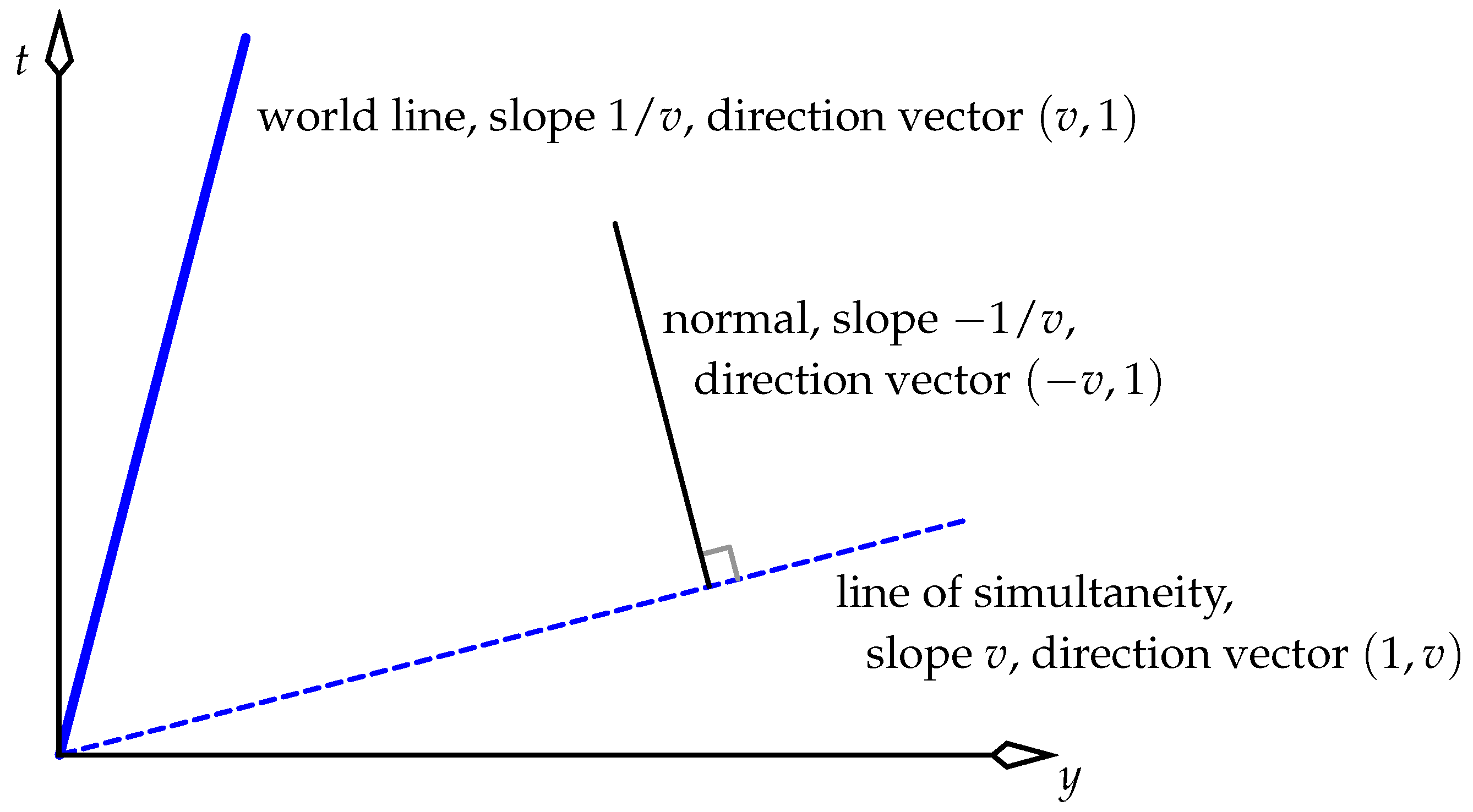
In the equations that follow, we analyse the various planes and gradients using the standard 3-component cartesian formalism of vectors that is ubiquitous in three spatial dimensions. That is, we order the components of coordinate vectors as , because the t axis here takes the place of the z axis in standard geometric analyses of 3-space. The basic tool that we build on is the one-space-dimension picture in Figure 11. The dashed line of simultaneity in that figure is where the plane of simultaneity in two spatial dimensions (x and y) cuts the plane at , at which moment the world line is in the plane, as too is the normal to the plane of simultaneity. Using that idea, start with event A in Figure 10, which has coordinates (for a ring or Equator of radius R)
Analogous to the dashed line of simultaneity with slope v in Figure 11, the blue plane of simultaneity is the set of the following events:
We must find B, where this blue plane intersects the red world line. The red world line—approximated by a straight line—is the set of events
where the parameter takes on all real values, and is a direction vector of the red world line. This vector is found by rotating any direction vector of the blue world line () through angle right-handed around the t axis. Start with
Using the shorthand
we have
Hence, from (10), the red world line has equation
What are the coordinates of event B where this red world line is cut by the blue plane (9)? Substituting the expressions for t and y from (14) into “” gives
Event B’s coordinates now result from placing this value of into (14):
Next, we require the red plane of simultaneity at B. Because we have approximated the blue and red world lines as straight, the red plane’s normal vector is a rotation by of the normal to the blue plane of simultaneity. Referring to Figure 11, start with
Rotate it by to yield
This red plane thus has equation
The constant is found by noting that event B lies on this red plane. Specifically, place from (16) into (19) to yield
Combining (19) and (20), the red plane of simultaneity through B has equation
Last, we find event C by intersecting this red plane with the blue world line. Referring to (11), the blue world line has equation
for a parameter that takes on all real values. Place the coordinates of this into (21) to give an expression for at C:
It follows that
Hence, (22) and (24) give C’s coordinates as
In particular, the third element of (25) is the time of event C in the inertial frame:
Clearly, for (which corresponds to Earth’s natural spin) and , . Recall from (8) that . The difference between the times of events A and C for is called in Figure 10. From now, drop the use of the “” shorthand of (12).
quantifies the fundamental disagreement in simultaneity or synchronisation for clocks that are a longitude apart, fixed to a rotating ring of radius R, and whose speed (in the inertial frame in which the ring’s centre is at rest) is much less than the speed of light, because we approximated the blue and red world lines as straight.
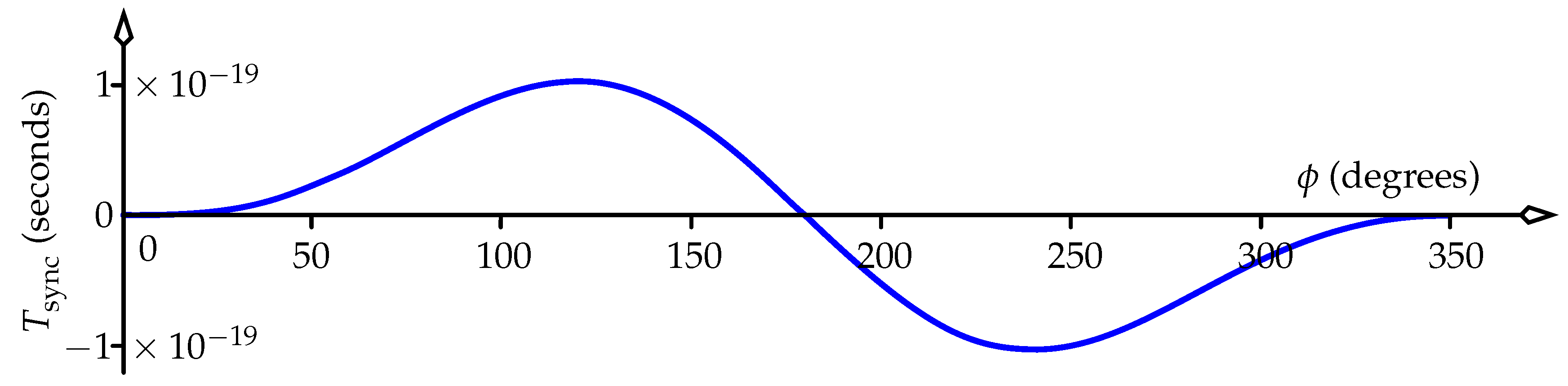
Clocks fixed to Earth’s Equator move at 465 m/s in the ECI. For these, . Hence . Equation (27) becomes
This equation converts to conventional distance–time dimensions by dividing by , where c once again denotes the inertial-frame speed of light:
A plot of versus longitude is shown in Figure 12, using a value of km (Earth’s radius). The maximum value of around seconds occurs at , and it drops to zero very quickly as tends to zero. Indeed, using the small- approximations
it’s clear that for small . Such small values of lie far beyond the accuracy of current communications technology, and so we conclude that a mismatch in the meaning of “now” will have no effect on any synchronisation handshakes currently being made between clocks on Earth.
The above calculation also applies to two satellites in circular orbits in Earth’s equatorial plane, each at a distance R from Earth’s centre. What is the value of for these? Circular motion is sufficient to analyse here, in which case a satellite’s speed in the ECI is . [Note that the satellites’ world lines can be approximated as straight, as the above calculation demands. Also, their speed is far less than the speed of light, and so (28) remains a valid approximation to (27).] Substitute that value of v into (29) to yield
GPS satellites lie at a distance of km from Earth’s centre. Use SI units and choose the worst-case value of . Then
For low Earth-orbit satellites ( km), a similar calculation gives a maximum s.
The above values of say that clocks fixed to Earth’s surface or on satellites have only a tiny mismatch in what they say is “happening now”. This presumably sets a limit to the efficacy of a handshake between their clocks to attempt a synchronisation procedure. But this analysis should not be construed as saying that two clocks for which can be synchronised perfectly. For example, for Figure 7’s Clock 0 and Clock 180 that lie on opposite sides of the Equator (), (29) says that . (This value is easily seen without any mathematics, because the plane of simultaneity of Clock 0 at an ECI time of in Figure 7 will intersect the world line of Clock 180 at the same ECI time of , and vice versa.) Thus events A and C in Figure 10 coincide for clocks 0 and 180. Nonetheless, those clocks do not agree on the time displayed on a clock that is fixed at, say, . Indeed, as stated in Section 4.3, clocks 0 and 180 will disagree on the age of Clock 90 by 66 nanoseconds. Nothing can be done to “fix” this: it is inherent in relativity. So even though is exactly zero for clocks 0 and 180, that only means that they agree on the meaning of “now” at each other’s location; but they disagree at the level of tens of nanoseconds on the simultaneity of events on Earth that are some distance from both of them—and even more so for events far from Earth. But as discussed just after (5), this has no effect on the operation of GPS, because GPS uses the notion of simultaneity in the ECI, not simultaneity local to each clock.
5. Spacetime Coordinates on a Rotating Disk
Consider an event E with polar coordinates in the -D inertial laboratory. We wish to create coordinates for it that are anchored to the rotating disk. We are not interested in the relativistically useless expression in (1). Because the disk is not a true frame, our desired primed coordinates can only have a more limited meaning than coordinates for an inertial frame or a uniformly accelerated frame, whose coordinates give simultaneity and distance information for all observers in these frames. Nonetheless, primed spacetime coordinates can be built that incorporate the ever-changing plane of simultaneity of a single observer on the disk, called the “master clock” here.
Figure 13 shows the disk of radius R. It has been made to rotate using the minuscule rockets mentioned previously in this article, at constant angular velocity in the inertial lab such that at all lab times, the lab distance between every pair of points on it is unchanged from what that distance was before the disk was set into motion. Each point on the disk at any given lab distance from the rotation axis follows a helical world line that is congruent to that of every other point at this distance.
As we know, a disk time coordinate that is consistent with the different standards of simultaneity of all disk observers cannot be defined. But we can partly follow the example of the uniformly accelerated frame, in which the tick rates of all clocks are set such that any clock chosen to be the master clock can say “At the moment that I display any given time, my standard of simultaneity says that all other clocks (by construction) display that same time.” Hence we assign a disk time to an event for which the master clock says “For me, the event occurred simultaneous with my displaying ”. The master clock sets the time on all other clocks to agree with its own, and hence an event can be allocated the time that is displayed on the disk clock that is coincident with it. This is precisely what is done in inertial and uniformly accelerated frames, except that because everyone in those frames agrees on simultaneity, they all agree on the synchronisation of their clocks. In contrast, although the disk clocks don’t agree with each other’s displayed time as per the discussion of Section 4.1, at least the master clock can build a coherent picture of events from its own viewpoint.
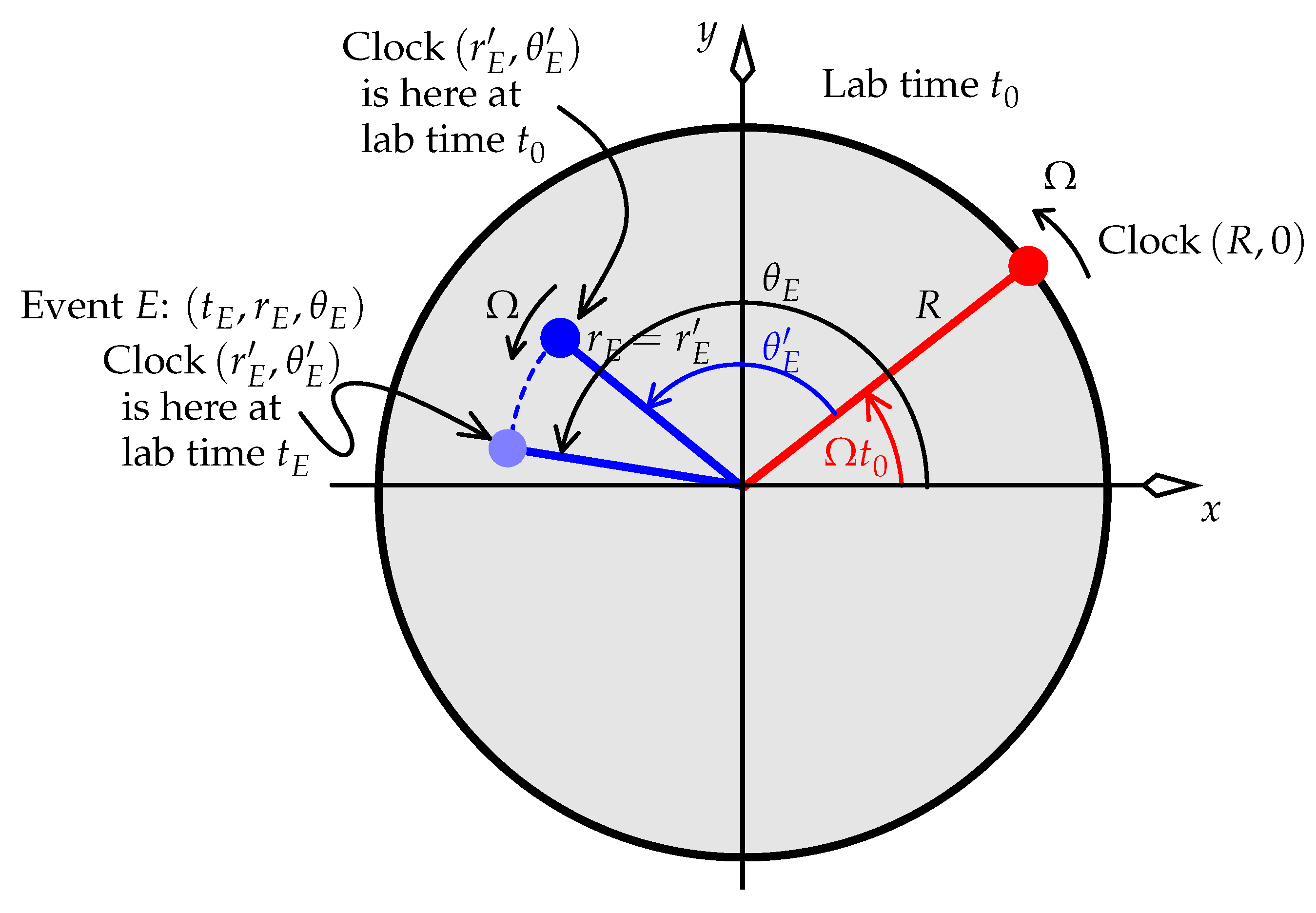
At lab time , the master clock is at lab polar coordinates , and so is labelled “Clock ” for all time. We ask: given R, , and an event E at lab coordinates , what coordinates does the master observer give to E?
At some lab time , the master clock’s plane of simultaneity contains event E. (Refer to Figure 7 to help visualise the situation.) At this moment, Clock has rotated through a lab angle , as shown in Figure 13. Clock ticks slowly in the inertial lab by the usual gamma factor , and so it displays at this lab time . This time is now defined to be the time of event E.
Disk spatial polar coordinates are defined for E using the same procedure employed in basic relativity: when a “primed inertial frame” moves at constant velocity in an unprimed inertial frame, the primed coordinates of an event are the primed coordinates of the primed clock that is present at the event. (The exception to this case here is that we don’t do likewise for the time coordinate, because a global time coordinate cannot be defined; hence we have allocated the master clock’s displayed time to .) Thus, on the disk the polar coordinates of event E are those of the polar-coordinate label of the disk clock that is present at E, which is (by definition) Clock .
It’s clear from the symmetry of the helical world lines that . What about ? Note that
Hence . The sought-after change of coordinates from the inertial lab frame’s for event E to is then
We have yet to determine , the lab time at which Clock says “E is happening now”: E lies on Clock ’s plane of simultaneity at . The following calculation of uses a similar cartesian approach to that of Section 4.3. As in that section, we use here the standard formalism of 3-dimensional spatial geometry: thus, purely for convenience, the time axis is given the role of a third spatial axis in the following 3-vector formalism. In keeping with this, we order the lab coordinates as and not .
Recall that at the plane of simultaneity of Clock contains event E. To find this plane of simultaneity, consider that at , Clock is moving with velocity in the positive y direction. Referring to Figure 11, the plane of simultaneity at has normal vector . At the normal to the plane of simultaneity of Clock is found by rotating that initial normal vector by angle right handed about the t axis:
The right-hand side of (35) is the normal to the plane of simultaneity of Clock at lab time . This plane contains the event describing Clock at lab time . This event has lab coordinates
It follows that the plane of simultaneity of Clock at has equation
because this plane’s normal is [matching the right-hand side of (35)], and the plane contains the event in (36). Now, because we demand that this plane also contain event , (37) becomes at E
This can be re-written as
This supplies the required by (34): recall that was originally specified, not . The complete transform, (34) and (39), resembles Langevin’s Galilei transform in (1), but is fundamentally different because of the presence of .
Equation (39) recalls Kepler’s equation of orbital mechanics, and must be solved numerically for . This need for a numerical solution highlights the difficulties involved with rotating-disk analyses. Although (39) resembles Grøn’s Equation (6) in [22], Grøn’s analysis and conclusions differ from ours. Grøn states that a rotating observer’s standard of simultaneity is identical to that of the lab. In our view, which is built on the rotating observer’s MCIF with its “tilted” planes of simultaneity (Figure 7), that is certainly not the case.
Note that (33) implies
It follows that (39) can be written as
This shows how to calculate the time interval .
The transform (34) with either of (39) and (41) specifies a kind of “pseudo-frame” for the rotating disk. It is studied extensively in [6], and some of the results that follow from it there are outlined in the rest of this section.
5.1. How Clock Observes the Disk
The discussion in Section 4.1 makes it clear that Clock will observe (not “see”) the clocks fixed to the disk to be shifted towards its antipodal point. A precise calculation of the amount of shift is given in [6]. Figure 14, taken from [6], shows a typical result for a disk of radius m spinning at .
Clock observes the disk clocks to crowd toward the opposite side of the disk, so that nearby rulers that connect disk clocks are stretched, and distant rulers are compressed. But each of these rulers defines a unit of length in its neighbourhood. Hence “unit rulers” fit around the periphery, as they do in the lab. So Clock says that the disk’s circumference is .
5.2. Resolution of the Circular Twin Paradox
The above formalism allows an analysis of the “circular twin paradox” [16]. Figure 15 shows twins Alice and Bob, counter-rotating at equal but opposite angular velocities in the lab, at equal lab distances from their common centre of rotation. They always have equal ages in the lab, and so each time they meet they must agree to having equal ages. How does each twin describe the scenario?
This scenario is a -D version of the well-known -D scenario in which Alice and Bob accelerate away from each other in the lab for a fixed lab time, then reverse direction to reunite, such that their lab speeds at each lab moment are identical. This situation is well understood: to draw, say, Alice’s version of events, we simply construct her line of simultaneity at each event on her world line in dimensions. Its intersection with Bob’s world line at any given moment for Alice tells Alice how old Bob is at that moment. The undisputed result is that Alice says Bob is ageing slowly on their departure, quickly when he is far away from her near their “bounce”, and slowly once again at their reunion. The result is that their ages are equal—as expected—at the end. This result makes clear the well-known fact that the tick rate of a clock in an accelerated frame depends on its position in that frame.
A description of this scenario using the primed coordinates in (34) and (39) was given in [6], to which we refer you for details. The scenario can be related to the rotating disk formalism via Figure 15. There we see Alice aged at lab time , and she asks what age Bob has at this moment. The event of Bob’s age being measured occurs at some lab time t, when Bob is aged . Reference [6] gives the necessary calculations. A plot of Bob’s age versus Alice’s appears in Figure 16. Alice observes (not necessarily sees) Bob to age slowly as he recedes from her. She observes him to age quickly around his farthest point from her, and then to age slowly once more on his return. When they meet, they indeed have the same age, as expected.
Whereas the -D scenario deals with well-defined frames (albeit accelerated), the circular scenario does not. Nonetheless, the description of the circular scenario really follows the same idea as the -dimensional case, shown earlier in Figure 4. In contrast, the authors of [16] construct different definitions of synchronisation, and conclude that “The resolution of the paradox [...] depends on the method that is used to synchronize clocks on a ring”. Aside from the fact that there is nothing paradoxical here that needs resolving, the more important point is our statement in Section 3: synchronisation is not an arbitrary procedure that we can redefine to eliminate some perceived difficulty.
5.3. The Speed of Light Around the Disk’s Periphery
The rulers linking adjacent clocks define the spatial metric on the disk. We can envisage a “unit ruler” to be one that connects any two adjacent clocks at the same radial coordinate in Figure 14. (Of course, a proper derivation of the metric uses rulers of infinitesimal length.) Following Figure 14, each observer says that nearby rulers are stretched and distant rulers are compressed. We can use this idea to calculate the coordinate speeds measured by Clock of two light signals sent around the disk. At lab time 0, Clock emits two signals. Signal “E” heads “east” toward clock in Figure 14. Signal “W” heads west toward clock . The coordinate speed of each signal is the number of “unit rulers” it passes in a unit of Clock ’s time , where Clock has lab velocity .
The expressions below are calculated in [6]. A signal (or object) runs along a circle of radius R in the lab, with a constant lab velocity of . Clock measures the signal’s velocity at the moment of emission to be
As a check, consider the case where all speeds are much less than the speed of light: V and are much less than 1. Equation (42) reduces to the expected galileian result:
In particular, light signal E has velocity 1 (i.e., c) in the lab: . Equation (42) then gives its velocity measured by the emitter as . Light signal W has , yielding . The emitter thus measures both signals to have speed (i.e., ) just after they were emitted. If the emitter inhabits a true frame (even non-inertial), it must measure both signals to have speed 1 in its vicinity; but recall that a well-defined “rotating frame” does not exist. Analogously, an inertial platform says that a constant-velocity train’s clocks tick slowly by , and the train’s rulers are contracted by . These two factors end up cancelling in a way that makes the train’s passengers measure light’s speed to be 1 everywhere along it. But in the case of the rotating disk, although the inertial lab says that the disk clocks tick slowly by , it says that the disk rulers are not contracted at all in the lab. There is no ruler-contracting to cancel the disk clocks’ time-slowing . This imbalance of gamma factors leads to the emitter Clock measuring light’s speed locally to be and not 1.
What does the emitter determine the two signals’ velocities to be when they are on the opposite side of the disk to the emitter? Reference [6] gives these velocities as
(Velocities for intermediate positions of the signal are also given in [6].) For low V, both signals start out with speed approximately 1. The eastbound signal slows until it reaches the opposite side of the disk, then speeds up as it returns to the emitter. The westbound signal speeds up considerably until it reaches the opposite side of the disk, then slows on its return.
5.3.1. Comparison of (44)’s Signal Speeds with the Sagnac Effect
For small V, suppose we make the simplifying assumption that the average speed of each signal E and W around the rim according to the master-clock emitter is approximately the mean of two values of : one at the emitter’s location, and the other on the opposite side of the disk from the emitter. For signal E, these speeds were given above in the discussion around (43) and (44) to order V as 1 and respectively; hence its average speed is approximately . Similarly, the emitter says that for small V, signal W has an average speed (not velocity) of .
These low-V average speeds can be derived in a standard way from an inertial-frame analysis of the Sagnac effect. Work to first order in V, hence ignoring factors of here. We emphasise the fact that the Sagnac effect is fully non-relativistic by writing the speed of light as c instead of 1. The emitter knows nothing of the above analysis. It simply says that the round-trip average speed of an eastbound light ray is , where is the ray’s round-trip time measured in the inertial lab. The lab says that at the moment when the eastbound ray “laps” the emitter,
That is, . Hence . The emitter then uses this value of to write (without using any relativistic analysis)
The emitter also sends a signal west, and calculates the ray’s round-trip average speed as , where is the round-trip time in the lab. In the inertial lab the westbound signal only traversed part of the circumference before the emitter had moved some way east and collided with it. The lab then says
Thus . Hence , and so the emitter concludes
The above very-conventional Sagnac calculation essentially mixes inertial and non-inertial frames. It combines the motions of signal and observer in the inertial lab, but the non-inertial observer fixed to the disk states that the total distance travelled by each signal is in the lab time or .
The two Sagnac signal speeds cause some to claim that relativity is “incorrect because these speeds differ from c”. But of course that claim is nonsense, since a speed of c is only necessary in an inertial frame.
The standard Sagnac speeds produced by the above non-relativistic analysis are global averages, because they equal “total distance over total time”; hence they have no dependence on angle traversed (that is, on the location of the signal). They agree with the small-V average values of in Section 5.3’s relativistic analysis. A lab on Earth’s Equator has a velocity m/s in the ECI. Thus, when light signals are sent east and west from a lab on Earth’s Equator, the eastbound (westbound) pulse of light will take 207 ns longer (shorter) to return to the lab than it would if Earth were not spinning. (The Sagnac effect can thus be used to measure an object’s spin rate, making it useful in modern inertial navigation systems.) Because the Sagnac speeds are global average values, the emitter cannot conclude that the eastbound light ray has a constant speed. And indeed, we have seen in Section 5.3 that the relativistic-disk analysis says that the speed actually varies between c and for .
This angular dependence of the signal speeds in the relativistic-disk analysis eliminates “Selleri’s paradox”. In [23,24], Selleri assumed that the Sagnac speeds of are global constants, not global averages. Hence, he reasoned that they must be measured locally by any observer. He then argued that by taking in the Sagnac analysis while keeping V fixed—meaning the disk’s angular velocity would become arbitrarily small—these same two speeds would be observed in a frame that was arbitrarily close to being inertial, moving at speed V in the inertial lab. This produced his paradox, since relativity requires both signals’ inertial-frame speeds to be c rather than . But the rotating-disk analysis around (44) makes it clear that Selleri’s are not global constants: in particular, they do not apply at the emitter. Locally, the emitter measures the value given in (42). As shown just after (43), this equals [or c to order ] at the emitter for both eastbound and westbound rays. The discussion after (43) explains why this value is not exactly equal to c. To recap, the rotating disk in this paper is spun rigidly in the lab using guiding rockets, and hence no length contraction exists on it. This absence of length contraction—which produces the in the speed “ ”—is preserved in the large-R limit described by Selleri.
We see here that the speed of light is predicted to be in a laboratory fixed to Earth’s surface, where is set by Earth’s rotational speed in the ECI, where Earth turns once per sidereal day. The speed of a point fixed to the Equator is 465 m/s in the ECI, and so the maximum value of for all latitudes—which is on the Equator—is approximately . The speed of light measured in the lab is thus predicted to differ by only 1 part in from the value 299,792,458 m/s. Laboratory experiments from the 1950s onwards have measured the speed of light to within tens of metres of the modern value of c, and the 1972 value of Evenson et al. was 299,792,457.4 m/s [25]. These have presumably all been two-way averaged speeds. The literature of one-way measurements is large. Maxwell’s theory predicts that light’s speed in an inertial frame is isotropic: it has a one-way speed, and that equals its two-way speed. So, if we were to believe Selleri’s statement that the Sagnac speeds apply to any location on the spinning disk, we would be forced to claim that light’s one-way speed must be measured in the lab to differ from c by up to some hundreds of metres per second. Experiments contradict that claim.
5.4. Alternative Derivation and Comments on the Sagnac Effect
Here is an alternative derivation of and in Section 5.3.1 that gives insight into a related area of relativity: the question of a bona-fide change of frame versus a trivial change of coordinates. We set for the start of this discussion.
Consider the -dimensional laboratory’s flat-spacetime metric in polar coordinates:
The simplest Sagnac scenario that we are analysing has , the disk radius: we are concerned only with events on the disk rim. Hence the squared proper time between neighbouring events on the rim is
For light running along the rim, , and so lightlike events have
Suppose light traverses a lab angle around the disk. For eastbound travel , and (51) becomes
The lab time taken for its trip ( in Section 5.3.1) is . Consider this travel in a somewhat galileian way: as the light pulse traverses the rim, in a time it gets “carried along” with the disk (which has angular velocity in the lab); plus, it traverses a tiny amount of the total angle . Then its angle traversed in the lab is
We emphasise that this picture is galileian: it assumes the light is carried along with the disk at the speed of the disk, which we know is not really true: after all, a light ray traversing a stream of water is not carried along with the speed of the water.8 Equations (52) and (53) combine to give, with as used throughout this paper,
It follows that
The time for the eastbound light pulse to traverse one circuit on the disk is then
The analogous time for westbound light, , can be calculated from the same procedure by imagining the disk to be spinning the other way. The result of that is the substitution in (57):
These match the values given in Section 5.3.1. The important point here is that despite the use of a metric in (49) and the (Galilei-) transform appearance of (53) (or more specifically, its non-infinitesimal version ), the above procedure was not some kind of “relativistic transform to a rotating frame”. Rather, (53) created the angular coordinate of what we might call a set of “rotating coordinates” in the inertial lab. That is, defining rotating coordinates in an inertial frame is not the same as defining coordinates in a “rotating frame”. The former coordinates were created in the equations of this section; the latter simply don’t exist.
Nonetheless, the above procedure appears in a more convoluted form in Section 6 of [26], where it is applied to the rotating Earth. That reference touts the above procedure as a transform from an inertial frame (the ECI, equivalent to our lab) to a rotating frame (the ECEF), and constructed on the non-infinitesimal version of (53), (written in [26] as with ). That reference also incorrectly assumes that relativity is built in to its analysis, just because a metric appeared. But we see here that the above procedure neither contains relativity nor is a transform to a rotating frame. It is simply a galileian coordinate transform wholly within the ECI. Section 7 discusses this further.
6. Clock Rates on the Real Earth
Up until now, this paper’s analyses have used special relativity only. This section adds a refinement to the prediction of the local speed of light in Section 5.3 on the disk, when gravity is included for a clock fixed to the real Earth.
In Newton’s theory, the gravity field of a sphere whose density is a function only of distance from its centre is unaffected by whether the sphere rotates. Conventionally, this non-relativistic idea is used to model an Earth-fixed clock’s timing as that of a clock moving in the gravity field of a non-rotating Earth. Such a field is described up to standard levels of accuracy equally well by the weak-field and Schwarzschild metrics. These metrics were tested experimentally in the famous Hafele–Keating experiment of the early 1970s, in which the timing of clocks flown around the world for some days was measured and found to agree with this non-rotating-Earth model to the level of about one standard error, around 10–20 ns.
But, strictly speaking, the weak-field and Schwarzschild metrics are not those of a rotating body. So although these metrics are adequate to describe a situation such as that of Hafele–Keating, they are not necessarily good enough to model precise timing, where we require accuracies of 1 ns or better over the course of several days. In fact, no solution to Einstein’s equations of gravity is known that applies with ultra-high accuracy to clocks fixed to the rotating Earth (or even a rotating spheroid). The Kerr metric might be considered: the Kerr and Schwarzschild metrics are both vacuum solutions of Einstein’s equations, describing a universe that contains a point mass but is otherwise empty. Unlike the Schwarzschild metric, the Kerr metric allows the point mass to have angular momentum. But whereas Birkhoff’s theorem says that the Schwarzschild metric also describes the gravity field external to a non-rotating spherical mass of non-zero radius, no analogous result is known that relates the Kerr metric to the gravity field external to a rotating mass of non-zero radius. The bottom line is that no solution to Einstein’s equations is known that describes the details of ultra-high-precision timing of clocks fixed even to a rotating sphere or spheroid, let alone to the real rotating Earth.
The simultaneity that was used throughout this paper to discuss precise timing is built on what we can infer from signals of constant speed being exchanged between two clocks. In non-inertial systems, light’s speed is a function of its position. That turns out not to impede simultaneity being defined in the uniformly accelerated frame via MCIFs—albeit with some work required. But when gravity is introduced and spacetime becomes curved, the concept of simultaneity becomes problematic. General relativity does not give any prescription for what simultaneity means; it’s only in the absence of gravity that we can use the constancy of the speed of light to form a natural idea of what it means to say that some event is happening “now” somewhere else. Hence general relativity currently gives no prescription for how two clocks might be synchronised. (It is often said that the GR allows arbitrary foliations of spacetime into surfaces that can define simultaneity. I suggest that with such arbitrariness, simultaneity loses all meaning, and so the surfaces do not define simultaneity.)
These problems aside, in this section we will attempt to combine a weak-field calculation of the speed of light near Earth’s geoid with the fact that Earth rotates. The geoid is a mean sea level over the planet: it is an equipotential surface, where the equipotential combines gravity with a centrifugal term for observers at rest on the geoid, who thus rotate with Earth in the ECI.
Envisage clocks A and B, both fixed to the geoid, meaning rotating with Earth but otherwise at rest on Earth’s surface. Clock A sends a light signal to clock B. Because A and B are relatively at rest, when B “looks” at A (that is, records and analyses the light signal from A), no Doppler shift is present to complicate what is seen. Thus, A’s tick rate as seen by B is no optical illusion. Rather, it is “really happening”: it is the tick rate that B measures A to have. Additionally, because Earth’s geoid is an equipotential surface, no work is done on or by a photon travelling from A to B, and hence the photon’s frequency is unchanged from emission to reception. It follows that B measures A to be ticking at the same rate as B. We conclude that all clocks fixed to the geoid tick at the same rate.9 This common tick rate of clocks at rest on the geoid is called International Atomic Time (TAI), denoted T here. It is what accurate clocks on Earth measure. Its base unit is the SI second.
We wish to calculate , the speed of light “near” the geoid with reference to TAI, where by “near” we mean that the light moves as close as possible to the geoid, but at a fixed radial distance from Earth’s centre and along a fixed latitude. Begin by modelling spacetime in Earth’s vicinity by the weak-field metric in Schwarzschild spherical polar coordinates :
Here is the proper time between any two infinitesimally separated events at , and is the dimensionless gravitational potential at the point with no centrifugal contribution (that is, is the usual potential divided by ). In these coordinates, a circle of radius r has circumference —which is desirable for discussing our oblate spheroidal Earth. What is the meaning of the coordinate t? At a stationary clock at spatial infinity () the potential tends toward zero, and (59) becomes . The coordinate t thus measures the proper time elapsing on that motionless clock at spatial infinity.
To define , we follow a photon that moves at constant and that are as close as possible to the geoid. The photon traverses an angle in a time . Hence
We will evaluate this by setting in the metric (59), but will first eliminate the metric’s in favour of , since is referenced to TAI time T. TAI time is that of a clock fixed to the geoid and rotating with Earth. So, suppose this clock moves at and , and traverses an angle in a time . With the potential on the geoid, we have
The velocity of this clock fixed to the geoid is, in the ECI (that is, referenced to t)
Note that on Earth’s Equator, the dimensionless and are and respectively. This knowledge allows us to invert (62) to first order in and , yielding
This expression for inserts into the metric (59) to replace with :
For light on the geoid, setting in (64) gives
Rearrange this to yield
Referring to (60), we infer that to first order in and . We might approximate this result (which assumes small V) by , the gamma factor for the speed V. That is, at a low angular rotation rate, gravity increases light’s speed by a factor of on the geoid. In Section 5.3 we showed that in the absence of gravity, an observer on the rotating Earth measures light to have speed locally. We now see that in the presence of gravity, this observer will write
This is an intriguing result: it says that if we introduce the weak-field metric into this paper’s discussion of simultaneity in rotation, gravity exactly annuls the effect of rotation on light’s speed, at least for an Earth that rotates slowly in the ECI.
7. A Critique of Precise-Timing Literature
I close this paper with some comments on what I see as a status quo in the precise-timing community that will struggle to meet the demands of increasingly accurate synchronisation. Journal papers in precise timing are not always written by relativity specialists, since those papers can treat their relativity naively or even incorrectly. My criticism is not new; see Corum’s critique [21] of a paper on simultaneity and precise timing by Winkler [28]. Corum points out the common misperceptions of relativity found in Winkler’s paper. Besides such for simultaneity, he notes the frequent use of tensor notation masquerading as general relativity more generally in timing papers. Unfortunately, too few academic relativists appear to have enough interest in precise timing to fix such problems before they are published.10
7.1. TAI and the Date Line
Reference [27] states, without giving details, that a suggestion has been made that a need exists for a discontinuity in TAI to be placed at the International Date Line. I argue here that any such suggestion is based on a faulty application of relativity to precise timing. (The fact that TAI incorporates gravity is irrelevant to the current discussion, since the same ideas apply to clocks fixed to the edge of a massless disk rotating in an inertial frame far from any gravity.)
First, return to the clocks shown in Figure 7. These are fixed to the edge of a disk that rotates in an inertial frame, and can be treated as fixed to Earth’s Equator, which rotates in the ECI. If the clocks are all synchronised in the ECI, then individually they will disagree on simultaneity. The Lorentz transform describing the MCIF at each event on the Equator produces a set of planes of simultaneity, one of which is shown in Figure 7. This plane results from applying the -D Lorentz transform to the MCIF of Clock 0 at event A; it is the approach used in [6] and is the bread and butter of special relativity: constructing MCIFs and Lorentz transforms. In Figure 7, with all clocks synchronised in the ECI, when Clock 0 displays time 0, Clock 0 says that Clock 90 displays 33 nanoseconds, Clock 180 displays 0, and Clock 270 displays nanoseconds.
What if we use more clocks? Place 360 of them 1 apart around the disk’s edge, labelled “Clock 0” to “Clock 359”. The approach of using planes of simultaneity subsumes the idea of lines of simultaneity, and so the standard arguments of constant-velocity motion say that clock n maintains that the nearest clock to the east, clock , displays ahead of clock n by approximately , where m/s is the clocks’ speed in the ECI and L is their separation. Hence, Clock 0 says that clock 1 displays ahead of Clock 0 by ns. Similarly, clock 1 says that clock 2 displays ahead of clock 1 by 0.576 ns. This is well and good, but simultaneity isn’t transitive: we cannot conclude here that Clock 0 says that clock 2 displays ahead of Clock 0 by ns. The reason is that when the clocks no longer share a common (or approximately common) velocity, we require a two-space-dimensional analysis, and that involves planes of simultaneity that allow Clock 0 to make a statement about clock 2 that is not simply related to clock 1. Hence, for example, Clock 0 says that Clock 180 displays the same time as Clock 0, and certainly not ns into the future.
In contrast, the standard approach in rotating-disk literature to this set of clocks has been to chain together the above 0.576 ns differences, and so conclude that every clock is, in a sense, under duress to display ahead of itself.11 (See my comments on global versus local simultaneity near the start of Section 3.) That this conclusion is obviously contradictory is supposed to show that clocks on a disk cannot be synchronised. One of the aims of this paper has been to show that although the above chaining argument is faulty, its conclusion is correct. The argument I have proposed is not more difficult, but requires the proper -D analysis of Section 4.1, that uses global planes of simultaneity of MCIFs.
It’s clear that the above-mentioned discontinuity in TAI at the Date Line would be a disaster, because the very existence of the above 207 ns discontinuity is based on a wrong application of relativity: namely, applying transitivity to a chain of -D Lorentz transforms, when instead relativity calls for a single -D Lorentz transform for each observer, which produces no build-up of time going around the Equator. Certainly clocks cannot be synchronised in any sort of “ECEF frame”, and yet for every observer in Figure 7, no discontinuity exists; the problem is only that different observers have different standards of simultaneity. Relativity makes no excuses for this disagreement in simultaneity, and making TAI discontinuous along some chosen meridian will not “fix” that. Nothing here needs fixing.
7.2. Coordinates versus Frames, and Misguided Metrics
An important question asked in this report (see, for example, the discussion near the end of Section 5.4) is: “When does a coordinate transform equate to a bona-fide frame in relativity?” Suppose we take the metric for flat spacetime in one space dimension, , and make a Galilei transform
The metric that results,
clearly does not describe a true relativistic frame; it’s simply an exercise in changing coordinates. In contrast, if we make the usual Lorentz transform, the resulting metric does describe a true relativistic frame. Unlike the Galilei transform, the Lorentz transform produces a time coordinate with the property that events with the same value of that time coordinate are simultaneous in the relevant frame—which is precisely what a good time coordinate should do. But how are we to know which metric describes a bona-fide frame, based purely on inspecting the metric? I believe this is a key question in relativity, but I am not aware of it being addressed anywhere. It cannot be waved away simply by redefining simultaneity as describing two events that have the same time coordinate, when this time coordinate has merely been constructed in some arbitrary way to suit the task at hand. Such a redefinition carries no real physical meaning, because in applying it, any two spacelike events could be arranged to be called simultaneous, and the concept of simultaneity would become empty. Indeed, placing the Galilei transform on a par with the Lorentz transform runs counter to the very existence of the field of relativity. Simultaneity runs far deeper than merely defining coordinates. It is defined by the behaviour of light in a well-known way, and is extended as best as possible to non-inertial frames by the use of MCIFs.
This distinction between a coordinate change and a frame change seems currently to be absent from the field of relativistic precise timing. Our world’s global UTC time is TAI time with leap seconds included: these are an occasional correction for the fact that a whole number of TAI’s seconds don’t quite match Earth’s day/night cycle. TAI is the time coordinate of what might be called a “rotating set of ECI coordinates” that are currently used in the ECEF to define TAI/UTC (with general-relativistic modifications included—but these are secondary to the problem of rotation). But these rotating ECI coordinates are not a fully relativistically meaningful set of ECEF coordinates; they are just the best that we currently can do, since a true ECEF does not in exist in relativity. In years to come, as clocks become ever more precise and networks connecting them expand, I think that this lack of understanding of the distinction between a global time and the simultaneity standard of any given Earth-fixed clock is set to create contradiction and confusion in the relativistic precise-timing community. The discussion of TAI and the Date Line in Section 7.1 suggests that this confusion already exists.
A good understanding of special relativity is necessary to analyse simultaneity. But special relativity currently lacks a profile in most universities, where academic relativists are expected to devote their time to the more bankable subject of general relativity. General relativity is usually said to incorporate special relativity, but it must be said that GR is of no help when we analyse any of SR’s standard textbook paradoxes; nor does GR help us create coordinates for the rotating disk in flat spacetime. The languages of GR and SR are very different, and familiarity with one of these fields does not imply or impart familiarity with the other. Writing a metric down does not imply that some deep GR analysis is being made.
It is worth highlighting here the result of a recent survey [29] that demonstrated a poor understanding of basic special relativity even among academic physicists—despite those physicists rating themselves as highly confident of the correctness of their wrong answers to the survey questions. For example, any number of physicists in academia (and many hobbyist web sites) still make the most basic of mistakes by confusing relativity with the Doppler effect.12 Such misunderstandings of the basics can be worsened by pseudo-analyses that sometimes appear. Witness [30], which presents a series of illogical and vacuous steps to conclude that one of special relativity’s core physical concepts—the equivalence of mass and energy—is trivial, empty algebra devoid of any physical content. It is disconcerting that a century after the birth of relativity, reputable journals still publish such arguments.
The lack of a strong connection of universities to special relativity means that academic relativists generally have little interest in SR, have no time to devote to it, and no appreciation of its difficulties and subtleties. (Indeed, a common response of academic general relativists to questions of precise timing seems to be “I’ve no idea, but I’m sure that if you do it properly using GR language, it will all work out.”) Of the academics who work on SR or GR, only a small fraction have an interest in precise timing. That subject then becomes dominated by non-relativists, and suffers.
The errors in understanding that appear in precise-timing papers cover the full gamut of special and general relativity. A case of incorrect special relativity appears in [26]’s discussion of the speed of a signal in an inertial frame. In a straightforward scenario whose infinitesimals (predictably) obey the Lorentz transform (although that expression does not appear), that reference sets equal to (to order v). This is clearly incorrect, since the discarded term is central to the discussion. Although the resulting expressions are broken, their accompanying discussion is contrived to arrive at known expressions. Indeed, were the Lorentz transform to be used from the outset, the correct result would emerge in just a few lines of algebra. This is a classic example of a precise-timing analysis that appears on the surface to derive well-known results, and yet makes no sense at all.
Also in the field of special relativity, the subtleties of simultaneity in the context of accelerated frames, which are well known in relativistic circles and are central to a proper understanding of special relativity (emphasised, e.g., by analyses of the twin paradox), are simply rejected by fiat in [10]. That reference uses the valid concept that any coordinates can be used to quantify a scenario, to insist that observer-dependent simultaneity is irrelevant to relativity and timing. This flies in the face of relativity and timing.
For two examples of misunderstandings in general relativity, consider first page 44 of [27], which states that observers at rest on Earth attribute the special-relativistic slowing of time on a clock that moves over Earth’s surface to “the warping of spacetime due to spacetime terms in the general-relativistic metric tensor”. It’s not at all clear what the “spacetime terms” are; but aside from that, those observers would still detect such a slowing of time on the moving clock if Earth were hollow and thus spacetime were flat. Hence curved spacetime plays no role here: if spacetime is curved for some observers, it is curved for all observers, and if it is flat for some observers, it is flat for all observers. The cited statement appears to say, incorrectly, that spacetime curvature is observer dependent.
A second example in GR is what seems to be a widespread misunderstanding of the metric tensor in the precise-timing community, in [31]’s equation (5.49) and similar equations. This writes what it calls “the metric tensor components in the ECEF up to terms of order ” in a notation that is equivalent to the following:
How this metric has been produced is not made clear in [31], although it seems to be a combination of (69) and the weak-field metric (59).13 In particular, the space part of (70) has no gravitational contribution, and yet this contribution is clearly present in the weak-field metric. The point here is that we must know the relative sizes of the time and space infinitesimals in (59) to be able to write a “ approximation” to a metric. A metric concerns all events in spacetime, and we can only omit terms in an integral of the proper time along some world line when we have applied the metric to the events on that world line. A metric such as (70) is, at most, only relevant to a specific set of events—ones that are connected by a slow-moving object—and yet it is incorrectly described in [31] as an approximation to the metric of all spacetime. Indeed, many papers in precise timing roll out spacetime metrics as if the inclusion of these is a mark of analytic correctness.
GPS enjoys great success of course. Its relativity content is tuned for its purpose, but is not sufficient for the needs of ultra-high-precision timing. And yet the many purportedly relativistic analyses made by the precise-timing/GPS community are assumed to be correct by that community, even when those analyses have no GPS content, and trample over subtle concepts that are still being debated by relativity physicists. Precise-timing papers usually define two events to be simultaneous if they have the same time coordinate, no matter how that coordinate is defined. But this will inevitably go awry: the causal relationships that are inferred between events that are time-tagged by an unnatural time coordinate can be incorrect. This could bring mayhem to an analysis that creates a record of what is incorrectly defined to be a true sequence of events, whether in the physical realm, or perhaps the financial realm. My stance is that simultaneity is a fundamental physical property that cannot be redefined to “fix” a troublesome situation that uses some arbitrary-but-unnatural choice of coordinates. Simultaneity and a physically reasonable time coordinate may or may not be definable. Using MCIFs, simultaneity fails on a gravity-free Earth at the level of tens of nanoseconds, but this is not the fault of any coordinate. Rather, it is intrinsic to relativity. My comment just after (67) suggests that there is still something to be investigated here when gravity is present; but the issue is far more complex than simply writing down a weak-field metric with some added terms of opaque origin. The lack of a physically reasonable time coordinate for the ECEF (indeed, the lack of a true ECEF full stop), and the use of the ECI’s time coordinate on our rotating Earth, might have difficult consequences for precise time measurements in our modern world that we have not yet begun to see.
Up until now, what I see as a mis-handling of relativity in some precise-timing analyses has caused no problems for GPS and navigation, as discussed in Section 4.3. But as the precise-timing community searches for an ever more accurate notion of time, I think that the chance of a poorly reasoned analysis having adverse effects—civilian and military—is set to grow.
Funding
This research received no external funding.
Conflicts of Interest
The author declares no conflict of interest.
Abbreviations
The following abbreviations are used in this manuscript:
| ECEF | Earth-centred Earth-fixed frame |
| ECI | Earth-centred inertial frame |
| GPS | Global Positioning System of satellites |
| GR | General relativity |
| MCIF | Momentarily comoving inertial frame |
| SR | Special relativity |
| TAI | International Atomic Time |
| UTC | Coordinated Universal Time (the modern version of Greenwich Mean Time) |
| one space dimension and one time dimension | |
| -D | dimensions or -dimensional |
| two space dimensions and one time dimension | |
| -D | dimensions or -dimensional |
References
- Grøn, Ø. Space geometry in rotating reference frames: A historical appraisal. In Relativity in Rotating Frames; Rizzi, G., Ruggiero, M.L., Eds.; Springer: Dordrecht, The Netherlands, 2004; pp. 285–333. [Google Scholar]
- Ehrenfest, P. Gleichförmige Rotation starrer Körper und Relativitätstheorie. Phys. Z. 1909, 10, 918. [Google Scholar]
- Langevin, P. Remarques au sujet de la Note de Prunier. Comptes Rendus 1935, 200, 48. [Google Scholar]
- Franklin, P. The Meaning of Rotation in the Special Theory of Relativity. Proc. Natl. Acad. Sci. USA 1922, 8, 265–268. [Google Scholar] [CrossRef] [PubMed] [Green Version]
- Koks, D. A Study of Relativistic Bounds on Clock Synchronisation on Earth; Defence Science and Technology Group Research Report DST-Group-RR-0454; 2019; pp. 1–59. Available online: https://www.dst.defence.gov.au (accessed on 26 November 2019).
- Koks, D. Simultaneity on the Rotating Disk. Found. Phys. 2017, 47, 505–531. [Google Scholar] [CrossRef]
- Kassner, K. Ways to resolve Selleri’s paradox. Am. J. Phys. 2012, 80, 1061–1066. [Google Scholar] [CrossRef] [Green Version]
- Ashby, N. Relativity in the Global Positioning System. Living Rev. Relativ. 2003, 6, 1. [Google Scholar] [CrossRef] [PubMed] [Green Version]
- Ashby, N.; Nelson, R. The Global Positioning System, Relativity, and Extraterrestrial Navigation. Proc. Int. Astron. Union 2009, 5, 22–30. [Google Scholar] [CrossRef] [Green Version]
- Ashby, N.; Weiss, M. Global Positioning System Receivers and Relativity; NIST Technical Note 1385; National Institute of Standards and Technology: Boulder, CO, USA, 1999. [Google Scholar]
- Deines, S.D. Simultaneity, Chronometrology, and the Two Postulates of Relativity. Int. J. Appl. Math. Theor. Phys. 2017, 3, 43–49. [Google Scholar] [CrossRef] [Green Version]
- Hughes, T. Moving clocks do not run slow. Aust. Phys. 2019, 56, 11–16. [Google Scholar]
- Schutz, B. A First Course in General Relativity; Cambridge University Press: Cambridge, UK, 1988. [Google Scholar]
- Koks, D. Explorations in Mathematical Physics; Springer: New York, NY, USA, 2006; Chapters 7, 12. [Google Scholar]
- Desloge, E.; Philpott, R. Uniformly accelerated reference frames in special relativity. Am. J. Phys. 1987, 55, 252–261. [Google Scholar] [CrossRef]
- Cranor, M.; Heider, E.; Price, R. A circular twin paradox. Am. J. Phys. 2000, 68, 1016–1020. [Google Scholar] [CrossRef]
- Pais, A. ‘Subtle is the Lord...’: The Science and the Life of Albert Einstein; Oxford University Press: Oxford, UK, 1982. [Google Scholar]
- Mermin, N.D. It’s about Time: Understanding Einstein’s Relativity; Princeton University Press: Princeton, NJ, USA, 2005. [Google Scholar]
- Cantoni, V. What is Wrong with Relativistic Kinematics? Il Nuovo Cimento B 1968, 57, 220–223. [Google Scholar] [CrossRef]
- Einstein, A. The Meaning of Relativity; Methuen and Co.: London, UK, 1950; pp. 58–59. [Google Scholar]
- Corum, J.F. Comments on “Synchronization and Relativity”. Proc. IEEE 1993, 81, 305–308. [Google Scholar] [CrossRef]
- Grøn, Ø. Relativistic description of a rotating disk. Am. J. Phys. 1975, 43, 869–876. [Google Scholar] [CrossRef]
- Selleri, F. Noninvariant One-Way Speed of Light and Locally Equivalent Reference Frames. Found. Phys. Lett. 1997, 10, 73–83. [Google Scholar] [CrossRef] [Green Version]
- Selleri, F. Sagnac effect: End of the mystery. In Relativity in Rotating Frames; Rizzi, G., Ruggiero, M.L., Eds.; Springer: Dordrecht, The Netherlands, 2004; p. 57. [Google Scholar]
- Evenson, K.M.; Wells, J.S.; Petersen, F.R.; Danielson, B.L.; Day, G.W.; Barger, R.L.; Hall, J.L. Speed of Light from Direct Frequency and Wavelength Measurements of the Methane-Stabilized Laser. Phys. Rev. Lett. 1972, 29, 1346–1349. [Google Scholar] [CrossRef]
- Ashby, N. The Sagnac Effect in the Global Positioning System. In Relativity in Rotating Frames; Rizzi, G., Ruggiero, M.L., Eds.; Springer: Dordrecht, The Netherlands, 2004; Chapter 1, Section 4. [Google Scholar]
- Ashby, N. Relativity and the Global Positioning System. Phys. Today 2002, 55, 41–47. [Google Scholar] [CrossRef] [Green Version]
- Winkler, G.M.R. Synchronization and Relativity. Proc. IEEE 1991, 79, 1029–1039. [Google Scholar] [CrossRef]
- Aslanides, J.S.; Savage, C.M. Relativity concept inventory: Development, analysis, and results. Phys. Rev. Phys. Educ. Res. 2013, 9, 010118, (Also, personal communication with John Aslanides.). [Google Scholar] [CrossRef] [Green Version]
- Drake, S.P. The equivalence principle as a stepping stone from special to general relativity. Am. J. Phys. 2006, 74, 22–25. [Google Scholar] [CrossRef] [Green Version]
- Teunissen, P.; Montenbruck, O. (Eds.) Springer Handbook of Global Navigation Satellite Systems; Springer International Publishing AG: Cham, Switzerland, 2017; The chapter cited is by R. Beard and K. Senior at the US Naval Research Laboratory. [Google Scholar]
| 1. | Page 508 of [6] has a typographical error where I referred to half the trip time instead of the full trip time. This has no consequences in that paper. |
| 2. | |
| 3. | In the entry on relativity, a short paragraph describing light from two stars at unequal distances arriving at an observer reads to me as saying unambiguously that if the observer sees the two arrival events simultaneously, then he will define the emission events to be simultaneous, with no correction for the unequal light-travel times being mentioned. |
| 4. | Reference [13] uses the acronym MCRF (“momentarily comoving reference frame”) for the inertial frame that I have called the MCIF (“momentarily comoving inertial frame”, because inertiality is the key point). |
| 5. | We need the clock postulate of special relativity here: this says that Alice’s rate of ageing is a function only of her speed and not any derivatives of that speed. |
| 6. | I wonder, too, whether its common alternative name “Rindler space” leads some to think that it exists in a cave on Mars or a few seconds after the Big Bang, instead of what it really is: a very good approximation to the spacetime of the room they are sitting in! |
| 7. | That said, I do think that most discussions of black holes—especially by astronomers and particle physicists—ignore the completely idealised nature of these objects and their horizons as being solutions to Einstein’s equations of gravity in extremely non-realistic physical regimes. |
| 8. | Relativistically, if light traverses a medium of refractive index n that itself is travelling with velocity v in an inertial frame, then
(This constitutes the famous Fizeau experiment.) That is, the galileian statement of “speed of light in inertial frame equals speed of light in medium () plus speed of medium in inertial frame (v)” is only true in the limit .
|
| 9. | This argument doesn’t depend on the shape of the geoid, and hence disproves the implausible claim in [27] that the independence of tick rate on position arises from the fine details of Earth’s non-spherical mass distribution. |
| 10. | Strangely, in his reply to Corum’s critique, Winkler states that the Riemann tensor inside a “linearly accelerated Einstein elevator” is non-zero. This elevator presumably denotes a uniformly accelerated frame in flat spacetime. And yet, the Riemann tensor in the latter frame is certainly exactly zero. |
| 11. | Despite the appearance of the 207 ns (well known in the Sagnac effect: see Section 5.3.1), this is not the Sagnac effect, because the Sagnac effect contains no relativity, whereas the above scenario is built on the relativity of simultaneity. |
| 12. | Although present in many relativity scenarios, the Doppler effect contains no relativity at all. In an age when university libraries are being closed and academics are increasingly expected to find the Internet sufficient for their needs, one need only look at a scattering of web sites and video repositories to find the blind leading the blind in all things physics, and especially in relativity. |
| 13. | My email to the paper’s authors querying this metric drew no response. |
Figure 1.
The procedure of synchronising two clocks that have constant and equal velocities in an inertial frame. The red clock’s display is set (defined) to be the blue time halfway between the blue clock’s emission and reception of the signal.
Figure 1.
The procedure of synchronising two clocks that have constant and equal velocities in an inertial frame. The red clock’s display is set (defined) to be the blue time halfway between the blue clock’s emission and reception of the signal.

Figure 2.
The blue and red observers’ clocks have here been synchronised in the lab, not in their own frame. But they still agree on simultaneity. Simultaneity has nothing to do with the clocks’ displays as such; but if possible, their displays might as well be synchronised in their own frame.
Figure 2.
The blue and red observers’ clocks have here been synchronised in the lab, not in their own frame. But they still agree on simultaneity. Simultaneity has nothing to do with the clocks’ displays as such; but if possible, their displays might as well be synchronised in their own frame.

Figure 3.
World lines and lines of simultaneity of two identically accelerated observers.

Figure 4.
Reproduced from [6]. The spacetime scenario of the one-dimensional twin paradox, where the stay-at-home inertial twin Ian’s world line is the time axis here, and the constantly accelerated travelling twin Alice follows the curved world line.
Figure 4.
Reproduced from [6]. The spacetime scenario of the one-dimensional twin paradox, where the stay-at-home inertial twin Ian’s world line is the time axis here, and the constantly accelerated travelling twin Alice follows the curved world line.

Figure 5.
World lines (blue hyperbolae) of a set of uniformly accelerated observers who together constitute a frame in -D.
Figure 5.
World lines (blue hyperbolae) of a set of uniformly accelerated observers who together constitute a frame in -D.

Figure 6.
Reproduced from [6]. Constructing a plane of simultaneous events in a -D inertial frame by reflecting test signals from events, while assuming that light travels at the same speed in all directions. The forward light cone (blue) of the emission event intersects the backward light cone (red) of the reception event in the green ellipse. This ellipse lies in the plane of simultaneity of the event on the black world line midway between the emission and reception events.

Figure 8.
The (blue) world line of a clock on Earth’s Equator traces out a full revolution in one sidereal day. The cylinder surface is drawn merely to aid in the visualisation.
Figure 8.
The (blue) world line of a clock on Earth’s Equator traces out a full revolution in one sidereal day. The cylinder surface is drawn merely to aid in the visualisation.

Figure 9.
The world lines of two clocks on the Equator, which is modelled as a ring in the inertial frame of the distant stars.
Figure 9.
The world lines of two clocks on the Equator, which is modelled as a ring in the inertial frame of the distant stars.

Figure 10.
The -dimensional version of Figure 3. The blue and red dashed lines in Figure 3 have here become blue and red planes, respectively.

Figure 11.
In one space dimension y, the world line, the line of simultaneity, and the normal to that line of simultaneity have slopes and direction vectors that are written in terms of the velocity v of the clock on the world line.
Figure 11.
In one space dimension y, the world line, the line of simultaneity, and the normal to that line of simultaneity have slopes and direction vectors that are written in terms of the velocity v of the clock on the world line.

Figure 12.
versus angle around ring (or longitude on Earth), from (28).
Figure 12.
versus angle around ring (or longitude on Earth), from (28).

Figure 13.
Reproduced from [6]. The lab view of the disk at lab time . In the lab, all clocks on the disk read zero at lab time zero. The “master clock” Clock is shown as a solid red dot. A clock fixed to the disk is shown as a blue dot at two lab times: (dark blue) and, later, (light blue). At , that clock coincides with event E.

Figure 14.
Reproduced from [6]. How Clock observes (not “sees”) the positions of a set of clocks fixed on evenly spaced radial lines on the radius-R disk.
Figure 14.
Reproduced from [6]. How Clock observes (not “sees”) the positions of a set of clocks fixed on evenly spaced radial lines on the radius-R disk.

Figure 15.
Reproduced from [6]. Positions of twins Alice and Bob in the lab frame at time . Alice has the role of Clock . The looped-back arrow at the angle is a reminder that, just as for Alice, Bob’s rotation angle is measured positive counter-clockwise.
Figure 15.
Reproduced from [6]. Positions of twins Alice and Bob in the lab frame at time . Alice has the role of Clock . The looped-back arrow at the angle is a reminder that, just as for Alice, Bob’s rotation angle is measured positive counter-clockwise.

Figure 16.
Reproduced from [6]. Bob’s age (, in arbitrary units) as observed by Alice, who says she is aged . The blue dashed line is a “45 line”, showing all events where Alice would say that the twins had equal ages.
Figure 16.
Reproduced from [6]. Bob’s age (, in arbitrary units) as observed by Alice, who says she is aged . The blue dashed line is a “45 line”, showing all events where Alice would say that the twins had equal ages.

© 2019 by the author. Licensee MDPI, Basel, Switzerland. This article is an open access article distributed under the terms and conditions of the Creative Commons Attribution (CC BY) license (http://creativecommons.org/licenses/by/4.0/).
Share and Cite
MDPI and ACS Style
Koks, D. Simultaneity and Precise Time in Rotation. Universe 2019, 5, 226. https://0-doi-org.brum.beds.ac.uk/10.3390/universe5120226
AMA Style
Koks D. Simultaneity and Precise Time in Rotation. Universe. 2019; 5(12):226. https://0-doi-org.brum.beds.ac.uk/10.3390/universe5120226
Chicago/Turabian StyleKoks, Don. 2019. "Simultaneity and Precise Time in Rotation" Universe 5, no. 12: 226. https://0-doi-org.brum.beds.ac.uk/10.3390/universe5120226
Note that from the first issue of 2016, this journal uses article numbers instead of page numbers. See further details here.