The Current Status of the Fermilab Muon g–2 Experiment †


Istituto Nazionale di Fisica Nucleare, Sezione di Pisa, 56127 Pisa, Italy
†
This paper is based on the talk at the 7th International Conference on New Frontiers in Physics (ICNFP 2018), Crete, Greece, 4–12 July 2018.
‡
On behalf of the Muon g–2 experiment.
Universe 2019, 5(2), 43; https://0-doi-org.brum.beds.ac.uk/10.3390/universe5020043
Submission received: 30 November 2018
/
Revised: 8 January 2019
/
Accepted: 18 January 2019
/
Published: 23 January 2019
(This article belongs to the Special Issue Selected Papers from the 7th International Conference on New Frontiers in Physics (ICNFP 2018))
Abstract
:The anomalous magnetic moment of the muon can be both measured and computed to a very high precision, making it a powerful probe to test the Standard Model and search for new physics. The previous measurement by the Brookhaven E821 experiment found a discrepancy from the SM predicted value of about three standard deviations. The Muon g–2 experiment at Fermilab will improve the precision to 140 parts per billion compared to 540 parts per billion of E821 by increasing statistics and using upgraded apparatus. The first run of data taking has been accomplished in Fermilab, where the same level of statistics as E821 has already been attained. This paper, summarizes the current experimental status and briefly describes the data quality of the first run. It compares the statistics of this run with E821 and discusses the future outlook.
1. Introduction and Basic Theoretical Background
The magnetic moment of a muon is given by,
where is the intrinsic spin and g is the gyromagnetic ratio of the muon. g is predicted to be 2 in the case of a structureless spin 1/2 particle, according to the Dirac theory. The muon anomaly , given by (g–2)/2, arises due to radiative corrections (RC), which couple the muon spin to virtual fields. These mainly include quantum electrodynamic processes (QED), electroweak (EW), and quantum chromodynamics (QCD), as shown in Figure 1.
The leading RC from the lowest order QED process from the exchange of a virtual photon in Figure 1b, i.e., the “Schwinger term”, is calculated to be 0.00116 [1]. The difference between experimental and theoretical values of , especially at sub-ppm precision, explores new physics well above the 100 GeV scale for many Standard Model extensions [2].
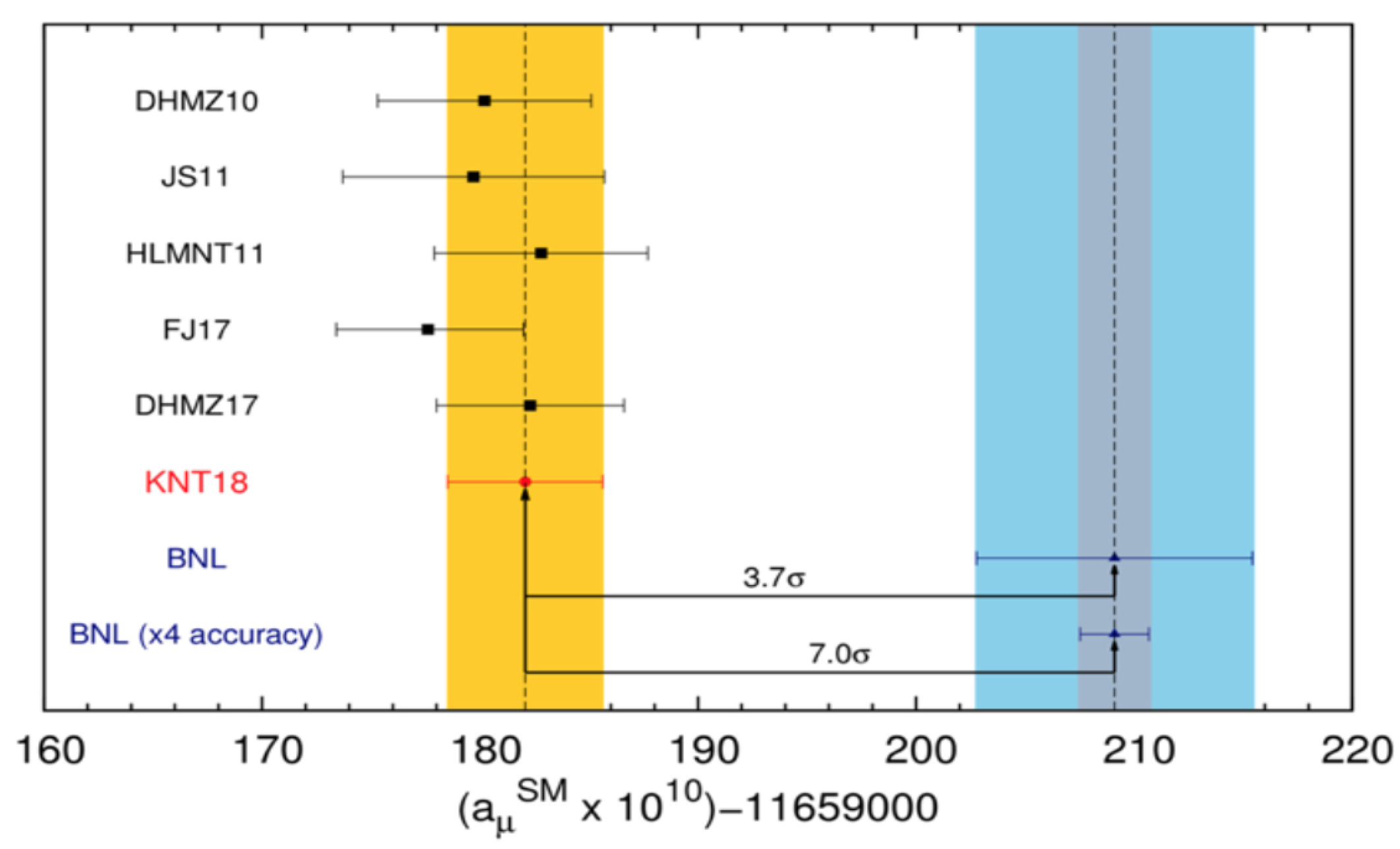
In Figure 2, the yellow band represents the prediction including uncertainty from the KNT18 calculation based on SM ( [3] with a precision of 420 ppb) and the blue band represents the latest experimental result from the previous Brookhaven E821 experiment combined with the experimental error ( [2]), which shows a difference of about 3.7 between theory and experiment. This could indicate several new physics models. These new models can be generally illustrated using a relation discussed in [4], in which new physics (N.P.) contributions scale as [5] , where M is the N.P. mass scale and C is the model’s coupling strength, related to any N.P. contributions to the muon mass, .
In the multi-TeV scale, a muon mass is corrected by radiative effects. Some new physics models may include Z, W, universal extra dimensions and littlest Higgs, which assume a typical weak-interaction coupling [5]. Other possibilities can represent unparticles, extra dimension models or SUSY (supersymmetry) with enhanced coupling [6]. The existence of dark photons or dark Z [7] from very weakly interacting (due to extremely small coupling of the muon with the dark photon) and very light particles corresponding to a narrow mass range of 10–100 MeV, can also be possible. Improved precision of measurement in to 140 parts per billion will continue to further constrain or validate the energy scale of the models, which is the goal of “The E989 Muon g–2 Experiment”. This requires 21 times more statistics than the previous Brookhaven E821 experiment and a threefold reduction of the systematic error.
2. The Measurement of Muon Anomalous Magnetic Moment: The Experiment
A polarized muon beam (from pion decay) having an energy of 3.09 GeV is injected (through the inflector shown in Figure 3) in a storage ring of uniform magnetic field of 1.45 T with a cyclotron frequency of . At the magic momentum of 3.09 GeV/c, the muon spin precession frequency (including the Larmor and Thomas precession) and are approximately given by,
Essentially the anomalous frequency , which is relative to , i.e., , is measured. From the above equations, this is given by,
In this experiment, the muon anomaly , is measured using the following expression [2],
where is the free proton precession frequency, and is the muon-to-proton magnetic moment ratio. The V-A nature of the muon decay makes it a self-analyzing process to find the muon anomalous precession frequency . The maximum energy decay positrons are emitted in a preferential direction with their momenta parallel to the muon spin. Some of these positrons modulate with a frequency of and this frequency can thus be extracted by counting the number of positrons above an energy threshold (optimized for the best sensitivity) as a function of time. Figure 3 (Right) shows the modulated counting rate of positrons observed in the 2001 E821 data. The value of is taken from muonic hyperfine splitting experiment, where it is measured at ≈26 ppb precision [8].
Figure 3 (Left) shows the schematic of the entire storage ring with the inflector, kickers (K1–K3), the quadrupoles (Q1–Q4), the straw trackers and the fiber harps. The details of each of these components are described in the subsequent sections. A positron/electron calorimeter is placed at a position indicated by the calorimeters in green numbers (1, 2, ..., 24). The decayed positrons are detected by the 24 calorimeters shown in Figure 3. The time spectrum of these positrons is given by,
from which is extracted. Here, is a threshold energy, is the asymmetry, is the number of events, is the phase term and is the muon lifetime. Care needs to be taken to account for the distortions in this spectrum due to pile up (i.e., overlapping events that originate from separate muon decays that are too close to each other in time and space to be resolved into individual pulses), gain instabilities, beam losses and other systematic effects.
2.1. The Preparation of the Muon Beam for Twenty-One Times the BNL Statistics
A statistical error improvement from 460 ppb to 100 ppb (≈21 times BNL) requires a better proton beam, and better proton and separation with an improved collection rate. This is accomplished by an 8 GeV proton produced in a booster which is then directed to a recycler ring (after several turns) further hitting an Inconel target to produce pions. Pions with an energy of 3.11 GeV are selected which decay to muons in a long decay channel before the beam (a mixture of protons, pions, muons, etc.) is injected into the delivery ring. This helps to produce polarized muons of energy 3.09 GeV from forward pion decays which provide better spatial separated from pions and background protons. Thus, using a delivery ring eliminates most of the background, gives a good spatial discrimination and reduces pion/proton flash. Finally, the muon bunches are transported to the muon storage ring in the Muon Campus 1 (MC1) experimental hall. An approximate run time of 18–24 months is required to acquire these statistics. To test all hardware equipment and installation of DAQ (Data acquisition) and DQM (Data Quality Management), along with other software, a month of the first engineering run in June 2017 took some commissioning data successfully. The first physics run (Run 1) from the end of March to 7 July 2018 took place and collected almost twice the raw positron data compared to the E821 experiment. A new Run 2 is scheduled to run from December 2018 to 15 July 2019, which is expected to collect ≈5–10 times more data than Run 1.
2.2. Muon Beam: Focusing in Storage Ring
As the muon beam enters the storage ring, it experiences a magnetic field from zero strength to the maximum value of 1.45 T, which causes it to deflect. The inflector magnet cancels these fringe field effects due to the main storage ring magnet, just before the beam enters the storage ring. It has a superconducting shield so that the field generated by the inflector current does not affect the uniform field of the storage ring. A new open-ended design inflector magnet is built for E989, which prevents scattering of muons at the exit of the inflector. This in turn will improve the muon storage efficiency. After exiting from the inflector, the muon beam is displaced radially outward by 77 mm from the ideal orbit. The three kickers direct the beam onto the ideal orbit with a pulsed vertical magnetic field which peaks at ≈250 G that corresponds to a kick of about ≈8 mrad [9]. Additionally, four electrostatic quadrupoles at 20.4 kV further enhances the radial focusing and enables the vertical focusing. They are made of aluminized mylar plates and have a coverage of about ≈43% of the circumference. The overall horizontal focusing is provided by the magnetic field. The muon beam is monitored using an Inflector Beam Monitoring System (IBMS1 and IBMS2). IBMS1 located just downstream of an initial time (T0) counter, consists of two planes (X and Y) of 16 cylindrical scintillating fibers of 0.5 mm diameter where the X (Y)-profile fiber pitch is 5.5 (2.7) mm. This is followed by IBMS2 located inside the beam injection pipe and has a similar design as IBMS1, except that the pitch is 3.25 mm for both planes. The two planes give the X and Y profile of the beam.
2.3. Further Improvements and Checks in Run 1
A few detectors were installed to improve beam monitoring during kicking and scrapping phases and to investigate the effect of coherent betatron oscillations. These were mainly the fiber harps and the straw trackers. The fiber harp system and the straw trackers are both used to determine the stored muon beam distribution. In Run 1, two fiber harps were used to study behavior of the muon beam flux and the horizontal and vertical oscillatory effects of the beam due to an electric field. These harps were installed at 180 and 270 near calorimeters 12 and 18, respectively, as shown in Figure 3. Two straw trackers were installed in the vicinity of calorimeters 16 and 22 respectively in Run 1, as shown in Figure 3.
2.3.1. Fiber Harps: Checking the Beam in Run 1
The fiber harps are strung with scintillating fibers and allow for a direct, but destructive, measurement of the distribution of stored muons and their associated beam dynamics parameters.
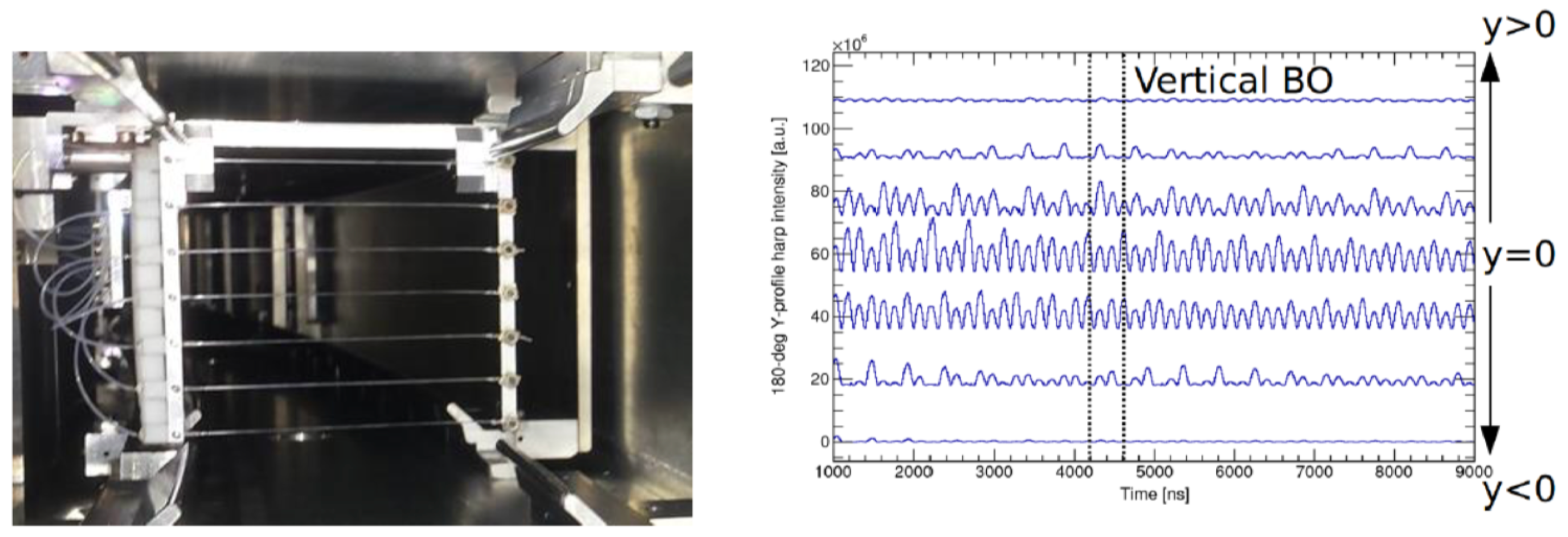
It consists of a “harp” of seven scintillating fibers of 0.5 mm diameter, each 90 mm long and separated from its neighbors by 13 mm [9]. Each scintillating fiber is further attached to a standard optical fiber as shown in the left image of Figure 4. A couple of such harps were used; one suspends the fibers vertically to measure x coordinates, and the other places the fibers horizontally to measure the y coordinates. Special fiber harp runs were occasionally taken in between data taking (not during the actual data runs as it is an obstacle to the beam). Figure 4 (Right) shows the horizontal measure in y of the beam profile. Maximum oscillations of the beam motion are in the center of the beam (around y = 0). This is due to the vertical component of the betatron oscillations.
2.3.2. Vacuum Straw Trackers
There are two In Vacuo straw tube trackers installed in the ring and each of them consist of 8 modules with 128 straws containing Argon–Ethane (50%) gas mixture, and having a resolution of 165 m. Each module has two planes of straws oriented at 7.5 with respect each other, so that both the horizontal and vertical coordinates of the trajectory can be determined. The straws are made of 15 m thick aluminized mylar foils with a gold-plated tungsten wire (d = 25 m) at the center.
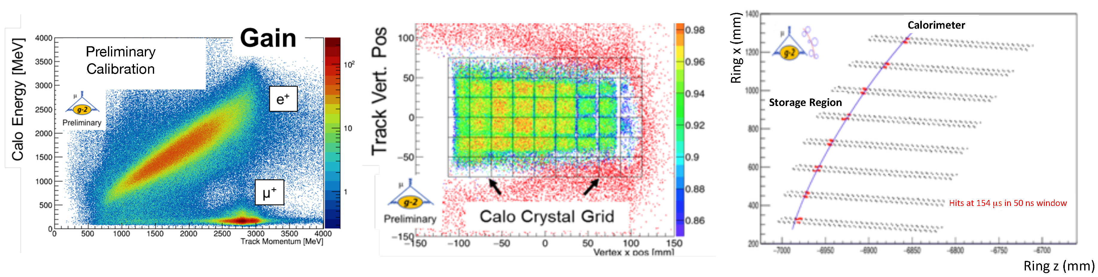
A forward extrapolation of the track to map with the front face of the calorimeter from the point of tangency of the muon track allows the determination of the beam profile distribution (Figure 5, Right). This, in turn, produces a good image of the positron distribution on the crystal grid of the calorimeters (Figure 5, Middle). The straw trackers in combination with the calorimeters show a good particle discrimination between positrons and muons based on the energy-momentum distribution (Figure 5, Left).
3. The Experiment: Systematic Improvements
To achieve our systematic uncertainty, it is essential to reduce the systematic uncertainties in the measurement of and , which requires further improvement in equipment and other procedures related the measurement of and . Systematics of 70 ppb on [9] is achieved by using an improved laser calibration, a segmented calorimeter, better collimator in the ring, and improved tracker. Systematics of 70 ppb on [9] is achieved by improving the uniformity and monitoring of the magnetic field, increasing accuracy of position determination of trolley, better temperature stability of the magnet, and providing active feedback to external fields [10]. This is discussed in detail in the subsequent subsections.
3.1. Systematic Improvements on
Table 1 shows the contribution to the systematics uncertainties of various factors on the measurement of and the proposed improvements. Here, the emphasizes is on the improvements in the calorimeters along with the laser monitoring system.
3.1.1. Calorimeters
The 24 calorimeters used to detect the decay positron spectrum are each made up of 54 (9 × 6) PbF crystals (for better time and space resolution, which improves pile up separation) with Silicon Photo Multipliers (better in enduring the magnetic field) and read out by custom 800 MSPS waveform digitizers.
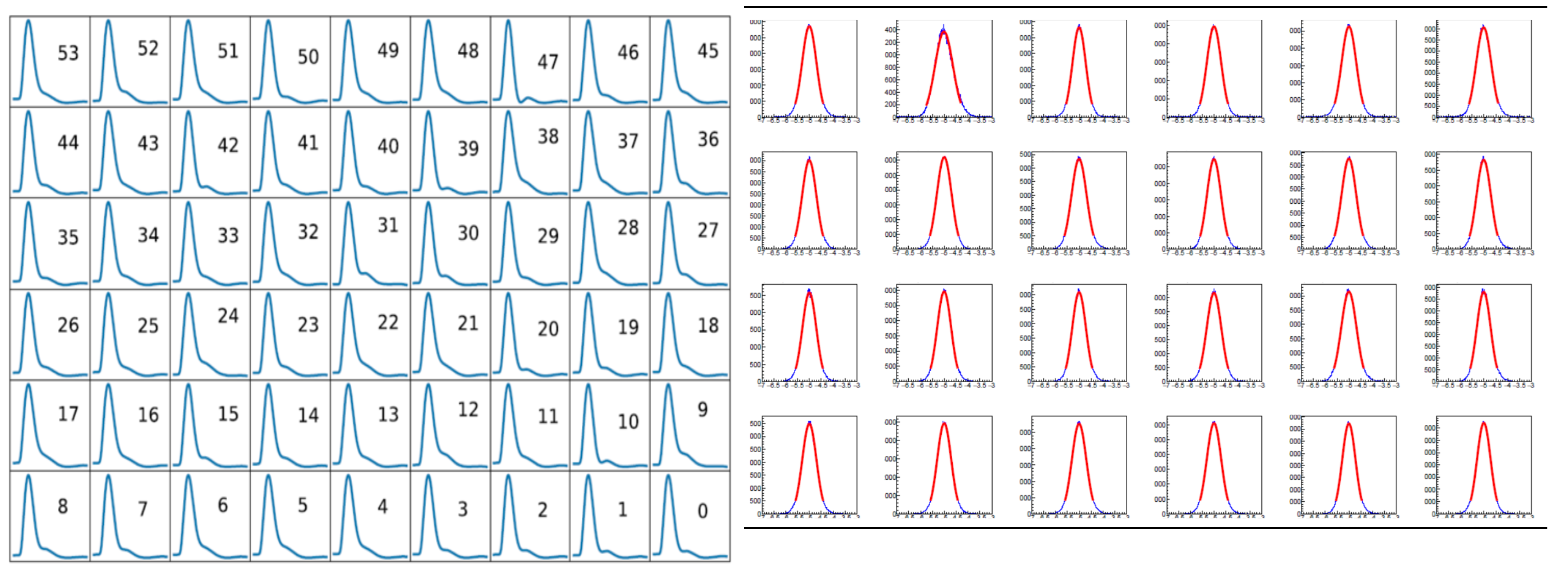
The pulses read by each crystal are reconstructed with a customized pulse shape fitting (called template fitting) to the actual pulses (as shown in Figure 6, Left). The time resolution of the crystals is 25 ps at 3 GeV providing a pile up separation of 4.5 ns.
3.1.2. Monitoring/Calibration of Calorimeter: Laser
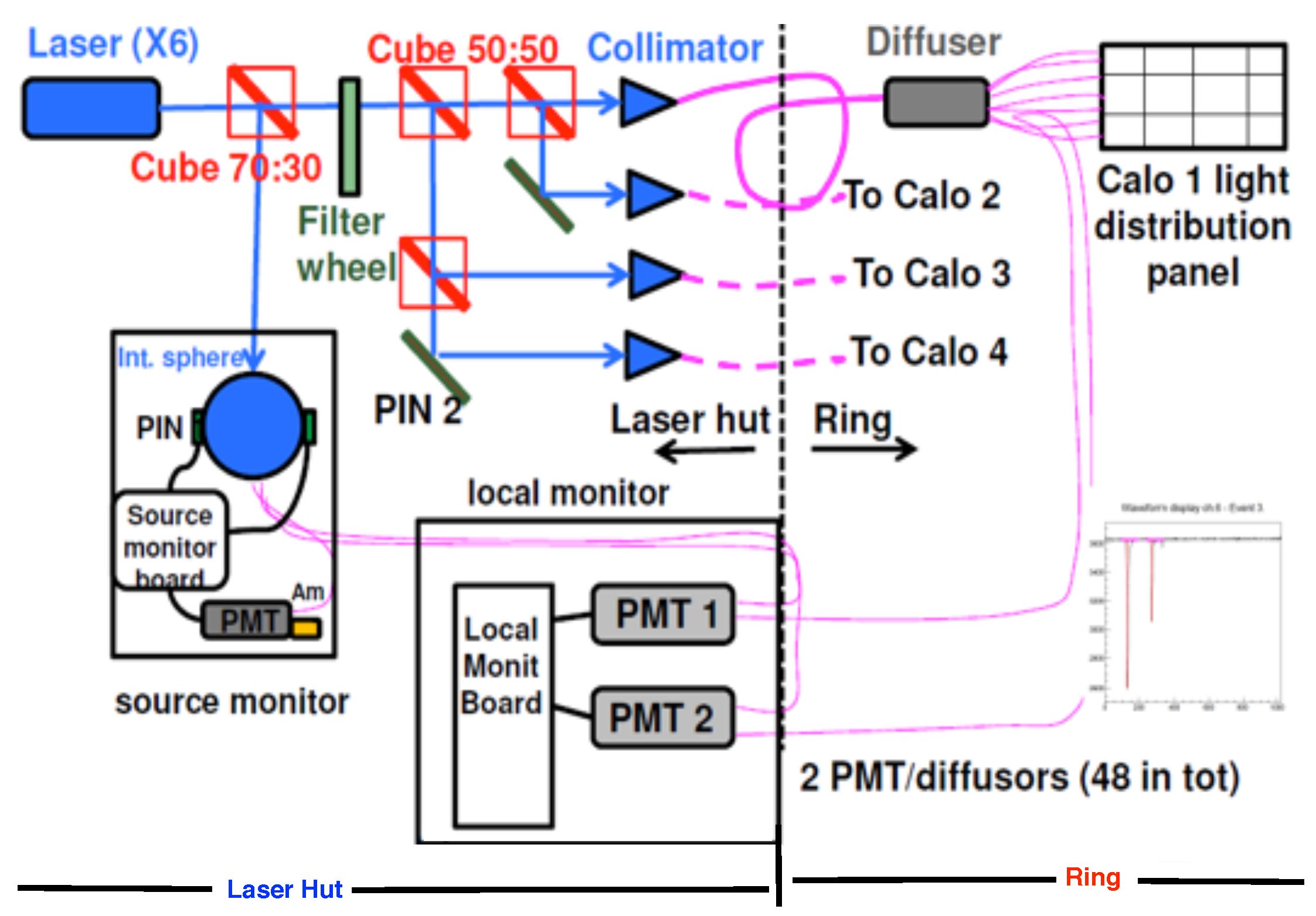
All 1296 channels of the calorimeters must be calibrated and monitored to keep uncertainties due to gain fluctuations at sub-per mil level in the time interval corresponding to one beam fill (700 s) and at the sub-percent level on longer time scales. This is done using the laser calibration system, as shown in Figure 7. Six laser heads (LDH-P-C-405M by PicoQuant) that provide up to 1 nJ of pulses 700 ps wide at a wavelength of 405 nm are used to calibrate all the calorimeters [11]. The light from each laser is divided with a ratio of 70:30 by a beam splitter. The 70% light is further divided into four equal parts and transported to four of the calorimeters in the ring using 25 m-long quartz optical fibers via a diffuser (to convert the Gaussian distribution of light intensity into a more uniform and flat distribution) and a fiber bundle.
This delivers light to each of the 54 PbF crystals with the fiber bundle attached to a Delrin panel embedded with optical prisms located in front of the calorimeter. A Source Monitor (SM) is used to measure pulse-by-pulse the intensity of the remaining 30% of the laser light.
The optical stability of this entire system is checked using 24 Local Monitor (LM). A mini-bundle fiber transmits light from the SM to the LM. Each LM consists of a PMT, which collects this light from the SM and is used as a reference signal. The light from the optical elements, the diffuser, and the 25 m quartz fiber (that transmits light to the calorimeter) is transmitted back to this PMT by using a quartz fiber. Thus, the 24 LMs are used to check the stability of the light distribution chain.
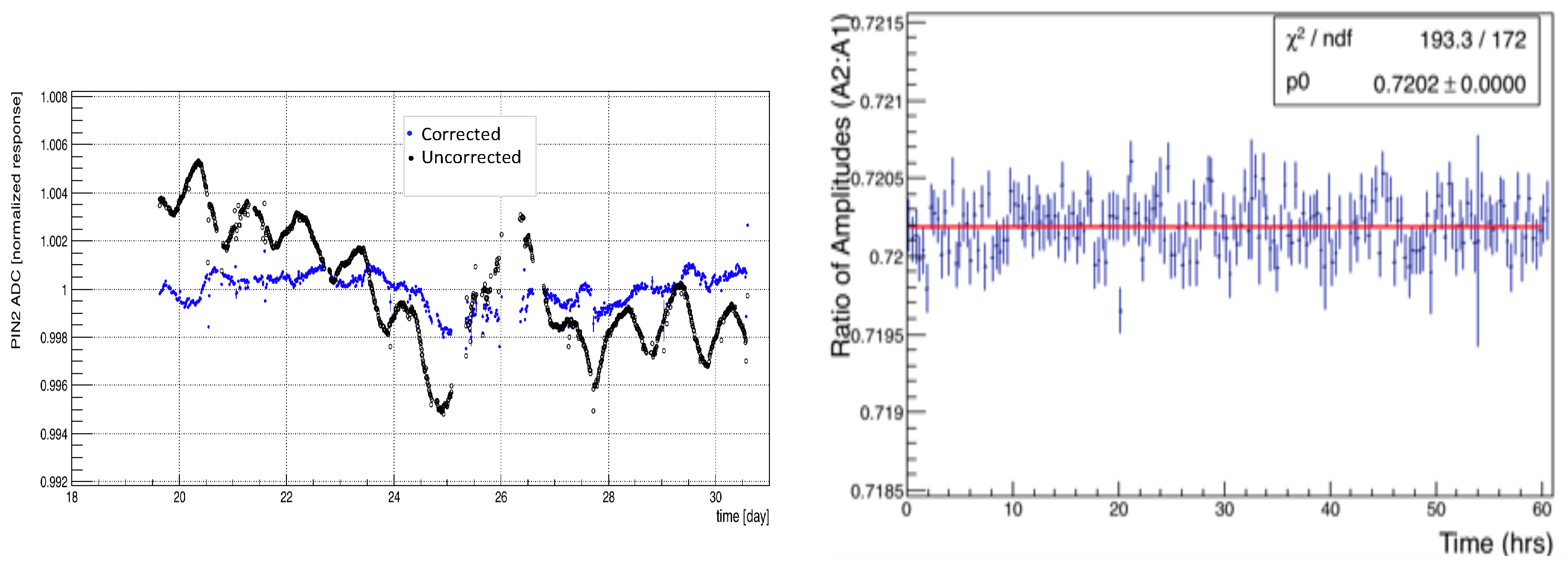
After applying temperature corrections, both the SM and the LM have fluctuations of the order of ≈10 (in a scale of hours), as shown in Figure 8. This is reasonably good for the desired precision of the experiment.
3.2. Systematic Improvements on
As mentioned above, the improvement of systematics on relies primarily on the uniformity and homogeneity of the magnetic field. It is briefly discussed how this was achieved in Run 1 and the other upgrades related to this.
Magnetic Field Homogeneity/Upgrade: Run 1
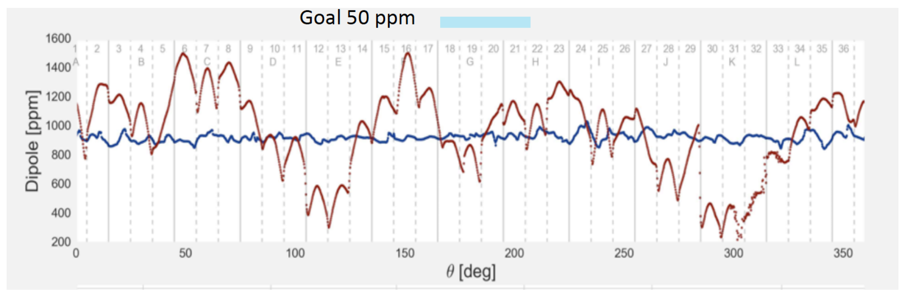
Iron shims were used to remove asymmetries due to quadrupoles and to eliminate fringe field and other stray field effects that distort the homogeneity of the main storage ring magnet. Top hats adjustments were used above the pole pieces (outside the yoke) to change the effective dipole moment. Usage of surface correction coils and iron foils made the field more uniform. Using iron lamination in Run 1 further increased the uniformity of the magnetic field to be within ±25 ppm of nominal value.
An absolute field calibration is essential for reducing the systematics on . A 1.45 T calibration magnet within a thermal enclosure (0.1 C) with additional probes and better electronics helped in achieving this. Trolley probe calibrations and trolley measurements of B (the central value of the magnetic field) need to be done with extreme care. Plunging probes were used to cross calibrate off-central probes with a better position accuracy. 378 fixed probes at 72 locations around the ring and more than 25 trolley calibration runs were used to improve the field mapping. The results of the improved stability of the magnetic field due to shimming, laminations, and calibration are shown in blue in Figure 9.
4. Run 1 Analysis Status
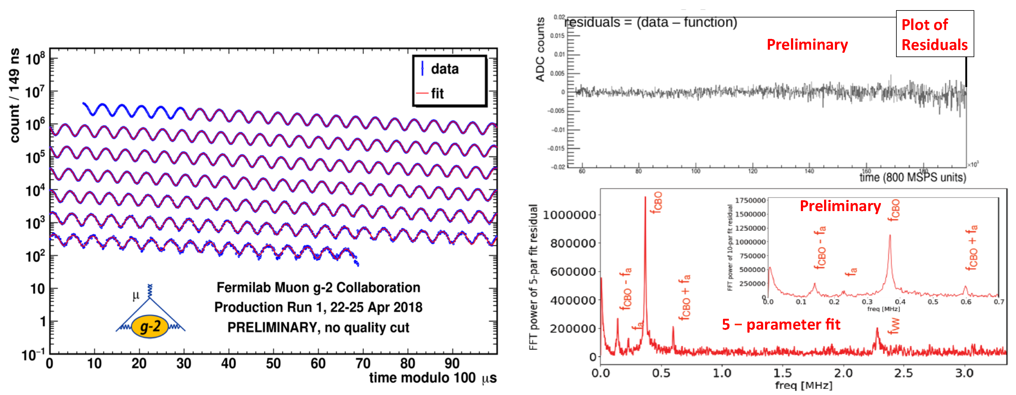
Several analysis techniques were developed and performed with the Run 1 dataset. All analysis methods utilized the event time and/or energy information reconstructed by the calorimeters with additional information from other detectors. One analysis method builds the events vs. time-in-fill histogram (so-called T-method) and then parameterizes the distributions with Equation (5) plus various systematic effects to extract . T-method selects events with reconstructed energy above a threshold energy (1.86 GeV) with the same weight. Pile-up correction is important for this method. From the previous simulation study [9] with T-method, a >95% polarization of the muon beam, an asymmetry of A = 0.38 and the number of events in the fit N = 1.6 × 10 yield a 100 ppb statistical uncertainty. A T-method fit to the positron time distribution is shown in Figure 10 (left). The fit residual together with its Fourier transform is in Figure 10 (right). The Fourier transform on the fit residual shows structures from CBO effects (), vertical oscillations () and muon losses (with other effects).
Another analysis method called Q(charge)-method digitizes the detector current vs. time distribution, which is proportional to the energy deposited in the calorimeters vs. time from the decayed positrons. All events are weighted inherently with energy and have a close to zero energy threshold (to reject background noises). The Q-method then parameterizes the energy distribution to extract . One advantage of this approach is that it does not require pile-up correction. There are also other analysis methods besides T- and Q-methods optimized in various ways and with different treatments of systematics and corrections. All methods serve as a cross check for each other and are combined afterwards to produce the final result.
A blind analysis was performed with both hardware offset (in clock frequency) and software offset (for each analysis method) to ensure that there is no bias in the final result.
5. Results and Conclusions
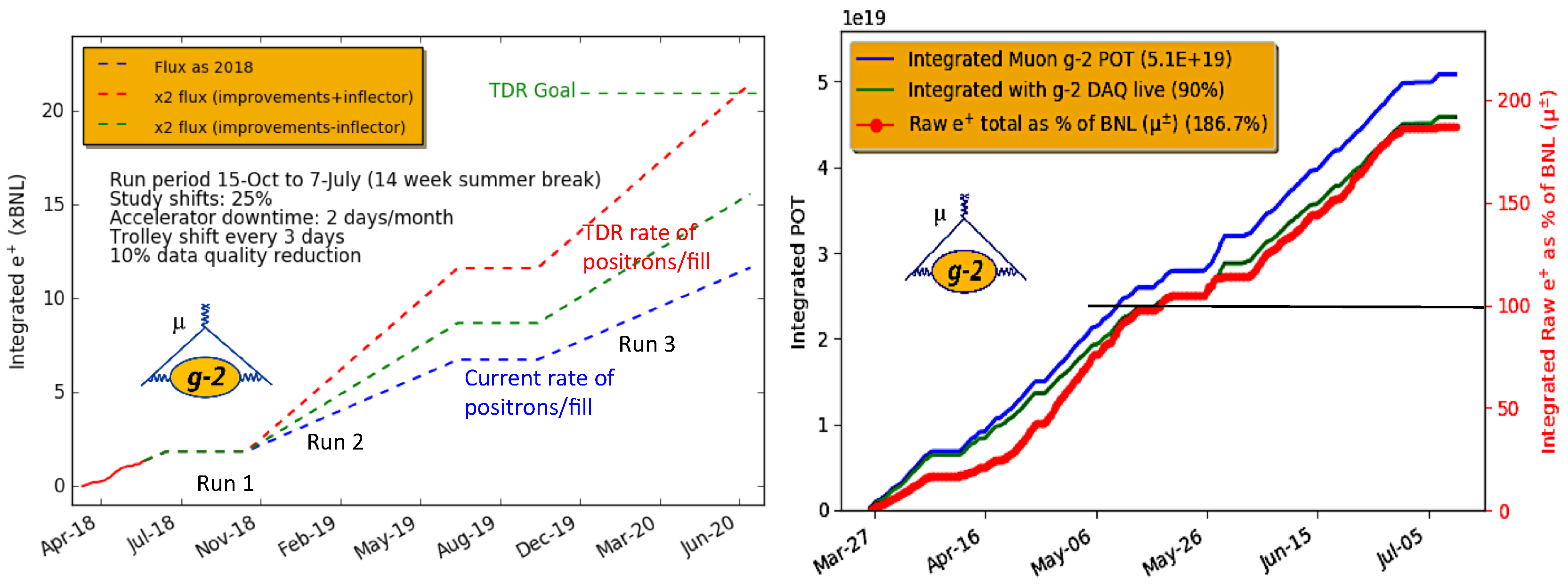
In Run 1, performance improvements in beam transportation, beam injection and detector systems were achieved. A significant improvement in systematics was also achieved, as discussed above. The data quality was good enough to find a signature of , but the current rate of positrons per fill is still below the expectation by a factor of two (compared to TDR Goal [9], as shown in Figure 11, Left).
Run 1, accumulated raw statistics ≈2 times the BNL experiment. After applying quality cuts for reconstruction of data, the accumulated statistics is about the same as that of the BNL experiment. A complete analysis of this data is expected to be done by the second half of 2019. The Run 1 result is expected to be at the same level of precision with the BNL experiment. In a few years, it is expected to measure the anomalous magnetic moment of the muon with the precision of 140 ppb. If the previously measured value of is confirmed, a seven-sigma discrepancy from SM will be evident, which would be a firm indication of new physics beyond the Standard Model.
Funding
This research was funded by Instituto Nazionale di Fisica Nucleare (Italy), by Fermi Research Alliance, LLC under Contract No. DE-AC02-07CH11359 with the United States Department of Energy, and by the EU Horizon 2020 Research and Innovation Program under the Marie Sklodowska-Curie Grant Agreements No. 690385 and No. 734303.
Conflicts of Interest
The author declares no conflict of interest.
References
- Schwinger, J. On quantum-electrodynamics and the magnetic moment of the electron. Phys. Rev. 1948, 73, 416–417. [Google Scholar] [CrossRef]
- Bennett, G.W.; Bousquet, B.; Brown, H.N.; Bunce, G.; Carey, R.M.; Cushman, P.; Danby, G.T.; Debevec, P.T.; Deile, M.; Deng, H.; et al. Final report of the E821 muon anomalous magnetic moment measurement at BNL. Phys. Rev. D 2006, 73, 072003. [Google Scholar] [CrossRef] [Green Version]
- Davier, M.; Hoecker, A.; Malaescu, B.; Zhang, Z. Reevaluation of the hadronic contributions to the muon g–2 and to α(MZ2). Eur. Phys. J. C 2011, 71, 1515. [Google Scholar] [CrossRef]
- Czarnecki, A.; Marciano, W.J. Muon anomalous magnetic moment: A harbinger for “new physics”. Phys. Rev. D 2001, 64, 013014. [Google Scholar] [CrossRef]
- Hertzog, D. Low-energy precision tests of the standard model: A snapshot. Ann. Phys. 2016, 528, 115–122. [Google Scholar] [CrossRef]
- Gorringe, T.P.; Hertzog, D.W. Precision Muon Physics. Prog. Part. Nucl. Phys. 2015, 84, 73–123. [Google Scholar] [CrossRef]
- Davoudiasl, H.; Lee, H.S.; Marciano, W.J. Dark side of Higgs diphoton decays and muon g–2. Phys. Rev. D 2012, 86, 095009. [Google Scholar] [CrossRef]
- Mohr, P.J.; Taylor, B.N.; Newell, D.B. CODATA recommended values of the fundamental physical constants: 2010. Rev. Mod. Phys. 2012, 84, 1527–1605. [Google Scholar] [CrossRef] [Green Version]
- Grange, J.; Guarino, V.; Winter, P.; Wood, K.; Zhao, H.; Carey, R.M.; Gastler, D.; Hazen, E.; Kinnaird, N.; Miller, J.P.; et al. [Muon g-2 Collaboration] Muon (g–2) Technical Design Report. arXiv, 2015; arXiv:1501.06858. [Google Scholar]
- Gohn, W. The muon g–2 experiment at Fermilab. arXiv, 2017; arXiv:1801.0008. [Google Scholar]
- Anastasi, A.; Basti, A.; Bedeschi, F.; Bartolini, M.; Cantatore, G.; Cauz, D.; Corradi, G.; Dabagov, S.; Di Sciascio, G.; Di Stefano, R.; et al. Electron beam test of key elements of the laser-based calibration system for the muon g–2 experiment. Nucl. Instrum. Meth. A 2017, 842, 86–91. [Google Scholar] [CrossRef]
Figure 1.
The SM contribution to from: (a) the tree-level diagram of the magnetic moment (where g = 2); and the subsequent corrections from: (b) QED; (c) EW loops; and (d) QCD.
Figure 1.
The SM contribution to from: (a) the tree-level diagram of the magnetic moment (where g = 2); and the subsequent corrections from: (b) QED; (c) EW loops; and (d) QCD.

Figure 2.
Comparison between theoretical and experimental results.

Figure 3.
(Left) The layout of the storage ring for the E989 experiment; and (Right) the modulated counting rate of the positron distribution of 2001 E821 data.
Figure 3.
(Left) The layout of the storage ring for the E989 experiment; and (Right) the modulated counting rate of the positron distribution of 2001 E821 data.

Figure 4.
(Left) The image of a fiber harp; and (Right) the beam profile in y direction measured by the fiber harp. Vertical BO means the vertical component of the betatron oscillations.
Figure 4.
(Left) The image of a fiber harp; and (Right) the beam profile in y direction measured by the fiber harp. Vertical BO means the vertical component of the betatron oscillations.

Figure 5.
(Left) Muon and positron discrimination from tracker data; (Middle) an imaging of the calorimeters from extrapolation of positron tracks from the tracker; and (Right) a positron hits in the tracker itself.
Figure 5.
(Left) Muon and positron discrimination from tracker data; (Middle) an imaging of the calorimeters from extrapolation of positron tracks from the tracker; and (Right) a positron hits in the tracker itself.

Figure 6.
(Left) The customized pulse shape fitting of all 54 crystals of a calorimeter; and (Right) the time resolution measurements fitted with a Gaussian function form for each calorimeter.
Figure 6.
(Left) The customized pulse shape fitting of all 54 crystals of a calorimeter; and (Right) the time resolution measurements fitted with a Gaussian function form for each calorimeter.

Figure 7.
A schematic showing the laser calibration system.

Figure 8.
The stabilities of the SM (Left) and LM (Right) after applying temperature corrections.

Figure 9.
Comparison of the magnetic field before (brown) and after (blue) shimming, laminations, calibration, etc. of the magnet.
Figure 9.
Comparison of the magnetic field before (brown) and after (blue) shimming, laminations, calibration, etc. of the magnet.

Figure 10.
A fit to the modulated positron distribution with time (Left); a plot of the fit residual (Top Right); and a Fourier transform of the fit residual (Bottom Right).
Figure 10.
A fit to the modulated positron distribution with time (Left); a plot of the fit residual (Top Right); and a Fourier transform of the fit residual (Bottom Right).

Figure 11.
(Left) The accumulated statistics of integrated positrons with future projections; and (Right) the accumulated statistics of POT (protons on target) in blue and the raw number of positrons in red for Run 1.
Figure 11.
(Left) The accumulated statistics of integrated positrons with future projections; and (Right) the accumulated statistics of POT (protons on target) in blue and the raw number of positrons in red for Run 1.


Table 1.
The table shows the systematics uncertainties of various factors on the measurement of .
| Category | E821 | E989 Improvement Plans (ppb) | Goal | Key Element (ppb) |
|---|---|---|---|---|
| Gain Changes | 120 | Better laser calibration | 20 | Laser |
| low-energy threshold | ||||
| Pile up | 80 | Low-energy samples recorded | ||
| Calorimeter segmentation | 40 | Calo | ||
| Lost Muons | 90 | Better collimator in ring | 20 | Calo |
| CBO | 70 | Higher n value (frequency) | <30 | Inflector + Kicker |
| Better match of beamline to ring | ||||
| E and pitch | 50 | Improved tracker | 30 | Tracker |
| Precise storage ring simulations |
© 2019 by the author. Licensee MDPI, Basel, Switzerland. This article is an open access article distributed under the terms and conditions of the Creative Commons Attribution (CC BY) license (http://creativecommons.org/licenses/by/4.0/).
Share and Cite
MDPI and ACS Style
Raha, N. The Current Status of the Fermilab Muon g–2 Experiment. Universe 2019, 5, 43. https://0-doi-org.brum.beds.ac.uk/10.3390/universe5020043
AMA Style
Raha N. The Current Status of the Fermilab Muon g–2 Experiment. Universe. 2019; 5(2):43. https://0-doi-org.brum.beds.ac.uk/10.3390/universe5020043
Chicago/Turabian StyleRaha, Nandita. 2019. "The Current Status of the Fermilab Muon g–2 Experiment" Universe 5, no. 2: 43. https://0-doi-org.brum.beds.ac.uk/10.3390/universe5020043
Note that from the first issue of 2016, this journal uses article numbers instead of page numbers. See further details here.