Mass Gap in Nonperturbative Quantization à La Heisenberg †


1
Institute of Experimental and Theoretical Physics, Al-Farabi Kazakh National University, Almaty 050040, Kazakhstan
2
Institute of Physicotechnical Problems and Material Science of the NAS of the Kyrgyz Republic, 265 a, Chui Street, Bishkek 720071, Kyrgyzstan
3
Institute of Systems Science, Durban University of Technology, P.O. Box 1334, Durban 4000, South Africa
*
Author to whom correspondence should be addressed.
†
This paper is based on the talk at the 7th International Conference on New Frontiers in Physics (ICNFP 2018), Crete, Greece, 4–12 July 2018.
‡
Current address: Department of Theoretical and Nuclear Physics, Al-Farabi Kazakh National University, Almaty 050040, Kazakhstan.
§
These authors contributed equally to this work.
Universe 2019, 5(2), 50; https://0-doi-org.brum.beds.ac.uk/10.3390/universe5020050
Submission received: 30 September 2018
/
Revised: 24 January 2019
/
Accepted: 28 January 2019
/
Published: 31 January 2019
(This article belongs to the Special Issue Selected Papers from the 7th International Conference on New Frontiers in Physics (ICNFP 2018))
Abstract
:The approximate method of solving nonperturbative Dyson-Schwinger equations by cutting off this infinite set of equations to three equations is considered. The gauge noninvariant decomposition of SU(3) degrees of freedom into SU(2) × U(1) and SU(3)/(SU(2) × U(1)) degrees of freedom is used. SU(2) × U(1) degrees of freedom have nonzero quantum average, and SU(3)/(SU(2) × U(1)) have zero quantum average. To close these equations, some approximations are employed. Regular spherically symmetric finite energy solutions of these equations are obtained. Energy spectrum of these solutions is studied. The presence of a mass gap is shown. The obtained solutions describe quasi-particles in a quark-gluon plasma.
1. Introduction
Quantum physical systems in quantum chromodynamics (QCD) have much more complicated structure than those in quantum electrodynamics (QED). In QCD, a quantum system may have a granular structure: hedgehogs/dyons with magnetic and electric fields appear as a result of quantum fluctuations. This is confirmed by lattice calculations, within which, using the maximal abelian projection, it was shown that in calculating the path integral, a considerable contribution comes from field distributions containing magnetic monopoles.
In the present work we study a microscopical structure of such fluctuations using the three-equation approximation for the nonperturbative set of Dyson-Schwinger equations. This approximation assumes noninvariant decomposition of SU(3) degrees of freedom into two groups. The first one contains SU(2) × U(1) components of a gauge field, the second one contains SU(3)/(SU(2) × U(1)) components of a gauge field.
The first group describes almost classical fields for which there exist the nonzero quantum average and quantum fluctuations :
Such a decomposition has been used in Ref. [1] to construct the Yang-Mills quantum-wave excitations propagating on the background of the classical homogeneous Yang-Mills condensate.
The fields belonging to the second group are purely quantum ones, since the quantum average
Below we will introduce the scalar field to describe the dispersion of these degrees of freedom. One can refer to the field as a condensate. In this connection, let us mention that in Ref. [2] a gauge-invariant description of a spatially homogeneous isotropic Yang-Mills condensate is discussed. Also, the paper [3] studies the gluon condensate relaxation phenomena using the nonlinear field equations for the gluonic condensate.
2. Nonperturbative Dyson-Schwinger Equations
Fundamental equations in nonperturbative quantization à la Heisenberg are the operator equations:
Here all physical quantities are operators of interacting fields which differ conceptually from operators of noninteracting fields used in perturbatively quantized theories like, for instance, QED; is the operator of the SU(3) gauge potential; is the corresponding operator of the field strength tensor; g is the coupling constant.
Apparently, these equations cannot be solved in the closed form. Thus, we consider the corresponding Dyson-Schwinger equations
Such infinite set of equations also seems to be extremely complicated to study. In this connection, the only possibility to solve this set of equations (at least approximately) appears to be the cutting off the infinite set of equations to a finite set of equations.
To do this, we use the following physical simplifications:
- We assume that in some physical situations all SU(3) degrees of freedom can be decomposed into two groups. In the first group, the gauge fields . In the second group, the gauge fields are pure quantum ones in the sense that .
- Decomposition for the 2-point Green function:
- Decomposition for the 4-point Green function:Thus, the field describes the dispersion of quantum degrees of freedom , and also the 4-point Green function for the operator .
- Decomposition for the 3-point Green function:The physical meaning of this approximation is that it is necessary to introduce some approximation for the interaction between the field and the spinor field describing quarks. The central idea of the approximation (12) is that the quantum average between the fields (at the points x and y) with zero average values (, see Equation (13)) is described by the product of the dispersion of the field , the correlation function from (14), and the dispersion of the field at the point x.
- For virtual quarks
- The correlation of virtual quarks at the points x and y isThus, the spinor and the Dirac conjugate spinor describe the dispersion of the spinor and the 3-point Green function .
- Interaction between the gauge field and the virtual quarks with nonzero quantum averages is described by the nonlinear interaction between their dispersions:
- We consider stationary systems only.
As a result, this leads to the following three equations (the three-equation approximation):
Here , , , and are quantum corrections coming from the dispersions of the operators from Equation (1) and from Equation (2). The appearance of these constants is a distinctive feature of any approach based on a truncation of an infinite set of equations to a finite one. In turbulence modeling, such constants are called the closure constants, see Ref. [4].
Equation (18) is obtained from Equation (5) for . Correspondingly, Equation (19) is obtained from Equation (5) for after averaging over all indices. Equation (20) is obtained from Equation (6). We note once more that Equations (18)–(20) are obtained using the above approximations.
Notice here one very important feature of the aforementioned constants: they have the dimensions which is absent in the initial Equations (3) and (4). As is known from QCD, there is a new parameter which is absent in the initial Equations (3) and (4). The parameters and are eigenvalues of the nonlinear eigenvalue problem, and that is why they can be rewritten in the form where this parameter is used:
Here the tilde means that these quantities are dimensionless. While solving the eigenvalue problem, one determines the quantities with tildes.
The physical meaning of these equations is as follows: the first Equation (18) describes a SU(2) massive gauge field from the subgroup SU(2) × U(1) ⊂ SU(3) interacting with the condensate of gauge fields from SU(3)/(SU(2) × U(1)) and with virtual quarks described by their dispersion ; the second Equation (19) describes an average dispersion of the coset fields from SU(3)/(SU(2) × U(1)) (the condensate) which interact with the field SU(2) × U(1) and with virtual quarks; the third Equation (20) refers to virtual quarks described by their dispersion and interacting with the fields and with the condensate .
3. Quasi-Particles in a Quark-Gluon Plasma
Lattice [5,6,7,8,9] and analytical investigations [10,11,12,13,14] indicate that a quark-gluon plasma contains various quasi-particles: monopoles, dyons, binary bound states (quark-quark (), quark-antiquark (), gluon-gluon (), quark-gluon (), etc.). Analytical calculations are phenomenological and they do not provide a macroscopic description of such objects. In Ref. [13], there is the following assessment of the state of this problem for a monopole: “…we do not have a microscopic description of these monopoles in terms of the gauge fields.”
The purpose of the present paper is to get a microscopic description of possible quasi-particles in a quark-gluon plasma based on some approximation for an infinite set of Dyson-Schwinger equations for nonperturbative Green functions. Consistent with this, below we describe possible types of quasi-particles in a quark-gluon plasma considered in the literature, and for some of them we present the resulting characteristics which can be compared with the characteristics obtained in our investigations.
3.1. Magnetic Monopoles
One of proofs of the existence of magnetic monopoles in a quark-gluon plasma is the calculation of the magnetic field flux created by such monopoles. Ref. [9] considers the behavior of the magnetic field flux as a function of distance from the center of a monopole,
where L is the effective length of the box and is the magnetic screening length. By going to the continuous limit , we get the following expression for the magnetic field flux:
In Section 5 the asymptotic expression (45) for the gauge field potential will be obtained, for which the corresponding radial component of color magnetic field is given by the expression
where the magnetic screening length is related to parameters of the system. Calculating this field flux through the sphere with the radius r, one can derive the expression (23).
In Ref. [13], the following indirect proof of the existence of monopoles is given: one calculates a semiclassical partition function that can be Poisson-rewritten into an identical “H” form. It is shown that it can be done for a pure gauge theory. After that point, it is argued that the resulting partition function can be interpreted as being generated by moving and rotating monopoles.
In Section 5 we obtain a solution that describes a “quantum monopole” with an exponentially decaying radial magnetic field that is needed to explain the lattice results.
3.2. Binary Bound States
Other possible quasi-particles in a quark-gluon plasma are binary bound states which describe states of two particles: , , , etc. In Ref. [10], it is noted that “…these bound states are very important for the thermodynamics of the QGP.” It is pointed out in that paper that to describe such objects approximately, one can use either the Klein-Gordon equation, or the Dirac equation, or the Proca equation. The essence of the suggested approach consists in that these equations are employed to describe two particles, interacting so that they create a coupled pair. To describe the coupling potential, one uses lattice calculations, based on which the analytical approximate expression for the potential is suggested.
One can fix the variables and in Equations (31)–(35): then the remaining Equations (34) and (35) will describe two quarks in a virtual state. This means that the quantum average of the corresponding spinor is zero,
but the dispersion of such a quantum state is nonzero. Physically, this means that the obtained solution describes a quantum object for which the average of field is zero but there exist quantum fluctuations whose dispersion differs from zero in some region. We assume that this solution microscopically and approximately describes the binary bound state where we neglect the distance between quarks and for which the orbital quantum number is zero.
4. Ansatz, Equations and Energy
Recall that we use Equations (18)–(20) to describe a microscopical structure of quantum excitations in a quark-gluon plasma, vacuum, etc.
We employ the following ansatz to obtain a hedgehog with color magnetic and electric fields:
Here is the completely antisymmetric Levi-Civita symbol; ; are the spacetime indices; the functions u and v depend on the radial coordinate r only; the ansatz (30) is taken from Refs. [15,16]. After substituting the Expressions (26)–(30) into Equations (12)–(14), we obtain the equations
In these equations, the following dimensionless variables are used: is the dimensionless coupling constant for the SU(3) gauge field; , where is a constant corresponding to the characteristic size of the system under consideration (one can show that this parameter is related to the constant ); , .
The total energy density of the system:
where the arbitrary constant corresponding to the energy density at infinity has been also introduced.
5. A Quantum Monopole Plus Virtual Quarks
For simplicity, consider a quantum monopole interacting with virtual quarks. In this case the set of equations is as follows:
These equations describe a system consisting of a quantum monopole, two virtual quarks, an extra color magnetic field created by them, and the condensate. These equations are solved numerically as a nonlinear eigenvalue problem where the eigenvalues are the parameters , and .
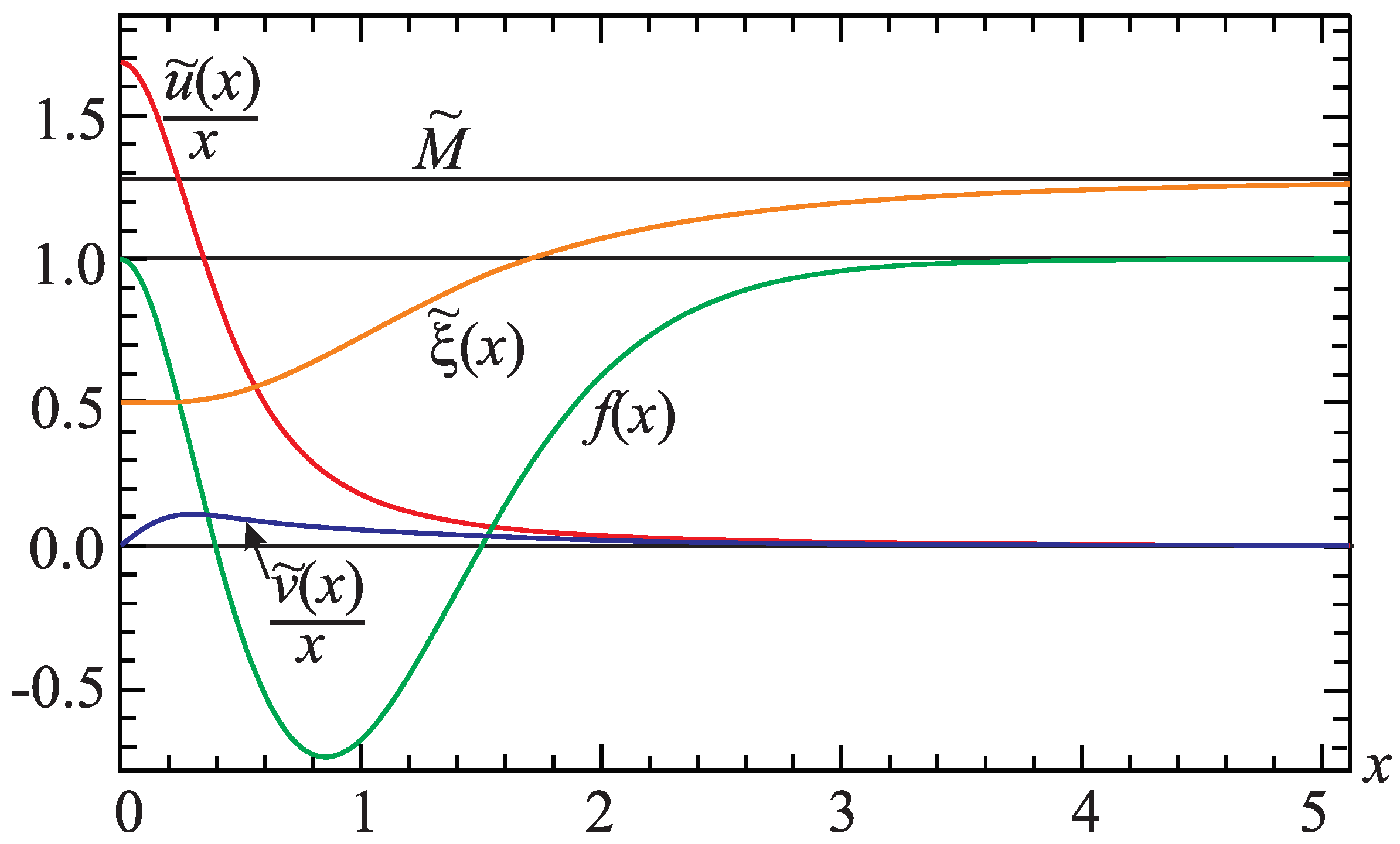
As , the solution of the above set of equations can be presented in the form of the following expansions:
Figure 1 shows the typical behavior of the solutions. Their asymptotic behavior as is
where , and are integration constants. The corresponding distributions of different components of the color magnetic field are shown in Figure 2.
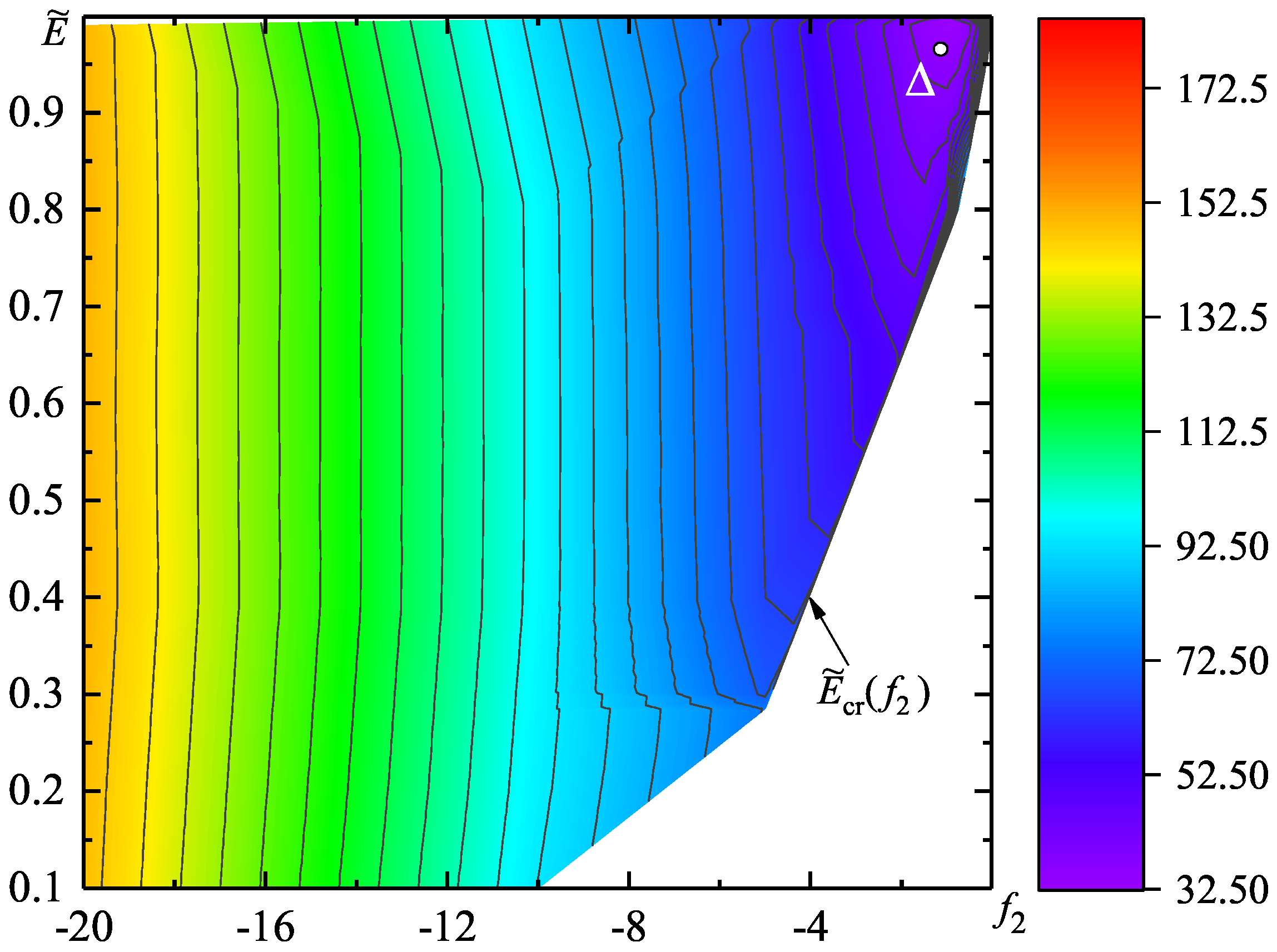
The dimensionless energy density of the system in question has the following form
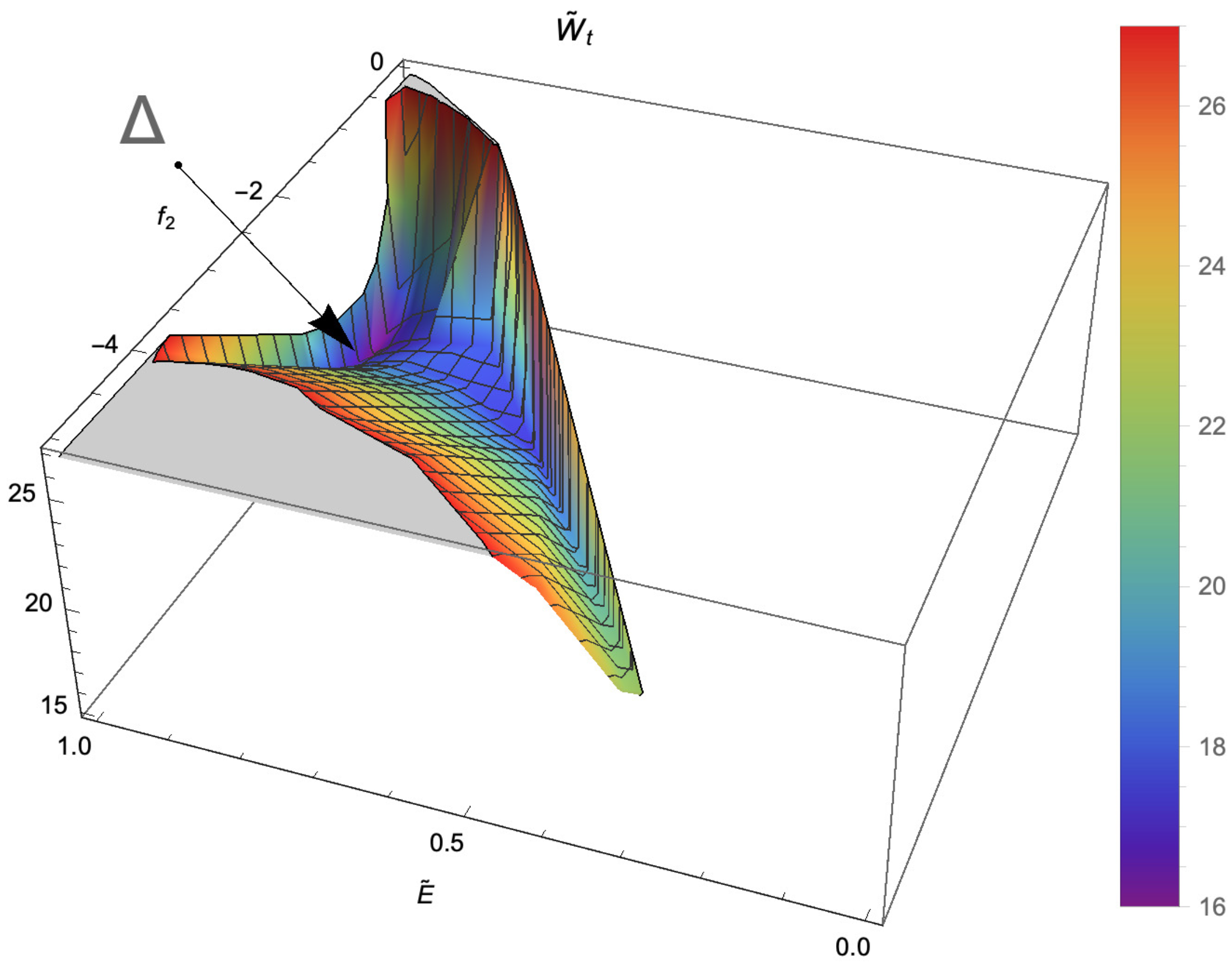
According to Equations (41)–(44), the total energy, as well as all functions, depends on the parameters and . To find the energy spectrum of the system “quantum monopole + virtual quarks”, we must obtain the dependence of the total energy (47) on these parameters. This dependence is shown in Figure 3 and Figure 4.
6. Physical Applications and Conclusions
In the present paper, we have employed the approximate gauge noninvariant approach to the set of Dyson-Schwinger equations to obtain an approximate microscopical structure of quantum fluctuations in a quark-gluon plasma, QCD vacuum and in other quantum systems within QCD. This means that we have verified the following model of quantum physical systems in chromodynamics: there is some condensate, on the background of which there are quantum fluctuations in the form of quantum monopoles/dyons filled with color magnetic (hedgehog) and electric (dyon) fields, and with virtual quarks (for which the quantum average is zero).
Thus, the following results have been obtained:
- Within the framework of the three-equation approximation, solutions describing virtual quarks and gauge fields in a bag have been found.
- It was shown that the bags are created due to the Meissner-like effect, when the coset condensate expels the gauge fields.
- For the quantum-monopole systems, it was shown that the color magnetic field decreases asymptotically.
- The nonlinear Dirac equation has been used as an approximate description of an infinite set of equations for all Green functions of the spinor equation.
We believe that the results obtained have the following physical meaning: the solutions obtained describe quasi-particles in a quark-gluon plasma. This means that in our approach, the quasi-particles are clumps consisting of quantum fluctuations of gluon and spinor fields and containing a radial magnetic field (a hedgehog).
It is interesting to note that in the 1950s the mass gap has in fact been found in Refs. [17,18] in solving the nonlinear Dirac equation. However, the authors did not use such term, but said of “the lightest stable particle”. Those papers were devoted to study of the nonlinear Dirac equation, and Heisenberg offered to use it as a fundamental equation in describing the properties of an electron.
Author Contributions
V.D.—conceptualization, V.F.—investigation.
Funding
This research was funded by Grant in Fundamental Research in Natural Sciences by the Ministry of Education and Science of the Republic of Kazakhstan grant number No. BR05236730.
Conflicts of Interest
The authors declare no conflict of interest.
References
- Prokhorov, G.; Pasechnik, R.; Vereshkov, G. Dynamics of wave fluctuations in the homogeneous Yang-Mills condensate. J. High Energy Phys. 2014, 2014, 3. [Google Scholar]
- Addazi, A.; Marcianò, A.; Pasechnik, R.; Prokhorov, G. Emergent Mirror Symmetry in Yang-Mills Vacua. arXiv, 2018; arXiv:1804.09826. [Google Scholar]
- Addazi, A.; Marcianò, A.; Pasechnik, R. Time-crystal ground state and production of gravitational waves from QCD phase transition. arXiv, 2018; arXiv:1812.07376. [Google Scholar]
- Wilcox, D.C. Turbulence Modeling for CFD; DCW Industries, Inc.: La Canada, CA, USA, 1994. [Google Scholar]
- Karsch, F.; Datta, S.; Laermann, E.; Petreczky, P.; Stickan, S.; Wetzorke, I. Hadron correlators, spectral functions and thermal dilepton rates from lattice QCD. Nucl. Phys. A 2003, 715, 701–704. [Google Scholar] [CrossRef] [Green Version]
- Karsch, F.; Laermann, E.; Peikert, A. The Pressure in two flavor, (2+1)-flavor and three flavor QCD. Phys. Lett. B 2000, 478, 447. [Google Scholar] [CrossRef]
- Laursen, M.L.; Schierholz, G. Evidence for Monopoles in the Quantized SU(2) Lattice Vacuum: A Study at Finite Temperature. Z. Phys. C 1988, 38, 501–509. [Google Scholar] [CrossRef]
- Koma, Y.; Koma, M.; Ilgenfritz, E.M.; Suzuki, T. A Detailed study of the Abelian projected SU(2) flux tube and its dual Ginzburg-Landau analysis. Phys. Rev. D 2003, 68, 114504–114521. [Google Scholar] [CrossRef]
- Bornyakov, V.G.; Ichie, H.; Koma, Y.; Mori, Y.; Nakamura, Y.; Pleiter, D.; Polikarpov, M.I.; Schierholz, G.; Streuer, T.; Stüben, H.; et al. Dynamics of monopoles and flux tubes in two flavor dynamical QCD. Phys. Rev. D 2004, 70, 074511. [Google Scholar] [CrossRef]
- Shuryak, E.V.; Zahed, I. Towards a theory of binary bound states in the quark gluon plasma. Phys. Rev. D 2004, 70, 054507. [Google Scholar] [CrossRef]
- Liao, J.; Shuryak, E. Strongly coupled plasma with electric and magnetic charges. Phys. Rev. C 2007, 75, 054907. [Google Scholar] [CrossRef]
- Ramamurti, A.; Shuryak, E. Effective Model of QCD Magnetic Monopoles From Numerical Study of One- and Two-Component Coulomb Quantum Bose Gases. Phys. Rev. D 2017, 95, 076019. [Google Scholar] [CrossRef]
- Ramamurti, A.; Shuryak, E.; Zahed, I. Are there monopoles in the quark-gluon plasma? Phys. Rev. D 2018, 97, 114028. [Google Scholar] [CrossRef]
- Shuryak, E. Are there flux tubes in quark-gluon plasma? arXiv, 2018; arXiv:1806.10487. [Google Scholar]
- Li, X.Z.; Wang, K.L.; Zhang, J.Z. Light Spinor Monopole. Nuovo Cim. A 1983, 75, 87–93. [Google Scholar]
- Wang, K.L.; Zhang, J.Z. The Problem of Existence for the Fermion-Dyon Self-Consistent Coupling System in a SU2 Gauge Model. Nuovo Cim. A 1985, 86, 32–40. [Google Scholar]
- Finkelstein, R.; LeLevier, R.; Ruderman, M. Nonlinear Spinor Fields. Phys. Rev. 1951, 83, 326–340. [Google Scholar] [CrossRef]
- Finkelstein, R.; Fronsdal, C.; Kaus, P. Nonlinear Spinor Field. Phys. Rev. 1956, 103, 1571–1580. [Google Scholar] [CrossRef]
Figure 1.
The graphs of the functions , and of the solution describing the spinball-plus-quantum-monopole system at , , , , , , , and . The corresponding eigenvalues are , , and .
Figure 1.
The graphs of the functions , and of the solution describing the spinball-plus-quantum-monopole system at , , , , , , , and . The corresponding eigenvalues are , , and .

Figure 2.
The profiles of the magnetic fields and for the spinball-plus-quantum- monopole configuration.
Figure 2.
The profiles of the magnetic fields and for the spinball-plus-quantum- monopole configuration.

Figure 3.
Contour plot of the total energy from Equation (47). shows the location of the mass gap in the plane.
Figure 3.
Contour plot of the total energy from Equation (47). shows the location of the mass gap in the plane.

Figure 4.
Three-dimensional plot for the dependence of the total energy (47) on the parameters and in the vicinity of the mass gap .
Figure 4.
Three-dimensional plot for the dependence of the total energy (47) on the parameters and in the vicinity of the mass gap .

© 2019 by the authors. Licensee MDPI, Basel, Switzerland. This article is an open access article distributed under the terms and conditions of the Creative Commons Attribution (CC BY) license (http://creativecommons.org/licenses/by/4.0/).
Share and Cite
MDPI and ACS Style
Dzhunushaliev, V.; Folomeev, V. Mass Gap in Nonperturbative Quantization à La Heisenberg. Universe 2019, 5, 50. https://0-doi-org.brum.beds.ac.uk/10.3390/universe5020050
AMA Style
Dzhunushaliev V, Folomeev V. Mass Gap in Nonperturbative Quantization à La Heisenberg. Universe. 2019; 5(2):50. https://0-doi-org.brum.beds.ac.uk/10.3390/universe5020050
Chicago/Turabian StyleDzhunushaliev, Vladimir, and Vladimir Folomeev. 2019. "Mass Gap in Nonperturbative Quantization à La Heisenberg" Universe 5, no. 2: 50. https://0-doi-org.brum.beds.ac.uk/10.3390/universe5020050
Note that from the first issue of 2016, this journal uses article numbers instead of page numbers. See further details here.