Zeta Functions and the Cosmos—A Basic Brief Review


1
Consejo Superior de Investigaciones Científicas, ICE/CSIC-IEEC, Campus UAB, Carrer de Can Magrans s/n, Bellaterra, 08193 Barcelona, Spain
2
International Laboratory for Theoretical Cosmology, Tomsk State University of Control Systems and Radioelectronics (TUSUR), 634050 Tomsk, Russia
Universe 2021, 7(1), 5; https://0-doi-org.brum.beds.ac.uk/10.3390/universe7010005
Submission received: 7 December 2020
/
Revised: 22 December 2020
/
Accepted: 24 December 2020
/
Published: 30 December 2020
(This article belongs to the Special Issue The Casimir Effect: From a Laboratory Table to the Universe)
Abstract
:This is a very basic and pedagogical review of the concepts of zeta function and of the associated zeta regularization method, starting from the notions of harmonic series and of divergent sums in general. By way of very simple examples, it is shown how these powerful methods are used for the regularization of physical quantities, such as quantum vacuum fluctuations in various contexts. In special, in Casimir effect setups, with a note on the dynamical Casimir effect, and mainly concerning its application in quantum theories in curved spaces, subsequently used in gravity theories and cosmology. The second part of this work starts with an essential introduction to large scale cosmology, in search of the observational foundations of the Friedmann-Lemaître-Robertson-Walker (FLRW) model, and the cosmological constant issue, with the very hard problems associated with it. In short, a concise summary of all these interrelated subjects and applications, involving zeta functions and the cosmos, and an updated list of the pioneering and more influential works (according to Google Scholar citation counts) published on all these matters to date, are provided.
1. Introduction
The unreasonable effectiveness of mathematics in the natural sciences, as Eugene Wigner put it, is an old and, as of now, still intriguing question [1]. For, in some way, it can be traced back at least to the Pythagorean school (ca. 550 BC, “all things are numbers”), and quite possibly to the Sumerian and Babylonian civilizations, and even perhaps to some more ancient ones. Much more recently, Immanuel Kant wrote that “the eternal mystery of the world is its comprehensibility” and also Albert Einstein, in his essay from 1936, entitled “Physics and Reality", defended exactly the same concept and with almost the same words.1 Mathematical simplicity and beauty are commonly considered to be reliable criteria when choosing among different possible theories. However, scientist do not use now words such as ‘comprehend’ or ‘understand’ anymore, at least so often. They have been nowadays replaced by ‘describe’ or ‘model’, in reference to the theories of nature. An example I particularly like is the following. Let us consider Newton’s law that affirms that two bodies will always attract each other with a force proportional to the product of their masses and inversely proportional to the square of the distance that separates them. This law is very simple and absolutely universal, valid in an enormously wide range of scales, from those of our normal life to the ones of the solar system and even to much larger scales in the cosmos. But, does this mean that we actually understand this law? Not at all; it only means in fact that we can describe this attraction law in an extremely simple, accurate, and universal way. Needless to say, the main point risen before still remains: why on Earth are we able to describe the cosmos in terms of so simple equations, just by using our little minds?
The regularization methods and procedures employed in quantum field theory (QFT), and which we will consider in this paper, constitute clear examples of this unreasonable effectiveness of mathematics. Analytic continuation on the complex plane is fundamental in many of these methods, namely in dimensional, heat-kernel, and zeta-function regularization. After some weird mathematical manipulations, we eventually obtain physically reasonable, experimentally measurable, and even extremely precise results. If not unreasonable, this is at least quite mysterious. Several important physicist, including Albert Einstein and Paul Dirac, the last one a real genius when working in the interface of mathematics and physics, were of the opinion that all these procedures were just unjustified tricks, only admissible for a while, until the real physical theory would finally be discovered. But it turned out that, in the end, these methods could be rigorously justified (at least mathematically) and they were even blessed with the Physics Nobel Prize in several occasions. Although one can argue that this actually happened because of the many and very precise experimental results obtained with those methods; namely, for their effectiveness, rather than because they were reasonable.
We face up an example of this situation when we calculate the very simple case corresponding to the vacuum to vacuum transition, or zero point energy (or, also, the related Casimir energy [2]) of a quantum operator, H, whose spectral values are , namely
Note this is a simplified notation, since the ‘sum’ over n may actually include a number of different, continuous and discrete indexes. This sum will be convergent in very special cases, only. Generically one will have to deal with a divergent multiple series or integral (or both), which needs to be regularized by some mathematical means. And the final result, even if it is finite, must be interpreted and given a physical sense.
Interestingly enough, series of this same form appear in very different contexts, to wit in music. There, the corresponding eigenvalues are very simple, namely natural numbers and, as eigenvalues of a related physical system, correspond to the standard case of an harmonic oscillator. Actually, in music the harmonic series is defined to be a sequence of sounds, corresponding to pure tones, which in physical terms are sine waves, where each sound has a frequency that is an integer multiple of the lowest frequency of all them, a base note called a fundamental.
Musical instruments often contain an acoustic resonator, most commonly a string or an air column, oscillating simultaneously in various modes. At the frequency corresponding to each mode, the waves travel in both directions along the string or air column, depending on the musical instrument. And they reinforce or cancel each other out eventually forming standing waves. These waves propagate through the air, so that audible sound waves reach us, coming from the instrument. Owing to the typical distance of the resonances, the frequencies are generically limited to multiple integers, called harmonics, of the lowest frequency. This sequence of multiples constitute the harmonic series.
One usually perceives the musical tone of a note as the lowest partial present (the fundamental frequency). This is produced by vibrations along the whole length of the string or air column; but it can be also a higher harmonic chosen by the player. The musical timbre of a constant tone essentially comes from the relative strength of each harmonic. Properly combined, harmonic components can build sublime music and through it we can experience an indescribable, unparalleled pleasure. Without doubt, one of the greatest experiences we can possibly enjoy with our senses.
Back to our mathematics, it is now not surprising that the harmonic mathematical series is defined as follows:
It corresponds to the sum of all the wavelengths of the successive notes of the vibrating string, which are, as we have already advanced, 1/2, 1/3, 1/4, and so forth, of the fundamental wavelength. Each term in the series, after the first one, is the harmonic mean of its neighboring terms. Mathematically, this is a divergent series, since, for any given value we may fix, a sufficient number of its terms will add up to a value that is larger than the fixed one. The harmonic series is closely linked to the most important and mysterious function of all of mathematics, namely the zeta function, .
Leonard Euler (1707-1783), who was the mathematician who introduced it, firmly believed that “One could assign a number to any series” [3,4]; that is, of course, in a mathematically consistent way, and also useful for practical purposes. Such statement was meant to be also true, of course, for divergent series. Euler was not able to demonstrate this statement rigorously, but he constructed a procedure (now called Euler’s criterion) designed to obtain the corresponding ‘sum’ for different families of series, which in principle were divergent. However, some other great mathematicians did not agree with him at all, as Abel, for instance, who used to say the following: “Divergent series are the invention of the devil, and it is a shame to base on them any demonstration whatsoever” [5]. The also famous mathematician G.H. Hardy wrote what is now a classic book on this subject, Divergent series [6], a very recommendable reference.
In the present paper, a very elementary, highly pedagogical review of the zeta function method will be given, stressing the basic concepts and the history of this procedure, always with the idea of complementing other works were much more rigorous presentations have been given. It will be then explained how the method can be used for the regularization of physical quantities, such as quantum vacuum fluctuations in several contexts, with the use of very basic examples. In special, in Casimir effect setups and mainly concerning its application in quantum theories in curved spaces, together with its different uses in gravity theories and cosmology. A summary of all these concepts and applications, and an updated perspective of the whole development, will be provided in the different sections, as follows. Section 2 is devoted to very basic issues on the zeta function. Section 3 deals with the concepts of a divergent series and of zeta regularization. Section 4 contains a discussion of the interplay between the concepts of vacuum energy and the cosmological constant, from the modern perspective of quantum physics. The section starts with a review of the pioneering observations that led to the proof that the universe is, to very good precision, homogeneous and isotropic; what eventually led to the formulation of the now standard Friedmann-Lemaître-Robertson-Walker (FLRW) model. Section 5 contains a very short introduction to zeta-function regularization in curved spacetime. In Section 6, the quantum vacuum interpretation of (or contribution to) the cosmological constant is used to address the cosmological constant problem. Examples of the use of the zeta regularization procedure in cosmology are there discussed, including also a short incursion in the dynamical Casimir effect. Finally, the closing section, Section 7, is devoted to an overall summary and conclusions.
2. Basics on Zeta Functions
Regularization and renormalization procedures, which are the names of the methods physicist use to fulfill Euler’s dream in Quantum Field Theory (QFT), are fundamental in contemporary Physics [7]. They have proven to be crucial in order to give a sense to all these theories. There are different techniques for implementing these procedures in practice. The problem is the following. When one perturbatively computes say, a correlation function for some QFT, one obtains a formal power series in the bare parameters that characterize the theory. This formal power series is generally divergent, or sometimes asymptotic. In order to be able to manipulate it by using mathematical techniques, the first step is always to produce from it an expression in terms of dimensionless quantities (which replace the dimensional quantities one always starts with). For this purpose, the series (or integrals) one started from are made to depend on some parameter, usually denoted as (a dimensionfull scale), and are rendered finite provided does not take on a certain limiting value, corresponding to the physical regime (like the UV) that led to the original divergence. After regularization, we then renormalize and find (in good, so-called renormalizable theories) that drops out of the physical results, which are finally independent of it and of the regularization procedure used. Actually, there is no mathematically precise, generally accepted definition of the term “regularization procedure” in perturbative quantum field theory. Instead, there are various regularization schemes, all of them with some advantages and disadvantages. Among them, we can count the dimensional [8], Pauli–Villars [9], lattice [10], cut-off [11,12,13,14], zeta function, causal [15], and Hadamard regularization [16,17]. This is, I repeat, a very extensive and fruitful field. It is key for the definition itself of a QFT. I cannot go into any detail of the definitions and main characteristics of the different methods but the interested reader is addressed to the selected references I have given.
Among all these methods, zeta function regularization is particularly elegant and efficient, at least from a mathematical viewpoint. It is in fact the standard method used by mathematicians in operator theories, in the formulation, for example, of the famous Atiyah-Singer theorem [18,19,20,21,22,23]. In physics, this constitutes a very important method to obtain, for instance, the energy of the vacuum state for a quantum physical system. This energy could, very possibly, provide a contribution to the universal force (the dark energy), which is responsible for the presently observed acceleration of the cosmic expansion.
The procedure of zeta function regularization is very well suited for calculating the fluctuations of the vacuum energy corresponding to the quantum fields pervading the universe; in particular, their possible contribution to the cosmological constant (cc). A calculation of these fields’ contribution, in order of magnitude, by employing a cut-off of the Planck length order, yields a value that, already at this level, differs in many orders from the one coming from the astronomical results. This is called the cosmological constant problem. Such an issue, which implies at first sight an impossible fine tuning, is not easy to solve, as widely known. Thus, several authors still start by first trying to solve the old problem; namely they intend to prove that the ‘naked’ value of the cc could still be zero, in the hope that there might appear some non-vanishing additional perturbations thereof, which would eventually lead to the (small) observed result.
Some time ago, we also worked on this problem in a quite analogous way, and considered the additional contributions to the cc, which could possibly appear when taking into account the effects of a non-trivial topology for the space and also depending on the boundary conditions, which usually are imposed on braneworld models and some other ones that are discussed in the literature. This would be, more specifically, a sort of Casimir contribution. We still expect that it might play an important role in cosmology, and it will be reviewed here. If we could prove that, for some reason, the (let us call it bulk or naked) value of the cosmological constant is actually zero (there are some results that indicate this could be true [24,25,26,27]), in this case we would just be left with such small additional contribution, which appears from the non-trivial topology and/or the boundary conditions. If the value that we obtain, coming from these perturbations, would have at least the correct order of magnitude, as compared with the astronomical data (and the right sign too, what is also quite an issue), then we would be on the right track to solve this fundamental problem. The last part of the argument was shown to be indeed realizable, at least in a crude approach, in some simple examples that capture the essence of the procedure. A further step in this direction is to introduce into the play the so-called dynamical Casimir effect (or sometimes Davies-Fulling theory). It is still not yet completely clear how this effect should be taken into account in cosmology, but it is a fact that the boundaries of (at least the visible) universe are expanding with it and this naturally calls for that effect. Some ideas concerning the renormalization at laboratory scales of such effect have been already pursued, with quite hopeful results. We will briefly discuss those issues later.
At the one-loop level the zeta function method is at its best. At such level, this method is defined rigorously, and many QFT calculations there are reduced, basically and from a mathematical perspective, to calculate the determinants of elliptic pseudodifferential operators (DOs) [28]. It should not be surprising, therefore, that the most common definition of determinant for dealing with those operators is the one that emerges from the zeta function corresponding to the operator, as explained in Ref. [29,30,31].
A crucial point is now the following. The zeta function regularization method relies, for its practical application [32,33], on the existence of explicit and particularly simple expressions, which provide the analytic continuation of the series defining the zeta function, , on the right of the abscissa of convergence, Re , where the function is well defined as an absolutely convergent series, to the other side of the complex plane [29,30,31,34,35,36]. Aside from the reflection formula of the corresponding zeta function in each case, which is known to exist always, there are also some other fundamental expressions that are much more useful in practice. We are talking of Poisson’s and Plana’s summation formulas, the Jacobi theta function identity, and the Chowla-Selberg series formula, among other. The problem is now that these formulas are usually restricted to rather concrete zeta functions, and also, that the derivation of the explicit, final expressions is very often rather difficult, and they are not available in the literature, in some cases. For instance, until a few years ago, the Chowla-Selberg (CS) series formula was only known explicitly for the original case of the homogeneous Epstein zeta function in two dimensions, but not in inhomogeneous cases and neither in higher dimensions. Moreover, all such expressions rely on the much important detail that the running index for the sum must go over a whole lattice, for example, extending from to , every single index, in say or . The formulas are no more valid in the case of truncated sums—which are precisely the ones that more often appear in physics. In those case one can only get much more involved, asymptotic expressions [34,35].
A basic and very important property common to any zeta function is the so-called reflection formula or functional equation. It has the following form, in the case of the Riemann zeta:
In general, for an arbitrary zeta function, , let us write it as: This formula provides the explicit expression of the analytic continuation, in the way we have explained. In very simple situations, this is practically all the story, and the short description of the zeta function method could actually be finished here. At least in principle, as we will now discuss. The problem being namely that the expression obtained by analytic continuation is also a series, and will again converge very slowly (power slow convergence, in fact, the same type displayed by the original series on the right of the complex plane) [37]. Neither the original series expression for the zeta function nor the analytically continued one on the lhs of the complex plane are of much use for dealing with values of the variable that are close to the abscissa of convergence. As discussed, for example, in Ref. [37] in much detail, one has to add an incredible number of terms of the zeta function series in order to get a value that makes sense as a reliable approximation, when approaching this abscissa. That is why the following addendum to the short story is so important.
For the case of the Epstein zeta function, an exceptional formula was found by S. Chowla and A. Selberg (details on it will be given later) in the two-dimensional case [38], which exhibits exponentially fast convergence everywhere on the complex plane (not only on the extended domain). These authors were very happy to have obtained such formula, as we can see if we read their original articles. In Ref. [39], a first attempt was carried out by the author of the present paper to try to generalize this formula to the case of non-homogeneous zeta functions, since this is crucial for physical applications, see Ref. [40]. This extension was still in dimension two, what was then believed to be a constraint of the CS expression (see, e.g., Ref. [41]). Some time later, extensions to an arbitrary number of dimensions [42,43], in the cases of a quadratic, homogeneous form and of a non-homogeneous form (the quadratic one, plus an affine form) could be also constructed. In any case, some of these new expressions (and in particular those for to the zero-mass case, which correspond precisely to the original CS formula) turned out to be not explicit, but just recurrent expressions. The solution to the problem had the form of a quite involved recurrence—this was also probably the reason that the CS formula could not be generalized so easily to Epstein zeta functions in higher dimensions. Finally, at a second stage, we were able to explicitly solve the recurrence [44] and, in this way, explicit formulas extending the CS series formula could be finally obtained, for the first time. I should note here that all this work was carried out by the author of the present paper, which he is actually very proud of.
Let us conclude this section by recalling that, on top of the quadratic case, directly corresponding to the Epstein zeta function and its generalization, another very important one is the linear case, which in spite of its simple aspect is also very difficult, too. It is equally important because it has a lot of applications in physics, where it corresponds to a system of harmonic oscillators or of a multidimensional oscillator. The most general zeta function corresponding to the linear case goes under the name of Barnes zeta function. Once more, we also miss, in this case, many explicit formulas corresponding to the most general expression, in particular for its derivatives.
3. On Divergent Series and Zeta Regularization
After this very general overview of the most common zeta functions, let us start again from the beginning; this time from the viewpoint of the already announced divergent series. As is usual in modern presentations of mathematical theories, and following Hardy [6], one usually starts the discussion of divergent series by listing some reasonable axioms to be fulfilled, in order to give sense to their sum; like the following ones:
- If , then .
- If , and , then.
- If , then .
Let us now consider a couple of very simple examples.
- From axiom 3, for the series , we obtain , and from there . This seems reasonable, because the partial sums of this series oscillate between 0 and 1, and 1/2 is the middle value.
- From axiom 2, we see that for , when we subtract it, term by term, from the series in the preceding example: . Thus, it turns out that . This value is not so easy to understand, logically. The same will occur with many other of the divergent series we will encounter.
We now go back to the very simple divergent series we started with, namely It is much more difficult to treat, to give a sense to this series. In particular, the above axioms are not enough to resolve this case. But actually, the axioms were only an initial approach to the problem. In the mentioned book by Hardy [6] we can find many other interesting approaches and techniques to deal with divergent series. They are due to Abel, Euler, Cesàro, Bernoulli, Dirichlet, Borel and other famous mathematicians.2 Analytic continuation procedures, which work on the complex plane, are among the most powerful of them. And zeta function regularization is one of these methods.
Before going into this procedure, let us just mention how some others work, for comparison. We say that a divergent series
is Cesàro summable, with sum equal to s, if it turns out that it exists the limit of its partial sum means, and that this limit is s, namely
There are some extensions to this criterion, leading to a family of Cesàro summability criteria. As a second example, the above divergent series is termed Abel summable, with sum s, that is
provided that the function , which is defined as the power series
is defined when , and that its limit when x tends to 1 from the left exists and equals s, that is
For the interested reader, in Hardy’s book one can find many other useful criteria.
3.1. Zeta Regularization in a Nutshell
Now, another summation method is associated with the definition itself of the zeta function, as given before: it namely takes advantage of the analytic continuation implicit in the definition of on the complex plane . As already mentioned, the construction of the modern quantum theories of fields and particles use among other ingredients regularization and renormalization methods. They are indeed crucial for the formulation of these theories themselves [46,47]. Zeta function regularization can be considered as an extended summation method in the above sense. The regularized result is obtained after performing an analytic continuation of the zeta function corresponding to the physical operator under consideration, as we will see in detail. Let me repeat that among the different methods available, this one is maybe the most beautiful and elegant, and it is the standard procedure used by mathematicians. In particular, the vacuum energy of a physical quantum system, including possible constraints, is obtained by using such method. Consider the Hamiltonian operator of our physical system, H, and assume that it has the following spectral decomposition: , where the index set I could be discrete, or continuous, or both, and it is generically multidimensional. The corresponding vacuum energy reads then: [34]
Here, by we denote the zeta function of the operator A, and although it is very common to put equal signs, it should be always understood that they have the meaning of (zeta) analytic continuations. The trace (that is, the zeta-trace) is no ordinary trace at all since, in general, the operator A, e.g., the Hamiltonian operator, will not be of the trace class.3
The last step in the expressions above always involves an analytic continuation, which is actually implicit in the definition itself of the zeta function, as we have explained in detail before. Notice also the necessary regularization parameter, called in this case, with dimensions of mass, which is necessary to construct dimensionless quantities with the eigenvalues of the Hamiltonian operator. This is absolutely necessary to have the possibility to define the corresponding zeta function. We cannot go here in any depth into such important points, which are of the essence in the renormalization process. Please be aware that the apparently simple ‘equalities’ above hide important physical details.
Going back to the history and the essential background of the method, everything started from the Riemann zeta function considered as a tool for ‘series summation’. It was the same Euler who first introduced the zeta function. He started discussing the beautiful harmonic series, already considered above,
This series is logaritmically divergent, namely the sum of its N first terms, when N is large, goes as the . But if one just puts a real exponent s on each of its terms, and considers the new series
it turns out that, when , this new series is convergent. Considered as a function of s, Euler named this expression the function, . He obtained the following very important relation, which connects it with the sequence of prime numbers
and is indeed very valuable, for the important applications of in Number Theory [49,50,51,52,53]. But it was Bernhard Riemann who discovered the enormous value of this functions, which is now named after him, in special, when he allowed the variable s to be a complex number and studied this function on the complex plane. He saw the importance of the function towards the proof of the prime number theorem4. Riemann formulated also the all famous Riemann conjecture that remains today perhaps the most important problems of Mathematics. An excellent reference on this issues is the article by Gelbart and Miller [54].
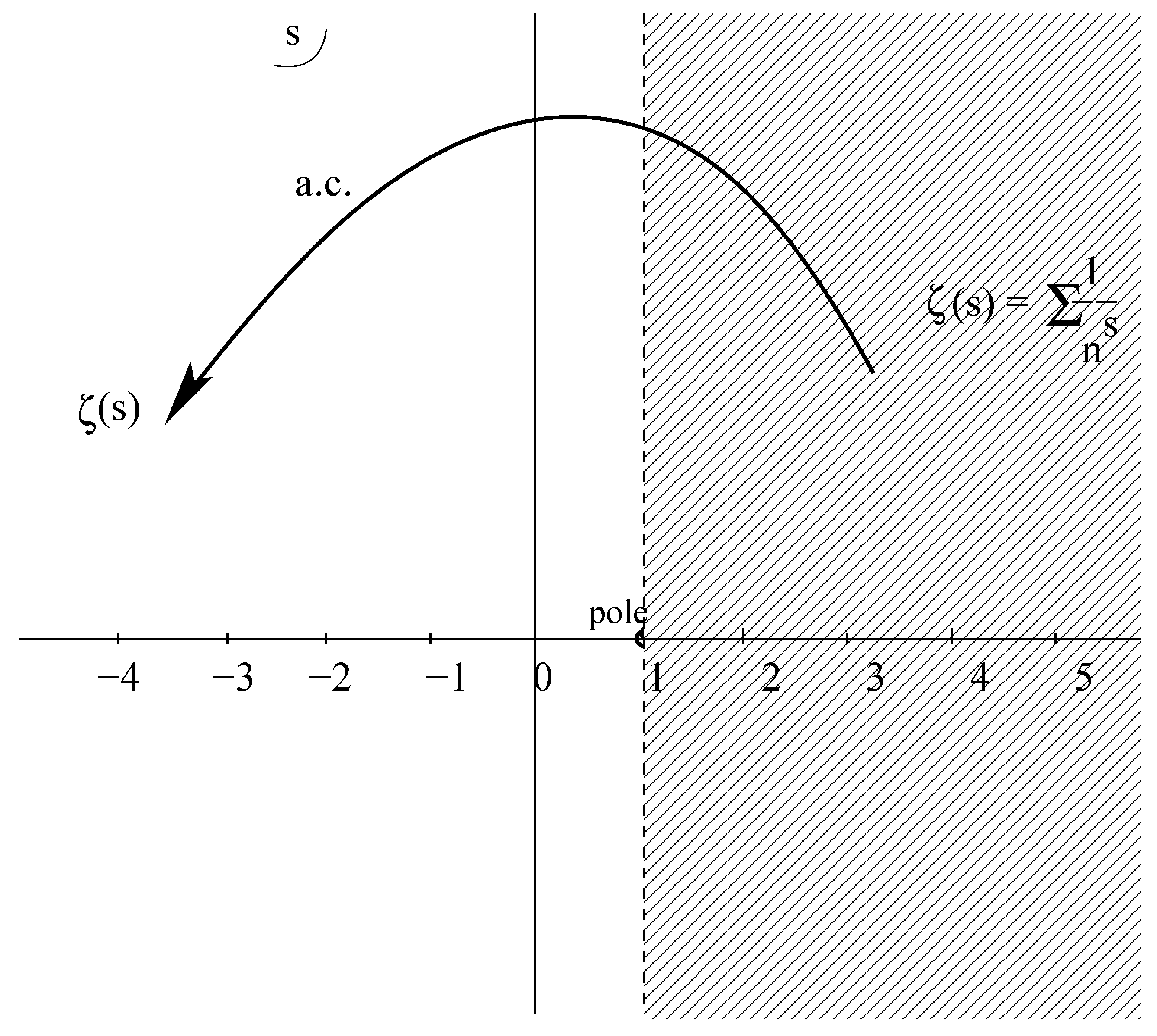
When we take now the Riemann zeta function, , with s complex, the series which defines it on the right half plane is absolutely convergent (for s on the right of the abscissa of convergence Re ). It remains, however divergent on the other half-plane. But it so happens that we can perform an analytic continuation of this function to that left part of the complex plane. In this way one obtains, finally, an analytic and finite function everywhere; with the only exception that it has a singularity, namely a simple pole, at (Figure 1). It is thus, a meromorphic function.5
In more general cases, the zeta function is associated with an operator—usually the Hamiltonian of the physical system. This case is in fact the most important for physical applications [34,35,55]. There, the process is essentially the same, although we should expect the derivation of the final formulas to be rather more difficult. Anyhow, under quite general conditions, a theory exists saying that for an ordinary Hamiltonian operator the corresponding zeta function will be also meromorphic, and that it will have a discrete sequence of simple poles, extending towards the negative side of the real axis of the plane.6
3.2. The Zeta Function as a Summation Method
From the construction of the zeta function carried out above, it is not difficult to guess how the summation method associated with it will proceed. We go back to the most simple example of all, the one at the very beginning, and then continue with similar cases.
- In view of the zeta function definition, we envisage the seriesas a particular value of the Riemann zeta, namely when . But this point is on the left half of the complex plane, as divided in two by the abscissa of convergence (Figure 1). There, the series as such diverges; but it is not the series, which gives the value of the zeta function there, not on that side of the plane. There, we must use its analytic continuation, which is nicely defined and yields a perfectly finite number, namely . ThusThis is therefore the sum of the series , when we view it as a particular value of the zeta function.
- Next, let us considerWithout more ado, we immediately recognize that this is the zeta function when the exponent is set to . We look at the value of the Riemann zeta there, and it turns out to be . Therefore,
At this point I cannot refrain from telling the reader some curious story, directly related with the above use of the zeta function; an experience I had some years ago, and not just once, but twice! Within an interval of less than two years, two highly distinguished physicists, Andrei Slavnov and Francisco Yndurain, came to give a seminar in Barcelona. It was not at the same time, and the subjects of their talks were quite different. But, what was extraordinarily remarkable was the fact that, on both occasions, the corresponding speaker turned towards the audience, at some point, staring for a moment at everybody’s face and said, with an authoritative voice, the same sentence, almost word by word: “As everybody knows, ”. In my understanding, the meaning was something like: The ones who do not know this, they better leave the room. It brought to my mind the statement written at the door of the Pythagorean school: Do not cross this door the ones who do not know Geometry.
An intriguing question that immediately appears on viewing these results is, how a series with all positive terms can eventually yield a negative result. This seems very strange and one could easily conclude that those mathematical manipulations, these analytic continuations on the complex plane can have nothing to do with real physics. In other words, this is a very extreme case of the unreasonable effectiveness of mathematics in the physical world. And it is in fact so, because using these weird results, as Slavnov and Yndurain and a lot many other practitioners do in QFT—to match the results of the most precise experiments in high energy physics ever done—show a coincidence with the experimental results of more than 15 digits. This is very spectacular [56,57]. The experiments carried out on the Casimir effect [2] show also a very good agreement, taking into account the problems one has to face to design and carry out such experiments in a properly controlled way [58,59,60].
Now, a not less important, computational issue. As we have seen, the zeta function regularization method relies on the analytic continuation of the corresponding zeta function. And the question is, how easy is it, in practice, to perform those continuations? Will this involve lengthy calculations every time, and on varying circuits of the complex plane? In fact this is not the case. From a theoretical viewpoint, the answer would be immediate: just use the reflection formula (or functional equation) of the corresponding zeta function. For the Riemann zeta (e.g., Equation (3)). In practice, however, such expressions are usually not very useful, for fast and accurate calculations; in fact, by using them we are going back to the series expansions we had at the beginning (the Riemann series again). This is however not the end of the story, since presently very effective new formulas have been found, converging exponentially fast on the whole complex plane (with the only exception of some singular points, since the zeta functions are meromorphic, generically), as the Chowla-Selberg [38] series formula and some others [39,42]. These identities endow with enormous power the method of zeta function regularization.
4. The Friedmann-Lemaître-Robertson-Walker (FLRW) Model and the Cosmological Constant
4.1. Towards the Observational Justification of the FLRW Model
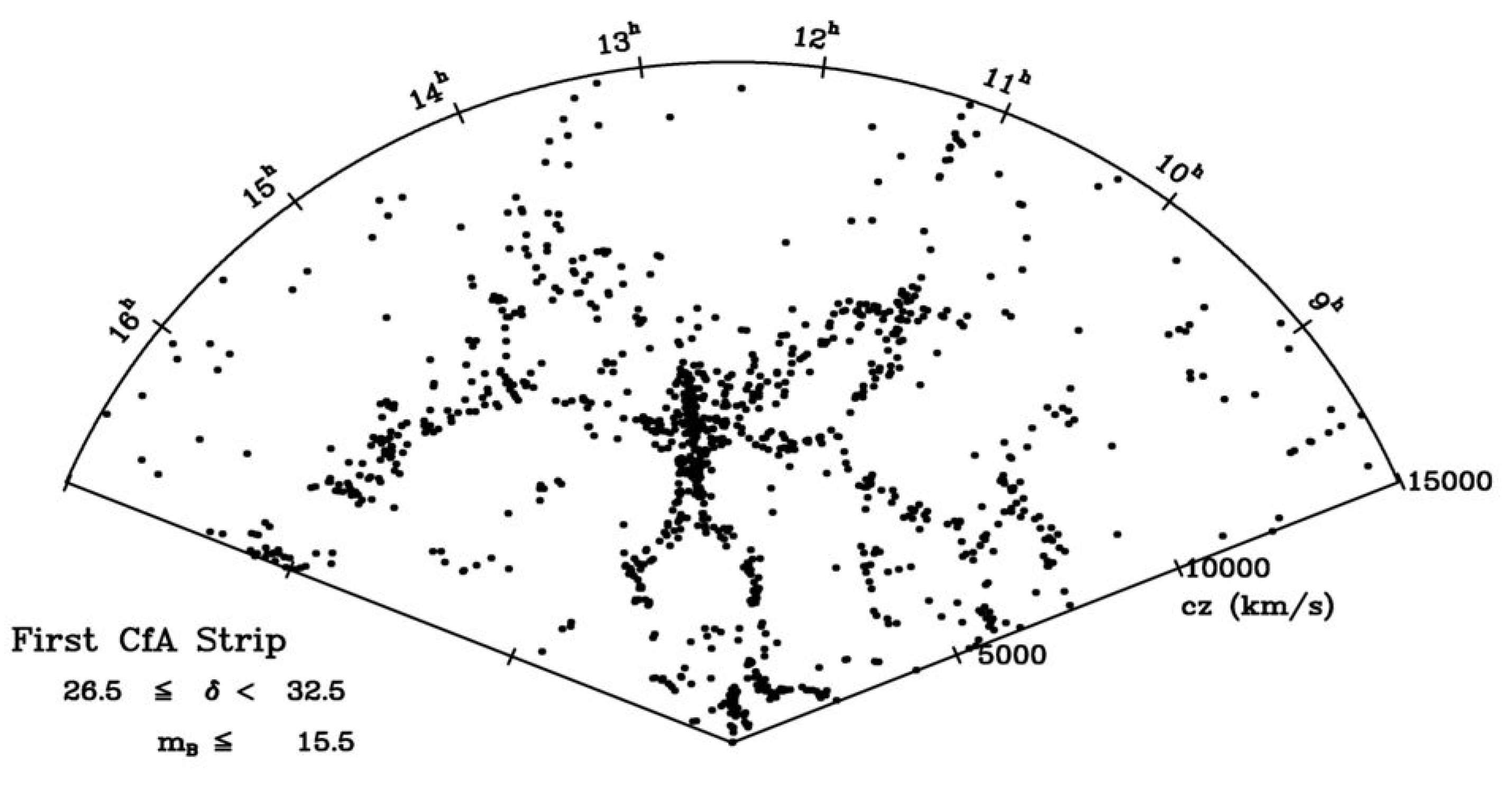
On a very large scale, that is, on a cosmic scale, celestial objects are points roaming in space. A glance at the first in-depth map of the Universe (Figure 2) is enough to realize this fact. Depending on their distance from Earth, the points will be galaxies with hundreds of millions (or billions) of stars, or galactic clusters with perhaps one million galaxies. On a cosmic scale, the Universe is a collection of points and, like any physical system, it is well specified if we know, along with their masses, their positions and speeds, so that we can represent them on the phase space. Unlike a laboratory system, in the case of the universe we always observe it from the same place, so the position of celestial objects will always be given, naturally, by the (radial) distance to the object and the two angular coordinates of the same, or equivalently, of its projection on the celestial sphere. Likewise, the velocity vector of each object will have a radial component, zooming out or approaching us, and another component perpendicular to the radial direction, which determines its displacement on the celestial sphere.
Now, in order to obtain a reasonable map of the large scale structure of the cosmos one needs precise values for the radial distance and, to get those, we need to calculate the redshifts of galaxies. Moreover, from those redshifts, their peculiar motions can be disentangled, too. These surveys do not have the issues of the projection effects of the maps in two dimensions. Notice that the last, which are just projections on the celestial sphere of the objects, were the only maps available up to merely thirty-five years ago. To be stressed again is the fact that not all the contribution to the redshift of a celestial object is due to the universal expansion (this is along the third dimension, the radial one); the peculiar velocities of the galaxies and clusters introduce additional contributions, due to their combined mutual attractions in the cosmic web. We can thus write, in first approximation:
This expression is obviously not exact, because generically the space is curved. If one does not take properly into account all the effects at play here, then one is bound to commit a number of errors in the maps. The so called “finger of God” effect, a long finger form pointing towards the observer, and other artifacts appear. Correction of all these effects is compulsory—and not so easy to do, in fact—to eventually get rid of such structures and obtain reliable three-dimensional maps of the universe.
A landmark in observational cosmology was set by the redshift survey due to de Lapparent, Geller and Huchra (the CfA survey of 1986 and 1988) [61,62]. Even if it was only “A slice of the Universe”, and even if it was a map at so large scale that just consisted of a distribution of black dots (each one corresponding to a whole galaxy), in this slice one could see, for the first time, the large-scale structure of our cosmos—a map of the universe in front of us for the very first time ever (Figure 2).
This survey, and the corresponding Southern Sky Redshift Survey (da Costa et al., 1988), [63] clearly showed that the voids were surrounded by filaments and walls [64] on the scales where the galaxy-galaxy correlation function can be neglected, “bubble-like” structures showed up in the galaxy distribution. Those maps had an immediate and enormous impact on the community of scientists. I personally witnessed that. Many physicists, who were working in quite different things, changed suddenly the direction of their research and started to try to explain, frame and reconstruct the point distribution as it appeared in this slice, trying to get this particular point distribution starting from some fundamental theory. Let me repeat this: until that day, 3 March 1986, all maps of the universe, even the magnificent Automatic Plate Measuring facility (APM) Galaxy Survey (Figure 3) with about three million galaxies, were two-dimensional, projections on the celestial sphere, what we would just see if we had extremely powerful eyes.
For an example, J. Ostriker, C. Thomson, and E. Witten [65] wrote a paper where, starting from string theory, they tried to explain the voids and the general structure of the map. I was also enormously impressed by the maps, too. Together with my student Enrique Gaztañaga, we had just come to me in search of a subject for his Master Thesis, we decided to study a more technical, but in no way less important question; namely, to find the best method in order to make the comparison of any two point maps. In any case, this was also a common problem with all the fundamental approaches. When a point distribution or map was produced by starting from a physical theory (or a phenomenological approach), the last step was always to quantify how good the map obtained using this approach was, as compared with the CfA survey map. For some time, the best method to do that was just using ‘the naked eye’. In fact, the apparently simple but enormously difficult question common to all approaches was: how good is the map obtained from such and such particular theoretical model with respect to the cosmological one? Certainly, Statistical Analysis gives a rigorous answer to this question, but it is given in terms of the two, three,…, point correlation functions of both point distributions. The problem is that all these point correlation functions must be calculated and compared, for any value of n. If all them are equal, for any n, then the two maps are equivalent. It goes without saying that such is a very cumbersome procedure, since higher-order correlation functions are difficult to compute when the point distribution has thousands of objects. Our aim was, therefore, to find an alternative procedure, more direct and optimized routes, leading to the highest unbiased information possible from the lowest number of distribution moments. That was the project. We considered, for instance, an elaborated counts in cells method as one of our first procedures. Indeed, this was the subject (or at least the starting point) of what finally evolved into Enrique’s PhD Thesis. By the way, he has become, with the passage of time, a world specialist on large scale structure. We did quite nice work together on these matters, later extended by Pablo Fosalba and Jose Barriga with considerable success, too. And this was the seed that gave eventually form to the theoretical cosmology group at the Institute for Space Sciences (ICE) and Institute for Space Studies of Catalonia (IEEC), in Barcelona, of which I feel now enormously proud.
The first catalogue gave rise and was followed by two other redshift surveys, namely the Infrared Astronomical Satellite (IRAS) survey and the Queen Mary and Westfield College, Durham, Oxford and Toronto (QDOT) survey. Thus, the original, only few thousands of galaxies of the CfA survey soon turned into the several millions monitored by the 2 Degree Field survey, 2dF, the Sloan Digital Sky Survey (SDSS), and so forth. In Figure 4, we show the results of the 2dF survey. When we compare the two images we immediately appreciate the enormous progress in observational cosmology that was done in only fifteen years.
From those observations it could be already concluded that the large scale galaxy point distribution had a dominant sheet-like structure. Moreover, it was just the scale of the survey what limited the scale of the sheets. It was also determined that the “great wall” structure (Geller and Huchra, 1989) [66] had been enhanced by the sample’s selection function, although it appeared in other deep wide angle surveys, too. Whatever the case, this was not the end of the discussion on that issue. Closer analysis showed that great walls not always bound great voids, instead, they surround families of not-so-great voids, bounded on its turn by not-so-great walls. It was suggested that maybe the great walls were picked out and then correlated by our own eyes to mentally construct larger structures [67]. N-body models also suggests this kind of effect because it was shown to be easy for our brain to identify coherent structures on scales where there was physically impossible that structures could be generated [64]. This clearly showed that naked eye analysis were not reliable. The progress since then has been impressive (for more information, the reader is addressed to these key project pages [68,69,70,71,72,73]).
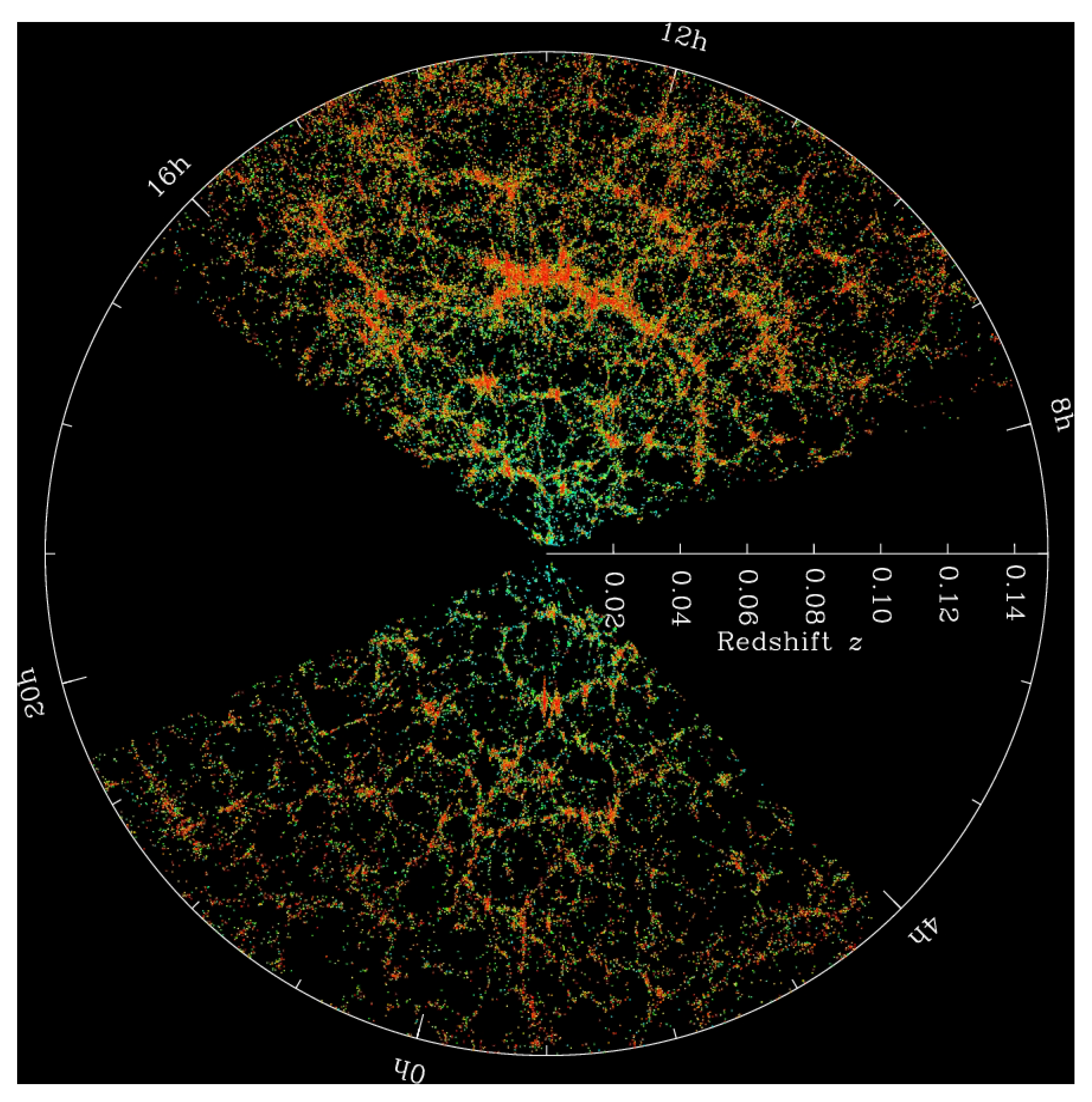
The now active operational phase of the SDSS project is SDSS-IV, https://www.sdss.org/collaboration/, which began on 1 July 2014 and is planned to run through 30 June 2020 at Apache Point Observatory, through early September, 2020 at Las Campanas Observatory, and to have a final data release in July 2021. The SDSS is carried out by an international collaboration of hundreds of scientists at dozens of institutions. SDSS-IV will be followed by SDSS-V, https://www.sdss.org/future/. The state of the art concerning this issue is given by the so called orangepie image of the universe up to redshift 0.15, the last galaxy map of the SDSS project, corresponding to data release 16 (Figure 5).
4.2. The Universe Is Indeed Homogeneous and Isotropic
The reader should we warned against confusing isotropy and homogeneity. Homogeneous is defined as “the same in all locations” while isotropic means “the same in all directions”. The pattern of a red brick wall, as the well-preserved ones we can still admire in Beacon Hill, in Boston, to put just an example, is homogeneous but it is not an isotropic pattern. The pattern of light rays emitted in any direction by a bulb or a candle in absolute darkness, on the contrary, is in fact isotropic, but it is not homogeneous. If we were placed in the middle of an infinitely large field, on top of a perfectly symmetric hill, while the rest of the field was completely flat, then, by looking around us we would see a perfectly isotropic landscape, the slopes of the hill being exactly equal in all directions. In this case, we would see isotropy, from our viewpoint, but the whole field would not be homogeneous, since there is this hill, we are sitting on top of.
Back again to correlation functions, it were accurate measurements of two-point correlation function for the galaxy distribution that provided the first direct evidence for the statistical homogeneity, at sufficiently large scales, in the cosmic matter distribution for the first time [74]. This long-standing problem was solved, in a first approach, by Totsuji and Kihara (1969) [75]. They concluded in their work that “The correlation function for the spatial distribution of galaxies in the universe is determined to be , being r the distance between galaxies. The characteristic length is 4.7 Mpc. This determination is based on the distribution of galaxies brighter than the apparent magnitude 19 counted by Shane and Wirtanen (1967). The reason why the correlation function has the form of the inverse power of r is that the universe is in a state of ‘neutral’ stability.” A good way to circumvent elaborated mathematical formulations in this matter is to get a deeper physical insight into the gravitational many-body problem. This is what Totsuji and Kihara did and allowed them to reach their conclusions. Previously, there had been intensive discussions on the different guesses at an exponential or Gaussian form for the correlation function. The mentioned results allowed to consider galaxy clustering as just a phase transition from an initial Poisson distribution to a final correlated distribution, which was slowly developing on always larger scales with the evolution of the universe.
The importance of these concepts comes from the fact that the cosmological principle is a very essential ingredient in modern cosmology. That is, the hypothesis that the universe is both homogeneous and isotropic, on large scales. It is the basis of the FLRW solution. This assumption has been confirmed and justified by studies of very different kind, in particular, of the distribution of large-scale structures in the universe and from very accurate analysis of the microwave background radiation. The announcement of the discovery of the Cosmic Microwave Background by Penzias and Wilson in 1965 provided already a quite strong proof of the homogeneity and isotropy of the cosmos. The deviations from homogeneity in the CMB radiation, as we now know, are in fact of about a part in ; what for a while made it even too homogeneous and created a severe problem when one wanted to find the necessary inhomogeneities, which should serve as seeds for star and galaxy formation. This problem has been solved in the meanwhile, with the new results that were obtained by the Wilkinson Microwave Anisotropy Probe (WMAP) and Planck missions. Very accurate maps of the whole universe showing the temperature fluctuations of the CMB have been produced, with increasing definition, by the Cosmic Background Explorer(COBE), WMAP and Planck. We show in Figure 6 the most recent Planck map.
It is not that easy to draw such maps. Many different effects and contributions, as dipole and quadrupole contributions, foregrounds, the galaxy plane contribution, observational biases, and many other, must be taken into account and conveniently subtracted from the raw image.
Provided big enough regions are considered, of some 100 Mpc or larger, our universe is seen to approach homogeneity, as measured now from the matter distribution. Concerning its isotropy, an updated approach can be found in Ref. [76].
4.3. On the Topology and Curvature of Space
The FLRW model for the universe corresponds to the only family of solutions of the Einstein’s field equations which has been shown to be compatible with the assumptions of homogeneity and isotropy of space. This is nowadays the standard model of the cosmos. But, we should remark that the FLRW one is in fact a family of solutions, with a free parameter, the curvature k, which can be either positive, negative or zero (the flat or Euclidean case). This curvature, or equivalently the curvature radius, R, is not fixed by the theory and should be determined from the cosmological observations. An important point is that the FLRW model, as is also the case with Einstein’s equations themselves, can only provide local properties, not global ones. These equations cannot give an answer to the question about the overall topology of the cosmos, on whether it is open or closed, or if it is finite or infinite. It is of course quite clear that, if not infinite, our universe is, in any case, extremely large, and very possibly we humans will never be able to reach more than just a tiny part of it. Even then, the posed question remains still very appealing. Note that all this discussion concerns only three dimensional space curvature and topology, time will not be here involved.
4.3.1. On the Curvature of the Universe
Probably, the first serious attempts to measure the possible curvature of the physical space go back to Gauss. With vertexes placed on the peaks of three German mountains, Brocken, Inselberg, and Hohenhagen, he tried to measure the sum of the three angles of the triangle that was formed. He was in search for evidence that the geometry of space was non-Euclidean. But one needs a much bigger triangle in order to find the possible non-zero curvature of space and the idea, although extremely brilliant for the time, was condemned to failure. More recently, cosmologist have measured the curvature radius R by using the largest triangle available at present, which is namely one with us at one vertex and with the other two situated on the hot opaque surface of the ionized hydrogen that delimits our visible universe and emits the CMB radiation, from some 370 to 380 thousand years after the Big Bang [77]. As is known, the CMB maps exhibit hot and cold spots (see Figure 6). It can be shown that the characteristic spot angular size corresponds to the first peak of the temperature power spectrum, which is reached for an angular size of (approximately the size subtended by the Moon) if space is taken to be flat. Spots should be larger (with a corresponding displacement of the position of the peak), if space has in fact a positive curvature, and correspondingly smaller if its curvature is negative.
Some years ago, the big amount of data obtained by balloon experiments (BOOMERanG, MAXIMA, DASI), combined also with galaxy clustering data, and submitted all together to a joint analysis, produced as a first result a lower bound for Gpc, that is, twice as large as the radius of the observable universe, of about Gpc.
More recently, the universe curvature has been measured using a combination of different techniques, by Planck (2018 data), also by using cosmic microwave background lensing, and baryon acoustic oscillation data. The Planck satellite, a joint effort between NASA and the ESA, did the latest effort to map the CMB across the whole sky. Planck measured the CMB to the greatest level of precision yet attained. Its most recent data were released in 2018 and from the CMB, as recorded by Planck, it seems that our universe might be closed, although the measurement is not significant enough. This is intriguing because, as we saw above, previous measurements suggested that our universe should be flat. In Ref. [78] it is claimed that without CMB lensing or BAO, Planck 2018 results show a moderate preference for a closed universe, with Bayesian betting odds of over 50:1 against a flat universe, and over 2000:1 against an open universe.
On the other hand, recent measurements of the cosmic microwave background by the Atacama Cosmology Telescope have found that the universe is flat, and with its density matching the critical density [79]: “We find no evidence of deviation from flatness supporting the interpretation that the [deviation seen by Planck] is a statistical fluctuation”. This was in answer to the tension coming from the Planck 2018 data analysis showing a deviation from flatness and a preference for a closed universe. This issue has not been closed yet, and it will be interesting to keep track of further developments on this point.
4.3.2. On the Topology of the Universe
As we said before, the equations for General Relativity do not determine the topology of the cosmos. Neither give they clues about the universe being finite or not. In the simplest case, our universe could perfectly be flat and finite. As of yet, there is no clear evidence against this. Anyhow, talking of other possibilities, of non-trivial topologies, from the theoretical viewpoint the most simple one is the toroidal topology (that of a tire, but three dimensional). The author of the present paper has profusely considered this topology before, in different aspects of the Casimir effect and, in particular, in relation with a possible Casimir effect at cosmological scale. We will return to this point later in the paper. And, indeed, there have been projects aimed at looking for traces of these and more elaborated topologies in the cosmos—as those corresponding to negatively curved but compact spaces—without success, in spite of the fact that some circles in the cosmic sky with near identical temperature patterns could be identified some years ago [80]. And still, from time to time, some paper appears proposing a new topology [81,82]. Anyway, summarizing all those efforts and the observational evidence, as of now: once biases on the numerical data are taken care of (what did not happen in some case, leading for a time to erroneous conclusions), we presently conclude that the available data point towards a very large (possibly infinite) flat universe.
4.4. The Cosmological Constant and Quantum Vacuum Energy
In GR the most easy and natural way to explain the accelerated expansion of the cosmos is to involve the cosmological constant. In this way, Einstein’s ‘great blunder’ might turn out to be in the end, quite possibly, one of his greatest discoveries. It seems to be the only way to explain the universal acceleration, within his theory, which has now become the standard theory of gravity, GR. There are, of course, some alternatives, extended gravities of different kind, but the standard cosmological model has been fixed to be, since some decades already, and remains so up to now, the CDM model. And this is so, in spite of the fact that the small value of the fitting has proven to be extremely difficult to explain.
In any case, for elementary particle physicists, the cosmological constant still constitutes now (in the words of J. Bjørken, pronounced long ago) “a great embarrassment’ [83]. But interpreted as a quantum vacuum contribution, the numbers are still off (if we compare them with physical data) by too many orders of magnitude. This has been an issue for a very long time, almost a century, if we consider that the problem started with the early discovery of the zero-point energy contribution in quantum physics.
In the 1980s, theoreticians tried to prove that should be zero (Coleman, Weinberg, Polchinski,…) [84,85,86,87,88,89,90]. This was already quite hard and no one succeeded. But we have now learned that should actually not vanish, although its value is very small. It might be indeed a true universal constant, as was namely the first thought of Einstein himself when he introduced it for the first time in 1917.
The cosmological constant is thus very important in cosmology, as we have just said [91] but, in complete independence (in principle) of the cosmic acceleration, it is also very important in the formulation of the local structure of fields and particles, as it shows up in the stress-energy density, , corresponding to the vacuum
Thus, the two contributions go together in the stress-energy tensor on the rhs of Einstein’s field equations: a possible universal constant and the contribution of the fluctuations of the quantum vacuum (allowed by Heisenberg’s uncertainty principle). Namely,
4.5. From General Relativity to Cosmology: On the Meaning of Einstein’s Equations
Consider the Einstein field equations including the cosmological constant term
where
Starting from the Einstein-Hilbert action,
these equations follow from a variational principle. They have a very deep and revolutionary physical meaning, as we all know [91,92].
Let us here recall the main principles that Einstein put inside, when he constructed his equations:
- In partial fulfillment of Mach’s principle, he established in his theory that the following ingredients were on the same footing: the space-time geometry (curvature), radiation energy, matter, and the cc.
- The geometric term, , would consist of a linear combination of the metric, , and of its first and second order derivatives, only.
- The energy-momentum tensor, would contain all possible forms of matter and energies in the universe, other than the gravitational one.
There is a very interesting discussion by Frank Wilczek on the fact that Einstein did not actually succeed in embedding in GR the whole content of Mach’s principle (see Ref. [93]). But actually many aspects of his theory, among them frame warping and frame dragging—by distributions of matter and rotating massive shells, respectively—can indeed be found in Einstein’s field equations.
In cosmology, an equivalent but much more employed expression for Einstein’s equation is the following one, which is given in terms of the redshift z (this can be viewed, in practice, as the inverse of the cosmological time):
If we look at it carefully, we will easily discover that this equation contains the whole (thermal) history of our universe. To this end, just notice that the different contributions are simply monomials in , of orders 4, 3, 2, and 0, respectively. For very small times, equivalently, when z is very large, the radiation term, of order 4, dominates over the rest. As time increases, z goes down, and for a specific value of z (which can be obtained equaling the terms of orders 4 an 3), a transition occurs from the radiation dominated epoch to that of matter domination. And so on, with the rest of the monomials. Subsequently, a curvature dominated epoch follows, until the cosmological constant term takes eventually over. The values for which these transitions occur are usually termed and , respectively, and they are given by
To summarize, the history of the universe, according to Einstein’s GR theory, goes through the following different epochs: it starts with radiation domination, then comes matter domination, then the curvature domination period, and finally the present epoch in which the cosmological constant dominates. That is, in very few words, the entire thermal history of our Universe. For more details, the reader is addressed to the following useful references [94,95,96,97].
5. Zeta-Function Regularization in Curved Spacetime
One can quite safely say that zeta-function regularization in physics was introduced by Stephen Hawking. Although, previously, there had been several published papers that had already used the basic idea behind it, it was Hawking who clearly defined the complete procedure for the first time [98,99], as a fundamental tool for carrying out the regularization of the infinities that appear in QFT in curved spacetime [100,101,102]. The main ideas behind the method, that justify departing from the more canonical procedure, are as follows [98,99]. In principle, Quantum Gravity can be approached by employing a canonical procedure, namely through the definition of a time arrow and by working then with equal-time commutation relations, on the space-like hypersurfaces perpendicular to it. But there are some arguments against this way of proceeding, among them the following ones:
- Many of the topologies for the space-time manifold are actually not product topologies, of the form , to allow such procedure.
- Some of these non-product topologies are actually quite interesting and worth of study exactly as they are, without unjustified simplifications.
- In view of the Heisenberg uncertainty principle, in quantum mechanical setups the meaning of ‘equal time’ looses precise sense and one is bound to look for alternatives.
It is then understandable that one turns to consider other procedures, in particular and most naturally, towards the path-integral approach
Here denotes the spacetime metric, the matter fields, are general spacetime surfaces (), is a measure over all possible ‘paths’ leading from the to the values of the intervening magnitudes, and S is the action, namely
R being the curvature, the cosmological constant, g the determinant of the metric, and the Lagrangian of the matter fields. Then, by imposing that the action S be stationary under the boundary conditions
one obtains the Einstein field equations:
Here, is the energy-momentum tensor of the matter fields,
In curved spacetime backgrounds, the path-integral formalism provides a way to deal with QFT ‘perturbatively’ [101]. One first, defines an Euclidean action by means of a rotation in the complex plane, as
and by substituting , one can then introduce, in a most simple way, the finite temperature formalism, which yields the partition function:
And now if, as is usual, the Feynman propagator is obtained as the limit of the thermal propagator for , then it comes into play the very interesting result we obtained some time ago [103], namely the usual principal-part prescription in the zeta-function regularization method (to be described below) need not be imposed as an additional assumption, since it beautifully follows from, and thus can actually be replaced by, this more general (and natural) principle [103]. Ours was quite a remarkable result for completing the formalism.
In order to calculate the path integral, usually the stationary phase approach is used. It is also known as the one-loop, or WKB approximation and proceeds by performing an expansion around a fixed background, as follows
what leads to the following result in the Euclidean metric:
The result is very conveniently expressed in terms of determinants, corresponding to the bosonic and/or fermionic fields which appear in the calculation. If we denote with A and B the respective pseudodifferential operators associated with the physical quantities in the Lagrangian, we have
As advanced, the result is given in terms of determinants for the bosonic and fermionic fields, respectively. And that would be the end of this very brief introduction to the method. We will now see how these determinants can be regularized by using the zeta function procedure.
5.1. Some Words on the Calculation of the Determinants
Now comes the next step. It is well known, and we have just provided an example of this fact, that in QFT many calculations reduce, essentially, to compute the determinants of the differential operators associated to the relevant physical quantities. At one-loop order at least, we could briefly conclude that all QFT theories reduce to theories of determinants. Most physicists would say, wrongly, that the operators involved in the calculations are ‘differential’ ones. However, if we want to speak properly, this is not so, given that in many of the cases they are actually pseudodifferential operators (DO). We will not enter here into the precise definitions, which can be found in the literature and, moreover, I have given them elsewhere in very comprehensible terms [35,42]. Loosely speaking, we could summarize that those are ‘analytic functions of differential operators’, such as (here D is a differential operator) or . However, one should be careful with some functions, for example, , which are not valid in this sense, since they do not yield a DO. The theory of DOs is explained in References [42,104,105,106,107,108,109,110] in much detail.
We have just discussed the importance of the concept of determinant of a differential or DO in theoretical physics. It is, therefore, very surprising that their study is not more extended among mathematical physicist or function analysts. I should qualify my statement, by adding that what I mean is the calculus of the determinants discussed above, which appear in QFTs and always require a regularization process in order to be defined properly, since they are divergent. The corresponding mathematical operators are not of the trace-class, which is the theory well studied by mathematicians. These calculations involving divergent determinants have a lot in common with the calculation of divergent series that we have considered above—the series usually appear as (divergent) traces of infinite determinants. However, in the case of determinants there is no general reference comparable to Hardy’s book [6] mentioned above. Without pretending to have filled that gap completely, this may somehow explain the remarkable success of my books on this subject (see below).
Actually, from a general viewpoint one could argue that the question of regularizing infinite determinants had been already addressed, and solved in some way, by Weierstrass. Although his approach has been successfully employed by some theoretical physicists with success, as a general procedure it is not so valid, since it has serious problems. In fact, non-local contributions appear, generically, and they lead to results that cannot be given a physical meaning in ordinary QFT. For completion, it should be mentioned that, since long ago, for more usual differential operators there are, of course, well-defined theories of determinants, as for instance, for degenerate operators, for trace-class operators in the Hilbert space, for Fredholm operators, and so forth [111]. These theories are also of much use in physics, but it turns out that these definitions of determinant do not solve any of the problems above, which arise in QFT and can only be cured by resorting to a regularization procedure.
5.2. An Update of the Most Influential Contributions on Zeta Function Regularization
An update of the pioneering and most cited contributions on the subjects above, and on its considerable impact in different research fields, follows. When searching the Google scholar webpage, on 15 November 2020, for the best cited works on the very general subject of “zeta regularization”, we encountered only two works surpassing the one-thousand citation milestone. The first in number of cites is no other than Hawking’s seminal paper of 1977 on zeta function regularization, already mentioned before [98]. In this work, the method was very clearly defined, as summarized above, for the first time and in a highly pedagogical way. The aims and usefulness of the procedure were very well explained, in dealing with quantum field theories on curved spaces. The second top cited reference, with more than one thousand citations, too, is a book written by the author of the present paper, together with four collaborators, in 1994 [34].
The third most cited reference is the also seminal article by Dowker and Critchley on the practical uses of the zeta regularization method [112], written in 1976, prior to the work by Hawking, and which has got almost 900 citations. And the forth most cited reference on the subject, approaching the 700 citation mark, is another book of 1995 published by Springer Verlag, and written by the author of the present paper alone [35]. This book has been considerably improved and enlarged in a second edition issued in 2012. Those are by far the most influential works—attending to the number of citations they have accumulated up to now—written on the subject of zeta function regularization and its applications in physics.
To complete the search, in the immediately following range, which comprises works with four and three hundred citations plus, we found the following: a book by K. Kirsten [113] and two papers, one by S. Blau, M. Wisser and A. Wipf [114], and a paper by M. Bordag, the present author and K. Kirsten [115]. Although this should be pretty obvious, I find it necessary to remark that to get these amounts of citations in such a technical and highly mathematical subject as zeta regularization is not so easy.
Our already mentioned book [34], followed by a review by D. Vassilevich [116] with some 870 citations and our paper above [115] lead the list of most cited references on the subject of “determination of heat kernel coefficients”, when searching again in Google Scholar. Indeed, using the techniques of zeta function regularization we were able to find what is still, as of now, an unchallenged method for the exact derivation of the heat kernel coefficients to any order, provided the series expansion of the symbol of the corresponding pseudodiferential operator to this same order is available. This was also a revolution in the field and gave rise to a large number of subsequent papers and review reports. It is an extremely fruitful practical use of the method of zeta function regularization for operators which spectrum is not known explicitly, a very interesting subject by itself.
6. Quantum Fluctuations of the Cosmological Vacuum Energy
6.1. Two Examples of the Use of the Zeta Function Method
The discovery of the accelerated expansion of the universe by two different groups some twenty years ago [117,118,119,120,121] brought back to the forefront the discussion of the possible existence of a non-vanishing cosmological constant. In fact, after many profound studies, data analysis corresponding to accurate astronomical observations, and after lots of new data have been gathered—what is very important, from absolutely independent perspectives—and after hot discussions on possible alternatives or generalizations of the Einstenian GR theory, the present accepted model of the universe, adopted as the standard cosmological model, is the so called CDM model, or cold dark matter model with a small cosmological constant [96,122,123].
Following these first pioneering works in which the cosmic acceleration was discovered, some balloons were flown that confirmed the first results, in particular BOOMERAanG [124] and MAXIMA-1 [125,126]. Later, confirmatory evidence has been found in the analysis of baryon acoustic oscillations (BAO), in analyses of the clustering of galaxies at large scales [127,128,129,130,131], in much more extensive and precise supernova observation [132], in precise determinations of the age of the universe, and in the results coming from gravitational waves as standard sirens. Finally, the most simple solution, and which is in accordance with the astronomical results, has been to recover Einstein’s cosmological constant term. Its precise value has been fixed, in the available models, from the data coming from those observations [133,134,135].
It was Weinberg who said some time ago in a review paper [136] that it was “even more difficult to explain why the cosmological constant is so small but non-zero, than to build theoretical models where it exactly vanishes”, what was already hard enough [84,85,86,87,88,89,90]. The original discrepancy between the observed value of the quantum fluctuations of the vacuum state of the fields pervading the universe, which should be observed in fact, and the value coming from the universe acceleration, which according to crude order of magnitude estimations in terms of a cut-off of the Planck order (beyond which QFT is no more reliable), was of some 123 orders of magnitude. It has been reduced somehow, according to several theories of very different kind. However, the discrepancy continues to be still very large.
The fine-tuning cancellation of such enormous values is very difficult to grasp and a very hard question to answer. Rather than following this way, in this section we will review a simple model, coming from an idea that was proposed by the author some time ago. The idea is to consider different possible topologies of the universe, with some of its three large dimensions compactified, and with a number of extra dimensions, of the order of the Planck length, some of which might be compactified, too. One thus deals with the global and local topology of the universe [137]. A second ingredient was a possible scalar field pervading the universe. In inflationary models, quintessence theories, and modified gravity theories of several kinds this sort of fields are common. We did not address the old problem of the cosmological constant, which is extremely hard to solve. We just constructed a simple toy model to shows that one could easily obtain some contributions to of the right order of magnitude, that is, the one dictated by the astronomical observations [117,118], that is, erg/cm. It was namely the new cosmological constant problem, according to Weinberg’s terminology [136], which we addressed there.
To summarize, one starts by assuming that the bulk value of the cosmological constant (the one corresponding to the flat case) is zero, by invoking a mechanism of a fundamental theory (as of now not fixed), which will do this job. In other words, we are confident that the old problem of the cosmological constant will be solved, sometime. Then we assume the existence of a scalar cosmic field background, of very small mass, and the contribution to the cosmological constant is calculated as coming from the Casimir energy density [2] corresponding to this field, for some specified boundary conditions, and as a consequence of those being imposed. On top of the three large spatial dimensions (some of which may be compactified) one also assumes there might be one or two small extra dimensions; again they can be compactified or not.
As we have mentioned, there is an extensive literature in the subject of what is the global topology of spatial sections of the universe [137] and also on the issue of the possible contribution of the Casimir effect as a source of some sort of cosmic energy, as in the case of the creation of a neutron star [138]. Also, there are arguments that favor different topologies, as a compact hyperbolic manifold for the spatial section, what would have clear observational consequences [139,140,141]. Interesting work along these lines was reported in Ref. [32,33] and related ideas were discussed in Ref. [142]. However, our approach was different from all these. Our emphasis was put in just obtaining the right order of magnitude for the effect. The different possibilities concerning the nature of the field, the different models for the topology of the universe, and the various possible boundary conditions, with corresponding effect on the sign of the force, were not investigated.
The models considered in the paper, for the space-time topology, were of the two types: , . The equation satisfied by the free scalar field of (very small) masss M is
where D is here the d’Alembertian operator. On top of it, one now imposes the corresponding boundary conditions (periodic, in the first considered case, antiperiodic, for fermion fields, or possibly of mixed sort). is here the number of non-compact dimensions.
If H is the Hamiltonian of the massive scalar field and the vacuum state, the expression for the zero-point energy, is . This is to be subtracted from the corresponding expression where the boundary conditions associated with the compact dimensions (large and small) have been imposed. Actually, this is very conveniently performed in practice by just sending the compactification radii (after making them dimensionless, by way of introducing a regularization constant, ) to infinity. As usual in Casimir calculations, these two vacuum energies will individually give an infinite result; however, their difference yields a finite final result
Here R is a typical compactification length. The Casimir energy will depend on , after the regularization process is carried out. In fact, this is the Casimir (or vacuum) energy density, , which can account for either a finite or an infinite volume (in a corresponding limit) of the spatial section of the universe. Subsequent renormalization will render the final result independent of the regularization parameter, .
Let me here say a few more words on this method and the expressions above. As compared with the more standard definition and use of the Casimir energy associated with the introduction of two plates (or corresponding boundary conditions) on the vacuum state of a quantum physical system—and then subtracting the case where there are no plates (or BCs) from the case where they are in place—the situation in cosmology is a little bit different. Frequently, I have been asked in my oral presentations of the subject the following questions: Where are here the plates? How can you talk of Casimir energy or Casimir effect in such situation? One should notice that the essential point in the Casimir calculation is not the presence or absence of the two plates, but the comparison between two close cases, both corresponding to the calculation of the vacuum energy density of the same quantum system but in two different situations. And those are not just restricted to the presence vs absence of a pair of plates, but they include, for example, the presence or absence of a background field, or of some spatial curvature, or of some sophisticated kind of boundary conditions, and so forth. In the set up at hand, we are comparing the case of a universe with some spatial curvature with the flat case, where the curvature is vanishing [143,144,145,146,147,148].
The idea presented in our work was not entirely new. However, the simplicity and the generality of its implementation were absolutely original. The strategy proposed was completely independent of any concrete model, under the assumptions listed before. Moreover, the only free parameters to play with, namely the number of compact dimensions and the values of the compactification radii, were in fact very much constrained, at least in the case of the small additional dimensions, by the necessity to recover admissible values7, in accordance with other theories and observations. Also to be remarked is the fact that the calculation was not easy at all to carry out. Fortunately, some very powerful reflection identities, obtained in previous work by the author, could be used, which allowed to obtain an analytic result.
Summarizing the final results we got, a good coincidence with the observational value for the cosmological constant was obtained for the contribution of a close to massless scalar field, , for p large compactified dimensions and small compactified dimensions, , and this for values of the small, compactification length, b, of the order of 100 to 1000 times the Planck length , what are very reasonable values, in view of other theories. The best agreement was reached for cases where there was one small compact dimension in excess of the number of large compact ones.
To be also remarked is the fact that the treatment was not just restricted to toroidal compactifications, since spherical ones and mixed toroidal (for small dimensions) and spherical (for big ones) compactifications could be treated analogously. Both these cases correspond to observational isotropic spatial geometries. One should remark also that, already at this level, the calculations were rather involved; although the use of zeta function techniques, in particular of the generalized Chowla-Selberg series formula, could finally render analytic results. Contrary to some guesses, simple power counting proved to be unable to provide the correct order of magnitude of the outcome.
On dimensional grounds, all results were dictated by the two basic lengths of the problem: the Planck length and the value of the size of the observable Universe. Playing with these two scales and performing a precise calculation of the Casimir effect, it was shown that the observed value of could be remarkably well fitted, for the most commonly considered models of the space-time topology. And all them corresponded to a marginally closed universe, in full agreement, too, with other completely independent analysis of the observational data [96,117,118].
Many questions were posed, in the meanwhile, on these oversimplified models, e.g., concerning the dynamics of the scalar field, its couplings with gravity and other fields, a possible non-symmetrical behavior with respect to the large and small dimensions, or the relevance of vacuum polarization (see Ref. [149,150,151] concerning this last point). One can argue that they will probably not have much impact on the final result, but indeed, one should address these issues in a more elaborate model. Interesting to observe is that, in particular, the mass obtained for the scalar field in Ref. [152], was extremely close to our own result.
In addition, the existence and specific properties of the cosmic microwave radiation (CMB) mimics, in a way, the situation we described, since the ‘mass’ associated with the CMB radiation is also in the sub-lightest-neutrino range. The existence of scalar fields with a very low masses also appears in other theories, as in SUSY models, when the scaling behavior of the cosmological constant is considered [134].
Finally, one should again recall that, indeed, the presence of the quantum vacuum energy is ubiquitous, and that the Casimir effect appears (sometimes inadvertently) in many different situations. Its contribution is sometimes very small, as in the case of sonoluminiscence, in other occasions of some 10 to 30% of the complete effect, as is the case in wetting phenomena, involving He3, in condensed matter physics, and so on. In the case of cosmological applications, its importance has to be still appreciated and the results reviewed here could open a door to a new domain of activity. This may take time, as is happening with other projects, as is the case of the intended use of the Casimir force in outer space for small vehicle propulsion, and other uses.
6.2. A Brief Update on the Dynamical Casimir Effect
There is a very long and outstanding review of the dynamical Casimir effect, actually a a digest of the main achievements in this wide area for the past 50 years in Ref. [153]. Here, I will just summarize in a very succinct way some of the contributions of our group in this subject, mainly with a view to cosmological applications.
As very well explained in Ref. [153], it was in 1969 when G.T. Moore [154] in his well known PhD thesis (almost 700 citations up to now in Google Scholar) showed that motions of ideal boundaries of a one-dimensional cavity could generate electromagnetic field quanta from the vacuum. In 1975 B. DeWitt in his very famous book [155] (over 1600 citations as of now) demonstrated that moving boundaries could induce particle creation from the quantum vacuum in a single-mirror, and one year later S.A. Fulling and P.C.W. Davies [156] published an also very successful study (it has collected almost 800 citations to date). Not to forget is moreover the influential 1982 contribution by L.H. Ford and A. Vilenkin [157]; and, some years later, the two References [158,159]. This area has developed enormously, suffice to say that the mentioned review by Dodonov contains as many as 558 references, and it is for me impossible here to do justice even to a small percentage of them.
The contributions of our group to the dynamical Casimir effect in cosmological problems is generously mentioned in Ref. [153]. In a PRL paper with Jaume Haro [160], we developed a consistent approach to the dynamical Casimir effect; in Ref. [161] we constructed a physically sound Hamiltonian formulation of the same and, subsequently, we applied the dynamical Casimir effect with semi-transparent mirrors to cosmology [162]. Moreover, we also simulated black hole collapse by vacuum fluctuations using a moving semitransparent mirror [163]. As a summary of the main ideas of our development, we formulated a mathematically rigorous, an analytic, theory for the very physical situation of partially transmitting mirrors, which become transparent to very high frequencies. And, remarkably, we could express the whole process by means of an analytic matrix. We then proved both: (i) that the number of created particles was finite, and (ii) that their energy is always positive, for the whole trajectory during the displacement of the mirrors. And, also, that the radiation-reaction force acting on the mirrors owing to emission-absorption of particles is related with the energy of the field, through the energy conservation law. This provided a closure to the whole formalism, which ended in a Hamiltonian method for a neutral Klein-Gordon field in a cavity, with boundaries moving at a certain speed, as in Ref. [164].
We also made the important observation that in the seminal Davis-Fulling model, mentioned above [156], the renormalized energy is negative—while the mirror moves, the renormalized energy cannot be considered as the energy of the particles produced at time t (cf. paragraph after Equation (4.5) [156]). And our interpretation was, finally, that a perfectly reflecting mirror is actually non-physical. This is because, instead, any physical mirror will be a partially transmitting one: it will become transparent to high-enough frequencies. That our formulation of this imperfect, but physically realistic case could be done using an analytic matrix—a true physical situation in a nice and perfectly controlled mathematical setup—was a remarkable result, with potentially very important applications, what one can closely follow in the works already mentioned.
In a paper written some years back, by members and collaborators of our group [165], the dynamical Casimir effect was discussed in the context of quantum cosmology. The background field method and the effective action formalism were used to describe the four-dimensional dynamical Casimir effect. The picture was that of quantum cosmology for an expanding FLRW universe—the boundary conditions acting as a moving mirror—filled by a conformally invariant quantum massless Grand Unified Theory (GUT). The cases in which the static Casimir energy is either repulsive or attractive were considered. Inserting the simplest possible inertial term, in the adiabatic (and semiclassical) approximation, the dynamical evolution of the scale factor and the dynamical Casimir stress were obtained, analytically and numerically, depending on the complexity of the situation, for the SU(2) super Yang-Mills theory. Thus, a formalism was developed to describe the dynamical Casimir effect in the adiabatic approximation, which could be applied to arbitrary GUTs, extensible in principle to any specific four-dimensional background, although the discussion in the paper was limited to a toroidal FLRW universe, providing the moving boundary conditions. The main limitation of the approach was the mentioned compulsory restriction to the adiabatic approximation.
6.3. An Update of the Impact of Papers on Zeta Functions and Cosmology
When searching on the web, and in particular, in the convenient tool provided by Google Scholar, for the combination of words “cosmology” and “zeta”, the most prominent reference that does appear is, by far, the aforementioned book by the author Ten Physical Applications of Spectral Zeta Functions [35], with ca. 700 citations. It is followed by a paper by S. Christensen and M. Duff, where these authors introduced a generalized zeta function in order to quantize gravity with a cosmological constant term, which totals ca. 350 citations [166], a paper by the author alone, on the cosmo-topological Casimir effect, which appears when treating QFT with boundary conditions by means of the zeta-function method [167], with some 110 cites, a paper by I. Aref’eva and I. Volovich on the quantization of the Riemann zeta function and cosmology [168], with some 70 citations, and another paper of the author, cited over 60 times, on matching the observational value of the cosmological constant [169]. And by a number of other papers with more limited impact, when measured by the number of cites. We conclude that, in comparison with other searches, this combination is not so commonly referred to.
However, the situations changes radically when we search for references on the “cosmological constant”. During the last decades this has been from time to time an extremely hot problem, what is reflected by the very large number of citations of the top works on this issue. To wit, the close to 7000 cites of the renowned review by S. Weinberg “The cosmological constant problem” [84], the 5000 citations of the review by P.J.E. Peebles and B. Ratra “The cosmological constant and dark energy” [170], the 3250 citations of the report by T. Padmanabhan “Cosmological constant—the weight of the vacuum” [171], the 2750 citations of the PRL paper by I. Zlatev, L. Wang and P.J. Steinhardt “Quintessence, cosmic coincidence, and the cosmological constant” [172], and the 2300 cites of S. Carrol’s review “The cosmological constant” [96]. All these figures are, however, dwarfed by those of the two very famous papers announcing the discovery of the accelerated expansion of the cosmos, by A.G. Riess et al. [118] and by S. Perlmutter et al. [117], with over 20000 and 19000 citations, respectively. It is just impossible to compete with the extraordinary impact important astronomical publications have, nowadays.
From the theoretical side, there are, in addition, a good dozen of papers that have got over one thousand cites. Let us just select a few: those of S. Coleman [86,87] and of C. Wetterich [173], of the old wave, and a paper by A. Starobinsky [174] and our paper [175], which together with [176] they discuss alternative approaches to the issue in modified theories of gravity. Actually, there have been many different attempts to find a solution to this very hard problem. I just quote here, to finish, the most recent, brand new approaches, of the last couple of years, at solving the cc problem, by Unruh, Leonhardt, Carlip, Santos, and others [177,178,179,180,181].
7. Summary and Conclusions
In this paper we have given a very basic overview, of pedagogical nature, of the zeta function method, with emphasis on the basic concepts and on the historical background of the procedure. The main purpose has been to complement other works, in particular some of the author, which contain mathematically rigorous presentations, but where this basic but not less important perspective was missing. The method has then been used in the paper, for the regularization of physical quantities, such as quantum vacuum fluctuations in several contexts, always taking advantage of the insight one gets from very basic examples.
The first part of the paper has been devoted to the just mentioned historical context of the zeta function regularization method. Contrary to what happens with other procedures, in particular with cut-off techniques, these analytic continuation methods are considered, by many, to be highly unnatural and counter-intuitive, since one looses track of what is happening during the mathematical computation. This is why we started our discussion by putting the issue into the general framework of the unreasonable effectiveness of mathematics in physics an the other sciences. After a very short introduction on the Riemann zeta function, its uses as a summation method, and its generalization to the concept of zeta function of the relevant mathematical operator corresponding to the given physical quantity (commonly, the Hamiltonian of the quantum system under consideration), we have summarized the main steps of the method of zeta function regularization.
In the rest of the work, we discussed the regularization of quantum vacuum fluctuations in different setups and, specifically, we have employed the method to obtain reasonable, physically meaningful values for the relevant quantities considered. Notably, in the case of the Casimir effect at cosmological scale, as a possible and very natural contribution to the cosmological constant. A brief update on the dynamical Casimir effect, also in view to cosmological applications, closed that part of the work. In addition, recalling a couple of simple and explicit examples, with the aim to demonstrate how zeta function regularization works in practice, we have stressed the elegance and power of the procedure for dealing with rather non-trivial calculations in curved spaces with compact dimensions. Remarkably, this can be done in an analytic, exact way, by using our extension of the powerful Chowla-Selberg series formula.
Towards the end of the paper we have presented an updated retrospective view of the developments of these subjects and applications during the past years, with specific reference to the pioneering and most influential papers (according to their number of citations) in different aspects of those approaches, aims and directions.
We finish with a consideration of some possible future applications of the zeta function method in cosmology. There is at present considerable activity, and truly promising studies are being carried out on several subjects involving this connection. They have been initiated in recent years and could blossom and render good surprises in the not so far future. Among them, studies on: Zeta functions, anomalies and stable branes, on zeta functions in braneworld cosmology, on cosmological uses of the quantization of the zeta function, on applications of related elliptic and theta functions to the FLRW cosmology, on uses of the zeta function in Friedmann models with viscous cosmology, in modified gravity theories, in multiscale gravities, in the quantization of gravity in the presence of a cosmological constant, and many other issues, in addition, that the reader may easily find just by examining the available literature.
Funding
This work has been partially supported by MCI/AEI/FEDER, European Union, projects FIS2016-76363-P and PID2019-104397GB-I00, and by AGAUR (Catalan Government), project 2017-SGR-247.
Acknowledgments
The author is very much obliged with his numerous collaborators along many years of work on those subjects. They are too many to be listed here, but their names can be read from the papers coauthored, in the bibliography of the present work. Two anonymous referees provided also very useful comments that helped to improve the manuscript substantially.
Conflicts of Interest
The author declares no conflict of interest.
References
- Wigner, E. The unreasonable effectiveness of mathematics in the natural sciences, Richard courant lecture in mathematical sciences delivered at New York University, May 11, 1959. Commun. Pure Appl. Math. 1960, 13, 1–14. [Google Scholar] [CrossRef]
- Casimir, H.B.G. On the attraction between two perfectly conducting plates. Proc. K. Ned. Acad. Wet. 1948, 51, 793–795. [Google Scholar]
- Turnbull, H.W. The Great Mathematicians; New York University Press: New York, NY, USA, 1961. [Google Scholar]
- Alton, E.J. Encyclopedia of World Biography; McGraw-Hill: New York, NY, USA, 1973; Volume 4, pp. 30–31. [Google Scholar]
- Maor, E. To Infinity and Beyond: A Cultural History of the Infinite; Princeton University Press: Princeton, NJ, USA, 1991. [Google Scholar]
- Hardy, G.H. Divergent Series; Oxford University Press: Oxford, UK, 1949. [Google Scholar]
- Cao, T.Y.; Schweber, S.S. The conceptual foundations and the philosophical aspects of renormalization theory. Synthese 1993, 97, 33–108. [Google Scholar] [CrossRef]
- ’t Hooft, G.; Veltman, M. Regularization and renormalization of gauge fields. Nucl. Phys. B 1972, 44, 189–213. [Google Scholar] [CrossRef] [Green Version]
- Pauli, W.; Villars, F. On the Invariant Regularization in Relativistic Quantum Theory. Rev. Mod. Phys. 1949, 21, 434–444. [Google Scholar] [CrossRef] [Green Version]
- Creutz, M. Quarks, Gluons and Lattices; Cambridge University Press: Cambridge, UK, 1985. [Google Scholar]
- Politzer, H.D. Reliable Perturbative Results for Strong Interactions? Phys. Rev. Lett. 1973, 30, 1346–1349. [Google Scholar] [CrossRef] [Green Version]
- Gross, D.J.; Wilczek, F. Asymptotically Free Gauge Theories I. Phys. Rev. D 1973, 8, 3633–3652. [Google Scholar] [CrossRef] [Green Version]
- Wilson, K.G.; Kogut, J.B. The renormalization group and the ϵ expansion. Phys. Rep. 1974, 12, 75–199. [Google Scholar] [CrossRef]
- Zinn-Justin, J. Quantum Field Theory and Critical Phenomena; Oxford University Press: Oxford, UK, 2002. [Google Scholar]
- Scharf, G. Finite Quantum Electrodynamics: The Causal Approach; Springer: Berlin, Germany, 1995. [Google Scholar]
- Blanchet, L.; Faye, G. Hadamard regularization. J. Math. Phys. 2000, 41, 7675–7714. [Google Scholar] [CrossRef] [Green Version]
- Hadamard, J. Lectures on Cauchy’s Problem in Linear Partial Differential Equations; Dover Publications: New York, NY, USA, 1923. [Google Scholar]
- Atiyah, M.F.; Singer, I.M. The Index of Elliptic Operators on Compact Manifolds. Bull. Am. Math. Soc. 1963, 69, 422–433. [Google Scholar] [CrossRef] [Green Version]
- Atiyah, M.F.; Singer, I.M. The Index of Elliptic Operators I. Ann. Math. 1968, 87, 484–530. [Google Scholar] [CrossRef]
- Atiyah, M.F.; Segal, G.B. The Index of Elliptic Operators: II. Ann. Math. 1968, 87, 531–545. [Google Scholar] [CrossRef]
- Atiyah, M.F.; Singer, I.M. The Index of Elliptic Operators III. Ann. Math. 1968, 87, 546–604. [Google Scholar] [CrossRef]
- Atiyah, M.F.; Singer, I.M. The Index of Elliptic Operators IV. Ann. Math. 1971, 93, 119–138. [Google Scholar] [CrossRef]
- Atiyah, M.F.; Singer, I.M. The Index of Elliptic Operators V. Ann. Math. 1971, 93, 139–149. [Google Scholar] [CrossRef]
- Wu, Z.C. The Cosmological Constant is Probably Zero, and a Proof is Possibly Right. Phys. Lett. B 2008, 659, 891–893. [Google Scholar] [CrossRef] [Green Version]
- Stack Overflow Network—What If Cosmological Constant Was Zero? Available online: https://physics.stackexchange.com/questions/373659/what-if-cosmological-constant-was-zero (accessed on 29 December 2020).
- Hawking, S.W. Why is the apparent cosmological constant zero? In Unified Theories of Elementary Particles; Lecture Notes in Physics; Springer: Berlin, Germany, 2005; Volume 160, pp. 167–175. [Google Scholar]
- Steinhardt, P.J.; Turok, N. Why the Cosmological Constant Is Small and Positive. Science 2006, 312, 1180–1183. [Google Scholar] [CrossRef] [Green Version]
- Ramond, P. Field Theory: A Modern Primer; Addison-Wesley: Redwood City, CA, USA, 1989. [Google Scholar]
- Elizalde, E. Multiple zeta-functions with arbitrary exponents. J. Phys. A Gen. Phys. 1989, 22, 931–942. [Google Scholar] [CrossRef] [Green Version]
- Elizalde, E.; Romeo, A. Rigorous extension of the proof of zeta-function regularization. Phys. Rev. D Part. Fields 1989, 40, 436–443. [Google Scholar] [CrossRef] [Green Version]
- Elizalde, E. On the zeta-function regularization of a two-dimensional series of Epstein-Hurwitz type. J. Math. Phys. 1990, 31, 170. [Google Scholar] [CrossRef] [Green Version]
- Elizalde, E. Analysis of an inhomogeneous generalized Epstein-Hurwitz zeta function with physical applications. J. Math. Phys. 1994, 35, 6100. [Google Scholar] [CrossRef]
- Elizalde, E. The vacuum energy density for spherical and cylindrical universes. J. Math. Phys. 1994, 35, 3308. [Google Scholar] [CrossRef] [Green Version]
- Elizalde, E.; Odintsov, S.D.; Romeo, A.; Bytsenko, A.A.; Zerbini, S. Zeta Regularization Techniques with Applications; World Scientific: Singapore, 1994. [Google Scholar]
- Elizalde, E. Ten Physical Applications of Spectral Zeta Functions, 2nd ed.; Lecture Notes in Physics; Springer: Berlin, Germany, 2012; Volume 855. [Google Scholar]
- Bytsenko, A.A.; Cognola, G.; Vanzo, L.; Zerbini, S. Quantum Fields and Extended Objects in Space-Times with Constant Curvature Spatial Section. Phys. Rep. 1996, 266, 1–126. [Google Scholar] [CrossRef] [Green Version]
- Bender, C.B.; Orszag, S.A. Advanced Mathematical Methods for Scientists and Engineers; McGraw-Hill: New York, NY, USA, 1978. [Google Scholar]
- Chowla, S.; Selberg, A. On Epstein’s zeta function (I). Proc. Natl. Acad. Sci. USA 1949, 35, 317–374. [Google Scholar] [CrossRef] [PubMed] [Green Version]
- Elizalde, E. An extension of the Chowla-Selberg formula useful in quantizing with the Wheeler-De Witt equation. J. Phys. A 1994, 27, 3775–3786. [Google Scholar] [CrossRef] [Green Version]
- Elizalde, E. Zeta function regularization is uniquely defined and well. J. Phys. A Math. Gen. 1994, 27, L299–L304. [Google Scholar] [CrossRef] [Green Version]
- Iyanaga, S.; Kawada, Y. (Eds.) Encyclopedic Dictionary of Mathematics; The MIT Press: Cambridge, UK, 1977; Volume II, p. 1372. [Google Scholar]
- Elizalde, E. Multidimensional extension of the generalized Chowla-Selberg formula. Commun. Math. Phys. 1998, 198, 83–95. [Google Scholar] [CrossRef] [Green Version]
- Elizalde, E. Zeta functions: Formulas and applications. J. Comput. Appl. Math. 2000, 118, 125–142. [Google Scholar] [CrossRef] [Green Version]
- Elizalde, E. Explicit zeta functions for bosonic and fermionic fields on a non-commutative toroidal spacetime. J. Phys. A 2001, 34, 3025–3036. [Google Scholar] [CrossRef]
- Baker, G.A., Jr.; Graves-Morris, P. Padé Approximants; Cambridge University Press: Cambridge, UK, 1996. [Google Scholar]
- Collins, J. Renormalization: An Introduction to Renormalization, the Renormalization Group and the Operator-Product Expansion; Cambridge University Press: Cambridge, UK, 1984. [Google Scholar]
- McComb, W.D. Renormalization Methods: A Guide for Beginners; Oxford University Press: Oxford, UK, 2004. [Google Scholar]
- Elizalde, E. On the concept of determinant for the differential operators of Quantum Physics. J. High Energy Phys. 1999, 9907, 015. [Google Scholar] [CrossRef]
- Bernhard, R. Über die Anzahl der Primzahlen unter einer gegebenen Grösse, Monatsberichte der Berliner Akademie. In Gesammelte Werke; Teubner: Leipzig, Germany, 1892; Reprinted by Dover: New York, NY, USA, 1953. [Google Scholar]
- Bombieri, E. The Riemann Hypothesis—Official Problem Description. Clay Mathematics Institute. Available online: https://www.claymath.org/sites/default/files/official_problem_description.pdf (accessed on 29 December 2020).
- Burton, D.M. Elementary Number Theory; Tata McGraw-Hill Publishing Company Limited: Noida, India, 2006. [Google Scholar]
- Knauf, A. Number theory, dynamical systems and statistical mechanics. Rev. Math. Phys. 1999, 11, 1027–1060. [Google Scholar] [CrossRef] [Green Version]
- Wiles, A. Twenty years of number theory. In Mathematics: Frontiers and Perspectives, Providence; American Mathematical Society: Providence, RI, USA, 2000; pp. 32–342. [Google Scholar]
- Gelbart, S.S.; Miller, S.D. Riemann’s zeta function and beyond. Bull. Am. Math. Soc. (NS) 2004, 41, 59–112. [Google Scholar] [CrossRef] [Green Version]
- Bytsenko, A.A.; Cognola, G.; Elizalde, E.; Moretti, V.; Zerbini, S. Analytic Aspects of Quantum Fields; World Scientific: Singapore, 2004. [Google Scholar]
- Van Dyck, R.S., Jr. Anomalous Magnetic Moment of Single Electrons and Positrons: Experiment. In Quantum Electrodynamics; Kinoshita, T., Ed.; World Scientific: Singapore, 1990; pp. 322–388. [Google Scholar]
- Kinoshita, T. The Fine structure constant. Rep. Prog. Phys. 1996, 59, 1459. [Google Scholar] [CrossRef]
- Lamoreaux, S.K. Demonstration of the Casimir Force in the 0.6 to 6 m Range. Phys. Rev. Lett. 1997, 78, 5–9. [Google Scholar] [CrossRef] [Green Version]
- Mohideen, U.; Roy, A. Precision Measurement of the Casimir Force from 0.1 to 0.9 m. Phys. Rev. Lett. 1998, 81, 4549. [Google Scholar] [CrossRef] [Green Version]
- Harris, B.W.; Chen, F.; Mohideen, U. Precision measurement of the Casimir force using gold surfaces. Phys. Rev. A 2000, 62, 052109. [Google Scholar] [CrossRef] [Green Version]
- de Lapparent, V.; Geller, M.J.; Huchra, J. A slice of the universe. Astrophys. J. Lett. 1986, 302, L1–L5. [Google Scholar] [CrossRef]
- de Lapparent, V.; Geller, M.J.; Huchra, J. The mean density and two-point correlation function for the CfA redshift survey slices. Astrophys. J. 1988, 332, 44–56. [Google Scholar] [CrossRef]
- da Costa, L.N.; Pellegrini, P.S.; Sargent, W.L.W.; Tonry, J.; Davis, M.; Meiksin, A.; Latham, D.W.; Menzies, J.W.; Coulson, I.A. The southern sky redshift survey. Astrophys. J. 1988, 327, 544. [Google Scholar] [CrossRef] [Green Version]
- Jones, B.J.T. The Large Scale Structure of the Universe. In Observational and Physical Cosmology; Sánchez, F., Collados, M., Rebolo, R., Eds.; Cambridge University Press: Cambridge, UK, 1992. [Google Scholar]
- Ostriker, J.P.; Thompson, C.; Witten, E. Cosmological effects of superconducting strings. Phys. Lett. B 1986, 180, 231–239. [Google Scholar] [CrossRef]
- Geller, M.J.; Huchra, J. Mapping the universe. Science 1989, 246, 897–903. [Google Scholar] [CrossRef] [PubMed]
- Blumenthal, G.R.; Faber, S.M.; Primack, J.R.; Rees, M.J. Formation of galaxies and large-scale structure with cold dark matter. Nature 1984, 311, 517–525. [Google Scholar] [CrossRef]
- Planck Project. Available online: http://www.rssd.esa.int/index.php?project=Planck (accessed on 27 December 2020).
- European Space Agency. Available online: http://sci.esa.int/science-e/www/object/index.cfm?fobjectid=34730 (accessed on 27 December 2020).
- Sloan Digital Sky Survey. Available online: http://www.sdss.org (accessed on 27 December 2020).
- APM Survey, Oxford. Available online: http://www-astro.physics.ox.ac.uk/~wjs/apm_survey.html (accessed on 27 December 2020).
- The 2dF Galaxy Redshift Survey. Available online: http://www.aao.gov.au/2df/ (accessed on 27 December 2020).
- Wilkinson Microwave Anisotropy Probe. Available online: http://map.gsfc.nasa.gov/ (accessed on 27 December 2020).
- Saslaw, W.C. The Distribution of the Galaxies: Gravitational Clustering in Cosmology; Cambridge University Press: Cambridge, UK, 1999. [Google Scholar]
- Totsuji, H.; Kihara, T. The correlation function for the distribution of galaxies. Publ. Astron. Soc. Jpn. 1969, 21, 221. [Google Scholar]
- Saadeh, D.; Feeney, S.M.; Pontzen, A.; Peiris, H.V.; McEwen, J.D. How Isotropic is the Universe? Phys. Rev. Lett. 2016, 117, 131302. [Google Scholar] [CrossRef] [PubMed]
- Tegmark, M. Measuring spacetime: From Big Bang to Black Holes. Science 2002, 296, 1427–1433. [Google Scholar] [CrossRef] [PubMed] [Green Version]
- Handley, W. Curvature tension: Evidence for a closed universe. arXiv 2019, arXiv:1908.09139. [Google Scholar]
- Aiola, S.; Calabrese, E.; Maurin, L.; Naess, S.; Schmitt, B.L.; Abitbol, M.H.; Addison, G.E.; Ade, P.A.R.; Alonso, D.; Amiri, M.; et al. The Atacama Cosmology Telescope: DR4 Maps and Cosmological Parameters. arXiv 2020, arXiv:2007.07288. [Google Scholar]
- Cornish, N.J.; Spergel, D.N.; Starkman, G.D.; Komatsu, E. Constraining the Topology of the Universe. Phys. Rev. Lett. 2004, 92, 201302. [Google Scholar] [CrossRef] [Green Version]
- Luminet, J.-P.; Weeks, J.R.; Riazuelo, A.; Lehoucq, R.; Uzan, J.-P. Dodecahedral space topology as an explanation for weak wide-angle temperature correlations in the cosmic microwave background. Nature 2003, 425, 593–595. [Google Scholar] [CrossRef] [Green Version]
- Luminet, J.-P. Cosmic Topology. Scholarpedia 2015, 10, 31544. [Google Scholar] [CrossRef]
- Bjørken, J.D. Cosmology and the standard model. Phys. Rev. D 2003, 67, 043508. [Google Scholar] [CrossRef] [Green Version]
- Weinberg, S. The cosmological constant problem. Rev. Mod. Phys. 1989, 61, 1–23. [Google Scholar] [CrossRef]
- Fischler, W.; Klebanov, I.; Polchinski, J.; Susskind, L. Quantum mechanics of the googolplexus. Nucl. Phys. B 1989, 237, 157–177. [Google Scholar] [CrossRef]
- Coleman, S. Why there is nothing rather than something: A theory of the cosmological constant. Nucl. Phys. B 1988, 310, 643–668. [Google Scholar] [CrossRef]
- Coleman, S. Black holes as red herrings: Topological fluctuations and the loss of quantum coherence. Nucl. Phys. B 1988, 307, 867–882. [Google Scholar] [CrossRef]
- Weinberg, S. Anthropic bound on the cosmological constant. Phys. Rev. Lett. 1987, 59, 2607. [Google Scholar] [CrossRef] [PubMed]
- Baum, E. Zero cosmological constant from minimum action. Phys. Lett. B 1984, 133, 185–186. [Google Scholar] [CrossRef]
- Hawking, S.W. The cosmological constant is probably zero. Phys. Lett. B 1984, 134, 403–404. [Google Scholar] [CrossRef]
- Weinberg, S. Gravitation and Cosmology; John Wiley and Sons: New York, NY, USA, 1972. [Google Scholar]
- Elizalde, E. Some issues on the foundations of Modern Cosmology, Gravitation and Quantum Physics. Universe 2020, 6, 189. [Google Scholar] [CrossRef]
- Wilczek, F. Total Relativity: Mach 2004. Phys. Today 2004, 57, 10–12. [Google Scholar] [CrossRef]
- Peebles, P.J. Principles of Physical Cosmology; Princeton University Press: Princeton, NJ, USA, 1993. [Google Scholar]
- Peebles, P.J. Large-Scale Structure of the Universe; Princeton University Press: Princeton, NJ, USA, 1980. [Google Scholar]
- Carroll, S.M. The Cosmological Constant. Living Rev. Relativ. 2001, 4, 1. [Google Scholar] [CrossRef] [PubMed] [Green Version]
- Padmanabhan, T. Structure Formation in the Universe; Cambridge University Press: Cambridge, UK, 1993. [Google Scholar]
- Hawking, S.W. Zeta function regularization of path integrals in curved spacetime. Commun. Math. Phys. 1977, 55, 133–148. [Google Scholar] [CrossRef]
- Hawking, S.W.; Israel, W. (Eds.) General Relativity, an Einstein Centenary Survey; Cambridge University Press: Cambridge, UK, 1979. [Google Scholar]
- Ramond, P. Field Theory, a Modern Primer; The Benjamin/Cummings Publishing: San Francisco, CA, USA, 1981. [Google Scholar]
- Birrell, N.; Davies, P.C.W. Quantum Fields in Curved Spaces; Cambridge University Press: Cambridge, UK, 1982. [Google Scholar]
- Buchbinder, I.L.; Odintsov, S.D.; Shapiro, I.L. Effective Action in Quantum Gravity; IOP Publishing: Bristol, UK, 1992. [Google Scholar]
- Kirsten, K.; Elizalde, E. Casimir energy of a massive field in a genus-1 surface. Phys. Lett. B 1996, 365, 72–78. [Google Scholar] [CrossRef] [Green Version]
- Calderón, A.P.; Zygmund, A. Singular integral operators and differential equations. Am. J. Math. 1957, 79, 901–921. [Google Scholar] [CrossRef]
- Calderón, A.P.; Zygmund, A. Local properties of solutions of elliptic partial differential equations. Stud. Math. 1961, 20, 181–225. [Google Scholar] [CrossRef] [Green Version]
- Calderón, A.P.; Vaillancourt, R. A class of bounded pseudo-differential operators. Proc. Natl. Acad. Sci. USA 1972, 69, 1185–1187. [Google Scholar] [CrossRef] [Green Version]
- Hörmander, L. The Analysis of Partial Differential Operators; Springer: Berlin, Germany, 1983–1985; Volumes I–IV. [Google Scholar]
- Treves, F. Introduction to Pseudodifferential and Fourier Integral Operators; Plenum: New York, NY, USA, 1980; Volumes I and II. [Google Scholar]
- Taylor, M.E. Pseudodifferential Operators; Princeton University Press: Princeton, NJ, USA, 1981. [Google Scholar]
- Lawson, H.; Michelsohn, M.L. Spin Geometry; Princeton University Press: Princeton, NJ, USA, 1989. [Google Scholar]
- Kato, T. Perturbation Theory for Linear Operators; Springer: Berlin, Germany, 1980. [Google Scholar]
- Dowker, J.S.; Critchley, R. Effective Lagrangian and energy-momentum tensor in de Sitter space. Phys. Rev. D 1976, 13, 3224. [Google Scholar] [CrossRef]
- Kirsten, K. Spectral Functions in Mathematics and Physics; Chapman & Hall: London, UK, 2001. [Google Scholar]
- Blau, S.K.; Visser, M.; Wipf, A. Analytic results for the effective action. Int. J. Mod. Phys. A 1991, 6, 5409–5433. [Google Scholar] [CrossRef] [Green Version]
- Bordag, M.; Elizalde, E.; Kirsten, K. Heat kernel coefficients of the Laplace operator on the D-dimensional ball. J. Math. Phys. 1996, 37, 895–916. [Google Scholar] [CrossRef] [Green Version]
- Vassilevich, D.V. Heat kernel expansion: User’s manual. Phys. Rep. 2003, 388, 279–360. [Google Scholar] [CrossRef] [Green Version]
- Perlmutter, S.; et al. [Supernova Cosmology Project Collaboration] Measurements of Ω and Λ from 42 high-redshift supernovae. Astrophys. J. 1999, 517, 565–586. [Google Scholar] [CrossRef]
- Riess, A.G.; et al. [Hi-Z Supernova Team Collaboration] Observational Evidence from Supernovae for an Accelerating Universe and a Cosmological Constant. Astron. J. 1998, 116, 1009–1038. [Google Scholar] [CrossRef] [Green Version]
- Tonry, J.L.; Schmidt, B.P.; Barris, B.; Candia, P.; Challis, P.; Clocchiatti, A.; Coil, A.L.; Filippenko, A.V.; Garnavich, P.; Hogan, C. Cosmological results from high-z supernovae. Astrophys. J. 2003, 594, 1–24. [Google Scholar] [CrossRef] [Green Version]
- Knop, R.A.; Aldering, G.; Amanullah, R.; Astier, P.; Blanc, G.; Burns, M.S.; Conley, A.; Deustua, S.E.; Doi, M.; Ellis, R.; et al. New Constraints on ΩM, ΩΛ, and w from an Independent Set of 11 High-Redshift Supernovae Observed with the Hubble Space Telescope. Astrophys. J. 2003, 598, 102–137. [Google Scholar] [CrossRef] [Green Version]
- Garavini, G.; Folatelli, G.; Goobar, A.; Nobili, S.; Aldering, G.; Amadon, A.; Amanullah, R.; Astier, P.; Balland, C.; Blanc, G.; et al. Spectroscopic observations and analysis of the peculiar SN 1999aa. Astron. J. 2004, 128, 387–404. [Google Scholar] [CrossRef]
- Riess, A.G. The case for an accelerating universe from supernovae. Publ. Astron. Soc. Pac. 2000, 112, 1284. [Google Scholar] [CrossRef] [Green Version]
- Carroll, S.M. Why is the Universe Accelerating? In Measuring and Modeling the Universe; Freedman, W.L., Ed.; Carnegie Observatories Astrophysics Series; Cambridge University Press: Cambridge, UK, 2004; Volume 2. [Google Scholar]
- de Bernardis, P.; Ade, P.A.R.; Bock, J.J.; Bond, J.R.; Borrill, J.; Boscaleri, A.; Coble, K.; Crill, B.P.; Gasperis, G.D.; Farese, P.C.; et al. A flat Universe from high-resolution maps of the cosmic microwave background radiation. Nature 2000, 404, 955–959. [Google Scholar] [CrossRef]
- Hanany, S.; Ade, P.; Balbi, A.; Bock, J.; Borrill, J.; Boscaleri, A.; de Bernardis, P.; Ferreira, P.G.; Hristov, V.V.; Jaffe, A.H.; et al. MAXIMA-1: A Measurement of the cosmic microwave background anisotropy on angular scales of 10 arcminutes to 5 degrees. Astrophys. J. Lett. 2000, 545, L5. [Google Scholar] [CrossRef]
- Balbi, A.; Ade, P.; Bock, J.; Borrill, J.; Boscaleri, A.; de Bernardis, P.; Ferreira, P.G.; Hanany, S.; Hristov, V.V.; Jaffe, A.H.; et al. Constraints on cosmological parameters from MAXIMA-1. Astrophys. J. Lett. 2000, 545, L1–L4. [Google Scholar] [CrossRef] [Green Version]
- Eisenstein, D.J.; Zehavi, I.; Hogg, D.W.; Scoccimarro, R.; Blanton, M.R.; Nichol, R.C.; Scranton, R.; Seo, H.; Tegmark, M.; Zheng, Z.; et al. Detection of the Baryon Acoustic Peak in the Large-Scale Correlation Function of SDSS Luminous Red Galaxies. Astroph. J. 2005, 633, 560–574. [Google Scholar] [CrossRef]
- Beutler, F.; Blake, C.; Colless, M.; Heath Jones, D.; Staveley-Smith, L.; Campbell, L.; Parker, Q.; Saunders, W.; Watson, F. The 6dF Galaxy Survey: Baryon acoustic oscillations and the local Hubble constant. Mon. Not. R. Astron. Soc. 2011, 416, 3017–3032. [Google Scholar] [CrossRef]
- Blake, C.; Kazin, E.A.; Beutler, F.; Davis, T.M.; Parkinson, D.; Brough, S.; Colless, M.; Contreras, C.; Couch, W.; Croom, S.; et al. The WiggleZ Dark Energy Survey: Mapping the distance-redshift relation with baryon acoustic oscillations. Mon. Not. R. Astron. Soc. 2011, 418, 1707–1724. [Google Scholar] [CrossRef]
- Anderson, L.; Aubourg, E.; Bailey, S.; Bizyaev, D.; Blanton, M.; Bolton, A.S.; Brinkmann, J.; Brownstein, J.R.; Burden, A.; Cuesta, A.J.; et al. The clustering of galaxies in the SDSS-III Baryon Oscillation Spectroscopic Survey: Baryon acoustic oscillations in the Data Release 9 spectroscopic galaxy sample. Mon. Not. R. Astron. Soc. 2012, 427, 3435–3467. [Google Scholar] [CrossRef] [Green Version]
- Abbott, T.M.C.; et al. [DES collaboration] Dark Energy Survey Year 1 Results: Constraints on Extended Cosmological Models from Galaxy Clustering and Weak Lensing. Phys. Rev. D 2019, 99, 123505. [Google Scholar] [CrossRef] [Green Version]
- Pain, R.; Astier, P. Observational evidence of the accelerated expansion of the Universe. C. R. Phys. 2012, 13, 521–538. [Google Scholar]
- Sahni, V.; Starobinsky, A. The case for a positive cosmological Λ-term. Int. J. Mod. Phys. D 2000, 9, 373–443. [Google Scholar] [CrossRef]
- Shapiro, I.L.; Solà, J. On the scaling behavior of the cosmological constant and the possible existence of new forces and new light degrees of freedom. Phys. Lett. B 2000, 475, 236–246. [Google Scholar] [CrossRef] [Green Version]
- Mongan, T.R. A Simple Quantum Cosmology. Gen. Relativ. Gravit. 2001, 33, 1415–1424. [Google Scholar] [CrossRef] [Green Version]
- Weinberg, S. A Priori Probability Distribution of the Cosmological Constant. Phys. Rev. D 2000, 61, 103505. [Google Scholar] [CrossRef] [Green Version]
- Blanloeil, V.; Roukema, B.F. (Eds.) Cosmological Topology in Paris 1998. arXiv 1998, arXiv:astro-ph/0010170. [Google Scholar]
- Sokolov, I.Y. Topologically nontrivial nature of the universe in connection with the anisotropy of the background radiation. JETP Lett. 1993, 57, 617–621. [Google Scholar]
- Cornish, N.J.; Spergel, D.; Starkman, G. Circles in the Sky: Finding Topology with the Microwave Background Radiation. Class. Quant. Gravity 1998, 15, 2657–2670. [Google Scholar] [CrossRef]
- Cornish, N.J.; Spergel, D.; Starkman, G. Does Chaotic Mixing Facilitate Ω<1 Inflation? Phys. Rev. Lett. 1996, 77, 215–218. [Google Scholar]
- Müller, D.; Fagundes, H.V.; Opher, R. Casimir energy in a small volume multiply connected static hyperbolic pre-inflationary Universe. Phys. Rev. D 2001, 63, 123508. [Google Scholar] [CrossRef] [Green Version]
- Banks, T.; Dine, M.; Nelson, A.E. Constraints on theories with large extra dimensions. J. High Energy Phys. 1999, 06, 014. [Google Scholar] [CrossRef]
- Elizalde, E. Complete determination of the singularity structure of zeta functions. J. Phys. A 1997, 30, 2735–2744. [Google Scholar] [CrossRef] [Green Version]
- Elizalde, E. A very simple computation of the Casimir effect. II Nuovo Cim. B 1989, 104, 685–700. [Google Scholar] [CrossRef]
- Elizalde, E.; Odintsov, S.D.; Saharian, A.A. Repulsive Casimir effect from extra dimensions and Robin boundary conditions: From branes to pistons. Phys. Rev. D 2009, 79, 065023. [Google Scholar] [CrossRef] [Green Version]
- Elizalde, E.; Saharian, A.A.; Vardanyan, T.A. Casimir effect for parallel plates in de Sitter spacetime. Phys. Rev. D 2010, 81, 124003. [Google Scholar] [CrossRef] [Green Version]
- Elizalde, E.; Odintsov, S.D.; Saharian, A.A. Fermionic condensate and Casimir densities in the presence of compact dimensions with applications to nanotubes. Phys. Rev. D 2011, 83, 105023. [Google Scholar] [CrossRef] [Green Version]
- Elizalde, E.; Odintsov, S.D.; Saharian, A.A. Fermionic Casimir densities in anti-de Sitter spacetime. Phys. Rev. D 2013, 87, 084003. [Google Scholar] [CrossRef] [Green Version]
- Sahni, V.; Habib, S. Does Inflationary Particle Production suggest Ωm<1? Phys. Rev. Lett. 1998, 81, 1766–1769. [Google Scholar]
- Parker, L.; Raval, A. Nonperturbative effects of vacuum energy on the recent expansion of the universe. Phys. Rev. D 1999, 60, 063512. [Google Scholar] [CrossRef] [Green Version]
- Parker, L.; Raval, A. Vacuum effects of ultra-low mass particle account for Recent Acceleration of Universe. Phys. Rev. D 1999, 60, 123502. [Google Scholar] [CrossRef] [Green Version]
- Parker, L.; Raval, A. New quantum aspects of a vacuum-dominated universe. Phys. Rev. D 2000, 62, 083503, Erratum in Phys. Rev. D 2003, 67, 029903. [Google Scholar] [CrossRef] [Green Version]
- Dodonov, V. Fifty Years of the Dynamical Casimir Effect. Physics 2020, 2, 67–104. [Google Scholar] [CrossRef] [Green Version]
- Moore, G.T. Quantum theory of the electromagnetic field in a variable-length one-dimensional cavity. J. Math. Phys. 1970, 11, 2679–2691. [Google Scholar] [CrossRef]
- DeWitt, B.S. Quantum field theory in curved spacetime. Phys. Rep. 1975, 19, 295–357. [Google Scholar] [CrossRef]
- Fulling, S.A.; Davies, P.C.W. Radiation from a moving mirror in two-dimensional space-time: Conformal anomaly. Proc. R. Soc. Lond. A 1976, 348, 393–414. [Google Scholar]
- Ford, L.H.; Vilenkin, A. Quantum radiation by moving mirrors. Phys. Rev. D 1982, 25, 2569–2575. [Google Scholar] [CrossRef]
- Dodonov, V.V.; Klimov, A.B.; Man’ko, V.I. Nonstationary Casimir effect and oscillator energy level shift. Phys. Lett. A 1989, 142, 511–513. [Google Scholar] [CrossRef]
- Golestanian, R.; Kardar, M. Path integral approach to the dynamic Casimir effect with fluctuating boundaries. Phys. Rev. A 1998, 58, 1713–1722. [Google Scholar] [CrossRef] [Green Version]
- Haro, J.; Elizalde, E. Hamiltonian approach to the dynamical Casimir effect. Phys. Rev. Lett. 2006, 97, 130401. [Google Scholar] [CrossRef] [Green Version]
- Haro, J.; Elizalde, E. Physically sound Hamiltonian formulation of the dynamical Casimir effect. Phys. Rev. D 2007, 76, 065001. [Google Scholar] [CrossRef] [Green Version]
- Elizalde, E. Dynamical Casimir effect with semi-transparent mirrors, and cosmology. J. Phys. A Math. Theor. 2008, 41, 164061. [Google Scholar] [CrossRef] [Green Version]
- Haro, J.; Elizalde, E. Black hole collapse simulated by vacuum fluctuations with a moving semitransparent mirror. Phys. Rev. D 2008, 77, 045011. [Google Scholar] [CrossRef] [Green Version]
- Kim, W.-J.; Brownell, J.H.; Onofrio, R. Detectability of dissipative motion in quantum vacuum via superradiance. Phys. Rev. Lett. 2006, 96, 200402. [Google Scholar] [CrossRef] [Green Version]
- Brevik, I.; Milton, K.A.; Odintsov, S.D.; Osetrin, K.E. Dynamical Casimir effect and quantum cosmology. Phys. Rev. D 2000, 62, 064005. [Google Scholar] [CrossRef] [Green Version]
- Christensen, S.M.; Duff, M.J. Quantizing gravity with a cosmological constant. Nucl. Phys. B 1980, 170, 480–506. [Google Scholar] [CrossRef]
- Elizalde, E. Uses of zeta regularization in QFT with boundary conditions: A cosmo-topological Casimir effect. J. Phys. A Math. Gen. 2006, 39, 6299–6307. [Google Scholar] [CrossRef] [Green Version]
- Aref’eva, I.Y.; Volovich, I.V. Quantization of the Riemann zeta-function and cosmology. Int. J. Geom. Methods Mod. Phys. 2007, 4, 881–895. [Google Scholar] [CrossRef] [Green Version]
- Elizalde, E. Matching the observational value of the cosmological constant. Phys. Lett. B 2001, 516, 143–150. [Google Scholar] [CrossRef] [Green Version]
- Peebles, P.J.E.; Ratra, B. The cosmological constant and dark energy. Rev. Mod. Phys. 2003, 75, 559–606. [Google Scholar] [CrossRef] [Green Version]
- Padmanabhan, T. Cosmological constant—The weight of the vacuum. Phys. Rep. 2003, 380, 235–320. [Google Scholar] [CrossRef] [Green Version]
- Zlatev, I.; Wang, L.; Steinhardt, P.J. Quintessence, cosmic coincidence, and the cosmological constant. Phys. Rev. Lett. 1999, 82, 896–899. [Google Scholar] [CrossRef] [Green Version]
- Wetterich, C. The cosmon model for an asymptotically vanishing time-dependent cosmological “constant”. Astron. Astrophys. 1995, 301, 321–328. [Google Scholar]
- Starobinsky, A.A. Disappearing cosmological constant in f(R) gravity. JETP Lett. 2007, 86, 157–163. [Google Scholar] [CrossRef] [Green Version]
- Elizalde, E.; Nojiri, S.; Odintsov, S.D. Late-time cosmology in (phantom) scalar-tensor theory: Dark energy and the cosmic speed-up. Phys. Rev. D 2004, 70, 043539. [Google Scholar] [CrossRef] [Green Version]
- Cognola, G.; Elizalde, E.; Nojiri, S.; Odintsov, S.D.; Sebastiani, L.; Zerbini, S. A Class of viable modified f(R) gravities describing inflation and the onset of accelerated expansion. Phys. Rev. D 2008, 77, 046009. [Google Scholar] [CrossRef] [Green Version]
- Wang, Q.; Unruh, W.G. Comment on “Hiding the Cosmological Constant”. Phys. Rev. Lett. 2020, 125, 089001. [Google Scholar] [CrossRef]
- Gurzadyan, V.G.; Stepanian, A. Cosmological constant as a fundamental constant. Eur. Phys. J. Plus 2019, 134, 98. [Google Scholar] [CrossRef] [Green Version]
- Leonhardt, U. Lifshitz theory of the cosmological constant. Ann. Phys. 2019, 411, 167973. [Google Scholar] [CrossRef]
- Carlip, S. Hiding the cosmological constant. Phys. Rev. Lett. 2019, 123, 131302. [Google Scholar] [CrossRef] [PubMed] [Green Version]
- Santos, E. The cosmological constant problem or how the quantum vacuum drives the slow accelerating expansion of the universe. arXiv 2018, arXiv:1805.03018. [Google Scholar]
| 1. | Einstein was so successful that he is now generally considered to be the author of this statement. |
| 2. | For completeness, we should add Padé approximates to the list [45]. |
| 3. | The trace is very non-linear. But many people seem to forget this basic fact and numerous errors have been committed because of this—and published sometimes in very good journals. Often, the erroneous conclusion has been reached that the zeta function method was not working, when the mistake was due to an illegal application of the same [48]. |
| 4. | This theorem says that the amount of prime numbers less than or equal to a given positive integer, x, goes as , when . The theorem was actually proven, making use of Riemann’s work, by Hadamard and De la Vallé-Poussin. |
| 5. | At this very point one recovers the original harmonic series and this divergence remains. |
| 6. | |
| 7. | Namely, one or two extra dimensions, with possible compactification radii of the order of the Planck length. |
Figure 1.
This is a scheme of the construction of the zeta function on the complex plane, . The function is defined as follows. On the open half of it which lies on the rhs of the abscissa of convergence, Re, the function is given by the original, absolutely convergent series: . On the left side of the plane, is given by the analytic continuation of this series, which is known to be uniquely defined and meromorphic. Namely, it is analytic on the whole complex plane, with the only exception of a simple pole, with residue 1, at . At this point the logarithmically divergence of the original harmonic series shows up.

Figure 2.
This is the all famous map of the first Center for Astrophysics Redshift Survey (CfA). It was clear from it that the galaxy distribution at large scale was not random. This map had a great impact on the scientific community, not just in that of astronomers and cosmologists. Galaxies in the map seem to concentrate on bubble like surfaces while there appear to be very large empty regions, or “voids.” Some impacting structures, as the man and the finger of God are also very apparent here. V. de Lapparent, M. Geller and J.P. Huchra, Astrophys. J. Lett. 302, L1 (1986) Smithsonian Astrophysical Observatory.

Figure 3.
This is a map of the APM Galaxy Survey, containing the positions, magnitudes, sizes and shapes of some three million galaxies. They were selected from 269 UKST survey plates, scanned using the APM Facility. The galaxies have apparent magnitudes with and are spread through the largest volume of the universe that had been surveyed to the date of the map. The picture shows the galaxy distribution as a density map in equal area projection on the sky, centered on the South Galactic pole. Each pixel covers a small patch of sky 0.1 degrees on a side, and is shaded according to the number of galaxies within the area: where there are more galaxies, the pixels are brighter. Galaxy clusters, containing hundreds of galaxies closely packed together, are seen as small bright patches. The larger elongated bright areas are superclusters and filaments. These surround darker voids where there are fewer galaxies. The colors are coded according to the apparent magnitude of the galaxies in each pixel: fainter galaxies are shown as red, intermediate are shown as green and bright ones are shown as blue. Acknowledgment to Steve Maddox, Will Sutherland, George Efstathiou and Jon Loveday, http://www.nottingham.ac.uk/~ppzsjm/apm/apm.html.

Figure 4.
This figure shows the map of the galaxy distribution corresponding to the final data release, the completed survey, of 30 June 2003, of the 2dF Galaxy Redshift Survey (Matthew Colless, Steve Maddox, John Peacock, et al., Anglo-Australian Observatory, http://magnum.anu.edu.au/~TDFgg/).
Figure 4.
This figure shows the map of the galaxy distribution corresponding to the final data release, the completed survey, of 30 June 2003, of the 2dF Galaxy Redshift Survey (Matthew Colless, Steve Maddox, John Peacock, et al., Anglo-Australian Observatory, http://magnum.anu.edu.au/~TDFgg/).

Figure 5.
The Sloan Digital Sky Survey (SDSS) map of the Universe. Each dot is a galaxy; the color is the g-r color of that galaxy. Image Credit: M. Blanton and SDSS. License: Standard SDSS image license.
Figure 5.
The Sloan Digital Sky Survey (SDSS) map of the Universe. Each dot is a galaxy; the color is the g-r color of that galaxy. Image Credit: M. Blanton and SDSS. License: Standard SDSS image license.

Figure 6.
The Cosmic microwave background (CMB) anisotropies as observed by Planck. The CMB is a snapshot of the oldest light in our Universe, imprinted on the sky when the Universe was just 370 to 380 thousand years old. It shows tiny temperature fluctuations that correspond to regions of slightly different densities, representing the seeds of all future structure: the stars and galaxies we see today. Science and Exploration, Planck CMB. Copyright ESA and the Planck Collaboration.

Publisher’s Note: MDPI stays neutral with regard to jurisdictional claims in published maps and institutional affiliations. |
© 2020 by the author. Licensee MDPI, Basel, Switzerland. This article is an open access article distributed under the terms and conditions of the Creative Commons Attribution (CC BY) license (http://creativecommons.org/licenses/by/4.0/).
Share and Cite
MDPI and ACS Style
Elizalde, E. Zeta Functions and the Cosmos—A Basic Brief Review. Universe 2021, 7, 5. https://0-doi-org.brum.beds.ac.uk/10.3390/universe7010005
AMA Style
Elizalde E. Zeta Functions and the Cosmos—A Basic Brief Review. Universe. 2021; 7(1):5. https://0-doi-org.brum.beds.ac.uk/10.3390/universe7010005
Chicago/Turabian StyleElizalde, Emilio. 2021. "Zeta Functions and the Cosmos—A Basic Brief Review" Universe 7, no. 1: 5. https://0-doi-org.brum.beds.ac.uk/10.3390/universe7010005
Note that from the first issue of 2016, this journal uses article numbers instead of page numbers. See further details here.