
Scalar Induced Gravitational Waves Review


INFN Sezione di Padova, I-35131 Padova, Italy
Universe 2021, 7(11), 398; https://0-doi-org.brum.beds.ac.uk/10.3390/universe7110398
Submission received: 13 September 2021
/
Revised: 16 October 2021
/
Accepted: 19 October 2021
/
Published: 21 October 2021
(This article belongs to the Special Issue Primordial Black Holes from Inflation)
Abstract
:We provide a review on the state-of-the-art of gravitational waves induced by primordial fluctuations, so-called induced gravitational waves. We present the intuitive physics behind induced gravitational waves and we revisit and unify the general analytical formulation. We then present general formulas in a compact form, ready to be applied. This review places emphasis on the open possibility that the primordial universe experienced a different expansion history than the often assumed radiation dominated cosmology. We hope that anyone interested in the topic will become aware of current advances in the cosmology of induced gravitational waves, as well as becoming familiar with the calculations behind.
1. Introduction
Cosmology with Gravitational Waves (GWs) is a new and unique doorway to the primordial universe. The furthest in time we can observe with electromagnetic waves is around neutrino decoupling, roughly one second after the Big Bang and some time before Big Bang Nucleosynthesis (BBN). Prior to that, we have scarce evidence of the evolution of the primordial universe. See Ref. [1] for a review on possible expansion histories of the early universe. Nevertheless, we learned a lot from studies of the Cosmic Microwave Background1 (CMB). For instance, we know that there are Gaussian primordial fluctuations with an almost scale invariant spectrum [2,3], which by causality must have been generated before the Big Bang. This fact provides strong evidence that there was a period of accelerated expansion in the primordial universe, so-called inflation [4,5,6,7]. During inflation, quantum vacuum fluctuations are stretched out to the largest scales and become primordial fluctuations [8,9,10,11,12], which we later see as CMB anisotropies and galaxies. Thus, through the observation of primordial fluctuations we have access to inflation. However, the CMB only probes the largest scales and, therefore, only a small fraction of inflation. Any information on much smaller scales,2 and the last stages of inflation, is basically erased by complicated astrophysical processes. In contrast, GWs barely interact with intervening matter. This means that with GWs we can explore the universe before neutrino decoupling and even before the Big Bang towards the last stages of inflation. GWs provide a unique opportunity to complete our picture of the very early universe. A quantitative picture of the potential of cosmology with GWs can be found in Figure 1.
GWs generated by a cosmological process in the early universe will today appear as randomly distributed in all directions and with a very large number of unresolved sources.3 The superposition of all incoming unresolved GWs leads to the Stochastic GW Background (SGWB). Encouragingly, the typical frequency4 of such cosmic GWs falls right into the frequency range of future GWs detectors. For example, Pulsar Timing Arrays (PTA) [13,14,15,16,17,18], cover around ∼ , LIGO, VIRGO, KAGRA and ET [19], are sensitive roughly for 10∼103 Hz. In between, we will have LISA [20,21], DECIGO [22,23,24], AION/MAGIS [25], Taiji [26] and Tainqin [27]. For an illustration see Figure 1.
Typical sources of cosmological GWs in the very early universe include (for more details see [29]): phase transitions, which may lead to collisions of bubbles or a universe filled with cosmic strings, resonances during reheating, quantum (gravity) fluctuations during inflation (so-called primordial GWs) and GWs induced from large primordial fluctuations. Such large primordial fluctuations may also collapse to form primordial black holes (PBHs). Out of these cosmological sources, GWs induced by primordial fluctuations, and to some extend PBHs, are our direct window to the latest stages of inflation. The information we could gain about inflation by the so-called induced GWs potentially covers scales around –, otherwise inaccessible by any other probe. Even the absence of induced GWs will place new constraints on the primordial spectrum in unexplored regimes, potentially down to – [30]. On top of these very promising prospects, induced GWs are generated when primordial fluctuations re-enter the horizon sometime between the end of inflation and BBN. Since we have no evidence of the content and expansion history of the universe around that time, induced GWs not only provide access to the last stages of inflation but they also contain information on the content of the primordial universe. In this review, we will be opening to the possibility that the universe much before BBN was not dominated by radiation. In the future, information on the primordial spectrum obtained by induced GWs will complement those from other probes such as spectral distortions [31,32] in the multimessenger cosmology era [33].
1.1. Induced GWs History
The possibility of having GWs induced by density fluctuations was first noticed, as far as the author is aware, by K. Tomita in 1967 [34]. They were later rediscovered in the 1990s by Matarrese, Pantano and Saez [35,36] when studying second order cosmological perturbations in a dust dominated universe. Quite interestingly, in 1997 Matarrese, Mollerach and Bruni [37] noticed that induced GWs in a dust dominated universe suffer from gauge ambiguities. They proceeded to argue that only the oscillating part of the induced tensor modes were identified as true gravitational waves. We will discuss more about the gauge ambiguities in Section 7. However, Refs. [35,36,37] concluded that induced GWs were too small to be practically observed.
It was not until 20 years later that Ananda, Clarkson, and Wands [38] started to uncover the potential of induced GWs. In Ref. [38] they proposed to use induced GWs, generated in a radiation dominated universe, to constrain the spectral tilt of primordial fluctuations. A blue tilted primordial spectrum even with the CMB normalization might end up yielding large enough induced GWs. Some months later, Baumann, Steinhardt, Takahashi and Ichiki [39] looked into more detail at the transfer function of induced GWs taking into account the radiation-matter equality at around and the anisotropic stress due to neutrinos (see also [40] on the latter). They found that assuming the CMB normalisation of an almost scale invariant spectrum, modes with were enhanced due to the matter dominated stage. Notably, the peak in the induced GW background can be larger than the primordial one if the tensor to scalar ratio is . However, the frequency of the peak of such GWs is extremely low, around . This is only observable perhaps by CMB B-mode polarization experiments or cosmic shear [41]. Nevertheless, this was an indication that an early epoch of dust domination might yield interesting results. In the same period, Martineau and Brandenberger [42] derived a lower bound to induced GWs for various inflationary models and alternatives, although they referred to it as lower bound from “backreaction” of scalar fluctuations. Another application of GWs induced by primordial fluctuations in the curvaton scenario, sourced between the end of inflation and the curvaton decay, was studied by Bartolo, Matarrese, Riotto and Väihkönnen [43]. An action formalism for a scalar field acting as a perfect fluid and its induced GWs was studied by Boubekeur, Creminelli, Noreña and Vernizzi [44].
An important realization was done by Saito and Yokoyama in 2008 [45,46]: if the primordial spectrum of fluctuations is large enough on small scales, it does not only induce GWs but might also collapse to form PBHs. This means that the induced GW spectrum can be used in the future to place bounds on the PBH abundance. Even more, if PBHs were found, one should also find the induced GW counterpart. These ideas were further pursued by Bugaev and Klimai [47,48,49]. Extending the work of Saito and Yokoyama a bit further, Assadullahi and Wands proposed induced GWs as probes of the primordial spectrum [50]. They also considered the early dust dominated case [51] which confirmed the large enhancement of induced GWs. The same group, now including Arroja, Assadullahi, Koyama and Wands [52], studied the matching conditions on superhorizon scales for such GWs induced at second order. Later, in 2012 the induced GWs from particular models of inflation were studied by Alabidi, Kohri, Sasaki and Sendouda in radiation [53] and dust domination [54]. Around the same time, a curvaton scenario with a blue tilted primordial spectrum yielding large induced GWs was proposed by Kawasaki, Kitajima and Yokoyama [55]. More investigations on the upper bounds of induced GWs by overproduction of PBHs were done by Nakama and Suyama [56,57]. Other works related to induced GWs include the decay of two curvatons by Suyama and Yokoyama [58], the impact of anisotropic stress due to free streaming particles by Saga, Ichiki and Sugiyama [59] and the B-modes due to induced GWs in the CMB by Fidler et al. [60].
In 2016, LIGO reported the detection of GWs from the merger of a binary black hole [61] and the amount of new works on induced GWs and their PBH counterpart exploded. The amount of works is so large that we will not attempt to go through all of them in chronological order but instead we will classify them into seven main directions below. We give a more detailed discussion in the corresponding sections.
- –
- General semi-analytical formulation: Since induced GWs are a second order effect one needs to integrate in time and momenta over the linear evolution of primordial fluctuations. The analytical transfer functions for radiation domination are derived in Refs. [62,63] and later generalized to constant equation of state parameter in Ref. [64];
- –
- Induced GWs for different expansion histories and different contents of the universe: Induced GWs may have been generated in a non-radiation dominated universe. This leaves characteristic signatures in the induced GW spectrum. Studies in early matter era can be found in Refs. [65,66,67]. The extension to an early PBH dominated epoch is investigated in Refs. [68,69,70,71]. More general thermal histories are studied in Refs. [64,72,73,74,75,76]. The impact of additional free streaming particles is studied in Ref. [77];
- –
- Induced GW spectral features: There are cases where the induced GW spectrum may be investigated semi-analytically. These are for example, the low frequency tail [74,78,79], the UV tail [80,81] and the log-normal peak in the primordial spectrum [82]. Furthermore, the primordial spectrum may also present oscillatory features which are captured into the induced GW spectrum [83,84,85,86,87]. On top of that, large primordial non-Gaussianities may have a non-trivial impact on the induced GW spectrum [81,88,89,90,91,92,93]. Other effects include: anisotropic non-gaussianities, which may be a source of superhorizon tensor modes [94], resonances that may occur during inflation, which enhance the induced GW spectrum [95,96,97,98], and non-Bunch Davies initial conditions in inflation [99], although the latter does not yield an observable signature;
- –
- Explanations of current observations: Induced GWs have been extensively used as counterpart of the PBH scenario as a totality or a fraction of dark matter. For example, the induced GWs from various inflationary models can be found in Refs. [100,101,102,103,104,105,106,107,108,109,110,111,112,113,114,115,116,117,118] and [62,116,119,120] in the context of Higgs inflation. In particular, the large induced GW counterpart to PBH as the totality of dark matter is studied in Refs. [88,110,121,122,123,124,125]. Other possibilities include an explanation to the LIGO observations [121,126,127,128] and the NANOGrav results [129,130,131,132,133,134,135];
- –
- Current and future GW constraints: It is important to place constraints on the current absence of induced GWs and also asses future capabilities to constraint/find different models. A study using current PTA and LIGO data on SGWBs can be found in Refs. [136,137,138,139] and an analysis of future GW prospects in Refs. [33,75,140,141,142,143,144,145,146];
- –
- –
- The gauge issue of induced GWs: Tensor modes are subject to gauge ambiguities at second order due to mode mixing. Since the work of Hwang, Jeong and Noh [149] in 2017 there has been an extensive discussion on the gauge issue of induced GWs [150,151,152,153,154,155,156,157,158,159,160,161,162]. The source of the problem and the applicability of predictions is by now well understood, although the gauge issue persists in the strictest sense.
1.2. Structure and Scope of the Review
Induced GWs are the most promising probe of the primordial universe. In this review, we will revisit and unify the current analytical formulation and main predictions for induced GWs. Note that the scope of this review is basically limited to the author’s works on induced GWs [64,70,71,74,81,132,150,161], although we discuss and properly cite the relevant literature. As interesting as it is, we will not enter in the details of PBH formation nor on the GW data analysis. Nevertheless, we briefly discuss these relevant topics and give appropriate credit, when needed.
For convenience, we proceed to briefly explain the organization of the review. In this way, the reader interested in certain aspects may jump directly to the relevant section. In Section 2 we present an intuitive picture of the induced GW generation. We estimate their typical frequency, the spectral shape and we briefly comment on their PBH counterpart for different expansion histories in the primordial universe. The details of the calculations and derivation of analytical approximations are reviewed in Section 3 and Section 4. The analytical approximations for the induced GW spectrum for typical primordial curvature spectra are presented in Section 5. The special case of the dust dominated universe is discussed in some detail in Section 6. We also include the case where PBH dominate the universe in Section 6.2. The gauge issue of induced GWs is explained in Section 7. We list other GW counterparts associated to PBHs in Section 8 and discuss the future observational prospects in Section 9. We also provide a summary of the main formulas in Section 10. These formulas are ready for calculating the induced GW spectrum for general primordial spectra. Thus, the reader interested solely in the final formulas of the induced GW may jump directly to Section 5 and/or Section 10. We end with a discussion on future directions in the conclusions Section 11. We present many details of the numerical factors, formulas and calculations used in the main text in the Appendices.
We work in natural units where . We keep the reduced Planck mass in the equations, except in Section 2.2 and Section 4 where for simplicity in the calculations we set it to . At the beginning of each section we list the literature in which the section is based, except for Section 8 and Section 9 which are relatively short. We provide a list of useful related reviews below.
A list of other useful reviews. The context of induced GWs is very broad. It covers cosmological perturbation theory up to second order, stochastic GW backgrounds, primordial black holes and primordial non-Gaussianity. Unfortunately, all the details cannot be covered in this review. Instead, we list below existing reviews on topics directly related to induced GWs, which have been useful in writing this manuscript.
- Cosmological perturbation theory. The classical reviews on cosmological perturbation theory at linear order are the one by Kodama and Sasaki [12] and by Mukhanov, Feldman and Brandenberger [163]. A typical reference for second order cosmological perturbation theory is the review by Malik and Wands [164]. Since then there have been many other reviews on cosmological perturbation theory. Some that we found particularly up to date and useful are Refs. [165,166,167,168]. For a take on multi-field inflation we suggest Ref. [169]. For primordial features in the primordial spectrum we refer the reader to Ref. [170];
- Stochastic GW backgrounds. Induced GWs are not the only source of GW backgrounds. Reviews on the different cosmic and astrophysical sources can be found in the review by Caprini and Figueroa [29] and by Christensen [171]. A useful collection of cosmic GW spectra can be found in Kuroyanagi, Chiba and Takahashi [172], although it is technically not a review. A review focused on GWs from inflation is given by Guzzetti, Bartolo, Liguori and Matarrese [173];
- Primordial black holes. The literature on primordial black holes is very vast and currently under refinement. A review that has been used in particular is the one by Sasaki, Suyama, Tanaka and Yokoyama [174]. Other interesting reviews are Refs. [175,176,177,178]. A complementary review on induced GWs with more focus on the PBH counterpart is given by Yuan and Huang [179];
- Primordial non-Gaussianity. Although quantum fluctuations during inflation are drawn from a Gaussian distribution, they can develop small departures from such Gaussian distribution due to gravitational or general interactions. The reader interested in primordial non-Gaussianities may check the reviews in the context of inflation and CMB observations, e.g., [180,181,182,183];
- Alternative expansion histories. A recent review encompassing many of the new physics of a primordial universe which is not filled with radiation is given in Ref. [1].
2. Estimates and Intuitive Picture
In this section we present the intuitive physical picture behind induced GWs. We do not intend to do a rigorous derivation but to lay out the basic assumptions behind the calculations. Before we go into the details of the induced GWs themselves, we first review in Section 2.1 what is considered to be the “observable” quantity for cosmic GWs. This will also be useful when dealing with the gauge issue in Section 7. We later in Section 2.2 derive intuitively, based on heuristic calculations and order of magnitude estimations, the main features of the induced GW spectrum in general cosmological backgrounds. Lastly in Section 2.3, we give the relation between the typical frequencies of the induced GWs with the corresponding PBH masses also in general cosmological backgrounds.
Main references: Section 2.1 is mainly based on Misner, Thorne and Wheeler’s [184] and Maggiore’s [185] books, while the original work is essentially due to Isaacson [186,187]. We follow the notation of, e.g., Ref. [78,161]. Section 2.2 essentially follows from [74] although it builds up from previous works in the literature, e.g., [39,63,64,78]. Section 2.3 is mainly extracted from [64,132,174]. All relevant equations can be found in Appendix E.
2.1. The Spectral Density of GWs in Cosmology
A GW detector, such as an interferometer, measures the GW strain at a given frequency and time. In the case of the SGWB, one is measuring the time and/or ensemble average of the superposition of all incoming GWs. For convenience, cosmologists often use the energy density fraction of GWs as the “observable”. However, it is not an easy task to theoretically associate an energy density to GWs in general situations. This is because in general relativity there is no local notion of energy of the gravitational field. By the equivalence principle, one may always go to a locally flat frame and erase any sign of gravity. Of course, we know that GWs carry momentum and energy (after all, they have been detected). Thus, indeed one can define the energy of GWs in some limits of interest. For instance, when the frequency of the GW is much higher than that of a slowly varying background [185].
Relevant to the later discussion, let us briefly review the case of GWs propagating in a Ricci flat spacetime, i.e., a spacetime with no matter sources. We can then split the total metric as where is the background metric and are the GWs, treated as a high frequency perturbation. Then, by the non-linear nature of gravity, these GW backreact onto the background metric. Mathematically speaking, if we expand the Einstein tensor up to second order we will find terms quadratic in which can be thought of as a “matter” source. This means that, if we somehow “integrate out” the high frequency perturbation, we can write5
where is the Einstein tensor and is the (pseudo)-energy momentum tensor of GWs. A way to “integrate out” the high frequency modes is by taking an average. For instance, we may focus on a small box and take the volume (and/or time) average. The box shall not be too small, so that several GW wavelengths fit in. In this case, we have that the (pseudo)-energy momentum tensor of GWs reads [186,187]
where all contractions of indices are done with the background metric.
In cosmology we face the extra difficulty of having a matter source to the Einstein equations which drives the expansion of the universe. Because of the expansion, we also have a cosmological horizon roughly given by where H is the Hubble parameter and quantifies the expansion rate. For these reasons, the definition of GWs in a cosmological background is more subtle than in Ricci flat space times. Nevertheless, with some tweaks we shall write in analogy
where is the matter energy-momentum tensor. This time, however, we must be more careful on the averaging procedure. Furthermore, we must introduce a slightly different, but important, notation. First, in the helicity decomposition of the metric, the transverse-traceless component of the spatial metric is referred to as tensor mode. A tensor mode with a co-moving wavenumber k stays constant if its physical size is larger than the cosmological horizon, i.e., . In the opposite limit, a tensor mode behaves as a GW if its physical size is much smaller than the cosmological horizon, that is . Thus, Equation (3) only makes sense for the high frequency tensor modes deep inside the horizon. This also means that the small boxes we used to take the average have to be much smaller than the horizon size but still larger than several GW wavelengths. In addition to that, in cosmology we often deal with a SGWB and, by ergodicity, we may take an ensemble average over all small boxes. Under these assumptions we may use Equation (2) to compute the energy density of GWs in cosmology. Be aware though that these assumptions are strictly speaking not enough as we shall argue in Section 7.
Proceeding with the cosmological SGWB, we consider GWs propagating in a Friedmann-Lemaître-Robertson-Walker (FLRW) metric, namely6
where is the scale factor. The evolution of the scale factor is dictated by the Friedmann equations, which we provide in Appendix E. Using Equation (2) under the ensemble average procedure, we find that the energy density of GWs (the 00 component of ) in Fourier space (see Appendix D for notations) reads
where , is the GW polarization and we already used that the coincident ensemble average of two tensor modes in a homogeneous and isotropic universe is proportional to a Dirac delta,7 namely
The notation “!” in Equations (5) and (6) is to indicate that the Dirac delta has been factored out, so that is directly related to the power spectrum, which by isotropy is a function of only. Equation (5) is the total energy density of the GWs filling the universe. It is often more convenient to use the spectral density fraction, i.e., the GW power per logarithm of a given wavenumber k (or frequency) over the critical density, which is defined as
where . This is often what is used to compare theoretical predictions with current constraints and future observational prospects. Note that in Equation (7) we used the definition of the dimensionless power spectrum, concretely
We also used the approximation that for a freely propagating wave we have that
With these ingredients we can use Equation (7) to estimate the amplitude and spectral shape of induced GWs.
2.2. GWs Induced by Primordial Fluctuations
Let us derive some estimates by considering a rough, yet instructive, toy model for induced GWs. Take a tensor mode in a FLRW background (4) sourced by scalar field fluctuations . Its equations of motion, in terms of conformal time , read
where , , is the spatial components of the energy-momentum tensor of a scalar field (see Equation (45)) and is the transverse-traceless projector defined in Appendix E. Without understanding much about the evolution of these fluctuations, we can already see that
If the scalar field fluctuations were sourced during inflation, we can relate them to the curvature perturbation so that . Furthermore, the spectral density of GWs in a radiation dominated universe remains constant, as GWs behave as radiation themselves. Thus, we can boldly estimate that the amplitude of induced GW spectral density measured today is given by
where is the density fraction of radiation, is the Hubble rate today and /(100 km/Mpc/s). We have introduced to take into account the dilution of the GWs (as radiation) as the universe expands and goes through the cold dark matter and dark energy dominated stages. We give more details on this factor in Section 5. h considers the uncertainty in the exact value of . From the latest Planck 2018 results [2] we have that . With all the above simplifications, we arrive at
The estimate (13) can be now contrasted with future observational prospects. The sensitivity of future GW detectors after collecting data over several years might reach , if we use the power-law sensitivity curves of Thrane and Romano [28]. This optimistic value is for the best DECIGO sensitivity [23,188]. Then, in the absence of an induced GW detection we can use Equation (13) to place an optimistic upper bound to the primordial spectrum on the corresponding scales (roughly at – ) of about . This is already three orders of magnitude better than current constraints from the absence of PBHs (around [174]), although it is still four orders of magnitude above the CMB extrapolation which would be around [3]. The most interesting point though is that PBHs which formed by the collapse of large primordial fluctuations, which requires , must have an observable large induced GW counterpart. Thus, the absence of induced GWs completely rules out the PBH scenario from large primordial fluctuations [189,190]. Note that PBH could have formed by other mechanisms though. For example, PBH could form in first order phase transitions [191,192], tunneling during inflation [193], the collapse of Q-balls [194,195] and might also be the result of long range interactions stronger than gravity [196,197,198].
In the above estimations we have completely neglected the evolution of the scalar fluctuations since the end of inflation onwards, which is by no means irrelevant. As shown in Refs. [51,54,65,66], a period of dust domination might substantially enhance the amplitude of induced GWs. The amplification is such that GWs induced by tiny primordial fluctuations might observable [54,66]. This case exemplifies the importance of the expansion history of the primordial universe. At this point, we would like to emphasise that contrary to studies of the CMB we have scarce evidence of the content of the primordial universe. Therefore, when deriving theoretical predictions, and eventually contrasting them with the data, it would be a good idea to be open and acknowledge our ignorance by allowing a free equation of state parameter and a free propagation speed of fluctuations , which describe the unknown content of the primordial universe. A nice review on the implications of various expansion histories can be found in Ref. [1]. For these reasons, let us estimate the general impact of the equation of state w and sound speed onto the induced GW spectrum. To do that, we continue with the toy model of the scalar field. This time, however, we will consider the evolution of . Fluctuations of a K-essence massless scalar field roughly follow the Klein-Gordon equation
where for simplicity we considered a constant w and . The former implies constant expansion rate, i.e.,
Such a constant expansion rate implies a scale factor which goes as a power-law of conformal time, explicitly from the equations in Appendix E we have
We introduced the parameter b for later convenience. corresponds to a universe filled with radiation (). Then, and respectively correspond to a stiffer and softer fluid. Note that if we allow the range of b goes as for .
For the sake of simplicity, we solve the Klein-Gordon Equation (14) in the super-(sound)horizon, , and sub-(sound)horizon, , limits. This leads us to
where is an initial value. The above solutions are all we need to solve for the induced GWs. For analytical viability, let us take that there are fluctuations of the scalar field only in a single scale . Namely the scalar fluctuations are Dirac-delta like in Fourier space, i.e.,
where is the primordial amplitude, e.g., set by inflation. All the above simplifications lead to a simple differential equation for the tensor modes given by
We readily see that, if we focus on and we evaluate at horizon crossing, that is when the mode k is of the size of the comoving horizon, i.e., , then the amplitude of induced GWs is proportional to for , as used in our previous estimate (12). Now, to derive the spectral features we can focus on two interesting limits: the infra-red (IR) tail for modes with and the near peak behaviour for modes with .
2.2.1. The IR Tail
If we focus on modes with there will be no competition between the and terms nor any resonance. Thus, we can peacefully solve the tensor modes in the superhorizon () and subhorizon () regimes. First, in the superhorizon regime we find that
What Equation (20) tells us is that tensor modes initially grow as due to a constant source. Then, after the scalar source enters the sub(sound)-horizon regime, i.e., at , the tensors developed a constant amplitude. Now, if () the scalar source decays much faster than the cosmological background, that is , and the tensor growth stops. However, for () the scalar source decays slower than the background expansion, which yields a second superhorizon growth of the tensor modes [74]. To follow tensor mode evolution, the second line of Equation (20) has to be matched at horizon crossing for the tensor mode () with the subhorizon solution. By doing so, we arrive at
The final ingredient is that somehow the universe transitions to a radiation dominated universe to recover the standard cosmology. For simplicity, we take an instantaneous reheating at with the corresponding reheating scale . From that moment on the spectral density of induced GWs stays constant and we can derive our predictions. Inserting Equation (21) evaluated at into Equation (5) we find that the IR slope of the induced GW spectrum is in general given by
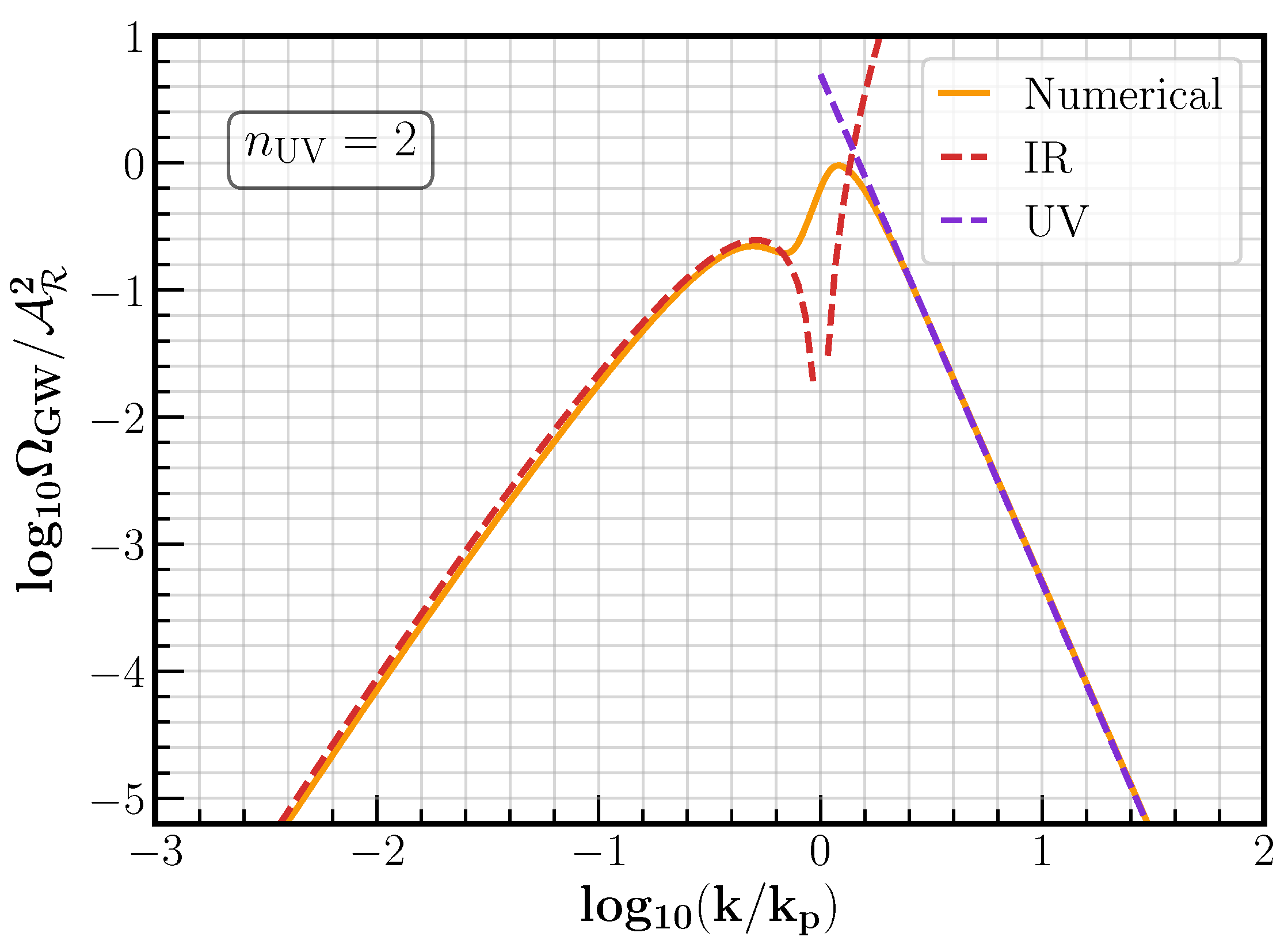
We later find that for there is a logarithmic correction [74]. Additionally, if the scalar spectrum of fluctuations is really a Dirac delta, the spectrum slope is given by due to the unphysical divergence of at . Note that for tensor modes which entered during the radiation domination era we have to match the first line of (20) to the subhorizon solution. This yields a spectral index given by
which is in agreement with the general results of Ref. [78]. These naive derivations will be later recovered from the analytical formulas in Section 4. It is interesting to see that for () the induced GW spectrum peaks at which is clearly different than the peak in the primordial spectrum at .
The intuitive physical picture behind (22) is the following. In a universe with constant b, modes of a massless field (e.g., the tensor modes or the scalar field ) which enter the horizon early get more diluted than modes which enter later. For example, consider that right after horizon crossing, i.e., when , we have that the energy density of the massless field starts to dilute as . Since we have that then and . Thus, if the IR tail of induced GWs in radiation domination goes as , we expect due to dilution [78]. However, as we have shown, this is incomplete for induced GWs from a peaked spectrum. For , the density fraction of the scalar field grows as . This means that induced tensor modes which are generated later have a larger source and a larger amplitude than those generated earlier. In other words, for small k have a larger amplitude than large k by a factor . Then, for the density fraction of induced GWs goes as [74]. This gives the general formula that we derived in (22). Whether this absolute value of b is unique to induced GWs is something yet to explore.
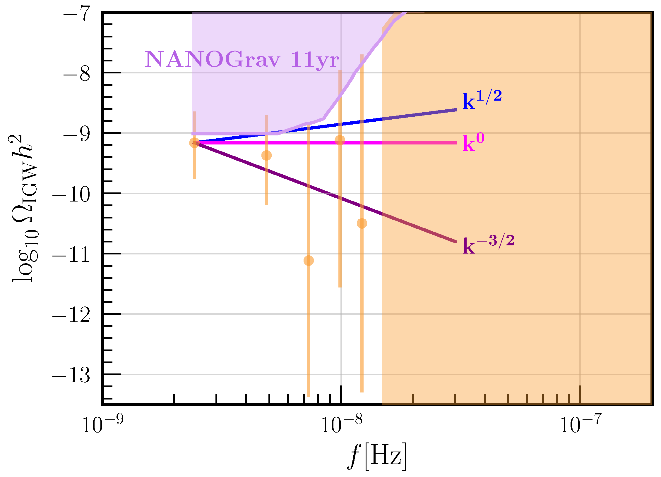
Before moving on to the near peak limit, let us comment on the implications of Equation (22). While the far most IR tail of the induced GW spectrum indeed must go as , we may have an intermediate regime where . This has interesting consequences when comparing with GWs from other sources. Let us model a general GW spectrum by a broken power-law around a characteristic scale , as done in Ref. [172]. Then, for example, the IR spectrum of induced GWs for () resembles that of GWs generated by a strong first order phase transition which have for and for . This gives another very good reason to be open about a primordial universe with a different equation of state than radiation.
2.2.2. The near Peak Regime
Looking closely at Equation (19), we might suspect that there could be a resonance if the wavenumber k of a tensor mode approaches that of twice the scalar mode . This resonance may be understood in two ways. First, we know that a harmonic oscillator with an external force has a resonance when the period of the force matches that of the harmonic oscillator. If that occurs, the amplitude of the oscillations diverges in time. In short, the external force is kicking the oscillator at the right times. The second way to see it is that two scalar modes with physical momentum have a preferred window to produce a tensor mode with physical momentum equal to twice the scalar momenta, i.e., , if allowed by momentum conservation. To see this mathematically, let us redefine the tensor modes in Equation (19) to remove the Hubble friction by
With this new variable Equation (19) now reads
where we only focused on the oscillatory behaviour of the scalar field for . The particular solution to can be found by the Green’s function method (see Appendix B for the details). Neglecting the term proportional to in Equation (25), the homogeneous solutions to are . With such homogeneous solutions, the particular solution by the Green’s method reads
We clearly see from the integrand in Equation (26) that there is a resonance when the frequency of the sine equals that of the exponential. Then the oscillations interfere and leave the integral of a power-law. Since we are only interested in how the amplitude diverges, let us only focus on the divergent part of (26) which is given by
We see that when the resonance is effective and the amplitude diverges. Note that for the divergence is logarithmic. When the resonance is not effective enough to cause a divergence as the amplitude of the integrand decays faster than . However, since we so far used a Taylor expansion around we expect that for Equation (27) still yields the leading contribution after the constant term. Thus, for we also expect a peak at around , albeit not divergent. For the situation is less clear and a detailed analysis is necessary. Nevertheless for , we can roughly write that the tensor modes in the near peak regime have an amplitude given by
This also implies that the induced GW spectrum has a peak near with a growth rate proportional to
These estimates will be later checked by the general analytical solutions in Section 4. Thus, the resonant peak in the induced GW spectrum has information on the sound horizon by the position of the peak and on the expansion history b by the growth rate around the peak. This type of resonant structure is characteristic of induced GWs. Thus, the observation of such resonant peak could give strong evidence for induced GWs. Then, the sound speed of fluctuations and the peak could be disentangled by the simultaneous observation of the PBH counterpart, which we proceed to discuss. Note that in (29) the radiation domination case is “special” because it is exactly when the amplitude of the source term is proportional to the background density.
2.3. Primordial Black Hole Counterpart
In this section we briefly introduce the PBH counterpart to the induced GWs. It is by no means a review on PBH formation and it does not intend to be so. A detailed review on PBHs can be found in Ref. [174]. Other interesting reviews are listed at the Section 1.2. PBHs from large primordial fluctuations will form in those Hubble patches where the density contrast is above a certain threshold8 [190,203,204,205,206,207,208], which depends on the EoS parameter w at horizon re-entry [209,210,211,212,213,214,215,216]. Since fluctuations generated during inflation closely follow a Gaussian distribution centred around zero, only the tail of the distribution has a large enough amplitude to collapse to PBH. This means that PBH formation is an extremely rare event. The fraction of Hubble patches where PBH forms is exponentially suppressed and sensitive to the root mean squared of the distribution, which is related to the power spectrum. This is why we generally need to form a substantial fraction of PBHs. Precise estimations of the fraction of PBH is an active and ongoing research field, e.g., see Refs. [202,214,215,216,217,218,219,220,221] and references therein. For our purposes, it is enough to know that only large induced GWs have a large associated fraction of PBH and, inversely, the absence of large induced GWs rules out PBHs from large primordial fluctuations.
For simplicity, we continue with the assumptions of the previous section and take a primordial spectrum with a Dirac delta peak at . This essentially leads to an almost monochromatic9 PBH mass function. When the peak in the scalar spectrum enters the horizon, those fluctuations which are above collapse into a PBH. By the end of the collapse, only a fraction of the total mass enclosed inside the horizon at horizon crossing () will end up as a PBH. We use the symbol ⊛ to refer to evaluation at PBH formation time. In mathematical terms, we have that PBHs mainly form with a mass equal to the mass enclosed inside the Hubble sphere, that is
To grasp the magnitude of the actual PBH mass, let us write it in terms of a solar mass by referring all quantities in (30) in terms of the size of the horizon at matter-radiation equality, which is very well measured by Planck [2]. The numerical factors and formulas used to derive this and the following estimates can be found Appendix A. After some numerical manipulations we arrive at
where we kept our ignorance on the primordial universe by leaving a free b (or w) (16). We took in a radiation dominated universe [206] but it may differ for different expansion histories [209,210,211,212]. and are the effective degrees of freedom in the energy density and entropy evaluated at reheating. It should be noted that we also assumed an instantaneous reheating. In that case, the horizon scale at reheating can be related to the reheating temperature by
As we have seen in Section 2.2, the peak in the primordial curvature power spectrum induces GWs. These GWs have a typical frequency associated to the wavenumber . Since the typical mass and the typical frequency are related by the same typical scale , we can write one in terms of the other. In this way, the typical frequency evaluated today reads
For a radiation dominated universe () we have a one-to-one correspondence between the frequency and the mass. If we fix the reheating scale, the relation (33) roughly tells us that PBH with a given mass have an induced GW counterpart with a peak frequency at around . The exact relation between and depends on the value of b. For instance, if () the expansion rate was faster and for a fixed corresponds to smaller PBH mass at formation. The opposite holds for (). It should also be noted that for () there is another peak in the induced GWs at . This may break the correspondence between the PBH mass and the peak of the induced GWs if not all of the GW spectrum is seen.
3. General Formalism
In this section we present the general formulation of induced GWs. This includes the derivation of the equations of motion in Section 3.1 and the general form of the solutions in Section 3.2. Then in Section 3.3 we include the leading terms due to local-type non-Gaussianity. In Section 3.1, we derive the equations of motion using the action formalism and so we do not follow the conventional derivation, e.g., of Refs. [35,38]. The final result is obviously the same, but the derivation is rather quick and clear. Throughout this section and on, we shall neglect the effect of vector perturbations as they typically decay. Anyone interested in the approximations and applications may jump directly to Section 4.
Main references: In Section 3.1 we closely follow Ref. [150] although we work at the level of the Lagrangian. For alternative derivations starting from the Einstein equations see for example Refs. [35,38,39]. Then, Section 3.2 is extracted from [64] which is built upon and uses the notation of Ref. [63] except for the numerical factor 2 involving . Lastly, Section 3.3 on the primordial non-Gaussianity is mainly based on Ref. [81] updated and corrected by Ref. [92].
3.1. Derivation from the Action
We need to arrive at the equations of motion for the transverse-traceless component of the spatial metric at the second order in cosmological perturbation theory. Although it is a second order calculation, we shall derive it quickly from the action formalism; if we work in a particular gauge and we only focus on the interaction of tensor with scalars. It is particularly convenient to work in a gauge similar to the Newtonian gauge10 with the exponential notation typical of Misner, Throne and Wheeler [184]. With this choice and assuming a perturbed FLRW universe, the metric reads
where is the metric of our space-time, are the spatial components, is the scale factor and we have further used the conformal decomposition of the spatial metric such that
Note that for a flat FLRW background in Cartesian coordinates we have . The conformal decomposition of the spatial metric is very convenient and simplifies calculations. It is also used, e.g., in Numerical Relativity [222]. In short, the conformal decomposition completely splits the trace (volume changing) from the trace-free (volume preserving) degrees of freedom. In the Newtonian gauge this decomposition directly splits the scalar and tensor modes of the spatial metric. This means that only contains the transverse-traceless degrees of freedom. As we shall see, it also leaves a clean splitting between and at the level of the action.
To consider a sensible cosmological set up, we include a canonical scalar field in the perturbed FLRW metric. We can later generalize it to a perfect fluid quite straightforwardly. The action, without any decomposition, is given by
where g is the determinant of , R is the 4D Ricci scalar, and is the potential of . In the (3 + 1) conformal decomposition (34), after some algebra and integration by parts, the action becomes
where and are respectively the 3D Ricci scalar and the covariant derivative associated to . Since we work in Cartesian coordinates, we already used that . In going from (36) to (37) we took a big leap in the (3 + 1) and conformal decomposition of the 4D Ricci scalar. Some steps can be found in Appendix C. For more details, the interested reader is referred to E. Poisson’s book [223] for the (3 + 1) or ADM decomposition [224], and to the appendix of R. Wald’s book [225] for the conformal transformation rules.
Now, we could take the variation of (37) with respect to , having in mind that the result should still be transverse and traceless, and obtain the transverse-traceless spatial component of Einstein Equations. However, this would not be very illuminating. Before taking the variation, let us use cosmological perturbation theory and expand the action. A smart way to decompose the spatial metric and to keep the requirement (35) is to take the exponential matrix, i.e.,
where are the transverse-traceless (tensor) modes and satisfy . This is used, e.g., in Maldacena’s work on non-gaussianities [226]. For the details of the expansion in general gauges see [150]. From now on, spatial indices are contracted with the background spatial metric , for example . The inverse metric is then . With this expansion, the 3D Ricci scalar up to second order is given by
We stopped at second order since we are only interested in scalar-scalar-tensor interactions. We split the other variables as
where is the background solution and , and are the perturbations. Using the perturbative expansions (38) and (40) and only selecting the terms with two scalars and one tensor, we arrive at
where the first two terms correspond to the second order Lagrangian of the tensor modes. By taking the variation with respect to we obtain the equations of motion of induced GWs, namely
where is the Hubble parameter and is the transverse-traceless projector, so that the equation is consistent with the transverse-traceless degrees of freedom. For the moment, it is enough to know that it satisfies the requirements of a transverse-traceless object for both pairs of indices. Also note that in the current case of study, we have no source of anisotropic stress. Thus, for the sake of simplicity and consistency, we momentarily cheat and use the traceless part of the spatial component of the linear Einstein equations in Appendix E, which in the absence of anisotropic stress yields
Note that this is not strictly true in the early universe where neutrinos have a large mean free path and give a tiny contribution to the anisotropic stress [39,40].
Before going to the general solutions of the induced GWs, let us translate the current calculation to the perfect fluid picture. A perfect fluid with energy density and pressure P is described by the following energy-momentum tensor:
where is the fluid 4-velocity. The perfect fluid is specified once the equation of state is given. In the perturbative expansion, one takes and where v is the velocity perturbation and we neglected vector modes. The energy momentum tensor (44) has to be compared with the one for the scalar field, which reads
The perfect fluid description of the scalar field follows from the identification
If we simply focus on the spatial component we find that
Thus, in terms of the perfect fluid description we have that
This result coincides with the equations derived in Ref. [38,39]. Note that Equation (48) will slightly change in the case of a multi-perfect fluid system. We expect contributions from the relative velocities of the fluids. For a radiation-matter dominated universe, the source term to induced GWs can be found, e.g., in Ref. [70].
3.2. General Solutions
To solve for the induced GWs, we must solve beforehand the first order equations of motion. Continuing with the scalar field fluctuations , we find that they are related by the momentum constraint to by [183]
Thus, we must only solve for the only scalar degree of freedom , which we will do briefly. For the moment, we take a general approach and split into an initial value and a transfer function as
If we are considering primordial fluctuations, the initial spectrum for is set on superhorizon scales () by quantum fluctuations during inflation. However, in general, any source of fluctuations to the curvature perturbation will lead to induced GWs. We will discuss this possibility later in Section 6. With Equations (49) and (50) we can formally solve the equations of motion for induced GWs [38,39], which in Fourier space read
with
and
where we wrote in terms of b using Equations (15) and (16). To derive Equation (51) from Equation (48), we used the Fourier transform for in terms of the polarization tensors which are defined in Appendix D. Then, we used that the projection of with the Fourier transform of the transverse-traceless projector is trivial, i.e., . Now, with the Green’s method we can find a formal solution to (51) given by
where is the Green’s function of the homogeneous solutions to (51) given in Appendix B. The formal solution (54) is defined such that at the initial time we have . Any GW with primordial origin, i.e., generated during inflation, may be simply added to the solution (54).
Since we are interested in the main observable of the SGWB, that is the GW power, let us compute the 2-point correlation function of the induced GWs which is given by
Here we have neglected any primordial signal but we could add one without further issue. In fact, this was considered in Ref. [88] where they may have a non-trivial cross-correlated spectrum by tensor-scalar-scalar couplings during inflation. We will not pursue this possibility further in this review. Continuing with Equation (55), we can compute the two-point function of the source term by
We see that the induced GW spectrum depends on the 4-point function of the scalar fluctuations. Such a 4-point function may be decomposed in general into a disconnected, i.e., the product of 2-point functions, and a connected piece [89]. If we consider that the stochastic fluctuations are drawn from a Gaussian distribution, the connected 4-point function vanishes and we are led to11
We discuss the case of mildly non-Gaussian fluctuations in Section 3.3. With further manipulations of Equations (55) and (8), integrating one internal momentum using a Dirac delta and writing the remaining integral in spherical (momentum) coordinates, we arrive at
where we followed the notation of Kohri and Terada [63]. In Equation (58) we already summed over polarizations (see Appendix D for the details) and we have introduced for convenience
We also took the oscillation average, i.e., we integrated over half period and divided by , to take into account that observations of the SGWB actually measure an average over many wavelengths. Furthermore, we have inserted all the time dependence into a “kernel” or “transfer function” defined by
The (averaged) power spectrum (58) is the main quantity needed for the calculations of induced GWs. Knowing (58) we can compute the spectral density of GWs by Equation (7). Note that the induced tensor power spectrum (58) is valid for any curvature perturbation regardless of its origin as long as it is Gaussian. In the next section, we discuss in more detail the case when the fluctuations are generated during inflation.
3.3. Inclusion of Primordial Non-Gaussianity
Primordial fluctuations generated out of quantum fluctuations during inflation are very close to being Gaussian, although not exactly. Small departures of a Gaussian distribution are expected due to gravitational interactions [183,226]. These perturbative departures from the Gaussian distribution are often referred to as Non-Gaussianity (NG).12 Depending on the formation mechanism, e.g., due to large interactions among fields, we may obtain some significant level of NG. The possibility of observing NG of primordial fluctuations is very exciting, as it might provide information on the particle content during inflation. For this reason, the study of NG is sometimes referred to as cosmological collider physics [227].
For practical convenience, the predictions of primordial fluctuations generated during inflation are often given in terms of the curvature perturbation . This is because is a non-linearly conserved quantity on superhorizon scales [228]. This makes it easy to set well-defined initial conditions on superhorizon scales for whatever scalar variable one might want to consider, independently of what happened previously (e.g., how inflation ended). For instance, since we are working in the Newtonian gauge, we have to relate with . It can be shown that on superhorizon scales the linear relation is given by [229]
In the case at hand, we are interested on NGs generated during inflation, i.e., primordial NG. These primordial NGs are often parametrized by the amplitude and shape of 3-point function or the bispectrum [180,181]. For simplicity, we usually consider only the local type NG which can be expressed as a local perturbative expansion around the Gaussian curvature perturbation by
where the factor is by convention.13 Note, however, that this is just a particular shape of the NG. Currently though, there is no study on the impact of other shapes of NG on the induced GW spectrum. Now, if we go to Fourier space the squared term in (62) becomes a convolution. Then, we can write that for the modes the perturbative expansion is given by
where to avoid unnecessary numerical factors we have introduced
We can then expand perturbatively the 4-point function in (56) as
The first term on the right hand side of (65) is already computed in Equation (57). If we focus on the second line in the NG contribution of (65), we see that there are 6 possible non-vanishing Wick contractions in the first 6 point function of which, together with the 4 remaining possibilities of the third line, makes 24 terms for the first NG contribution. In the fourth line of (65) there are 8 possible non-vanishing contractions, which make 16 possibilities counting the fifth line. The total is then 40 non-vanishing contractions.14 The NG contribution can be further classified into three different terms following the notation of Ref. [92]: the “H”, the “C”, the “Z”. Using Equation (65) in (8) and (55), these NG contributions to the induced tensor spectrum can be respectively written as
and
These derived formulas agree with those of Ref. [92]. We will assume that we are in the perturbative regime, so that the NG contributions (66) and (67) should be thought of as a correction to the Gaussian contribution (58). The first contribution (66) is also referred to as “hybrid” [90]. Additionally, note that the second line in (66) can be reabsorbed into a redefinition of the primordial power spectrum to include non-Gaussianities. For instance, we could write
which follows from the computation of using Equation (63). This is the term considered by Cai, Pi and Sasaki [89] and acts as a local redefinition of the primordial spectrum. With the form of Equation (69) it is much easier to compute the induced GW spectrum up to since it just accounts for a replacement of in (58) for .The second contribution (67) was first considered by Unal [90] and the third (68) by Ref. [81]. Unal also considered the terms of [90]. Most recently, Adshead, Lozanov and Weiner [92] presented a detailed and complete analysis of all the contributions up to . The interested reader is referred to Ref. [92] for the detailed formulas. We discuss the main features of the NG corrections in Section 5. It should be noted that the effect of primordial NG might compete with the terms due to non-linearities, e.g., from studied third order contributions to the source term of induced GWs. The reader is referred to Refs. [143,179] for the details on the third order expansion. Lastly, it should also be noted that for simplicity we assumed a scale invariant in (62). However, in general situations one expects that is scale dependent. For a recent study on the impact of the scale dependence see Ref. [93].
4. Analytical Transfer Functions
In general situations the kernel (60) and the power spectrum (58) have to be computed numerically. The problem is that the time integral in (60) is extremely demanding for , as the integrand is the product of three oscillating functions with frequencies that depend on the tensor and scalar mode wavenumbers. In fact, is the range of scales we are interested in. If we extend the integral until today, say at , and we look at scales much smaller than the horizon, we trivially have . However, there is more we can learn. For instance, scales accessible to future GW detectors range from to . These very small scales entered the horizon much before BBN, which roughly correspond to the time when modes with entered the horizon.15 Luckily, this implies that we can evaluate the kernel (60) some time prior to BBN when induced GWs are really inside the horizon and in a radiation dominated universe. Then, from that moment on, we may simply treat these induced GWs as a radiation fluid with . Note that we will also consider the case that the modes of interest enter the horizon in an epoch where . In that case, we must follow induced GWs until the universe transitions to the standard radiation dominated era. We will provide more details later.
Surprisingly, there are relevant regimes where the integrals in (60) can be done analytically. This is the case of a constant equation of state parameter w and constant propagation speed of fluctuations . For example, this includes a perfect fluid whether it is made of a scalar field16 or an adiabatic perfect fluid, which are commonly used in cosmology. Even when there are transitions between one perfect fluid domination to another, there will be periods in which w and are almost constant. Thus, the constant w and limit is a good approximation in a cosmological set up if the modes of interest enter the horizon outside the transition periods. With these assumptions, we present the solutions to first order cosmological perturbations in the Newtonian gauge in Section 4.1 and derive a very simple form of the source term (53) for the induced GWs. In the general situation where , the integral (60) can be analytically done for modes which either enter the horizon before or after the transition. In this way, in Section 4.2 and Section 4.3 we respectively derive the kernel for modes which are subhorizon and superhorizon before the transition. When then follow our solutions to the radiation dominated epoch.
Main references: The whole section is a generalisation of Refs. [64,74] to account for not only general constant w but general constant . The notation used here improves and unifies those of [64,74]. The main base of Refs. [64,74] was started in [39,63] in the radiation dominated universe.
4.1. First Order Solutions
At the moment, the formal solution (54) for the induced tensor modes does not tell us much. To extract some meaningful information, we have to solve the equations of motion for first order perturbations, which are given in detail in Appendix E. After some simplifications, the equation for the Newtonian potential for general w and and in the absence of isocurvature17 fluctuations reads18
where we have also introduced as in Equation (15) as well as
The notation , and s is typical of inflationary models and simplifies the form of the equations. One may of course write Equation (70) in a more conventional notation, e.g., that in Mukhanov’s book [229] which for constant reads
where and . In the case of an adiabatic perfect fluid one has . In the case of a canonical scalar field we have and . As we already mentioned, for analytical viability we are mostly interested in the case of constant w and . This requirement in turn implies , so that the Newtonian potential in Equation (70) behaves as a massless field. The solution to (70) for general and w is given in terms of Bessel functions of the first and second kind, explicitly
where b in terms of w is defined in Equation (16). Now, we must give some kind of initial conditions to . If the primordial spectrum was generated by quantum fluctuations during inflation, the initial conditions are well-defined and constant on super(sound)horizon scales, that is when . By picking up the asymptotically constant term in (73), we find that and
where is the primordial (stochastic) value set by inflation. Note that the general solution (73) is not valid for where the gradient term in (70) is absent. Nevertheless, the solution for constant w is just on all scales. The case of is quite particular as the fact that does not decay implies a constant source to induced GWs. This makes the detailed dynamics of the transition to radiation domination very important for the final GW spectrum [65,66], when the source term experiences drastic changes. We dedicate Section 6 to this particular case.
With an exact analytical formula for the first order perturbations, we can attempt to compute the resulting induced GWs. For that, we first need to know the two independent homogeneous solutions to the tensor mode Equation (51), say and . For constant w they are given as well in terms of Bessel functions with one order less than in , concretely
In Equation (75), and respectively are the growing and decaying modes. Note that there is no since in general relativity tensor modes propagate at the speed of light. This yields a Green’s function (see Appendix B) given by
This finishes the list of necessary ingredients for our induced GWs calculations. In passing, since there always appears the combination or we introduce the useful notation
which we will use from now on. Additionally, a tilde on x implies a tilde on , i.e., .
Thus far it seems that we may have to deal with several integrals containing at least three Bessel functions, which is challenging to do analytically in general. However, the source term to the induced GWs ends up acquiring a simple enough form after several simplifications. For instance, using the Bessel functions properties (see Appendix F), we find that Equation (53) reduces to
where we used x from (77) and u and v from (59). To arrive at (78) one needs to write the Bessel function that appears in in a combination of and which can be found in Appendix F. So far, it is not entirely clear whether there is any physical reason behind the simplification (78) which turns out to render the source term as a sum of the squared of Bessel functions of the same order. This simple form of the source term is crucial to obtain analytical formulas for general b and that we derive below.
Replacing (77) and (78) into Equation (60) we find that the kernel can be written as
where we defined for compactness
Unfortunately, we are not aware of a general analytical formula for the time integrals (80) unless , in which case the Bessel functions reduce to spherical Bessel functions and can be written in terms of transcendental functions. This is for example the case of radiation domination (), where the general kernel can be found in Ref. [63]. Nevertheless, we can integrate (80) in two relevant limits, (subhorizon) and (superhorizon).
Let us explain the assumptions needed for the approximations before jumping into the actual calculations. We are considering that right after inflation there is a period when the universe has a free b (or w) and free . However, to recover the standard hot big bang cosmology, such an epoch must end, and the universe must enter a radiation domination stage. Thus, whatever solution we find in this section for the induced GWs must be followed until we reach the radiation dominated stage. For simplicity, we will assume an instantaneous transition. Then, we will refer to the time of transition as “reheating” time and the comoving size of the horizon at that time as “reheating” scale . The value of in terms of the “reheating” temperature can be found in Equation (32). The assumption of an instantaneous transition might be important for those tensor modes with wavenumber . Namely, those modes which entered the horizon around the transition. If the transition is gradual, then our approximations will not be very good for modes which entered during the last stages of the transition. In any case, as we shall see, the instantaneous approximation gives a very good idea of the shape of the induced GW spectrum even for . On top of that, we will assume that the scale corresponding to the peak of the primordial spectrum enters the horizon well before reheating so that during and after reheating there is no significant source of induced GWs. In the case of a top-hat primordial spectrum, this means that the scale corresponding to the IR cut-off enters the horizon much before reheating. Under these two assumptions, i.e., sudden transition and “localized” primordial spectrum, we can proceed to derive our analytical formulas. Note that this does not apply to the case when which we discuss in Section 6.
4.2. General Subhorizon Kernel
Let us start with the simplest situation. This corresponds to the case when all modes of interest entered the horizon much before reheating, that is . Then, we can safely send the upper integration limit in (80) to infinity, i.e., . This is because when we eventually match our solution at reheating to a free GW propagating in a radiation dominated universe, the upper limit would be . The integrals (80) for are derived by Gervois and Navelet [233] and given in Appendix G. Here we just give the form of (79) after integration, which reads
where is the Heaviside function, and are the Ferrer’s function of the first and second kind, valid for , and is the associated Legendre function of the second kind, valid for . Their explicit expressions in terms of Hypergeometric functions can be found in Appendix H. We also defined for simplicity
and we Taylor expanded the Bessel functions for large argument. Note that y is related to the area of the triangle made by the three momenta, , and k. The presence of the Heaviside function in (81) signals the possible resonance we anticipated in Section 2.2 when the wavenumber of a tensor modes equals the sum of two typical scalar modes . In more practical terms, when the three Bessel functions in the definite integral (80) for conspire (by rendering their product as coherent oscillations) and yield a divergent integral. Additionally, note that Equation (81) has the same time dependence as a subhorizon tensor mode propagating in a constant b and universe, e.g., see Equation (75). In other words, it decays as and oscillates with a frequency proportional to x. This was expected as the source term for induced GWs decays once inside the horizon and, therefore, induced GWs behave as a freely propagating GW. This does not apply in the case of a dust dominated universe though.
In the current form Equation (81) is general enough so that it can also be used in the C (67) and Z (68) NG terms. However, in this review we are more interested with the Gaussian contribution (58). Thus, we are more concerned about the averaged square kernel. After some simple algebra, that is squaring (81) and calculating the oscillation average, we arrive at
With the averaged kernel (83) we are ready to compute the induced GWs in quite general situations. We are only left with the integral over momenta which can be easily computed numerically. Analytical formulas for the final GW spectrum are discussed in Section 5. Let us note that although (83) might look technically complicated to implement, it is by far more useful than attempting a numerical integration of three Bessel functions. Furthermore, the superhorizon approximation is very good for modes with regardless of the shape of the primordial spectrum. This is because induced GWs with are essentially already free GWs. Thus, soon after horizon re-entry and thereon they will behave as relativistic particles in an expanding universe. This also means that we can evaluate (7) and (83) at the instantaneous reheating time, i.e., , to estimate the observable spectral density of induced GWs. We will do this shortly. If the transition is gradual, the kernel (83) is a good approximation for modes which enter during a period with almost constant b.
In the next subsections, we will have a closer inspection to the kernel (83). After matching to radiation domination, we will look at the behaviour of the kernel near the resonant point and in the IR tail.
4.2.1. Matching to Radiation Domination
Let us discuss the matching to radiation domination in more technical terms. After matching the background quantities at , that is the scale factor a and the Hubble parameter we find that a and in the radiation dominated period follows the typical solution (found in (16) with ) with a shifted conformal time, which reads
where b is related to the equation of state of the previous epoch by (16). Now, for the matching of tensor modes it is important to realize that the continuity of and its first derivative imply the continuity of the kernel (60) and its first derivative. Thus, from now on we simply deal with the matching of the kernel (60). Since we are dealing with subhorizon scales we have that the kernel before the transition is
where the coefficients, not important at the moment, can be extracted from Equation (81). The kernel after the transition is also for subhorizon modes, which must have the form of a freely propagating GW in a radiation dominated universe, namely
This implies that although we should be calculating
with
it is equivalent to evaluate
with
where the kernel is that given in (83).
It is important to note that our subhorizon approximation is valid for modes with . Later, we may try to join the subhorizon approximation with the superhorizon approximation valid for by extrapolating up to . Let us call such scale . However, there is an important subtlety in joining the two approximations. If we look at the scale that last crossed the horizon at reheating, namely
we see that if we compare with we have that
For we have that . This means that our subhorizon approximation is even valid for and, therefore, we expect a good matching with the superhorizon approximation at (since for the modes are superhorizon before the transition). However, for we find . This time the subhorizon approximation breaks down for and so we expect the matching with the superhorizon approximation to be at . This is what we eventually find in Section 4. In addition to the above, we have that the subhorizon approximation has corrections of [74]. So for the corrections quickly become important for . A detailed studied for , perhaps with numerical methods, is needed to clarify the exact shape of the GW spectrum. Nevertheless, our results should be a good order of magnitude estimate.
4.2.2. Resonances
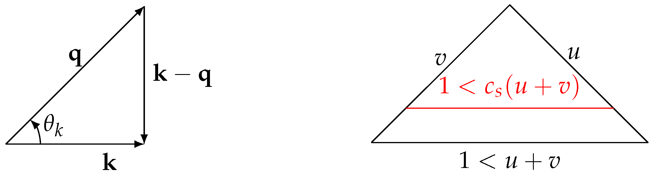
Here we focus on the general behaviour near the resonant point for the averaged kernel (83) that we discussed in Section 2.2. We start by noting that we have three vectors, the one from the tensor mode and the two scalar modes, and , which of course satisfy momentum conservation. Recall that from Equation (59) q corresponds to v and to u. This means that our three variables satisfy a triangle inequality, that is
which translates into
The area A of the triangle made by k, q and is related to the angle between and by
This means that the projection with the polarization tensor (see Appendix D) is proportional to the area, namely
This implies that the saturation of the triangle inequality at corresponds to zero area and, therefore, does not contribute to the integral (58). Now, from the arguments in Section 2.2 we expect a resonance when
Thus, if we have the resonant point coincides with the saturation of the triangle inequality and, thus, has vanishing contribution. In this way we see that, by momentum conservation, there is no resonance for in the induced GW spectrum. Nevertheless, for we do have a resonance inside the integration region (see Figure 2).
We can confirm these expectations by expanding the kernel (83) around which corresponds to , where the associated Legendre functions might have a divergence. The asymptotic behaviours around are given in Appendix H. Focusing first on the case , we find that the kernel diverges as
This recovers Equation (29) which showed that a very peaked primordial spectrum, so that , leads to
The case is explicitly given in Equation (209). In the case when , we arrive at
which is independent of y. Thus, as expected there is no resonance for . Nevertheless, as shown in [64] for there is still a peak at in the induced GWs spectrum for a peaked primordial spectrum. We can roughly understand the peak by noting that since , the next leading order must be since . Then, inserting this into the kernel (83) we find that
For and there is no detailed study of the kernel (83). Nevertheless, by looking at the explicit expression for (213) we see that there is nothing special at . Before ending this section, note that the kernel is symmetric around the resonant point . It displays the same behaviour when approaching from both directions, .
4.2.3. Infrared Regime
Here we show the behaviour of the kernel when which is the relevant regime for the IR tail of the GW spectrum as and . This limit means that, if there is any peak in the spectrum of scalar fluctuations, we are looking at scales much larger than the scale of the peak. Thus, such limit of the kernel (83) is relevant for wavenumbers , where we included since it is the limit of the subhorizon approximation. The cases and exhibit different behaviours as anticipated in Section 2.2. In the limit , the average kernel (83) is respectively given by
for and
for . They are actually very similar to (100) and (102), except for the fact that we are now looking at , so that . Evaluating (104) and (105) at the time of reheating and taking into account the factor in (58), we see that whatever the IR scaling in the radiation dominated universe (which for localized sources is [78]) we have to correct the exponent by a factor , i.e., to for a localized sourced. This is the same result as in Section 2.2. The absolute value is due to an extended superhorizon growth of tensor modes for , as explained in Section 2.2.
4.3. Superhorizon Kernel Approximation
In the previous subsections we have studied in detail the subhorizon kernel. However, there are modes which are still superhorizon at the time of reheating. Thus, for such modes we cannot take the upper limit in (80) to as at reheating. In addition to the approximation , we will use the assumption that the peak in the scalar spectrum is on scales . This means that we are only concerned with the region of integration of (80) around the peak in , where we have that and therefore . Using this fact we can expand the first Bessel function for a small argument in (80) and integrate in the limit of . By doing so we arrive at Equation (20) but for the kernel, namely
where the exact coefficients are given by
The details on the integrations can be found in Appendix G. Thus, we have found the kernel for modes which are superhorizon before reheating. However, these induced tensor modes are not yet GWs so we must follow them after they enter the horizon in the radiation domination era.
Matching to Radiation Domination
The kernel (106) is valid for superhorizon modes during an arbitrary period. After this period ends with a sudden reheating, we shall assume that the source term is shut off and tensor modes evolve as freely propagating massless tensor mode. As explained in Section 4.3 the continuity of implies continuity of the kernel. This means that the kernel goes from (106) to the kernel of a superhorizon tensor mode in radiation domination, which reads
where we introduced from the continuity of the background FLRW metric, i.e., we imposed continuity of a and at . Matching (108) and its first derivatives with (106), we find that
Thus, we have effectively continued the superhorizon kernel from the era to the radiation era. We can now follow the kernel down to subhorizon scales, which must behave as a tensor mode in a radiation dominated universe as there is no source, that is Equation (75) with . Then, taking the averaged square kernel yields
After picking up the most relevant contributions, that is the leading terms for , we arrive at
This is the kernel squared that should be used in the induced GW spectrum (58) for scales . In this way, the kernel (111) yields the right IR scaling for localized sources in a radiation dominated universe, i.e., [78]. The matching between the superhozion (111) and subhorizon (83) approximations at has shown to be very good in the instantaneous reheating case [74]. Note that for a gradual transition, the superhorizon approximation should still be good enough except for those modes which enter during the transition. We can then calculate the spectral density of induced GWs by
with
and using Equation (111). Nevertheless, it is worth noting that for a Dirac delta or a fairly sharp peak and a good approximation to the full induced GW spectrum is to stop the subhorizon spectral density (90) at and match with a power-law [74]. The amplitude of can be found by matching the two.
It should be noted that Equation (111) does not recover the logarithmic correction typical of induced GWs in a radiation dominated universe [79]. The main reason is that we assumed the source term to stop at reheating and, therefore, that superhorizon tensor modes at that time behave as free tensor modes. This is a good approximation taken for simplicity. However, the precise matching would require to first match the Newtonian potential from a universe to radiation domination and then continue the kernel (60) after reheating with the matched . This would give a more accurate calculation and would most likely recover the logarithmic correction in the IR tail.
5. Typical Induced GW Spectra
In Section 4 we derived analytical approximations for the kernel (or transfer functions) of induced GWs. However, we still have the integral over the scalar momenta. While the kernel was not so sensitive to the shape of the primordial spectrum, i.e., the approximation is valid as long as all the relevant primordial spectrum enters the horizon before reheating, the integral over momenta crucially depends on the shape of the primordial spectrum. In this section, we will present the final form of the induced GW spectrum and discuss their main features. We will not be so concerned in the series of approximations to achieve analytical formulas of the GW spectrum, which can be found in the papers. Before doing so, we will carefully derive in Section 5.1 what is the spectral density of induced GWs measured today. Then we will focus on the simplest types of motivated primordial spectra. These are a very sharp peak Section 5.2, a log-normal peak Section 5.3, a broken power-law Section 5.4 and a scale invariant spectrum Section 5.4.2. We will also comment on possible oscillatory features Section 5.5 on top of the basic shapes and the impact of primordial NG on the final GW spectrum Section 5.6.
Main references: Although there are many studies on the induced GW spectrum for various primordial spectra, we focus on the cases where analytical formulas have been derived. In this way, Section 5.1 can be derived using the formulas in Appendix A and can also be found in [64,74]. Section 5.2 is mainly based on [74]. Section 5.3 follows [74,82]. Then, Section 5.4 is based on [81]. Section 5.5 briefly describes the results of Refs. [84,87]. Lastly, Section 5.6 reports the main findings from Refs. [89,90,92].
5.1. The GW Spectral Density Today
To find the power of GWs that we would observe we have to evaluate (7) today, namely
However, our computations in Section 4 were done up to and including the transition to a radiation dominated universe. Since deep inside the horizon we have that then after reheating we have that . To relate with we can make use of the fact that GWs behave as radiation and write
where is the density fraction of radiation today given by Planck [2]. We also traced and back to the reheating time taking into account that the effective degrees of freedom change with temperature. In the case that the induced GWs are generated during a radiation domination era we should replace the subscript “rh” for the evaluation at a time when the induced tensor modes start to behave as a GW. This is denoted with a subscript “c” by Inomata et al. [126].
5.2. Dirac Delta Peak
The simplest case is that of a very sharp peak in the primordial spectrum. While this type of spectrum is not possible to generate during single field inflation [103,109,234], it may be achieved in multi-field models of inflation [95,235,236,237,238,239,240,241,243]. If the peak is extremely sharp, it is often modelled by a Dirac delta as
Although this might be an unrealistic situation, it captures the essence of sharp peaks and gives insight on the kernel. We discuss a more realistic situation in Section 5.3. Now, for the power spectrum inside the integral (58) we have
and similarly for u. Recall, however, that the integral over u is bounded by momentum conservation to . So, when we integrate over v and u using the Dirac delta, the range is now . This translates to a range in k given by . After taking this finite range of k into consideration, we may simply evaluate at the integrand (89) (and (113)) and insert it into (88) (and (112)) to arrive at
Note that we are being general by allowing a phase before the standard radiation domination. Since we are assuming an instantaneous transition at from the to radiation domination, we have to include the scale corresponding to the last scale that entered the horizon at the transition. In more detail, is related to by
Thus, we have that . If we are considering the induced GWs in a radiation dominated universe we may simply replace and recover the standard formula [63]. In Figure 3 and Figure 4 we see the GW spectrum for different values of b and respectively for and , so that the resonance is evident.
Despite the fact that (118) is already a completely analytical formula, the functional complication does not provide much insight yet. Nevertheless, we can check one interesting limit, which is the IR tail of the spectrum. Expanding (118) for we arrive at a general analytical approximation for the low frequency tail of the GW spectrum. First, for we have that
where we set the broken power-law knee at since it is when the subhorizon approximation breaks down for . A more detailed discussion can be found in Section 4.2. Second, for we find
where this time the matching is roughly at . The above formulas agree with those in Ref. [74]. The difference between and is the continued superhorizon growth in the case of which is explained in Section 2. The most important aspect of Equations (120) and (121) is that it clearly shows how the IR spectral tilt of the induced GW spectrum is directly related to the equation of state parameter at the time of induced GW generation. Thus, the observation of the IR tail gives insight on the expansion history of the primordial universe. Interestingly, for () the spectrum has a peak at which is larger than that at . This means that induced GWs for peaks at a different scale than the peak of the primordial spectrum. This has been used, e.g., in [132] to fit the NANOGrav results [18] and at the same time predict PBH with a mass smaller than the solar mass. If instead one assumes induced GWs in radiation domination to fit the NANOGrav frequency range, the associated PBH counterpart must be of the order of solar mass. We discuss more about these possibilities in Section 9. Another important point is that the amplitude of the spectrum at strongly depends on the ratio and often mildly on b. We thus see that the smaller the ratio , the more suppressed is the spectrum at . This is because the main induced GW generation occurs when the scalar mode enters the horizon. Then, since the modes with have been superhorizon until the transition they can only grow by a factor . For the argument is slightly different because of the second superhorizon growth and so the suppression is minor compared to with a power index that depends on b.
5.3. Log-Normal Peak
We now turn to a more realistic situation where the peak in the primordial spectrum has a finite width. Inspired by several models of multi-field inflation the peak of the primordial spectrum may be parametrized by a log-normal [82], namely
where is the dimensionless width of the peak. Note that the power spectrum (122) is normalized, i.e., . The log-normal parametrization includes sharp peaks where [95,235,236,237,238,239,240,241,242,243] and broad peaks where [62,85,102,128,238,244,245,246,247,248,249,250,251,252,253,254,255]. For we recover the Dirac delta case.
In this review we are mainly interested in the case of a narrow peak (). The reasons are its simplicity and that we can use our results for general b of Section 5.2. The interested reader for analytical approximation in the broad peak case () in radiation domination is referred to the work of Pi and Sasaki [82]. Here we may directly borrow their result for which reads
where is the error function and is the GW spectrum induced by a -function peak given in Section 5.2. Then, Equation (123) provides the correction to the Dirac delta spectrum of Section 5.2 due to the small but finite width of the spectrum which leads to the IR scaling in radiation domination [78]. The most important effect then appears when the ratio of scales is smaller than the width . Indeed, when we have that
which gives a correction of when . Thus, due to the presence of our IR tail of Section 5.2 changes respectively for and to
or
Note that since the case still allows for a very sharp peak with . See how the inclusion of the finite width increases the richness of the induced GWs spectrum. We illustrate this in Figure 5. Additionally, note that if then the induced GW spectrum only has two different slopes and becomes meaningless.
Before ending this subsection, we briefly discuss the case when . It is shown in Ref. [82] that in the induced GW spectrum in radiation domination for and near is well approximated by
This means that the GW spectrum induced by a log-normal peak in the primordial spectrum also follows a log-normal peak but with a shallower width given by . The factor 2 is a reflection of the secondary nature of induced GWs [82].
5.4. Broken Power-Law
In Section 5.3 we have studied the log-normal sharp peak which is inspired in multi-field models of inflation. However, if the curvature perturbation is enhanced during single field inflation it often takes a broken power-law shape [103,109,234,256]. The induced GWs counterpart for a broken power-law primordial spectrum have been studied in Refs. [80,81,105,141,220]. Here we present the results of Ref. [81], which contain analytical approximations for the amplitude and spectral tilt of both the IR and UV tails of the induced GW spectrum. A detailed discussion on the approximations used can be found in [81]. At the end of this subsection, we also briefly discuss the case of a scale invariant primordial spectrum.
Let us parametrize the primordial curvature power spectrum as a strict broken power-law given by
where respectively are the IR and UV spectral tilts of the spectrum which peaks at . In single field models one often finds that [103]. If the enhancement of the curvature fluctuations is due to a bump in the inflationary potential, then can be related to the second derivative of the potential at the bump [80,256]. In such models is also related to the local non-gaussianity parameter [256]. In what follows, we will only focus on induced GWs in the radiation dominated universe and later discuss its generalisations to other values of the equation of state parameter. Currently, only analytical approximations for radiation domination are available. Now, using (91) and (128) we can compute the associated induced GW spectrum. Doing so for the IR tail, i.e., for modes with , we find that
Equation (129) is valid for and and gives a good approximation of the IR tail. The condition comes from requiring convergence of the integral at large internal momenta ().
The UV tail of the induced GW spectrum presents two different behaviours. If the integral converges even in the strict limit . This means that we can pull out of the integral (91) all the k dependence in and have that . The remaining piece is just a numerical factor. In this way, we find that the induced GW spectrum in the UV reads
where , for , is given by
and converges everywhere. The range of for which this approximation is valid depends on the value of b. We discuss this after presenting the results for radiation domination (). Since (131) has to be computed numerically, we present here a numerical fit for , which reads
The form of (132) has been found noting that the integral diverges in the exact limit . After several trial and error attempts, a reasonable fit was found to be (132). A detailed study of (131) might yield better analytical insights than (132). For the moment Equation (132) gives a good order of magnitude estimate. Note that when the induced GW spectrum present a logarithmic divergence [80,81]. Lastly, for the primordial spectrum has a sharp decay and, in analogy with the sharp peak, we do not expect that . Instead, there should be a fast fall off at around by momentum conservation. Indeed when we find that
We show the analytical estimates against the numerical results in Figure 6. See how even if the approximations are extrapolated to they still yield a sensible order of magnitude estimate of the induced GW spectrum.
With the above analytical estimates for the amplitude and the spectral tilt in the IR and UV limits we conclude that the induced GW spectrum has the following broken power-law shape
Equation (134) tells us that the UV spectral tilt of the induced GW has information the UV tail of the primordial power spectrum. This is to be contrasted with the IR spectral tilt, which does not tell us much about the inflationary model unless we measure the amplitude very well. Lastly, if we focus on the UV tail of the induced GW spectrum (134), we see that for example it may be degenerate with the GW spectrum from the sound waves in a first order phase transition [172].
5.4.1. Alternative Expansion Histories
Here we briefly present the spectral tilts of the induced GW spectrum if instead of radiation the universe was dominated by another perfect fluid. In this case, we find that (134) changes to [81]
where b is defined in Equation (16) and this time
Previously, in Section 2.2 and Section 4, we derived the IR broken power-law behaviour of the induced GW spectrum for general equation of state parameter. Now, in this section we have a power-law UV tail in the induced GW coming from the UV tail of the primordial spectrum. The additional factor with respect to (134) in the UV tail can be understood as follows. All modes with entered the horizon deep inside the era and before the scalar peak at . After that the induced tensor modes effectively behave as free GWs irrespective of whether or . Thus, the free GWs experience the typical relative redshift with respect to the background, which is the factor . Note that if the UV tail might have a blue tilt.
5.4.2. Scale Invariant Spectrum
A limiting case of the broken power-law studied (128), setting , is a scale invariant spectrum typical of slow-roll inflation. In this case, it is easy to convince ourselves that the induced GW spectrum for general expansion histories is given by
where
and is given by (83). Another explicit formula can be found at the summary Section 10. The integral (138) converges everywhere for any value of b and . However, note that (138) with (83) is only valid for . Nevertheless, since deep inside the radiation domination we expect a scale invariant induced GW spectrum it is reasonable to assume that for scales we can match the behaviour to the constant spectral density. A more detailed, perhaps numerical, analysis is needed to determine the spectrum for as induced GWs are being sourced before and after the transition.
5.5. Oscillatory Features
In the subsections above we have discussed the GWs induced by the simplest shapes of the primordial spectrum, that is a log-normal peak and a broken power-law. However, in some situations, it is expected that the primordial power spectrum presents a series of oscillations usually referred to as “primordial features”. For recent reviews on such features see, e.g., [257,258,259]. These oscillations can be classified according to the k dependence in their frequency. If the frequency is linear in k, the oscillations resulted from sharp dynamics during inflation. For example, a step in the potential in single field inflation [260,261,262,263,264,265,266,267] or a sharp turn in field space [84,86,254,255,268,269,270]. This case is also known as a sharp feature. If the frequency is logarithmic in k, the oscillations are called resonant features. They are due to resonances during inflation on subhorizon scales. For instance, resonances occur if the potential in single field inflation has wiggles or a massive scalar field is oscillating at the bottom of the potential [87,170,271,272,273,274,275,276,277]. In more general cases, such as general interactions [278,279] or alternative scenarios to inflation [280], the frequency of the oscillations in the primordial spectrum could be a power-law of k.
Remarkably, despite the induced GWs being a second order effect, oscillations are not completely washed out. The main difficulty is to derive analytical approximations to the induced GW spectrum. In this respect, Fumagalli, Renaux-Petel and Witkowski [84,87] and also Braglia, Chen and Hazra [86] did a detailed numerical analysis of the induced GW spectrum and derived motivated semi-analytical templates. Perhaps the most interesting case is when the oscillations in the primordial spectrum are . For example, this is the case when a sharp feature is responsible for the peak in the primordial spectrum [84,255]. Now, if the oscillations are large and separated linearly in k, we can gain intuition by looking at the sum of Dirac delta peaks [83,84]. In this case if we call to the frequency of the Dirac delta peaks in the primordial spectrum, then the frequency in the induced GW spectrum is [83,84] (in radiation domination ). Interestingly, in the more realistic situation studied [84] the induced GW spectrum follows an envelope as if there were no oscillations and, on top of that, oscillations appear near the resonant peak at and reach at most an amplitude of about in radiation domination [84]. We illustrate this possibility in Figure 7. Another example are oscillations due to a resonant feature in the primordial spectrum. In this case, if we call the frequency of the resonant feature, the resulting induced GW spectrum exhibits two oscillatory components with frequencies and . The relative amplitude of such components depend on both the frequency and the envelope of the primordial spectrum [87]. For the analytical templates and a more detailed discussion, see Refs. [84,87].
5.6. Impact of Non-Gaussianities
Here we briefly discuss the effects that primordial non-gaussianities may have on the induced GW spectrum. We will not dwell on the details, which are well explained in Refs. [89,90,92]. The leading formulas for local-type non-gaussianity can be found in Section 3.3. We describe the main effects of local-type non-gaussianity below.
First, let us focus on the very sharp peaks of Section 5.2 and Section 5.3. In this case, the most relevant effect is that the induced GW spectrum does not stop at but continues until . This is roughly because when including primordial non-gaussianity, the source term to induced GWs has three scalars. Thus, we have a cut-off at by momentum conservation. Note that this effect is characteristic of the sharp peak in the primordial spectrum. For large non-gaussianity, that is in Equation (63), the spectrum does not have the clear resonant peak of Section 5.2 but presents a few peaks with similar amplitude instead [89,92]. Second, in the case where the peak is broad or a broken power-law, the non-gaussian contribution typically has the same IR and UV spectral tilts [81,92]. For large enough , the induced GW spectrum also shows an additional peak/bump at around . If the non-gaussianity is large enough, i.e., , the non-gaussian contribution starts to dominate over the gaussian one [89,92]. However, it is not so clear whether one can achieve in inflationary models as in this case the non-gaussian expression (63) cannot be regarded as a perturbative expansion [81]. A more detailed and general analysis is necessary. It should be noted that if we include third order perturbation theory terms, the induced GW spectrum for a Dirac delta peak has three resonant peaks instead of one [143,179].
The primordial non-gaussian contribution to the induced GW spectrum, as we have just presented it, might not yield much information on inflation. For example, one may design a gaussian primordial spectrum such that the resulting induced GW spectrum is exactly as that of a primordial log-normal peak with large non-gaussianities. Although this may be a very complicated task, it is in principle possible. In this sense, there is no telling primordial non-gaussianity apart just from the induced GW spectrum [179]. Nevertheless, the story becomes more interesting when considering the PBH counterpart. Since PBH formation is highly dependent on the tail of the distribution of primordial fluctuations, any tiny deviation from a normal distribution could have an exponential impact on the fraction of PBHs. For the details see the recent discussions in Refs. [217,219,220,221,256,281,282,283,284]. Then, ideally one may use the two observations, the PBH mass function and the induced GW counterpart, to perhaps disentangle the primordial non-gaussianity from the primordial spectrum.
6. The Dust Dominated Universe
In previous sections we have derived intuitive and analytical formulas for the spectrum of induced GWs under the assumption that the universe was not dominated by a pressure-less perfect fluid with vanishing propagation speed of fluctuations, i.e., , so-called dust. The particularity of a dust dominated universe is that the Newtonian potential is constant on all scales. As can be seen from Equation (70) with , is a solution. This also implies that density fluctuations of the dust fluid grow. In fact, they grow as . This is the typical behaviour of a CDM dominated universe. This also means that there is a scale below which density fluctuations grow so much that they become non-linear, i.e., larger than . This occurs for modes with [51]
Note that it does not mean that if there are fluctuations on there will be no production of induced GWs. It means that we cannot completely trust our calculations since non-linear dynamics might be important, e.g., due to GWs from mergers. Nevertheless, we quite often have and thus perturbation theory for is sensible.
In Section 6.1 we show and discuss the subtleties of the dust dominated universe and derive analytical estimates for the amplitude of induced GWs in the case of an instantaneous transition. We apply our results to PBH dominated epoch in Section 6.2 and use overproduction of induced GWs to place stringent constraints on the scenario.
Main references: Section 6.1 is based on Inomata et al. [65,66] with the notation of Refs. [70,71]. These works are built upon previous papers by Assadullahi and Wands [51] and Kohri and Terada [63]. Then, Section 6.2 follows the pioneering work by Papanikolau, Vennin and Langlois [69] further extended by [70] to account for the transition to radiation domination. Lastly, Ref. [68] contains useful details on the transition of the PBH dominated universe to radiation domination.
6.1. General Dust Domination
Let us now derive the kernels and some estimates for the induced GWs. First we note that the fact that in an early Matter Dominated (eMD) era seemingly makes naive calculations of induced GWs easier. Just take a transfer function equal to unity in (53), which yields
where we took (). Now we have to simply integrate (60) with a constant source. In the limit where , we have that the averaged kernel squared is just a constant [51,63]. In our notation we have
We can then use (58) to give a naive estimation of the induced GW during the early matter era. However, this is far from being a complete picture. As first realised by Inomata, Kohri, Nakama and Terada, induced GWs from a dust dominated are more subtle and depend on the nature of the transition to radiation domination [65,66]. If the transition is gradual, the induced GW spectrum is actually suppressed [65]. The suppression can be understood from the fact that the initial enhancement in the dust dominated universe found in Ref. [51] is due to the constant . If decays, the enhancement is not as efficient. Instead, if the transition from dust to radiation is instantaneous, the induced GW spectrum gets amplified very much [66]. We will shortly explain the source of the amplification. Let us first note that the reason why we did not find such behaviour in Section 4 comes down to the particular behaviour of in dust domination. In Section 4, due to the fact that we assumed , the general solution to in a universe is a decaying and oscillating function. After the transition to radiation domination, is also decaying and oscillating, albeit with different frequency. Thus, the matching between the two periods is well described within the WKB approximation. In this case, only those scales close to might receive at most a correction.
What is special about the instantaneous reheating in the dust dominated universe is that we are suddenly going from to . Since did not have time to decay and the frequency of the oscillations is proportional to the ratio of the largest wavenumbers k with the reheating scale , the amplitude of right after the sudden reheating will be huge. A more physical picture was presented in Ref. [66] and it goes as follows. Density fluctuations grow as and attain a “large” amplitude by the end of the dust dominated era. These large fluctuations suddenly evaporate and are converted into fluctuations in a radiation fluid, which create strong pressure waves. These waves generate spacetime oscillations and are the source to induced GWs.
Let us explicitly show that becomes very large right after reheating. To do that, we first consider that has an arbitrary amplitude during the eMD of . Then, the eMD ends abruptly and we enter a late Radiation Domination (lRD). Matching the general solution (73) and its first derivative for and we arrive at
where since we are in a radiation dominated universe, is defined in (84) and comes from requiring continuity of a and and we defined
If we now compute the variation of per Hubble time we find that the leading contribution for is given by
Thus, we see that the amplitude of the time derivative is roughly
This means that if there are fluctuations on scales the amplitude of is very large and so it will produce induced GWs with a large amplitude.
Let us move on to the GWs induced after the sudden transition. For simplicity, we only focus on the largest contribution to the source (53), which comes from the time derivatives and reads
The integral in (148) may be done analytically in terms of sine and cosine integrals but it is not so illuminating. The interested reader is referred to Ref. [66]. Using our experience of Section 4, we know that the integral often diverges when . Thus, within our order of magnitude estimates, we shall focus solely on the neighbourhood of the resonance. In this case, the divergent piece is the cosine integral and the kernel is approximately given by
The calculation of the averaged kernel squared is straightforward and yields
For other approximations regarding the IR tail, such as the large momentum contribution , we refer the reader to Refs. [66,68].
With the analytic approximation for the kernel (150) we shall turn our attention to the dominant contribution to the tensor spectrum (58). For clarity, let us explicitly insert (150) into (58) to obtain the resonant part of the tensor spectrum, which leads us
Before carrying out the integral, let us analyse some of the assumptions. First, we are assuming that (151) yields the dominant contribution. This will be the case if there is integration support for large k. This means that should peak at large k. We also argued that there might be a limit to the magnitude of k due to non-linearities given by (139). We should use such a limit if there are no stronger motivations to consider . However, as we shall see, if PBH dominate the universe, there must be fluctuations above [69]. For these reasons, let us parameterize the scalar power spectrum as power-law with a UV cut-off given by [71]
where is the amplitude and n the spectral tilt. Looking at (151) we see that the integrand peaks at large k if . This includes an almost scale invariant spectrum () and the PBH density fluctuations () [69,70].
With these assumptions we shall proceed to perform the integral in (151). We shall use the fact that is divergent for to evaluate the integrand at the resonant point except for . For simplicity, let us switch integration variables to
which have a Jacobian given by . Replacing for in (151), evaluating integrand at except for and maintaining the s dependence we arrive at
where we already integrated the cosine integral around the divergence19 and we have defined [66]
These bounds on s come from momentum conservation, i.e., , evaluated at the resonant point . To have an order of magnitude estimate of the amplitude of the peak of the induced GW spectrum, we can evaluate (154) at . By doing so, the amplitude of the induced GW spectrum at due to the sudden reheating is roughly given by
where we used that and we used that the numerical evaluation of the integral in s roughly yields an extra factor [70]. Let us remind the reader that since we are in radiation domination. From (156) we see how if the amplitude of the induced GWs is tremendously large by a power of 7. Thus, not to backreact, we either need to be extremely small or we restrict the value of not to be too large. Now, knowing the amplitude of the peak (156) we can approximate the induced GW spectrum by
where, although we used the cut-off in the induced GWs, which is at , the decay after is so fast that we can safely neglect it.
The resonant peak is not the only contribution after the sudden reheating induced GWs. There is also the IR tail which corresponds to the region of integration. Nevertheless, this contribution is always suppressed by a factor . The interested reader can find the corresponding formulas in Refs. [66,68]. In addition to that, there is the contribution of the GWs induced during eMD, i.e., using the kernel (141) into (58). In the case of the sudden transition, we can take the amplitude of the induced GWs as initial conditions for the subsequent radiation domination era. Then the total spectrum is well approximated by the sum of the two contributions [66]. This contribution will be small compared to the resonant part (157) but since it may present a large plateau [51,66,69] it may dominate on the very low frequency band. The case of the gradual transition requires a more careful treatment which can be found in Ref. [65]. We shall proceed with a very interesting application of (157).
6.2. PBH Dominated Era
An early matter dominated period could have been due to PBHs. Once formed, PBHs basically behave like a dust fluid, i.e., a fluid with no pressure and no propagation speed of fluctuations, like non-relativistic matter. Furthermore, their energy density practically redshifts as that of non-relativistic matter. You can see this from the following. Since the number density of PBH, , is conserved (unless they substantially merge or evaporate) we have that . The total energy density contained in these PBHs is . Then in periods where PBH evaporation is negligible we have that . For concreteness, let us assume that PBH formed in a radiation dominated era, with an initial fraction of PBH given by
where in the last step we used the first Friedmann Equation (A33). If is large enough, then PBH will eventually dominate the universe since we have that . Now, for simplicity, let us assume that these PBHs formed by the collapse of large primordial fluctuations with a very peaked primordial spectrum at a scale . This has two implications. First, the PBH mass function is almost monochromatic. Then, we can use Equation (30) to estimate the peak mass in terms of the peak scale by using that . We refer the reader to Section 2.3 for more details. Second, the initial fraction of PBH is determined by the amplitude of the primordial spectrum. In this section, we take for convenience and as the free parameters of the model. One can then relate the scale and the amplitude of the primordial spectrum to and , if necessary. Interestingly, in this situation the PBH evaporation occurs almost instantaneously [68] and, therefore, we can use the estimates we derived in Section 10.2 with some corrections that we describe below. It should be noted that the results we will derive here only apply to a sharply peaked PBH mass function. If we considered an extended PBH mass function, induced GWs would be very much suppressed [68].
A remarkable fact is that, as first realised by Papanikolaou, Vennin and Langlois [69], due to the inhomogeneous distribution, PBH themselves create density fluctuations which might later source induced GWs. To see this, note that PBH formation by the collapse of large fluctuations is a rare event [174] and so each PBH form uncorrelated of the others. Additionally, clustering is often negligible. This means that, as a good approximation PBHs will be randomly distributed uniformly in space. In other words, PBHs are distributed according to Poisson statistics. Such Poisson statistics are dictated by the mean inter-PBH co-moving separation. If PBH follow a monochromatic mass function, the mean inter-PBH co-moving separation at formation is given by
Note that in Equation (159) we identify the co-moving inter-PBH separation as the UV cut-off in Equation (152). This is because the fluid description of the PBH gas is valid only for , i.e., at distances much larger than . In this coarse grained regime the initial dimensionless power spectrum of PBH density fluctuations reads [69]
We have shown with Equation (160) that PBHs give rise to density fluctuations. However, in the current model, PBHs form in an early Radiation Dominated stage (eRD) and, therefore, such density fluctuations correspond to isocurvature fluctuations. Thus, they do not source induced GWs yet. Induced GWs are mainly generated by curvature fluctuations. If one is interested in the latter aspect, the general source term in a two fluid system can be found in Ref. [70]. The isocurvature nature of the PBH density fluctuations can be understood from the following [70]. PBH formation in the fluid picture may be regarded as a transition of a fraction of the homogeneous radiation fluid into dust. Yet, the total energy density of radiation remains homogeneous, while PBH are distributed randomly. Thus, the inhomogeneity due to PBHs must be isocurvature as the total energy density is homogeneous. Interestingly, such isocurvature is converted into curvature fluctuations when PBH dominate the universe. This type of transition from radiation to dust was studied analytically in detail by Kodama and Sasaki [285,286]. Thus, we can directly borrow their results which provide the transfer function for a vanishing initial curvature perturbation and non-zero isocurvature deep inside the eMD era as
The subscript “eq” refers to the early radiation-PBH equality. For an intuitive re-derivation, see Ref. [69]. Equation (161) tells us that the initial isocurvature has been transferred to a constant curvature perturbation. Modes which entered the horizon before the early radiation-PBH equality have decayed substantially and, hence, the suppression factor . This means that the curvature power spectrum due to early PBH fluctuations in the eMD on the smallest scales, i.e., () is given by
It is the curvature perturbation spectrum given by (162) which sources induced GWs during the eMD. However, we are most interested in the induced GWs generated right at the start of the lRD. As we shall see, since PBH evaporation has a finite duration even for the monochromatic case, we must take into account an important suppression. Then we shall use our estimate Equation (156). Before that, we need to understand and quantify the PBH domination a bit further.
Let us derive the conditions to have a PBH dominated era in the early universe allowed by current observations. We start with our PBHs given an initial mass (30) and an initial fraction . After formation, these PBHs will evaporate emitting Hawking radiation. This means that cannot be too small, otherwise PBH evaporate before they dominate. To quantify this requirement it is enough to look at the evaporation time which for a non-spinning black hole reads [68,189,287]
where are the spin-weighted degrees of freedom and
If we assume only the standard model of particle physics we have that for PBHs which evaporated before BBN then . If we include a possible PBH spin the evaporation time decreases, reaching a factor for the extremal BH case [288,289,290,291,292]. Thus, we can take into account the PBH spin by replacing . This effect is considered in the induced GWs by Ref. [71]. We will not consider PBH spin in what follows. From Equation (163) we see that the “reheating” temperature, i.e., the temperature of the radiation fluid which dominates the universe after PBH evaporate, is given solely in terms of . Using the current cosmological parameters, which are given in Appendix A, we find that the evaporation temperature can be written as
where are the effective degrees of freedom in the energy density of radiation [293,294]. Here we find our first constraint on the model: PBH cannot evaporate too late if they are to reheat the universe. For a successful BBN the reheating temperature must be [295,296,297,298]. This puts an upper bound on the PBH mass as
Using Equation (165), the co-moving scale corresponding to the horizon size at the time of evaporation is given by
where are the effective degrees of freedom in the entropy. With the above formulas we have that the end of the PBH domination era is fixed by the PBH mass. The second constraint on the model comes from requiring that PBHs dominate before they evaporate. This is a constrain on the initial fraction of PBHs in terms of the PBH mass, which is found to be [68,70]
Before we compute the final amplitude of the induced GW spectrum, it is very important to estimate the effects of the finite duration of the evaporation to the perturbations. Although the transition to a radiation dominated universe takes place within less than of e-fold, perturbations in very small scales are very much affected by the finite width of the transition, as was discovered by Inomata et al. [65,66,68]. The main reason is clear if we neglect the expansion of the universe, which is justified as we are interested in very subhorizon scales. As PBHs evaporate their energy density decays as [68]
Now, we are interested in any effect that this decay may have on . The Newtonian potential is related to fluctuations by the Poisson equation which in Fourier space reads
where is the density contrast. We will do a big step here that can be easily confirmed by looking at the formulas in the appendix of Ref. [70] or in Ref. [68]. If we completely neglect the expansion of the universe we find that is a solution to the equations of motion of PBH density fluctuations. With this solution, we can estimate the size of the fluctuations in the radiation fluid sourced by the evaporation. With the Green’s method to solve the equations of motion of radiation fluctuations, we find that
where is the evaporation rate of PBHs and it is given by
What (171) tell us is that fluctuations in the radiation fluid with are very suppressed with respect to due to radiation pressure. This means that for such modes the dominant contribution to is given by , even when PBH do not dominate the universe. Then by Equation (170) we see that until , at which point the fluctuations in radiation dominate and perturbations behave as in a radiation dominated universe. The temporal decay of due to the decay of yields a relative suppression given by [68]
where refers to the value of if the transition is instantaneous.
Now, we can use our estimate for an instantaneous transition (156) but taking into account the suppression of until the transition to radiation domination is completely achieved. This yields a spectrum of curvature fluctuations at the start of the lRD given by
The final ingredient to derive the induced GW spectrum is the hierarchy of the scales involved. First, note that the ratio between the cut-off and is independent of and it is given by [70]
The independence of the ratio is due to the fact that only depends on the PBH mass and because it is a dust dominated universe. The hierarchy is closed with the second and third relations respectively given by [70]
Now, inserting Equations (174), (176) and (177) into (157) yields an amplitude of induced GWs at the peak of approximately
Note that the estimate Equation (178) is the amplitude of induced GWs right after evaporation. It should also be noted that (178) is valid for very sharp PBH mass functions. As the mass function widens, the induced GW counterpart gets suppressed [68]. On top of that, we have that scales (139), specially for , PBH density fluctuations become or larger. However, our estimate (178) has been derived in the linear regime and might receive corrections due to non-linear effects. Nevertheless, we expect it to be a crude order of magnitude estimate since the main source of induced GWs, the curvature perturbation, remains always smaller than unity,20 i.e., . Numerical relativity simulations are needed to derive a preciser estimate of the induced GWs generated in the non-linear regime. We show the resulting induced GW spectrum in Figure 8. Using (167) and (176) we find that the peak of induced GWs today lies at a frequency given by
Quite surprisingly, the frequency of the peak enters the observational range of LISA, DECIGO and LIGO for . Thus, this scenario is testable in the future.
To compute the amount of induced GWs measured today we must consider the redshift of GWs until today. We did this in Section 5 with Equation (115). However, if we want to evaluate the amplitude of induced GWs at BBN, we only need to know the fraction of GWs that compose the total radiation after reheating. This can be done by considering the degrees of freedom of the standard model, which leads us to
Since these induced GWs act as additional radiation, they contribute to the effective number of relativistic species at BBN. The contribution of GWs to is by convention21 written as [29]
where in the last step we used that BBN [299,300] sets an upper bound .22 In this way, we can constrain the amplitude of GWs from existing BBN bounds. Note that to be precise the BBN bound is a constrain on the total energy density of relativistic particles. Thus, we should have actually integrated our induced GW spectrum over and then compare it with the bound (181). However, since the GW spectrum is very peaked and we are already working with order of magnitude estimates, it is justified to just look at the peak of the GW spectrum. If we use the current constraints from BBN, then we obtain that
This is a new constraint on early epochs of PBH dominations which cannot be obtained by any other means.
Interestingly, PBH evaporation also emits “gravitons”, i.e., very high frequency GWs. While these gravitons are not observable by GW detectors, they might be seen as effective relativistic particles at BBN [288,289,290,291,292]. Future CMB probes such as CMB-S4 [303] will be able to improve current bounds down to . Unfortunately, the graviton contribution of non-spinning PBHs to is out of reach for future CMB probes. Nevertheless, if PBH have a large spin (and dominate the universe at some point), the graviton contribution to will be accessible to future experiments [291,292]. This signature from graviton emission together with induced GWs will be an interesting probe of PBH dominated eras. While the graviton contribution to tells us about PBH spin, the induced GW counterpart has information on the formation mechanism [71]. As a clarification, note that the graviton emission and induced GWs are two very different effects. While the former is emitted by Hawking evaporation, the latter is generated by the time dependence of density fluctuations. The composition of such density fluctuations is not important, e.g., if a fraction are gravitons, as long as it behaves as fluctuations of a radiation fluid.
Before ending this section, we should note that we also have the induced GWs generated in the PBH dominated stage by using the Kernel (141). This is studied in detail in Ref. [69]. However, as we discussed at the beginning of this section this contribution is sensitive to the detailed transition to radiation domination. In the present case, where the transition is almost instantaneous, we can continue the tensor mode amplitude build up during eMD to the lRD. Nevertheless, this contribution is always subdominant compared to the one after reheating [66]. Thus, our estimate (178) provides the dominant peak of the induced GW spectrum.
7. The Gauge Issue
Despite the large amount of research on induced GWs, there is still the open question of what we really observe. This was made explicit in 2017, when Hwang, Jeong and Noh [149] showed that the induced GW spectrum generated in a dust dominated universe depends very much (by orders of magnitude) on the gauge chosen. Although the gauge issue was mentioned earlier by Matarrese, Mollerach and Bruni [37], it was not until [149] that it received more attention. From then and on, there has been a big activity to understand the problem [150,151,152,153,154,155,156,157,158,159,160,161,162]. For example in Refs. [151,152] other cosmological backgrounds rather than dust were studied. They found that the gauge dependence is in general present. Later studies [153,154,155,156,157,158,159,160,161,162], proposed partial solutions and investigated in which situations the spectrum of induced GW might be well defined. We dedicate Section 7.1 to explain the origin of the gauge issue. Then, we discuss these approaches in detail in Section 7.2.
Main references: The discussion in Section 7.1 is mainly based on [150,161]. Then, in Section 7.2 we revisit the main arguments of [153,154] and explain the improved results of [161].
7.1. The Origin of the Issue
To understand the source of problem, we must distinguish between what we call tensor modes and GWs. On the theoretical side, we define tensor modes in a homogeneous and isotropic universe as the transverse-traceless fluctuations of the spatial metric.23 However, this definition must depend on how one chooses the spatial hypersurface. Although tensor modes are gauge invariant at linear order, they fail to be so at second order in cosmological perturbation theory. This is reflected by the fact that tensor, vector and scalar modes mix at second order [37]. This may pose a problem when we want to relate the tensor modes in a given slicing to the observational effect, which are the GWs. Note that this is not necessarily an “issue”. If the quantity related to observation is clear and calculations are done properly (perhaps in a reasonable coordinate system), one should get proper results. For example, in studies of the CMB the temperature anisotropies and the polarization patterns of the CMB are well defined at second order. The interested reader is referred to Refs. [306,307,308] and references therein.
The trouble with GW observations is that we only know the GW detector response to linear GWs. Only at first order the relation between the tensor modes and GWs in the linearised theory is clear, since tensor modes are gauge invariant at that order. There is a subtlety, though. A tensor mode whose wavelength is larger than the horizon is frozen, does not evolve. So it acts as a constant anisotropy or shear and, as such, it has nothing to do with actual GWs. Furthermore, since the wavelength of the tensor modes is larger than the curvature scale, the averaging procedure used to derive the (pseudo) energy momentum tensor of GWs in Section 2.2 does not apply. For these reasons, we will be only concerned about tensor modes on subhorizon scales. These tensor modes have a wavelength smaller than the horizon and behave as a wave, which are the GWs we could observe.
In the absence of the GW detector response at second order, we face the problem that we do not know the relation between tensor modes and the true GWs. In most situations though this should not really be a problem, unless one is choosing a very strange coordinate system to describe the observations. For instance, to describe the GWs measured by a GW detector today we usually do not need to consider second order terms as the amplitude of the GWs is already tiny enough. However, this issue is particularly relevant for induced GWs due to their secondary nature. Now, there are two important aspects of the problem. First, we have that the derived tensor spectrum depends on the gauge choice. Second, we expect that once the source term in (48) is absent, i.e., its amplitude decayed enough, such previously induced tensor modes behave as a freely propagating GWs. From that moment on we should be able to relate the induced tensor modes to GWs. Thus, we must reconcile our physical intuition with the fact that tensor modes are gauge dependent. To arrive to that, there are two points that we would like to make as clear as possible. The first one concerns the tensor modes themselves and the second one to the actual observable, which in Section 2.2 we decided it would be the energy density of induced GWs (5). We present them in the following subsections and we later discuss the current state of the issue in Section 7.2.
7.1.1. The Definition of Tensor Modes Is Gauge Dependent
When working at second order in cosmological perturbation theory, it is very important to be clear about our convention. Here we will use the conformal decomposition from Equations (34) and (38) which in a general gauge reads
where N and respectively are the lapse and shift vector. We then perturb the variables as follows
where we only focused on the tensor and scalar components and is already a perturbation. Our convention differs from the common expansions, which expands the metric linearly in the perturbation variables instead of exponentially. Nevertheless, our choice considerably simplifies calculations. To relate the two different conventions we refer the reader to the appendix of Ref. [161]. We also use the exponential mapping for a gauge transformation (e.g., see the review by Malik and Wands [164]) which naturally follows from the Hamiltonian flow (see e.g., [150] for the application to second order cosmological perturbations). To be more concrete, let us do an infinitesimal coordinate transformation by
where we focused only on the scalar component of the spatial vector . Then a quantity Q in one gauge is related to the same quantity evaluated in another gauge by the exponential mapping
where is the Lie derivative along . With this convention, we find that the tensor modes at second order change according to
Equation (188) is the first cause of the gauge issue for induced GWs. Since the source to induced tensor modes acts at second order in perturbation theory, the actual gauge in which we do the calculations might drastically change the form of the solutions for [149]. The reader interested in the gauge transformations particularly related to induced GWs might go to Ref. [161]. General reviews of cosmological perturbation theory are listed at the Section 1.2.
7.1.2. The Definition of GW Energy Density Is Gauge Dependent
Once we showed that the tensor modes are gauge dependent, let us look at the definition of the “observable” energy density of GWs. Using (2) we have that
Now, looking at (188) and (189) the first question that comes to mind is: in (189) is evaluated in which gauge? Indeed, if we naively apply the gauge transformation (188) to (189) we see that
where we neglected other terms to illustrate the main point, which is that the term quartic in T in (190) does not vanish in general. This shows something that we were expecting in Section 2: the energy density of GWs (189) in analogy of the Ricci flat result (2) is strictly speaking not well-defined on a cosmological background at second order in perturbation theory. Furthermore, it does not matter when you evaluate the energy density, e.g., today. In principle, we can find a coordinate transformation in which is very different from the usual estimate. For example, if we go to a frame where the detector is wildly oscillating, Equation (189) might not yield sensible results. This is the second and the most important cause for the gauge dependence of induced GWs.
7.2. Current “Solutions”
In view of the current lack of a description at second order in cosmological perturbation theory of the detector response to passing GWs, all we can do is to try to argue when Equation (189) yields sensible results. Before we start discussing the details, it is important to realize that a gauge invariant formulation of the equations of motion of induced GWs (48) does not help at all. There are infinitely many ways to define gauge invariant variables, each definition corresponding to a particular gauge choice. Thus, the same question remains, although with a slightly different language: which gauge invariant definition of the tensor modes goes into (189)? Similarly, if one tries to find a gauge invariant formulation of (189), which implies going to fourth order in cosmological perturbation theory (and it is clearly not the point), it is not clear what is the relation with the real observable. So, what can we do?
An interesting direction, first explored by [153] and later corrected by [154], is to argue what is the gauge (or coordinate frame) which best describes the GW detection. According to Ref. [153], based on the analogy with asymptotically flat spacetimes, the best gauge is the so-called transverse-traceless (TT) gauge where the metric reads
In Minkowski spacetime, there are only two degrees of freedom, the ones in , since there is no source to the energy momentum tensor. In this gauge and in the linearised theory, the GW detector is at rest, even for passing GWs, which makes the physical interpretation (and calculations) much easier [184,185]. The closest gauge to the TT gauge in a cosmological background is the synchronous gauge, which is a coordinate system spanned by a family of geodesics. In our convention the metric in the synchronous gauge is given by
where we set in (183). Let us remind the reader that
and therefore we have two more variables, and E, than in (191). In the end, only one of them is dynamical. Thus, although at linear order (193) resembles the TT gauge (191) it is certainly not the same. At linear order and if we neglect the drift due to the expansion a, the metric (193) does describe a fixed detector. However, at second order the detector will not be fixed and will feel the influence of E. Another “problem” of the synchronous gauge is that it is not a completely fixed gauge. There is a residual gauge ambiguity which corresponds to a change of the reference geodesics. This gauge ambiguity turns out to be very important in the final spectrum of induced tensor modes. If one does not properly fix the synchronous gauge, then induced tensor modes could be very different than, e.g., in the Newtonian gauge [158]. This is because if we start with a family of geodesics defined in the very early universe and we use the same geodesics to describe the GW detection, it is very possible that these geodesics do not match the rest frame of the detector. The resulting induced tensor spectrum might be singular if those geodesics happen to have focusing singularities near the detector [161]. Nevertheless, by properly fixing the gauge one finds that the induced GW spectrum in the synchronous gauge and in the Newtonian gauge yield the same prediction in a radiation dominated universe [153,154,155,158]. This also holds for any cosmological background with a constant equation of state [161] if it is not dust, i.e., . This result provides evidence that perhaps the energy density of GWs (189) computed in the Newtonian gauge, which we do for simplicity of the calculations, yields meaningful results. However, it does not explain why these two predictions coincide. Furthermore, the original issue raised in [149] in a dust dominated universe persist.
Here is where the direction explored in Ref. [161] becomes relevant: when and why does the energy density of GWs (189) yield the same predictions and for which gauges? The physical intuition is that the analogy with Ricci flat spacetimes should work well if:
- (i)
- we look at really subhorizon scales (), where cosmology should be less relevant;
- (ii)
- there is (barely) no source of induced GWs (48), so that induced tensor modes are freely propagating GWs;
- (iii)
- we use a coordinate system suitable for small distances calculations, so that we are not confused by strange coordinate artefacts.
As shown in [161], if points – are satisfied then (189) is gauge independent up to corrections of . Note that conditions and yield some restrictions respectively on the type of cosmological background and on the class of gauges. In order to show such approximate gauge independence, Ref. [161] argued that a good gauge choice to start with is the Newtonian gauge. The physical reason for that choice is that on small distances the Newtonian gauge reduces to the well-known Newtonian gravity. The practical reason is that calculations are simpler. Nevertheless, the argument provided in [161] does not strongly depend on the initial choice provided that it is suitable for subhorizon calculations. For example, one could have started with the synchronous gauge or the uniform Hubble gauge.
Starting from the Newtonian gauge we can relate the curvature perturbation in any gauge, say , with that of the Newtonian gauge, say , by (187) which yields
Then, the class of suitable gauges for subhorizon physics is defined as those gauges in which
This means that the curvature perturbation need not be the same but have the same qualitative behaviour. We shall see that although this is a requirement on the scalar variable , it yields the gauge independence of . Using (195) into (194) we find conditions on the gauge parameters and . For example, the gauge time parameter must be
Note that this abstract condition (195) actually includes most of the commonly used gauges such as the synchronous, the flat and the constant Hubble gauges [161]. However, it excludes the comoving slicing gauge [161]. The main reason for such exclusion is that the comoving slicing gauge is a choice where the spatial hypersurface is orthogonal to the flow lines of the fluid. This is a good choice for superhorizon scales where the flow lines are slowly changing with time, but it is a poor choice for subhorizon scales where fluid velocities oscillate. To convince ourselves of the gauge independence of (189), take the solution to (74) and (83) for constant w, which read
For such solutions, the condition (196) translates into
Then, using (188) with and in Fourier space we have
where we used that in the Newtonian gauge we have . So when substituting (198) in (199) we conclude that for all gauges which satisfy (195) we have that
which proves the approximate gauge independence of (189). It should be noted that while the work of [161] is not a solution per se, it shows when and why the predictions for induced GWs are well-defined and gives strong evidence that the calculations in this class of gauges are meaningful. In any case, the final word would be to find the GW detector response at second order.
Before ending this section, let us place some more attention to point , i.e., that the source term to induced GWs is not active. This means that the amplitude of scalar fluctuations has decayed enough so that they are no longer a significant source of induced GWs. This is often implied by taking the subhorizon limit since induced GWs are mainly generated at horizon crossing, i.e., , and not afterwards. However, there is one exception: the dust dominated universe studied in Section 6. In a dust dominated universe, the Newtonian potential is constant on all scales and, therefore, is constantly sourcing induced GWs. This is the reason why Ref. [149] finds such large gauge dependence of induced GWs in a dust dominated universe. Yet, we learned in Section 6 that the final spectrum of induced GWs is very sensitive to the transition from dust to radiation, where changes from a constant to an oscillating function. Thus, one must follow the induced tensor modes generated in the dust dominated universe until they are deep inside the horizon in the radiation dominated era. It is from that moment on that the conditions – of [161] apply. Then we know that the spectrum of induced GWs is approximately gauge invariant.
8. Other GW Sources Related to PBH Formation
So far, we have focused on the GW induced by large primordial fluctuations. These large fluctuations collapse to form PBH if their rms amplitude is large enough. Once PBH form they may source other GWs independent of the induced GWs. Let us anticipate that the other GW counterparts are from PBHs mergers and graviton emission by Hawking evaporation. We briefly comment on these possibilities below.
On one hand, PBHs will form binaries in the early universe and eventually merge. The formation of such binaries is mainly due to the three body interaction with the nearest PBH [309]. These PBH binaries can be detected by the observation of resolved or unresolved merger events. In the former we would see the full GW waveform, e.g., as in the LIGO detections [310], and the latter will appear as a stochastic GW background. These make two additional possible GW counterparts to PBHs. Note that if PBHs are lighter than they evaporated by today and, therefore, we most likely cannot observe any resolved merger. PBHs heavier than have not yet evaporated and their binaries could be merging in the nearby universe. The GW spectrum from the unresolved mergers is studied in Refs. [142,311,312] while the estimates for the merger rates can be found in Refs. [174,309,313,314,315,316]. A very rough order of magnitude estimate of the frequency at which the GWs from the mergers of PBH binaries will show up is given by the frequency of the GWs emitted at the Innermost Stable Circular Orbit [185]
where M is the total mass of the binary and is a solar mass. For a monochromatic PBH mass function then . This may change by a factor of a few depending on the redshift at the time of merger, so that . For PBHs with we can assume that most of the mergers occur in the nearby universe and so the frequency (201) already gives a good intuition of the position of the peak in the SGWB from mergers and the chirp frequency of the GW waveform, see for example Ref. [142]. However, PBHs with have merged and evaporated long before BBN. In this case, we can assume that most of the mergers occur close to the evaporation time and, if PBH dominated the universe as in Section 6.2, we can take into account the redshift of the frequency (201) until today. A quick estimate yields
which gives the right order of magnitude estimate for the position of the peak. For the detailed spectral shape in this case see Ref. [68]. The peak frequency of this SGWB is unfortunately too high to be observed by current laser interferometers. Note that the PBH mass range is subject to tight constraints from entropy production, changes in the abundance of light elements, the extragalactic photon background and damping of CMB temperature anisotropies. For a detailed review see Ref. [176].
On the other hand, when PBHs evaporate they also emit “gravitons” by Hawking radiation. The typical frequency of such gravitons can be estimated by assuming that Hawking radiation follows a black body spectrum. Then, the peak frequency is roughly at where is given in Equation (164) in terms of the initial PBH mass . Note that the frequency is the peak frequency of the spectrum when PBH evaporate. Thus, we have to take into account that frequencies redshift proportional to to calculate the frequency of these gravitons today. To do that, we will use the calculations of Section 6.2 which considers the case that PBH dominate the universe. Then, we can compute the evaporation temperature in terms of by Equation (165). Inserting all numerical coefficients, we find that the graviton peak frequency today is given by
A more detailed derivation of the graviton spectrum and the frequency range can be found in Ref. [68]. Unfortunately, these are very high frequency GWs which are not observable by direct detection with the current capabilities. Nevertheless, they might be within range of future CMB experiments by looking at the contribution of these gravitons to the effective number of relativistic species at BBN [288,289,290,291,292]. Very interestingly if PBHs have a large spin, their imprint on the effective number is within range of the CMB-S4 experiment [291,292].
It is also important to notice that in some inflationary models involving axions coupled to gauge fields the enhancement in the primordial curvature perturbation is accompanied by an enhancement in the primordial tensor spectrum [88,100,317]. In this case the primordial GW signal is in general larger than the induced GW one. Thus, in this scenario the induced GW signal may be buried inside the primordial GWs. It is possible that a detailed observation of the spectrum and the PBH counterpart helps to distinguish such scenario.
9. Current and Future Observational Prospects
In this section, we briefly discuss the future observational prospects regarding induced GWs. We will not focus on the prospects for PBHs, although they are equally interesting. Nevertheless, let us mention the most interesting PBH windows as they provide good motivation to look for induced GWs in particular ranges. The first one is the LIGO binary black hole mergers [309,313,314,315]. Notably, although some models are already ruled out by current data [318] there seems to be evidence for a small fraction of PBHs in addition to astrophysical ones [319,320]. Interestingly, the corresponding induced GWs to the PBHs in the LIGO window fall in the PTA band.24 Coincidentally, the NANOGrav collaboration reported a possible SGWB in such range [18], but is yet to be confirmed. We discuss more on NANOGrav a bit later. Another interesting window is the planet mass PBHs [321] where the OGLE collaboration reported few microlensing events of planet mass objects [322]. Future microlensing observations such as with Subaru/HSC [323] will be able to confirm the results from OGLE. If we assume that radiation dominated early universe, planet mass PBHs have an induced GW counterpart that falls in between PTA and LISA. The last promising window is for PBHs in the asteroid mass range where there are practically no observational constraints yet [174,176] and therefore PBHs can make up for all dark matter. In this case, the induced GW counterpart falls right inside the LISA band. Thus, induced GW will be an essential probe of PBH as dark matter. For a review see Ref. [179]. Additionally, see Ref. [142] for a detailed discussion.
Let us now turn to the observational prospects of induced GWs. Although there are weak constraints from LIGO [324] on the induced SGWB [312,325,326], the most interesting part is the future prospects. On one hand, the absence of induced GWs directly translates into bounds on the primordial spectrum [30]. In this way, assuming radiation domination, we see from Ref. [30] that the bounds are roughly for in the PTA band, for in the LISA band and for in the ET band. CMB spectral distortions will probe down to for [32,33]. However, one of the problems is that such future bounds depend on the shape of the induced GW spectrum. For example, if we only see part of the induced GW spectrum, e.g., the UV or IR tail but not the peak, then in order to extract information on the amplitude of primordial fluctuations we must extrapolate the results beyond the range of the GW detector by assuming some template [172]. On top of that, we have the issue that some induced GW templates might degenerate with other sources. As a good example for these potential problems, we proceed to discuss the various induced GW explanations of the NANOGrav results [18].
The NANOGrav collaboration reported a common process signal in the time residuals of the frequencies of pulsars [18]. While no quadrupolar nature of the signal has been found, it is interesting to consider the possibility that the signal measured is in fact the SGWB of induced GWs. The main features of the reported spectrum [18], in cosmologists terms, are that it has an amplitude of at a frequency of and a spectral index, that is , that ranges from to within the 1- bounds. This means that the NANOGrav data seems to prefer a rather flat GW spectrum. This is illustrated in Figure 9. Using the very rough estimate of Section 2, that is , we find that if the peak of the induced GW spectrum lies around then the amplitude of primordial fluctuations that sourced such induced GWs is about . Such amplitude of primordial fluctuations is right at the value when PBH formation is interesting, and their masses are in the LIGO window.
The main complication is that the NANOGrav GW spectrum is rather flat and the induced GWs from a sharp peak are very peaked and decay as in the IR. This means that there are two possibilities: either the GWs were induced by a broad peak in the primordial spectrum (including a flat spectrum) [129,130,131,133,135] or the GWs were induced in non-radiation dominated universe with [132]. Below we list the main results of these works:
- –
- Ref. [129] found a negligible amount of PBH in LIGO region but the PBH could be the seeds of supermassive black holes.
- –
- –
- Ref. [130] showed that the induced GWs from a flat primordial spectrum could explain all dark matter;
- –
- –
- In a different direction, Refs. [132,133] studied the induced GWs from a peaked primordial spectrum in a non-radiation dominated universe. They both find that a soft equation of state seems to be preferred. In particular, Ref. [132] use the IR tail of the induced GW spectrum from a very peaked primordial spectrum (see Section 5) to fit the NANOGrav results. They found that the 1 contours on the spectral tilt translate to bounds for the equation state parameter as ;
- –
- Ref. [81] uses the UV tail of the induced GW spectrum from a broken power-law primordial spectrum. They concluded that the NANOGrav results imply a small non-gaussianity parameter ;
It is important to note that the induced GWs are not the only explanations of the NANOGrav results. For example, among many others, possible candidates are cosmic strings [328,329,330,331] and first order phase transitions [332,333,334,335,336,337,338,339]. Within the next decades, we expect to have more information from PTA experiments. We also expect the GW detector LISA to launch. In order to distinguish these candidates to the NANOGrav data, we will need better resolution for a better Bayesian analysis [336] but crucially we will need other discriminators of cosmic GWs. In the case of induced GWs, if some of the LIGO binary black hole mergers are found to be PBHs, the NANOGrav signal would have a strong case to be induced GWs.
10. Summary of Main Formulas
We dedicate this section to recollect the main formulas scattered around the review and present them so that they are ready for use. We first give the GW spectrum measured today in terms of the spectral density of GWs at a pivot scale . The subscript “rh” stands for reheating and refers to the time of instantaneous transition to the standard radiation dominated era. In the case where GWs are induced during radiation domination, the pivot time “rh” refers to the time when induced GWs of given wavenumber k are sufficiently inside the cosmological horizon to be treated as a radiation fluid in an expanding universe. With these clarifications, we can use the results of Section 4 and Section 5 to write
We give the detailed expression of for a general equation of state in Section 10.1 and for the particular case of a dust universe with an instantaneous transition to radiation domination in Section 10.2.
10.1. General Equation of State
We studied in detail the derivation of for general expansion histories in Section 4. The main approximations used are the following: there is an epoch of constant w and after inflation, the peak (or plateau) in the primordial spectrum enters the horizon during such era and the transition to radiation domination is instantaneous. Note that in the case of standard radiation domination these assumptions are unnecessary. The presence of a transition to radiation domination introduces another relevant scale , which is the last co-moving scale that entered the horizon at the transition. The GW spectrum for scales takes a general form given by
where we defined the transfer function as
and the numerical coefficient is given by
In Equation (206) we have introduced the following notation for convenience:
These equations are general enough for that can be used for any shape of the primordial spectrum as long as the main feature, whether it is a peak or a plateau, enters during the epoch. If the transition to radiation domination is gradual, then we only expect a change in the IR tail of the spectrum for modes which entered during the relevant stages of the transition. Following with the instantaneous transition, it is important to note that for the IR tail has a red tilt and the spectrum for becomes important. Nevertheless, a good approximation is to stop the spectrum at and match it to the typical IR scaling in radiation domination, i.e., . Details on the spectrum for can be found in Section 4. It should be noted that (206) is not valid for . The case of is studied in detail in Section 6 and a quick estimate is presented below in Section 10.2.
The transfer function (206) is expressed in terms of Associated Legendre functions which are provided in Appendix H in terms of Hypergeometric functions. This general form, while very useful, might be a hindrance to a quick implementation. For this reason, we present below particular examples of the transfer function (206). We choose the cases where and since then the associated Legendre functions (and the Hypergeometric functions) reduce to polynomials. Note that only when logarithmic terms appear. We will first check the standard case of radiation domination (, ) and we will later turn to other situations. We give the transfer function for a stiff fluid (), a soft fluid (), a pressureless fluid () and negative equation of state fluid (). We keep the sound speed arbitrary. For an adiabatic perfect fluid, we have and for a canonical scalar field .
10.1.1. Radiation Domination
10.1.2. Stiff Fluid (Kinetic) Domination
10.1.3. Soft Fluid Domination
The next case is that of a soft fluid with (). This could be due to a scalar field rolling down an exponential potential. After some algebra, we find that
10.1.4. Pressure-Less Fluid Domination
We turn now to the case of a pressure-less fluid with (). Note that this is not dust in the sense that . So that even though the fluid has no pressure, perturbations still propagate at a finite speed. This is the case of a scalar field rolling down an exponential potential and might also be close to the coherent oscillations of a scalar field around the bottom of the potential [344]. The kernel for is given by
10.1.5. Negative EoS Fluid Domination
The last case we are interested in is a negative EoS parameter. When the universe is decelerating very slowly, which yields to interesting slopes in the IR tail. For convenience we present the kernel for the case (), which reads
10.2. Dust Domination
Here we provide a useful order of magnitude estimate for the following situation: the universe is dominated by dust when induced GWs are generated, the transition to radiation domination is instantaneous and the spectrum of fluctuations for the Newtonian potential is given by
where . This power spectrum includes a power-law generated during inflation and the case of PBH density fluctuations. The details of the derivation can be found in Section 6. With these assumptions, the spectrum of induced GWs is approximately given by
where the amplitude of the peak reads
We can then use Equation (157) together with (204) to estimate the induced GW spectrum today. Note that if the UV cut-off is at very small scales, i.e., , the amplitude of induced GW is very much enhanced and strong constraints apply. It is important to clarify that if is very large (larger than in Equation (139)), some density fluctuations would enter the non-linear regime. Thus, the above result must be considered as a rough estimate. For detailed discussion we refer the reader to Section 6.
11. Conclusions
Gravitational waves induced by primordial fluctuations, so-called induced GWs, have been shown to be a very promising tool to complete our picture of inflation and the early universe. Although this effect was first pointed out 50 years ago, induced GWs together with primordial black holes are receiving serious attention since the first GW detection by LIGO [61]. They are even more interesting after the NANOGrav collaboration recently reported a possible stochastic GW signal [18]. Within the next couple of decades, LISA will launch, and we will have a new data on stochastic backgrounds of gravitational waves in a wide frequency range. Even in the worst-case scenario, where no conclusive induced GW signal is found, we will obtain new constraints on the physics of inflation and the early universe in completely unexplored regimes.
The field of cosmology with induced GWs is relatively new and still developing. In this review we have focused on the current analytical techniques and estimates to compute the induced GW spectrum. We believe they will be most useful in analysing future SGWB data. We have not dwelled on the details of PBH formation nor on the observational forecasts for future GW detectors, both of which deserve a separate review. In the next years there will be more studies on induced GWs; new and better analytical and numerical results might be developed. Until then, particularly interesting and important directions are: the impact of primordial non-gaussianities, not necessarily in the local shape, possible discriminators of induced GWs to distinguish them from other sources, the GW detector response at second order and GWs from the non-linear regime in an early matter dominated stage. We hope this review will be useful to the next advancements in the cosmology of induced GWs.
Funding
G.D. as a Fellini fellow was supported by the European Union’s Horizon 2020 research and innovation programme under the Marie Skłodowska-Curie grant agreement No. 754496.
Institutional Review Board Statement
Not applicable.
Informed Consent Statement
Not applicable.
Data Availability Statement
No data is reported.
Acknowledgments
I have benefited from many helpful and insightful discussions and collaborations over the years while carrying out the works in which this review is based. In particular, I would like to thank Misao Sasaki for his constant support and encouragement. I thank Jinn-Ouk Gong and Shi Pi for awaking my interest on induced GWs some years ago. I also thank Sabino Matarrese for insightful discussions and for pointing out the first papers on induced GWs. I have also learned a lot from discussions with Vicente Atal, Nicola Bartolo, Albert Escrivá, Joseph Fedrow, Jacopo Fumagalli, Jaume Garriga, Cristiano Germani, Marc Kamionkowski, David Langlois, Chunshan Lin, Atsushi Naruko, Sébastien Renaux-Petel, Javier Rubio, Volodymyr Takhistov, Vicent Vennin and Lukas T. Witkowski. I acknowledge very helpful correspondence with Jai-chan Hwang, Keisuke Inomata, Kazunori Kohri and Zach Weiner. Last but not least, I would like to thank D. Rojas and A. D. Rojas for their constant support.
Conflicts of Interest
The author declares no conflict of interest.
Abbreviations
The following abbreviations are used in this manuscript:
| GW | Gravitational Wave |
| PBH | Primordial Black Hole |
| SGWB | Stochastic Gravitational Wave Background |
| CMB | Cosmic Microwave Background |
| FLRW | Friedmann-Lemaître-Robertson-Walker |
| ADM | Arnowitt-Deser-Misner |
| WKB | Wentzel–Kramers–Brillouin |
| LIGO | Laser Interferometer Gravitational-Wave Observatory |
| KAGRA | Kamioka Gravitational Wave Detector |
| LISA | Laser Interferometer Space Antenna |
| PTA | Pulsar Timing Array |
| DECIGO | Deci-hertz Interferometer Gravitational wave Observatory |
| AION | Atom Interferometer Observatory and Network |
| MAGIS | Matter-wave Atomic Gradiometer Interferometric Sensor |
| ET | Einstein Telescope |
| OGLE | Optical Gravitational Lensing Experiment |
| rms | root mean squared |
| NG | Non-Gaussianity |
Appendix A. Useful Formulas and Numerical Values
In this appendix we present the numerical values and formulas used to derive the parameters in the main text. First, we used the following values from the Planck results [2]: , , . We also used the value for the reduced Planck mass and the solar mass . A useful relation between units (in the Planck units) is the following:
On the effective degrees of freedom that we used for radiation at temperature T, the energy density is given by
where and are respectively the degrees of freedom of bosons and fermions. The entropy can then be calculated by
The different values of and in the standard model are reviewed in Ref. [293]. At very high temperatures, i.e., one has . At the time of matter-radiation equality and at present we took and .
The Hubble parameter in the radiation dominated universe can be related by the Friedmann equations to the temperature as
Another important relation is that since the entropy is conserved, which in an expanding universe means , there is a direct relation between the scale factor and the temperature. In particular we have that
More detailed explanations can be found, e.g., in Baumann’s lecture notes as of August 2021 http://cosmology.amsterdam/education/cosmology/.
Appendix B. Green’s Function Method
In this appendix we present the Green’s method to find particular solutions to a differential equation where the homogeneous solutions are known. In the main text we found that the induced GWs have the following equations of motion:
Assuming that we know the two homogeneous solution, say and , we can check that the following Green’s function,
is a solution to
In Equation (A7) we have defined the Wronskian as
Then with the Green’s function (A7) we have that the particular solution to with initial conditions is given by
Appendix C. ADM Formalism
In this appendix we briefly give the ADM or (3 + 1)-decomposition of the Einstein-Hilbert action, that is
More details can be found in Ref. [223]. First, the line element is parametrised by
where N is the lapse and is the shift vector and describe the foliation of our spacetime. In this decomposition the Einstein-Hilbert action, after integrating out boundary terms, is given by
where
is the extrinsic curvature, and is the covariant derivative of . Explicit expressions of the metric, its inverse and all the Christoffel symbols can be found in Appendix A of Ref. [345].
Appendix D. Fourier Conventions and Polarization Tensors
In this appendix we specify the conventions used for Fourier transforms and the polarization tensors. First, we define the Fourier transform of a scalar mode as
and of a tensor mode as
where are the polarization, e.g., + and ×, and are the polarization tensors. Such expansion is valid for real polarization tensors. Then, reality conditions25 of imply [29] and . We define the polarization tensors in terms of polarization vectors as follows:
Then, using that and , we arrive at the usual properties of the polarization tensors, namely
Appendix D.1. Spherical Parametrisation
When calculating the projection of polarization tensors with the scalar momenta we choose spherical coordinates for convenience. Then, one can write in general that the wavenumber of a tensor mode is given by
where and respectively are the polar and azimuthal angles. With this choice, a pair of orthonormal polarization vectors are
We parametrize two scalar momenta and as
and
In the calculations of the tensor spectrum of Section 3.1 we considered general local primordial non-gaussianity. In this case, due to the symmetry between and , we find it the most convenient to choose in the z-axis, namely we set
Then one has that
Note that the azimuthal dependence is only in . The projections of and with the polarization tensors then read
Lastly, what we need to derive the induced GW spectrum are the following results:
and
Appendix E. Formulas in a General Gauge
In this appendix we present the explicit expressions for Einstein equations in a perturbed flat FLRW universe filled with a perfect fluid. We present the results in a general gauge. The convention for the perturbed metric is given in Equation (183) and the energy momentum tensor in Equation (44).
Appendix E.1. Background
At zeroth order in perturbation theory we have the two Friedmann equations and energy conservation equations. These are respectively given by
and
Appendix E.2. First Order
The remaining Einstein equations are
We assumed that there is no anisotropic stress for matter and we defined
which corresponds to the scalar shear of the metric [164]. The energy and momentum conservation equations can be derived from the Einstein equations.
Appendix E.3. Second Order
Here we only present the second order equations for the tensor modes with a scalar squared source. In the source terms, there are in general vector and tensor components as well, although they are often subdominant [151]. After a long algebra, the equations of motion for tensor modes are given by [150]
where , is the flat three-dimensional Laplacian. is the transverse-traceless projector, which is given by
where the parenthesis in the indexes denote normalised symmetrisation. The source term in a general gauge can be written as
where we defined for convenience
The source term (A43) reduces to the result of Section 3.1 in the shear-free or Newtonian gauge, that is .
Appendix F. Bessel Functions
In this appendix we write useful formulas and relations of the Bessel functions. First, the asymptotic expansion for small argument is given by
For large arguments we have that the Bessel functions oscillate periodically as
and
Lastly, useful relations between derivative and Bessel functions of similar order are respectively given by
and
Appendix G. Integrals with Two and Three Bessel Functions
In this appendix we give the expression for the integrals used in Section 4. Most of the formulae can be found in [233,346].
Appendix G.1. Superhorizon Approximation
The integrals (80) in the kernel (79) for the superhorizon approximation () of Section 4.3 involve an integral with two Bessel functions of the same order. Then, the relevant integrals necessary for Section 4.3 are
and
By using the above formulas it is straightforward to show that the integrals (80) reduce after integration to
Appendix G.2. Subhorizon Approximation
The integrals (80) in the kernel (79) for the subhorizon approximation () of Section 4.2 involve definite integral of three Bessel functions. The relevant integrals necessary for Section 4.2 can be found in Ref. [233]. Here we review their main results. On one hand, they find that for the integrals (80) read
where
and
On the other hand, if the integrals are instead given by
where
and
To use these formulas in the main text, we identify
Then, the range can be split into () and (). In the latter case we always have that by momentum conservation and so the formulas presented above cover all ranges of interest.
Appendix H. Associated Legendre Functions
In this appendix, we present useful formulae for the associated Legendre functions that can be found in Ref. [346]. We begin with the definitions of the associated Legendre functions of the first and second kind in terms of hypergeometric functions, which read
and
Note that and are also called the Ferrer’s functions and are valid for . Then, is also known as Olver’s function, which is real for . In the above definitions we have used the compact notation
with being the Gauss’s Hypergeometric function.
Appendix H.1. Asymptotic Limits
We write down the asymptotic behaviour of the Associated Legendre functions near the singular points and . It should be noted that the formulas below are valid for . Relevant cases with are given in Section 10.
The limit : First, the Ferrer’s function of the first kind asymptotically goes as
Second, the Ferrer’s function of the second kind goes for as
while for behaves as
The limit : Since , this case only concerns the Olver’s function of the second kind. In the limit we have that
The limit : This case also applies only to the Olver’s function of the second kind. The asymptotic behaviour is then given by
Appendix H.1.1. Useful Relations
In order to apply the asymptotic limits of Appendix H.1 we have to evaluate the functions for negative argument and negative order. This can be done by the useful relations below:
and
Appendix H.1.2. The Resonance Limit
Using the formulas in the Appendix H.1 we can compute the terms that appear in Section 4.2 in Equation (83) near the resonant point . In this way, we have that on one hand for
and
On the other hand, for we find
| 1 | Observations of the first photons that decoupled from the thermal plasma after neutral hydrogen formed. |
| 2 | To have a quantitative idea, the comoving wavenumber corresponding to the size of Hubble horizon at the time of neutrino decoupling is roughly . CMB observations constraint the primordial fluctuations roughly on scales . Any information on much smaller scales, that is for , is erased by complicated astrophysical processes. On the largest scales we are limited by cosmic variance. CMB spectral distortions might probe down to . |
| 3 | Take one source per Hubble patch and count how many Hubble patches at a given redshift fit the current universe. The number actually grows as and we are talking about GWs generated at . On top of that, the angular resolution of GW detectors is not enough to pinpoint cosmic GWs generated in tiny Hubble patches. |
| 4 | For example, GWs generated when the universe had a temperature of around and , respectively have a typical (peak) frequency roughly around and . |
| 5 | We have that the linear terms in the perturbative expansion in vanish after averaging. |
| 6 | |
| 7 | We are assuming that the tensor modes are drawn from a Gaussian distribution. This is essentially the case when they are generated by quantum fluctuations during inflation. Then, the expectation of a two-point correlation function of a random variable that follows a Gaussian distribution is proportional to the Dirac delta. |
| 8 | |
| 9 | From the critical collapse we know there will be some dispersion in the masses. For simplicity, we neglect it here. |
| 10 | Although we will abuse the notation “Newtonian gauge”, the Newtonian gauge is actually defined as the shear-free slicing at the linear level. Our gauge choice reduces to the definition of the Newtonian gauge at first order but there might be some subtleties if one wants to relate them at second order. |
| 11 | As in the tensor modes we have that the dimensionless power spectrum is given by
|
| 12 | Although the name is not informative at all, as strictly speaking any distribution which is not a Gaussian is non-Gaussian, in cosmology the term “non-Gaussianity” is often used to indicate small departures from a Gaussian distribution, e.g., by a small but non-vanishing 3-point correlation function. For a detailed explanation, I recommend to read E. A. Lim’s notes on primordial NG as of August 2021: https://nms.kcl.ac.uk/eugene.lim/AdvCos/lecture2.pdf. |
| 13 | |
| 14 | Since there are more possible contractions in the non-gaussian case with respect to the gaussian one, the numerical factors of the NG contribution will be larger. |
| 15 | For reference note that the radiation-matter equality corresponds to . This means that at the transition to the cold dark matter dominated epoch such induced GWs are already freely propagating GWs and can be treated as radiation. |
| 16 | For instance, one has arbitrary constant w and for a canonical scalar field in an exponential potential [231]. |
| 17 | Isocurvature fluctuations are fluctuations that leave the total energy density of matter homogeneous. Thus, they are only possible in multi-fluid systems where the density fluctuations of one fluid can be compensated by the density fluctuations of another. |
| 18 | |
| 19 | We used that . |
| 20 | For example, this is also the case of a matter inhomogeneity in the universe, such as a galaxy, where the matter density is clearly larger than the mean density of the universe but the gravitational potential can be considered as a perturbation. In this perturbative expansion one recovers Newtonian gravity which is very accurate in galactic scales. |
| 21 | It is parametrised as the effective number of neutrinos below the electron-positron annihilation temperature. In this way, the factor is the relative factor of the energy density of fermions with respect to bosons. The factor is the relative factor of the entropy of neutrinos and photons. Since and we get a power of . This is well explained in Baumann’s lecture notes as of August 2021 http://cosmology.amsterdam/education/cosmology/. |
| 22 | Note that one obtains similar bounds from studies of the CMB [301,302]. However, these CMB constraints consider gravitational waves as a dark radiation component and depend on the initial conditions of such dark radiation fluctuations. As an order of magnitude estimate we limit ourselves to the BBN constraints [299,300] on the fraction of extra relativistic particles. We thank an anonymous referee for clarifying this point. |
| 23 | |
| 24 | That is assuming an early universe dominated by radiation and using the estimates of Section 2.3. |
| 25 | In case of doubt about conventions and normalisation conditions, it is advisable to treat as a field operator and express the Fourier expansion in the Fock representation. If the polarization tensors are complex, such as in circular polarization, the general normalization conditions are , where an asterisk refers to complex conjugate. We thank M. Sasaki for explaining this point. |
References
- Allahverdi, R.; Amin, M.A.; Berlin, A.; Bernal, N.; Byrnes, C.T.; Delos, M.S.; Erickcek, A.L.; Escudero, M.; Figueroa, D.G.; Freese, K.; et al. The First Three Seconds: A Review of Possible Expansion Histories of the Early Universe. Open J. Astrophys. 2021, 4. [Google Scholar] [CrossRef]
- Aghanim, N. et al. [Planck Collaboration] Planck 2018 results. VI. Cosmological parameters. Astron. Astrophys. 2020, 641, A6. [Google Scholar] [CrossRef] [Green Version]
- Akrami, Y. et al. [Planck Collaboration] Planck 2018 results. X. Constraints on inflation. Astron. Astrophys. 2020, 641, A10. [Google Scholar] [CrossRef] [Green Version]
- Brout, R.; Englert, F.; Gunzig, E. The Creation of the Universe as a Quantum Phenomenon. Ann. Phys. 1978, 115, 78. [Google Scholar] [CrossRef]
- Starobinsky, A.A. Spectrum of relict gravitational radiation and the early state of the universe. JETP Lett. 1979, 30, 682–685. [Google Scholar]
- Guth, A.H. The Inflationary Universe: A Possible Solution to the Horizon and Flatness Problems. Phys. Rev. D 1981, 23, 347–356. [Google Scholar] [CrossRef] [Green Version]
- Sato, K. First Order Phase Transition of a Vacuum and Expansion of the Universe. Mon. Not. R. Astron. Soc. 1981, 195, 467–479. [Google Scholar] [CrossRef]
- Mukhanov, V.F.; Chibisov, G.V. Quantum Fluctuations and a Nonsingular Universe. JETP Lett. 1981, 33, 532–535. [Google Scholar]
- Linde, A.D. A New Inflationary Universe Scenario: A Possible Solution of the Horizon, Flatness, Homogeneity, Isotropy and Primordial Monopole Problems. Phys. Lett. B 1982, 108, 389–393. [Google Scholar] [CrossRef]
- Albrecht, A.; Steinhardt, P.J. Cosmology for Grand Unified Theories with Radiatively Induced Symmetry Breaking. Phys. Rev. Lett. 1982, 48, 1220–1223. [Google Scholar] [CrossRef]
- Sasaki, M. Gauge Invariant Scalar Perturbations in the New Inflationary Universe. Prog. Theor. Phys. 1983, 70, 394. [Google Scholar] [CrossRef] [Green Version]
- Kodama, H.; Sasaki, M. Cosmological Perturbation Theory. Prog. Theor. Phys. Suppl. 1984, 78, 1–166. [Google Scholar] [CrossRef]
- Lentati, L.; Taylor, S.R.; Mingarelli, C.M.F.; Sesana, A.; Sanidas, S.A.; Vecchio, A.; Caballero, R.N.; Lee, K.J.; van Haasteren, R.; Babak, S.; et al. European Pulsar Timing Array Limits On An Isotropic Stochastic Gravitational-Wave Background. Mon. Not. R. Astron. Soc. 2015, 453, 2576–2598. [Google Scholar] [CrossRef]
- Shannon, R.M.; Ravi, V.; Lentati, L.T.; Lasky, P.D.; Hobbs, G.; Kerr, M.; Manchester, R.N.; Coles, W.A.; Levin, Y.; Bailes, M.; et al. Gravitational waves from binary supermassive black holes missing in pulsar observations. Science 2015, 349, 1522–1525. [Google Scholar] [CrossRef] [Green Version]
- Arzoumanian, Z. et al. [NANOGrav Collaboration] The NANOGrav Nine-year Data Set: Limits on the Isotropic Stochastic Gravitational Wave Background. Astrophys. J. 2016, 821, 13. [Google Scholar] [CrossRef]
- Qin, W.; Boddy, K.K.; Kamionkowski, M.; Dai, L. Pulsar-timing arrays, astrometry, and gravitational waves. Phys. Rev. 2019, D99, 063002. [Google Scholar] [CrossRef] [Green Version]
- Aggarwal, K.; Arzoumanian, Z.; Baker, P.T.; Brazier, A.; Brinson, M.R.; Brook, P.R.; Burke-Spolaor, S.; Chatterjee, S.; Cordes, J.M.; Cornish, N.J.; et al. The NANOGrav 11-Year Data Set: Limits on Gravitational Waves from Individual Supermassive Black Hole Binaries. Astrophys. J. 2019, 880, 2. [Google Scholar] [CrossRef] [Green Version]
- Arzoumanian, Z. et al. [NANOGrav Collaboration] The NANOGrav 12.5 yr Data Set: Search for an Isotropic Stochastic Gravitational-wave Background. Astrophys. J. Lett. 2020, 905, L34. [Google Scholar] [CrossRef]
- Maggiore, M.; Broeck, C.V.D.; Bartolo, N.; Belgacem, E.; Bertacca, D.; Bizouard, M.A.; Branchesi, M.; Clesse, S.; Foffa, S.; García-Bellido, J.; et al. Science Case for the Einstein Telescope. JCAP 2020, 2020, 050. [Google Scholar] [CrossRef] [Green Version]
- Amaro-Seoane, P. et al. [LISA Collaboration] Laser Interferometer Space Antenna. arXiv 2017, arXiv:1702.00786. [Google Scholar]
- Barausse, E.; Berti, E.; Hertog, T.; Hughes, S.A.; Jetzer, P.; Pani, P.; Sotiriou, T.P.; Tamanini, N.; Witek, H.; Yagi, K.; et al. Prospects for Fundamental Physics with LISA. Gen. Rel. Grav. 2020, 52, 81. [Google Scholar] [CrossRef]
- Seto, N.; Kawamura, S.; Nakamura, T. Possibility of direct measurement of the acceleration of the universe using 0.1-Hz band laser interferometer gravitational wave antenna in space. Phys. Rev. Lett. 2001, 87, 221103. [Google Scholar] [CrossRef] [PubMed]
- Yagi, K.; Seto, N. Detector configuration of DECIGO/BBO and identification of cosmological neutron-star binaries. Phys. Rev. 2011, D83, 044011, Erratum in Phys. Rev. 2017, D95, 109901. [Google Scholar] [CrossRef] [Green Version]
- Kawamura, S.; Ando, M.; Seto, N.; Sato, S.; Musha, M.; Kawano, I.; Yokoyama, J.; Tanaka, T.; Ioka, K.; Akutsu, T.; et al. Current status of space gravitational wave antenna DECIGO and B-DECIGO. arXiv 2020, arXiv:2006.13545. [Google Scholar]
- Badurina, L.; Bentine, E.; Blas, D.; Bongs, K.; Bortoletto, D.; Bowcock, T.; Bridges, K.; Bowden, W.; Buchmueller, O.; Burrage, C.; et al. AION: An Atom Interferometer Observatory and Network. arXiv 2019, arXiv:1911.11755. [Google Scholar] [CrossRef]
- Ruan, W.H.; Guo, Z.K.; Cai, R.G.; Zhang, Y.Z. Taiji Program: Gravitational-Wave Sources. arXiv 2018, arXiv:1807.09495. [Google Scholar]
- Luo, J. et al. [TianQin Collaboration] TianQin: A space-borne gravitational wave detector. Class. Quant. Grav. 2016, 33, 035010. [Google Scholar] [CrossRef] [Green Version]
- Thrane, E.; Romano, J.D. Sensitivity curves for searches for gravitational-wave backgrounds. Phys. Rev. 2013, D88, 124032. [Google Scholar] [CrossRef] [Green Version]
- Caprini, C.; Figueroa, D.G. Cosmological Backgrounds of Gravitational Waves. Class. Quant. Grav. 2018, 35, 163001. [Google Scholar] [CrossRef] [Green Version]
- Gow, A.D.; Byrnes, C.T.; Cole, P.S.; Young, S. The power spectrum on small scales: Robust constraints and comparing PBH methodologies. JCAP 2021, 2021, 002. [Google Scholar] [CrossRef]
- Chluba, J.; Kogut, A.; Patil, S.P.; Abitbol, M.H.; Aghanim, N.; Ali-Haïmoud, Y.; Amin, M.A.; Aumont, J.; Bartolo, N.; Basu, K.; et al. Spectral Distortions of the CMB as a Probe of Inflation, Recombination, Structure Formation and Particle Physics: Astro2020 Science White Paper. Bull. Am. Astron. Soc. 2019, 51, 184. [Google Scholar]
- Kite, T.; Ravenni, A.; Patil, S.P.; Chluba, J. Bridging the gap: Spectral distortions meet gravitational waves. arXiv 2020, arXiv:2010.00040. [Google Scholar]
- Unal, C.; Kovetz, E.D.; Patil, S.P. Multi-messenger Probes of Inflationary Fluctuations and Primordial Black Holes. arXiv 2020, arXiv:2008.11184. [Google Scholar]
- Tomita, K. Non-Linear Theory of Gravitational Instability in the Expanding Universe. Progress of Theoretical Physics 1967, 37, 831–846. [Google Scholar] [CrossRef] [Green Version]
- Matarrese, S.; Pantano, O.; Saez, D. A General relativistic approach to the nonlinear evolution of collisionless matter. Phys. Rev. D 1993, 47, 1311–1323. [Google Scholar] [CrossRef] [PubMed]
- Matarrese, S.; Pantano, O.; Saez, D. General relativistic dynamics of irrotational dust: Cosmological implications. Phys. Rev. Lett. 1994, 72, 320–323. [Google Scholar] [CrossRef] [Green Version]
- Matarrese, S.; Mollerach, S.; Bruni, M. Second order perturbations of the Einstein-de Sitter universe. Phys. Rev. D 1998, 58, 043504. [Google Scholar] [CrossRef]
- Ananda, K.N.; Clarkson, C.; Wands, D. The Cosmological gravitational wave background from primordial density perturbations. Phys. Rev. D 2007, 75, 123518. [Google Scholar] [CrossRef] [Green Version]
- Baumann, D.; Steinhardt, P.J.; Takahashi, K.; Ichiki, K. Gravitational Wave Spectrum Induced by Primordial Scalar Perturbations. Phys. Rev. D 2007, 76, 084019. [Google Scholar] [CrossRef] [Green Version]
- Mangilli, A.; Bartolo, N.; Matarrese, S.; Riotto, A. The impact of cosmic neutrinos on the gravitational-wave background. Phys. Rev. D 2008, 78, 083517. [Google Scholar] [CrossRef] [Green Version]
- Sarkar, D.; Serra, P.; Cooray, A.; Ichiki, K.; Baumann, D. Cosmic shear from scalar-induced gravitational waves. Phys. Rev. D 2008, 77, 103515. [Google Scholar] [CrossRef] [Green Version]
- Martineau, P.; Brandenberger, R. A Back-reaction Induced Lower Bound on the Tensor-to-Scalar Ratio. Mod. Phys. Lett. A 2008, 23, 727–735. [Google Scholar] [CrossRef] [Green Version]
- Bartolo, N.; Matarrese, S.; Riotto, A.; Vaihkonen, A. The Maximal Amount of Gravitational Waves in the Curvaton Scenario. Phys. Rev. D 2007, 76, 061302. [Google Scholar] [CrossRef] [Green Version]
- Boubekeur, L.; Creminelli, P.; Norena, J.; Vernizzi, F. Action approach to cosmological perturbations: The 2nd order metric in matter dominance. JCAP 2008, 2008, 028. [Google Scholar] [CrossRef]
- Saito, R.; Yokoyama, J. Gravitational wave background as a probe of the primordial black hole abundance. Phys. Rev. Lett. 2009, 102, 161101, Erratum in Phys. Rev. Lett. 2011, 107, 069901. [Google Scholar] [CrossRef] [PubMed] [Green Version]
- Saito, R.; Yokoyama, J. Gravitational-Wave Constraints on the Abundance of Primordial Black Holes. Prog. Theor. Phys. 2010, 123, 867–886, Erratum in Prog. Theor. Phys. 2011, 126, 351–352. [Google Scholar] [CrossRef] [Green Version]
- Bugaev, E.; Klimai, P. Induced gravitational wave background and primordial black holes. Phys. Rev. D 2010, 81, 023517. [Google Scholar] [CrossRef] [Green Version]
- Bugaev, E.V.; Klimai, P.A. Bound on induced gravitational wave background from primordial black holes. JETP Lett. 2010, 91, 1–5. [Google Scholar] [CrossRef] [Green Version]
- Bugaev, E.; Klimai, P. Constraints on the induced gravitational wave background from primordial black holes. Phys. Rev. D 2011, 83, 083521. [Google Scholar] [CrossRef] [Green Version]
- Assadullahi, H.; Wands, D. Constraints on primordial density perturbations from induced gravitational waves. Phys. Rev. D 2010, 81, 023527. [Google Scholar] [CrossRef] [Green Version]
- Assadullahi, H.; Wands, D. Gravitational waves from an early matter era. Phys. Rev. D 2009, 79, 083511. [Google Scholar] [CrossRef] [Green Version]
- Arroja, F.; Assadullahi, H.; Koyama, K.; Wands, D. Cosmological matching conditions for gravitational waves at second order. Phys. Rev. D 2009, 80, 123526. [Google Scholar] [CrossRef] [Green Version]
- Alabidi, L.; Kohri, K.; Sasaki, M.; Sendouda, Y. Observable Spectra of Induced Gravitational Waves from Inflation. JCAP 2012, 2012, 017. [Google Scholar] [CrossRef]
- Alabidi, L.; Kohri, K.; Sasaki, M.; Sendouda, Y. Observable induced gravitational waves from an early matter phase. JCAP 2013, 2013, 033. [Google Scholar] [CrossRef] [Green Version]
- Kawasaki, M.; Kitajima, N.; Yokoyama, S. Gravitational waves from a curvaton model with blue spectrum. JCAP 2013, 2013, 042. [Google Scholar] [CrossRef] [Green Version]
- Nakama, T.; Suyama, T. Primordial black holes as a novel probe of primordial gravitational waves. Phys. Rev. D 2015, 92, 121304. [Google Scholar] [CrossRef] [Green Version]
- Nakama, T.; Suyama, T. Primordial black holes as a novel probe of primordial gravitational waves. II: Detailed analysis. Phys. Rev. D 2016, 94, 043507. [Google Scholar] [CrossRef] [Green Version]
- Suyama, T.; Yokoyama, J. Temporal enhancement of super-horizon curvature perturbations from decays of two curvatons and its cosmological consequences. Phys. Rev. D 2011, 84, 083511. [Google Scholar] [CrossRef] [Green Version]
- Saga, S.; Ichiki, K.; Sugiyama, N. Impact of anisotropic stress of free-streaming particles on gravitational waves induced by cosmological density perturbations. Phys. Rev. D 2015, 91, 024030. [Google Scholar] [CrossRef] [Green Version]
- Fidler, C.; Pettinari, G.W.; Beneke, M.; Crittenden, R.; Koyama, K.; Wands, D. The intrinsic B-mode polarisation of the Cosmic Microwave Background. JCAP 2014, 2014, 011. [Google Scholar] [CrossRef] [Green Version]
- Abbott, B.P. et al. [LIGO Scientific and Virgo Collaborations] GW151226: Observation of Gravitational Waves from a 22-Solar-Mass Binary Black Hole Coalescence. Phys. Rev. Lett. 2016, 116, 241103. [Google Scholar] [CrossRef] [PubMed]
- Espinosa, J.R.; Racco, D.; Riotto, A. A Cosmological Signature of the SM Higgs Instability: Gravitational Waves. JCAP 2018, 2018, 012. [Google Scholar] [CrossRef] [Green Version]
- Kohri, K.; Terada, T. Semianalytic calculation of gravitational wave spectrum nonlinearly induced from primordial curvature perturbations. Phys. Rev. D 2018, 97, 123532. [Google Scholar] [CrossRef] [Green Version]
- Domènech, G. Induced gravitational waves in a general cosmological background. Int. J. Mod. Phys. D 2020, 29, 2050028. [Google Scholar] [CrossRef] [Green Version]
- Inomata, K.; Kohri, K.; Nakama, T.; Terada, T. Gravitational Waves Induced by Scalar Perturbations during a Gradual Transition from an Early Matter Era to the Radiation Era. JCAP 2019, 2019, 071. [Google Scholar] [CrossRef] [Green Version]
- Inomata, K.; Kohri, K.; Nakama, T.; Terada, T. Enhancement of Gravitational Waves Induced by Scalar Perturbations due to a Sudden Transition from an Early Matter Era to the Radiation Era. Phys. Rev. D 2019, 100, 043532. [Google Scholar] [CrossRef] [Green Version]
- Dalianis, I.; Kouvaris, C. Gravitational Waves from Density Perturbations in an Early Matter Domination Era. J. Cosmol. Astropart. Phys. 2021, 7, 46. [Google Scholar] [CrossRef]
- Inomata, K.; Kawasaki, M.; Mukaida, K.; Terada, T.; Yanagida, T.T. Gravitational Wave Production right after a Primordial Black Hole Evaporation. Phys. Rev. D 2020, 101, 123533. [Google Scholar] [CrossRef]
- Papanikolaou, T.; Vennin, V.; Langlois, D. Gravitational waves from a universe filled with primordial black holes. arXiv 2020, arXiv:2010.11573. [Google Scholar]
- Domènech, G.; Lin, C.; Sasaki, M. Gravitational wave constraints on the primordial black hole dominated early universe. arXiv 2020, arXiv:2012.08151. [Google Scholar]
- Domènech, G.; Takhistov, V.; Sasaki, M. Exploring Evaporating Primordial Black Holes with Gravitational Waves. arXiv 2021, arXiv:2105.06816. [Google Scholar]
- Hajkarim, F.; Schaffner-Bielich, J. Thermal History of the Early Universe and Primordial Gravitational Waves from Induced Scalar Perturbations. Phys. Rev. D 2020, 101, 043522. [Google Scholar] [CrossRef] [Green Version]
- Bhattacharya, S.; Mohanty, S.; Parashari, P. Primordial black holes and gravitational waves in nonstandard cosmologies. Phys. Rev. D 2020, 102, 043522. [Google Scholar] [CrossRef]
- Domènech, G.; Pi, S.; Sasaki, M. Induced gravitational waves as a probe of thermal history of the universe. JCAP 2020, 2020, 017. [Google Scholar] [CrossRef]
- Dalianis, I.; Kritos, K. Exploring the Spectral Shape of Gravitational Waves Induced by Primordial Scalar Perturbations and Connection with the Primordial Black Hole Scenarios. Phys. Rev. D 2021, 103, 023505. [Google Scholar] [CrossRef]
- Abe, K.T.; Tada, Y.; Ueda, I. Induced gravitational waves as a cosmological probe of the sound speed during the QCD phase transition. arXiv 2020, arXiv:2010.06193. [Google Scholar]
- Hook, A.; Marques-Tavares, G.; Racco, D. Causal gravitational waves as a probe of free streaming particles and the expansion of the Universe. JHEP 2021, 02, 117. [Google Scholar] [CrossRef]
- Cai, R.G.; Pi, S.; Sasaki, M. Universal infrared scaling of gravitational wave background spectra. Phys. Rev. D 2020, 102, 083528. [Google Scholar] [CrossRef]
- Yuan, C.; Chen, Z.C.; Huang, Q.G. Log-dependent slope of scalar induced gravitational waves in the infrared regions. Phys. Rev. D 2020, 101, 043019. [Google Scholar] [CrossRef] [Green Version]
- Liu, J.; Guo, Z.K.; Cai, R.G. Analytical approximation of the scalar spectrum in the ultraslow-roll inflationary models. Phys. Rev. D 2020, 101, 083535. [Google Scholar] [CrossRef] [Green Version]
- Atal, V.; Domènech, G. Probing non-Gaussianities with the high frequency tail of induced gravitational waves. arXiv 2021, arXiv:2103.01056. [Google Scholar]
- Pi, S.; Sasaki, M. Gravitational Waves Induced by Scalar Perturbations with a Lognormal Peak. JCAP 2020, 2020, 037. [Google Scholar] [CrossRef]
- Cai, R.G.; Pi, S.; Wang, S.J.; Yang, X.Y. Resonant multiple peaks in the induced gravitational waves. JCAP 2019, 2019, 013. [Google Scholar] [CrossRef] [Green Version]
- Fumagalli, J.; Renaux-Petel, S.; Witkowski, L.T. Oscillations in the stochastic gravitational wave background from sharp features and particle production during inflation. arXiv 2020, arXiv:2012.02761. [Google Scholar]
- Braglia, M.; Hazra, D.K.; Finelli, F.; Smoot, G.F.; Sriramkumar, L.; Starobinsky, A.A. Generating PBHs and small-scale GWs in two-field models of inflation. JCAP 2020, 2020, 001. [Google Scholar] [CrossRef]
- Braglia, M.; Chen, X.; Hazra, D.K. Probing Primordial Features with the Stochastic Gravitational Wave Background. arXiv 2020, arXiv:2012.05821. [Google Scholar]
- Fumagalli, J.; Renaux-Petel, S.; Witkowski, L.T. Resonant features in the stochastic gravitational wave background. arXiv 2021, arXiv:2105.06481. [Google Scholar]
- Garcia-Bellido, J.; Peloso, M.; Unal, C. Gravitational Wave signatures of inflationary models from Primordial Black Hole Dark Matter. JCAP 2017, 2017, 013. [Google Scholar] [CrossRef] [Green Version]
- Cai, R.; Pi, S.; Sasaki, M. Gravitational Waves Induced by non-Gaussian Scalar Perturbations. Phys. Rev. Lett. 2019, 122, 201101. [Google Scholar] [CrossRef] [PubMed] [Green Version]
- Unal, C. Imprints of Primordial Non-Gaussianity on Gravitational Wave Spectrum. Phys. Rev. D 2019, 99, 041301. [Google Scholar] [CrossRef] [Green Version]
- Yuan, C.; Huang, Q.G. Gravitational waves induced by the local-type non-Gaussian curvature perturbations. arXiv 2020, arXiv:2007.10686. [Google Scholar]
- Adshead, P.; Lozanov, K.D.; Weiner, Z.J. Non-Gaussianity and the induced gravitational wave background. arXiv 2021, arXiv:2105.01659. [Google Scholar]
- Ragavendra, H.V. Accounting for scalar non-Gaussianity in secondary gravitational waves. arXiv 2021, arXiv:2108.04193. [Google Scholar]
- Ota, A. Induced superhorizon tensor perturbations from anisotropic non-Gaussianity. Phys. Rev. D 2020, 101, 103511. [Google Scholar] [CrossRef]
- Cai, Y.F.; Chen, C.; Tong, X.; Wang, D.G.; Yan, S.F. When Primordial Black Holes from Sound Speed Resonance Meet a Stochastic Background of Gravitational Waves. Phys. Rev. D 2019, 100, 043518. [Google Scholar] [CrossRef] [Green Version]
- Cai, R.G.; Guo, Z.K.; Liu, J.; Liu, L.; Yang, X.Y. Primordial black holes and gravitational waves from parametric amplification of curvature perturbations. JCAP 2020, 2020, 013. [Google Scholar] [CrossRef]
- Zhou, Z.; Jiang, J.; Cai, Y.F.; Sasaki, M.; Pi, S. Primordial black holes and gravitational waves from resonant amplification during inflation. Phys. Rev. D 2020, 102, 103527. [Google Scholar] [CrossRef]
- Cai, Y.F.; Jiang, J.; Sasaki, M.; Vardanyan, V.; Zhou, Z. Beating the Lyth bound by parametric resonance during inflation. arXiv 2021, arXiv:2105.12554. [Google Scholar]
- Ragavendra, H.V.; Sriramkumar, L.; Silk, J. Could PBHs and secondary GWs have originated from squeezed initial states? arXiv 2020, arXiv:2011.09938. [Google Scholar]
- Garcia-Bellido, J.; Peloso, M.; Unal, C. Gravitational waves at interferometer scales and primordial black holes in axion inflation. JCAP 2016, 2016, 031. [Google Scholar] [CrossRef]
- Di, H.; Gong, Y. Primordial black holes and second order gravitational waves from ultra-slow-roll inflation. JCAP 2018, 2018, 007. [Google Scholar] [CrossRef] [Green Version]
- Ando, K.; Kawasaki, M.; Nakatsuka, H. Formation of primordial black holes in an axionlike curvaton model. Phys. Rev. D 2018, 98, 083508. [Google Scholar] [CrossRef] [Green Version]
- Byrnes, C.T.; Cole, P.S.; Patil, S.P. Steepest growth of the power spectrum and primordial black holes. JCAP 2019, 2019, 028. [Google Scholar] [CrossRef] [Green Version]
- Gao, T.J.; Yang, X.Y. Gravitational waves induced from string axion model of inflation. Int. J. Mod. Phys. A 2019, 34, 1950213. [Google Scholar] [CrossRef]
- Xu, W.T.; Liu, J.; Gao, T.J.; Guo, Z.K. Gravitational waves from double-inflection-point inflation. Phys. Rev. D 2020, 101, 023505. [Google Scholar] [CrossRef] [Green Version]
- Mahbub, R. Primordial black hole formation in inflationary α-attractor models. Phys. Rev. D 2020, 101, 023533. [Google Scholar] [CrossRef] [Green Version]
- Mishra, S.S.; Sahni, V. Primordial Black Holes from a tiny bump/dip in the Inflaton potential. JCAP 2020, 2020, 007. [Google Scholar] [CrossRef] [Green Version]
- Fu, C.; Wu, P.; Yu, H. Scalar induced gravitational waves in inflation with gravitationally enhanced friction. Phys. Rev. D 2020, 101, 023529. [Google Scholar] [CrossRef] [Green Version]
- Özsoy, O.; Tasinato, G. On the slope of the curvature power spectrum in non-attractor inflation. JCAP 2020, 2020, 048. [Google Scholar] [CrossRef]
- Özsoy, O.; Lalak, Z. Primordial black holes as dark matter and gravitational waves from bumpy axion inflation. JCAP 2021, 2021, 040. [Google Scholar] [CrossRef]
- Gao, Q.; Gong, Y.; Yi, Z. Primordial black holes and secondary gravitational waves from natural inflation. arXiv 2020, arXiv:2012.03856. [Google Scholar]
- Bhaumik, N.; Jain, R.K. Stochastic induced gravitational waves and lowest mass limit of primordial black holes with the effects of reheating. arXiv 2020, arXiv:2009.10424. [Google Scholar]
- Lin, J.; Gao, Q.; Gong, Y.; Lu, Y.; Zhang, C.; Zhang, F. Primordial black holes and secondary gravitational waves from k and G inflation. Phys. Rev. D 2020, 101, 103515. [Google Scholar] [CrossRef]
- Ragavendra, H.V.; Saha, P.; Sriramkumar, L.; Silk, J. PBHs and secondary GWs from ultra slow roll and punctuated inflation. arXiv 2020, arXiv:2008.12202. [Google Scholar]
- Yi, Z.; Gao, Q.; Gong, Y.; Zhu, Z.h. Primordial black holes and secondary gravitational waves from inflationary model with a non-canonical kinetic term. arXiv 2020, arXiv:2011.10606. [Google Scholar]
- Gao, Q. Primordial black holes and secondary gravitational waves from chaotic inflation. arXiv 2021, arXiv:2102.07369. [Google Scholar]
- Gao, T.J.; Yang, X.Y. Double peaks of gravitational wave spectrum induced from inflection point inflation. arXiv 2021, arXiv:2101.07616. [Google Scholar]
- Solbi, M.; Karami, K. Primordial black holes and induced gravitational waves in Galileon inflation. arXiv 2021, arXiv:2102.05651. [Google Scholar]
- Drees, M.; Xu, Y. Overshooting, Critical Higgs Inflation and Second Order Gravitational Wave Signatures. Eur. Phys. J. C 2021, 81, 182. [Google Scholar] [CrossRef]
- Yi, Z.; Gong, Y.; Wang, B.; Zhu, Z.h. Primordial Black Holes and Secondary Gravitational Waves from Higgs field. arXiv 2020, arXiv:2007.09957. [Google Scholar]
- Kohri, K.; Terada, T. Primordial Black Hole Dark Matter and LIGO/Virgo Merger Rate from Inflation with Running Spectral Indices: Formation in the Matter- and/or Radiation-Dominated Universe. Class. Quant. Grav. 2018, 35, 235017. [Google Scholar] [CrossRef] [Green Version]
- Bartolo, N.; De Luca, V.; Franciolini, G.; Lewis, A.; Peloso, M.; Riotto, A. Primordial Black Hole Dark Matter: LISA Serendipity. Phys. Rev. Lett. 2019, 122, 211301. [Google Scholar] [CrossRef] [PubMed]
- Bartolo, N.; De Luca, V.; Franciolini, G.; Peloso, M.; Racco, D.; Riotto, A. Testing primordial black holes as dark matter with LISA. Phys. Rev. D 2019, 99, 103521. [Google Scholar] [CrossRef] [Green Version]
- Tada, Y.; Yokoyama, S. Primordial black hole tower: Dark matter, earth-mass, and LIGO black holes. Phys. Rev. D 2019, 100, 023537. [Google Scholar] [CrossRef] [Green Version]
- Ballesteros, G.; Rey, J.; Taoso, M.; Urbano, A. Primordial black holes as dark matter and gravitational waves from single-field polynomial inflation. JCAP 2020, 2020, 025. [Google Scholar] [CrossRef]
- Inomata, K.; Kawasaki, M.; Mukaida, K.; Tada, Y.; Yanagida, T.T. Inflationary primordial black holes for the LIGO gravitational wave events and pulsar timing array experiments. Phys. Rev. D 2017, 95, 123510. [Google Scholar] [CrossRef] [Green Version]
- Nakama, T.; Silk, J.; Kamionkowski, M. Stochastic gravitational waves associated with the formation of primordial black holes. Phys. Rev. D 2017, 95, 043511. [Google Scholar] [CrossRef] [Green Version]
- Ando, K.; Inomata, K.; Kawasaki, M.; Mukaida, K.; Yanagida, T.T. Primordial black holes for the LIGO events in the axionlike curvaton model. Phys. Rev. D 2018, 97, 123512. [Google Scholar] [CrossRef] [Green Version]
- Vaskonen, V.; Veermäe, H. Did NANOGrav see a signal from primordial black hole formation? Phys. Rev. Lett. 2021, 126, 051303. [Google Scholar] [CrossRef]
- De Luca, V.; Franciolini, G.; Riotto, A. NANOGrav Data Hints at Primordial Black Holes as Dark Matter. Phys. Rev. Lett. 2021, 126, 041303. [Google Scholar] [CrossRef]
- Kohri, K.; Terada, T. Solar-Mass Primordial Black Holes Explain NANOGrav Hint of Gravitational Waves. Phys. Lett. B 2021, 813, 136040. [Google Scholar] [CrossRef]
- Domènech, G.; Pi, S. NANOGrav Hints on Planet-Mass Primordial Black Holes. arXiv 2020, arXiv:2010.03976. [Google Scholar]
- Bhattacharya, S.; Mohanty, S.; Parashari, P. Implications of the NANOGrav result on primordial gravitational waves in nonstandard cosmologies. arXiv 2020, arXiv:2010.05071. [Google Scholar]
- Inomata, K.; Kawasaki, M.; Mukaida, K.; Yanagida, T.T. NANOGrav results and LIGO-Virgo primordial black holes in axion-like curvaton model. arXiv 2020, arXiv:2011.01270. [Google Scholar]
- Yi, Z.; Zhu, Z.H. NANOGrav signal and LIGO-Virgo Primordial Black Holes from Higgs inflation. arXiv 2021, arXiv:2105.01943. [Google Scholar]
- Orlofsky, N.; Pierce, A.; Wells, J.D. Inflationary theory and pulsar timing investigations of primordial black holes and gravitational waves. Phys. Rev. D 2017, 95, 063518. [Google Scholar] [CrossRef] [Green Version]
- Cai, R.G.; Pi, S.; Wang, S.J.; Yang, X.Y. Pulsar Timing Array Constraints on the Induced Gravitational Waves. JCAP 2019, 2019, 059. [Google Scholar] [CrossRef] [Green Version]
- Chen, Z.C.; Yuan, C.; Huang, Q.G. Pulsar Timing Array Constraints on Primordial Black Holes with NANOGrav 11-Year Dataset. Phys. Rev. Lett. 2020, 124, 251101. [Google Scholar] [CrossRef]
- Chen, Z.C.; Huang, Q.G. Distinguishing Primordial Black Holes from Astrophysical Black Holes by Einstein Telescope and Cosmic Explorer. JCAP 2020, 2020, 039. [Google Scholar] [CrossRef]
- Inomata, K.; Nakama, T. Gravitational waves induced by scalar perturbations as probes of the small-scale primordial spectrum. Phys. Rev. D 2019, 99, 043511. [Google Scholar] [CrossRef] [Green Version]
- Clesse, S.; García-Bellido, J.; Orani, S. Detecting the Stochastic Gravitational Wave Background from Primordial Black Hole Formation. arXiv 2018, arXiv:1812.11011. [Google Scholar]
- Wang, S.; Terada, T.; Kohri, K. Prospective constraints on the primordial black hole abundance from the stochastic gravitational-wave backgrounds produced by coalescing events and curvature perturbations. Phys. Rev. D 2019, 99, 103531, Erratum in Phys. Rev. D 2020, 101, 069901. [Google Scholar] [CrossRef] [Green Version]
- Yuan, C.; Chen, Z.C.; Huang, Q.G. Probing primordial–black-hole dark matter with scalar induced gravitational waves. Phys. Rev. D 2019, 100, 081301. [Google Scholar] [CrossRef] [Green Version]
- Lu, Y.; Gong, Y.; Yi, Z.; Zhang, F. Constraints on primordial curvature perturbations from primordial black hole dark matter and secondary gravitational waves. JCAP 2019, 2019, 031. [Google Scholar] [CrossRef] [Green Version]
- Zhang, F.; Ali, A.; Gong, Y.; Lin, J.; Lu, Y. On the waveform of the scalar induced gravitational waves. arXiv 2020, arXiv:2008.12961. [Google Scholar]
- Wang, Y.T.; Cai, Y.; Liu, Z.G.; Piao, Y.S. Probing the primordial universe with gravitational waves detectors. JCAP 2017, 2017, 010. [Google Scholar] [CrossRef] [Green Version]
- Bartolo, N.; Domcke, V.; Figueroa, D.G.; García-Bellido, J.; Peloso, M.; Pieroni, M.; Ricciardone, A.; Sakellariadou, M.; Sorbo, L.; Tasinato, G. Probing non-Gaussian Stochastic Gravitational Wave Backgrounds with LISA. JCAP 2018, 2018, 034. [Google Scholar] [CrossRef] [Green Version]
- Bartolo, N.; Bertacca, D.; De Luca, V.; Franciolini, G.; Matarrese, S.; Peloso, M.; Ricciardone, A.; Riotto, A.; Tasinato, G. Gravitational wave anisotropies from primordial black holes. JCAP 2020, 2020, 028. [Google Scholar] [CrossRef] [Green Version]
- Hwang, J.C.; Jeong, D.; Noh, H. Gauge dependence of gravitational waves generated from scalar perturbations. Astrophys. J. 2017, 842, 46. [Google Scholar] [CrossRef] [Green Version]
- Domènech, G.; Sasaki, M. Hamiltonian approach to second order gauge invariant cosmological perturbations. Phys. Rev. D 2018, 97, 023521. [Google Scholar] [CrossRef] [Green Version]
- Gong, J.O. Analytic integral solutions for induced gravitational waves. arXiv 2019, arXiv:1909.12708. [Google Scholar]
- Tomikawa, K.; Kobayashi, T. Gauge dependence of gravitational waves generated at second order from scalar perturbations. Phys. Rev. D 2020, 101, 083529. [Google Scholar] [CrossRef] [Green Version]
- De Luca, V.; Franciolini, G.; Kehagias, A.; Riotto, A. On the Gauge Invariance of Cosmological Gravitational Waves. JCAP 2020, 2020, 014. [Google Scholar] [CrossRef] [Green Version]
- Inomata, K.; Terada, T. Gauge Independence of Induced Gravitational Waves. Phys. Rev. D 2020, 101, 023523. [Google Scholar] [CrossRef] [Green Version]
- Yuan, C.; Chen, Z.C.; Huang, Q.G. Scalar induced gravitational waves in different gauges. Phys. Rev. D 2020, 101, 063018. [Google Scholar] [CrossRef] [Green Version]
- Chang, Z.; Wang, S.; Zhu, Q.H. Gauge Invariant Second Order Gravitational Waves. arXiv 2020, arXiv:2009.11994. [Google Scholar]
- Chang, Z.; Wang, S.; Zhu, Q.H. Gauge invariance of the second order cosmological perturbations. arXiv 2020, arXiv:2009.11025. [Google Scholar]
- Lu, Y.; Ali, A.; Gong, Y.; Lin, J.; Zhang, F. Gauge transformation of scalar induced gravitational waves. Phys. Rev. D 2020, 102, 083503. [Google Scholar] [CrossRef]
- Ali, A.; Gong, Y.; Lu, Y. Gauge transformation of scalar induced tensor perturbation during matter domination. Phys. Rev. D 2021, 103, 043516. [Google Scholar] [CrossRef]
- Chang, Z.; Wang, S.; Zhu, Q.H. On the Gauge Invariance of Scalar Induced Gravitational Waves: Gauge Fixings Considered. arXiv 2020, arXiv:2010.01487. [Google Scholar]
- Domènech, G.; Sasaki, M. Approximate gauge independence of the induced gravitational wave spectrum. arXiv 2020, arXiv:2012.14016. [Google Scholar]
- Gurian, J.; Jeong, D.; Hwang, J.C.; Noh, H. Gauge-Invariant Tensor Perturbations Induced from Baryon-CDM Relative Velocity and the B-mode Polarization of the CMB. arXiv 2021, arXiv:2104.03330. [Google Scholar]
- Mukhanov, V.F.; Feldman, H.A.; Brandenberger, R.H. Theory of cosmological perturbations. Part 1. Classical perturbations. Part 2. Quantum theory of perturbations. Part 3. Extensions. Phys. Rept. 1992, 215, 203–333. [Google Scholar] [CrossRef] [Green Version]
- Malik, K.A.; Wands, D. Cosmological perturbations. Phys. Rept. 2009, 475, 1–51. [Google Scholar] [CrossRef] [Green Version]
- Durrer, R. Cosmological perturbation theory. Lect. Notes Phys. 2004, 653, 31–70. [Google Scholar] [CrossRef] [Green Version]
- Langlois, D. Lectures on inflation and cosmological perturbations. Lect. Notes Phys. 2010, 800, 1–57. [Google Scholar] [CrossRef] [Green Version]
- Baumann, D. Physics of the Large and the Small: TASI 09. In Proceedings of the Theoretical Advanced Study Institute in Elementary Particle Physics, Boulder, CO, USA, 1–26 June 2009; 2009; pp. 523–686. [Google Scholar] [CrossRef]
- Piattella, O.F. Lecture Notes in Cosmology; UNITEXT for Physics; Springer: Cham, Switzerland, 2018. [Google Scholar] [CrossRef] [Green Version]
- Gong, J.O. Multi-field inflation and cosmological perturbations. Int. J. Mod. Phys. D 2016, 26, 1740003. [Google Scholar] [CrossRef]
- Chen, X. Primordial Features as Evidence for Inflation. JCAP 2012, 2012, 038. [Google Scholar] [CrossRef]
- Christensen, N. Stochastic Gravitational Wave Backgrounds. Rept. Prog. Phys. 2019, 82, 016903. [Google Scholar] [CrossRef] [Green Version]
- Kuroyanagi, S.; Chiba, T.; Takahashi, T. Probing the Universe through the Stochastic Gravitational Wave Background. JCAP 2018, 2018, 038. [Google Scholar] [CrossRef] [Green Version]
- Guzzetti, M.C.; Bartolo, N.; Liguori, M.; Matarrese, S. Gravitational waves from inflation. Riv. Nuovo Cim. 2016, 39, 399–495. [Google Scholar] [CrossRef]
- Sasaki, M.; Suyama, T.; Tanaka, T.; Yokoyama, S. Primordial black holes—Perspectives in gravitational wave astronomy. Class. Quant. Grav. 2018, 35, 063001. [Google Scholar] [CrossRef] [Green Version]
- Khlopov, M.Y. Primordial Black Holes. Res. Astron. Astrophys. 2010, 10, 495–528. [Google Scholar] [CrossRef] [Green Version]
- Carr, B.; Kohri, K.; Sendouda, Y.; Yokoyama, J. Constraints on Primordial Black Holes. arXiv 2020, arXiv:2002.12778. [Google Scholar]
- Carr, B.; Kuhnel, F. Primordial Black Holes as Dark Matter: Recent Developments. Ann. Rev. Nucl. Part. Sci. 2020, 70, 355–394. [Google Scholar] [CrossRef]
- Green, A.M.; Kavanagh, B.J. Primordial Black Holes as a dark matter candidate. J. Phys. G 2021, 48, 4. [Google Scholar] [CrossRef]
- Yuan, C.; Huang, Q.G. A topic review on probing primordial black hole dark matter with scalar induced gravitational waves. arXiv 2021, arXiv:2103.04739. [Google Scholar]
- Komatsu, E. Hunting for Primordial Non-Gaussianity in the Cosmic Microwave Background. Class. Quant. Grav. 2010, 27, 124010. [Google Scholar] [CrossRef] [Green Version]
- Bartolo, N.; Matarrese, S.; Riotto, A. Non-Gaussianity and the Cosmic Microwave Background Anisotropies. Adv. Astron. 2010, 2010, 157079. [Google Scholar] [CrossRef] [Green Version]
- Byrnes, C.T.; Choi, K.Y. Review of local non-Gaussianity from multi-field inflation. Adv. Astron. 2010, 2010, 724525. [Google Scholar] [CrossRef] [Green Version]
- Koyama, K. Non-Gaussianity of quantum fields during inflation. Class. Quant. Grav. 2010, 27, 124001. [Google Scholar] [CrossRef]
- Misner, C.W.; Thorne, K.S.; Wheeler, J.A. Gravitation; W. H. Freeman: San Francisco, CA, USA, 1973. [Google Scholar]
- Maggiore, M. Gravitational Waves. Vol. 1: Theory and Experiments; Oxford Master Series in Physics; Oxford University Press: Oxford, UK, 2007. [Google Scholar]
- Isaacson, R.A. Gravitational Radiation in the Limit of High Frequency. I. The Linear Approximation and Geometrical Optics. Phys. Rev. 1968, 166, 1263–1271. [Google Scholar] [CrossRef]
- Isaacson, R.A. Gravitational Radiation in the Limit of High Frequency. II. Nonlinear Terms and the Ef fective Stress Tensor. Phys. Rev. 1968, 166, 1272–1279. [Google Scholar] [CrossRef]
- Kawamura, S.; Ando, M.; Seto, N.; Sato, S.; Nakamura, T.; Tsubono, K.; Kanda, N.; Tanaka, T.; Yokoyama, J.; Funaki, I.; et al. The Japanese space gravitational wave antenna: DECIGO. Class. Quant. Grav. 2011, 28, 094011. [Google Scholar] [CrossRef]
- Hawking, S.W. Particle Creation by Black Holes. Commun. Math. Phys. 1975, 43, 199–220, Erratum in Commun. Math. Phys. 1976, 46, 206. [Google Scholar] [CrossRef]
- Carr, B.J.; Hawking, S. Black holes in the early Universe. Mon. Not. R. Astron. Soc. 1974, 168, 399–415. [Google Scholar] [CrossRef] [Green Version]
- Crawford, M.; Schramm, D.N. Spontaneous Generation of Density Perturbations in the Early Universe. Nature 1982, 298, 538–540. [Google Scholar] [CrossRef]
- Kodama, H.; Sasaki, M.; Sato, K. Abundance of Primordial Holes Produced by Cosmological First Order Phase Transition. Prog. Theor. Phys. 1982, 68, 1979. [Google Scholar] [CrossRef] [Green Version]
- Garriga, J.; Vilenkin, A.; Zhang, J. Black holes and the multiverse. JCAP 2016, 2016, 064. [Google Scholar] [CrossRef] [Green Version]
- Cotner, E.; Kusenko, A. Primordial black holes from supersymmetry in the early universe. Phys. Rev. Lett. 2017, 119, 031103. [Google Scholar] [CrossRef] [Green Version]
- Cotner, E.; Kusenko, A.; Sasaki, M.; Takhistov, V. Analytic Description of Primordial Black Hole Formation from Scalar Field Fragmentation. JCAP 2019, 2019, 077. [Google Scholar] [CrossRef] [Green Version]
- Amendola, L.; Rubio, J.; Wetterich, C. Primordial black holes from fifth forces. Phys. Rev. D 2018, 97, 081302. [Google Scholar] [CrossRef] [Green Version]
- Savastano, S.; Amendola, L.; Rubio, J.; Wetterich, C. Primordial dark matter halos from fifth forces. Phys. Rev. D 2019, 100, 083518. [Google Scholar] [CrossRef] [Green Version]
- Flores, M.M.; Kusenko, A. Primordial Black Holes from Long-Range Scalar Forces and Scalar Radiative Cooling. Phys. Rev. Lett. 2021, 126, 041101. [Google Scholar] [CrossRef]
- Shibata, M.; Sasaki, M. Black hole formation in the Friedmann universe: Formulation and computation in numerical relativity. Phys. Rev. D 1999, 60, 084002. [Google Scholar] [CrossRef] [Green Version]
- Nakama, T.; Harada, T.; Polnarev, A.G.; Yokoyama, J. Identifying the most crucial parameters of the initial curvature profile for primordial black hole formation. JCAP 2014, 2014, 037. [Google Scholar] [CrossRef] [Green Version]
- Harada, T.; Yoo, C.M.; Nakama, T.; Koga, Y. Cosmological long-wavelength solutions and primordial black hole formation. Phys. Rev. D 2015, 91, 084057. [Google Scholar] [CrossRef] [Green Version]
- Escrivà, A.; Romano, A.E. Effects of the shape of curvature peaks on the size of primordial black holes. JCAP 2021, 2021, 066. [Google Scholar] [CrossRef]
- Zel’dovich, Y.B.; Novikov, I.D. The Hypothesis of Cores Retarded during Expansion and the Hot Cosmological Model. Sov. Astron. 1967, 10, 602. [Google Scholar]
- Hawking, S. Gravitationally collapsed objects of very low mass. Mon. Not. R. Astron. Soc. 1971, 152, 75. [Google Scholar] [CrossRef]
- Meszaros, P. The behaviour of point masses in an expanding cosmological substratum. Astron. Astrophys. 1974, 37, 225–228. [Google Scholar]
- Carr, B.J. The Primordial black hole mass spectrum. Astrophys. J. 1975, 201, 1–19. [Google Scholar] [CrossRef]
- Khlopov, M.; Malomed, B.; Zeldovich, I. Gravitational instability of scalar fields and formation of primordial black holes. Mon. Not. R. Astron. Soc. 1985, 215, 575–589. [Google Scholar] [CrossRef]
- Niemeyer, J.C.; Jedamzik, K. Dynamics of primordial black hole formation. Phys. Rev. D 1999, 59, 124013. [Google Scholar] [CrossRef] [Green Version]
- Musco, I.; Miller, J.C.; Rezzolla, L. Computations of primordial black hole formation. Class. Quant. Grav. 2005, 22, 1405–1424. [Google Scholar] [CrossRef] [Green Version]
- Musco, I.; Miller, J.C.; Polnarev, A.G. Primordial black hole formation in the radiative era: Investigation of the critical nature of the collapse. Class. Quant. Grav. 2009, 26, 235001. [Google Scholar] [CrossRef]
- Musco, I.; Miller, J.C. Primordial black hole formation in the early universe: Critical behaviour and self-similarity. Class. Quant. Grav. 2013, 30, 145009. [Google Scholar] [CrossRef] [Green Version]
- Harada, T.; Yoo, C.M.; Kohri, K. Threshold of primordial black hole formation. Phys. Rev. D 2013, 88, 084051, Erratum in Phys. Rev. D 2014, 89, 029903. [Google Scholar] [CrossRef] [Green Version]
- Escrivà, A.; Germani, C.; Sheth, R.K. Universal threshold for primordial black hole formation. Phys. Rev. D 2020, 101, 044022. [Google Scholar] [CrossRef] [Green Version]
- Musco, I.; De Luca, V.; Franciolini, G.; Riotto, A. Threshold for primordial black holes. II. A simple analytic prescription. Phys. Rev. D 2021, 103, 063538. [Google Scholar] [CrossRef]
- Young, S.; Musso, M. Application of peaks theory to the abundance of primordial black holes. JCAP 2020, 2020, 022. [Google Scholar] [CrossRef]
- Escrivà, A.; Germani, C.; Sheth, R.K. Analytical thresholds for black hole formation in general cosmological backgrounds. JCAP 2021, 2021, 030. [Google Scholar] [CrossRef]
- Kehagias, A.; Musco, I.; Riotto, A. Non-Gaussian Formation of Primordial Black Holes: Effects on the Threshold. JCAP 2019, 2019, 029. [Google Scholar] [CrossRef] [Green Version]
- Atal, V.; Cid, J.; Escrivà, A.; Garriga, J. PBH in single field inflation: The effect of shape dispersion and non-Gaussianities. JCAP 2020, 2020, 022. [Google Scholar] [CrossRef]
- Yoo, C.M.; Gong, J.O.; Yokoyama, S. Abundance of primordial black holes with local non-Gaussianity in peak theory. JCAP 2019, 2019, 033. [Google Scholar] [CrossRef] [Green Version]
- Riccardi, F.; Taoso, M.; Urbano, A. Solving peak theory in the presence of local non-gaussianities. arXiv 2021, arXiv:2102.04084. [Google Scholar]
- Young, S.; Musco, I.; Byrnes, C.T. Primordial black hole formation and abundance: Contribution from the non-linear relation between the density and curvature perturbation. JCAP 2019, 2019, 012. [Google Scholar] [CrossRef]
- Gourgoulhon, E. 3 + 1 formalism and bases of numerical relativity. arXiv 2007, arXiv:0703035. [Google Scholar]
- Poisson, E. A Relativist’s Toolkit: The Mathematics of Black-Hole Mechanics; Cambridge University Press: Cambridge, UK, 2009. [Google Scholar] [CrossRef]
- Arnowitt, R.L.; Deser, S.; Misner, C.W. The Dynamics of general relativity. Gen. Rel. Grav. 2008, 40, 1997–2027. [Google Scholar] [CrossRef] [Green Version]
- Wald, R.M. General Relativity; University of Chicago Press: Chicago, IL, USA, 1984. [Google Scholar] [CrossRef]
- Maldacena, J.M. Non-Gaussian features of primordial fluctuations in single field inflationary models. JHEP 2003, 05, 013. [Google Scholar] [CrossRef]
- Arkani-Hamed, N.; Maldacena, J. Cosmological Collider Physics. arXiv 2015, arXiv:1503.08043. [Google Scholar]
- Lyth, D.H.; Malik, K.A.; Sasaki, M. A General proof of the conservation of the curvature perturbation. JCAP 2005, 2005, 004. [Google Scholar] [CrossRef]
- Mukhanov, V. Physical Foundations of Cosmology; Cambridge University Press: Oxford, UK, 2005. [Google Scholar]
- Komatsu, E.; Spergel, D.N.; Wandelt, B.D. Measuring primordial non-Gaussianity in the cosmic microwave background. Astrophys. J. 2005, 634, 14–19. [Google Scholar] [CrossRef]
- Lucchin, F.; Matarrese, S. Power Law Inflation. Phys. Rev. D 1985, 32, 1316. [Google Scholar] [CrossRef] [PubMed]
- Garriga, J.; Mukhanov, V.F. Perturbations in k-inflation. Phys. Lett. B 1999, 458, 219–225. [Google Scholar] [CrossRef] [Green Version]
- Gervois, A.; Navelet, H. Integrals of three Bessel functions and Legendre functions. I. J. Math. Phys. 1985, 26, 633–644. [Google Scholar] [CrossRef]
- Carrilho, P.; Malik, K.A.; Mulryne, D.J. Dissecting the growth of the power spectrum for primordial black holes. Phys. Rev. D 2019, 100, 103529. [Google Scholar] [CrossRef] [Green Version]
- Kawasaki, M.; Sugiyama, N.; Yanagida, T. Primordial black hole formation in a double inflation model in supergravity. Phys. Rev. D 1998, 57, 6050–6056. [Google Scholar] [CrossRef] [Green Version]
- Frampton, P.H.; Kawasaki, M.; Takahashi, F.; Yanagida, T.T. Primordial Black Holes as All Dark Matter. JCAP 2010, 2010, 023. [Google Scholar] [CrossRef] [Green Version]
- Kawasaki, M.; Kitajima, N.; Yanagida, T.T. Primordial black hole formation from an axionlike curvaton model. Phys. Rev. D 2013, 87, 063519. [Google Scholar] [CrossRef] [Green Version]
- Inomata, K.; Kawasaki, M.; Mukaida, K.; Tada, Y.; Yanagida, T.T. Inflationary Primordial Black Holes as All Dark Matter. Phys. Rev. D 2017, 96, 043504. [Google Scholar] [CrossRef] [Green Version]
- Pi, S.; Zhang, Y.l.; Huang, Q.G.; Sasaki, M. Scalaron from R2-gravity as a heavy field. JCAP 2018, 2018, 042. [Google Scholar] [CrossRef] [Green Version]
- Cai, Y.F.; Tong, X.; Wang, D.G.; Yan, S.F. Primordial Black Holes from Sound Speed Resonance during Inflation. Phys. Rev. Lett. 2018, 121, 081306. [Google Scholar] [CrossRef] [Green Version]
- Chen, C.; Cai, Y.F. Primordial black holes from sound speed resonance in the inflaton-curvaton mixed scenario. JCAP 2019, 2019, 068. [Google Scholar] [CrossRef] [Green Version]
- Ashoorioon, A.; Rostami, A.; Firouzjaee, J.T. EFT compatible PBHs: Effective spawning of the seeds for primordial black holes during inflation. JHEP 2021, 07, 087. [Google Scholar] [CrossRef]
- Chen, C.; Ma, X.H.; Cai, Y.F. Dirac-Born-Infeld realization of sound speed resonance mechanism for primordial black holes. Phys. Rev. D 2020, 102, 063526. [Google Scholar] [CrossRef]
- Garcia-Bellido, J.; Linde, A.D.; Wands, D. Density perturbations and black hole formation in hybrid inflation. Phys. Rev. D 1996, 54, 6040–6058. [Google Scholar] [CrossRef] [Green Version]
- Yokoyama, J. Chaotic new inflation and formation of primordial black holes. Phys. Rev. D 1998, 58, 083510. [Google Scholar] [CrossRef] [Green Version]
- Kohri, K.; Lin, C.M.; Matsuda, T. Primordial black holes from the inflating curvaton. Phys. Rev. D 2013, 87, 103527. [Google Scholar] [CrossRef] [Green Version]
- Clesse, S.; García-Bellido, J. Massive Primordial Black Holes from Hybrid Inflation as Dark Matter and the seeds of Galaxies. Phys. Rev. D 2015, 92, 023524. [Google Scholar] [CrossRef] [Green Version]
- Cheng, S.L.; Lee, W.; Ng, K.W. Production of high stellar-mass primordial black holes in trapped inflation. JHEP 2017, 02, 008. [Google Scholar] [CrossRef]
- Espinosa, J.R.; Racco, D.; Riotto, A. Cosmological Signature of the Standard Model Higgs Vacuum Instability: Primordial Black Holes as Dark Matter. Phys. Rev. Lett. 2018, 120, 121301. [Google Scholar] [CrossRef] [Green Version]
- Kannike, K.; Marzola, L.; Raidal, M.; Veermäe, H. Single Field Double Inflation and Primordial Black Holes. JCAP 2017, 2017, 020. [Google Scholar] [CrossRef] [Green Version]
- Garcia-Bellido, J.; Ruiz Morales, E. Primordial black holes from single field models of inflation. Phys. Dark Univ. 2017, 18, 47–54. [Google Scholar] [CrossRef] [Green Version]
- Cheng, S.L.; Lee, W.; Ng, K.W. Primordial black holes and associated gravitational waves in axion monodromy inflation. JCAP 2018, 2018, 001. [Google Scholar] [CrossRef] [Green Version]
- Inomata, K.; Kawasaki, M.; Mukaida, K.; Yanagida, T.T. Double inflation as a single origin of primordial black holes for all dark matter and LIGO observations. Phys. Rev. D 2018, 97, 043514. [Google Scholar] [CrossRef] [Green Version]
- Palma, G.A.; Sypsas, S.; Zenteno, C. Seeding primordial black holes in multifield inflation. Phys. Rev. Lett. 2020, 125, 121301. [Google Scholar] [CrossRef]
- Fumagalli, J.; Renaux-Petel, S.; Ronayne, J.W.; Witkowski, L.T. Turning in the landscape: A new mechanism for generating Primordial Black Holes. arXiv 2020, arXiv:2004.08369. [Google Scholar]
- Atal, V.; Germani, C. The role of non-gaussianities in Primordial Black Hole formation. Phys. Dark Univ. 2019, 24, 100275. [Google Scholar] [CrossRef] [Green Version]
- Chen, X. Primordial Non-Gaussianities from Inflation Models. Adv. Astron. 2010, 2010, 638979. [Google Scholar] [CrossRef] [Green Version]
- Chluba, J.; Hamann, J.; Patil, S.P. Features and New Physical Scales in Primordial Observables: Theory and Observation. Int. J. Mod. Phys. D 2015, 24, 1530023. [Google Scholar] [CrossRef] [Green Version]
- Slosar, A.; Abazajian, K.N.; Abidi, M.; Adshead, P.; Ahmed, Z.; Alonso, D.; Amin, M.A.; Ansarinejad, B.; Armstrong, R.; Baccigalupi, C.; et al. Scratches from the Past: Inflationary Archaeology through Features in the Power Spectrum of Primordial Fluctuations. arXiv 2019, arXiv:1903.09883. [Google Scholar]
- Starobinsky, A.A. Spectrum of adiabatic perturbations in the universe when there are singularities in the inflation potential. JETP Lett. 1992, 55, 489–494. [Google Scholar]
- Adams, J.A.; Cresswell, B.; Easther, R. Inflationary perturbations from a potential with a step. Phys. Rev. D 2001, 64, 123514. [Google Scholar] [CrossRef]
- Bean, R.; Chen, X.; Hailu, G.; Tye, S.H.H.; Xu, J. Duality Cascade in Brane Inflation. JCAP 2008, 2008, 026. [Google Scholar] [CrossRef]
- Adshead, P.; Dvorkin, C.; Hu, W.; Lim, E.A. Non-Gaussianity from Step Features in the Inflationary Potential. Phys. Rev. D 2012, 85, 023531. [Google Scholar] [CrossRef] [Green Version]
- Bartolo, N.; Cannone, D.; Matarrese, S. The Effective Field Theory of Inflation Models with Sharp Features. JCAP 2013, 2013, 038. [Google Scholar] [CrossRef] [Green Version]
- Palma, G.A. Untangling features in the primordial spectra. JCAP 2015, 2015, 035. [Google Scholar] [CrossRef] [Green Version]
- Ballesteros, G.; Beltran Jimenez, J.; Pieroni, M. Black hole formation from a general quadratic action for inflationary primordial fluctuations. JCAP 2019, 2019, 016. [Google Scholar] [CrossRef] [Green Version]
- Kefala, K.; Kodaxis, G.P.; Stamou, I.D.; Tetradis, N. Features of the inflaton potential and the power spectrum of cosmological perturbations. arXiv 2020, arXiv:2010.12483. [Google Scholar]
- Achucarro, A.; Gong, J.O.; Hardeman, S.; Palma, G.A.; Patil, S.P. Features of heavy physics in the CMB power spectrum. JCAP 2011, 2011, 030. [Google Scholar] [CrossRef]
- Shiu, G.; Xu, J. Effective Field Theory and Decoupling in Multi-field Inflation: An Illustrative Case Study. Phys. Rev. D 2011, 84, 103509. [Google Scholar] [CrossRef] [Green Version]
- Gao, X.; Langlois, D.; Mizuno, S. Influence of heavy modes on perturbations in multiple field inflation. JCAP 2012, 2012, 040. [Google Scholar] [CrossRef]
- Pahud, C.; Kamionkowski, M.; Liddle, A.R. Oscillations in the inflaton potential? Phys. Rev. D 2009, 79, 083503. [Google Scholar] [CrossRef] [Green Version]
- Chen, X.; Easther, R.; Lim, E.A. Generation and Characterization of Large Non-Gaussianities in Single Field Inflation. JCAP 2008, 2008, 010. [Google Scholar] [CrossRef]
- Silverstein, E.; Westphal, A. Monodromy in the CMB: Gravity Waves and String Inflation. Phys. Rev. D 2008, 78, 106003. [Google Scholar] [CrossRef] [Green Version]
- Flauger, R.; McAllister, L.; Pajer, E.; Westphal, A.; Xu, G. Oscillations in the CMB from Axion Monodromy Inflation. JCAP 2010, 2010, 009. [Google Scholar] [CrossRef]
- Chen, X.; Namjoo, M.H. Standard Clock in Primordial Density Perturbations and Cosmic Microwave Background. Phys. Lett. B 2014, 739, 285–292. [Google Scholar] [CrossRef] [Green Version]
- Chen, X.; Namjoo, M.H.; Wang, Y. Models of the Primordial Standard Clock. JCAP 2015, 2015, 027. [Google Scholar] [CrossRef] [Green Version]
- Gao, X.; Gong, J.O. Towards general patterns of features in multi-field inflation. JHEP 2015, 08, 115. [Google Scholar] [CrossRef] [Green Version]
- Huang, Q.G.; Pi, S. Power-law modulation of the scalar power spectrum from a heavy field with a monomial potential. JCAP 2018, 2018, 001. [Google Scholar] [CrossRef] [Green Version]
- Domènech, G.; Rubio, J.; Wons, J. Mimicking features in alternatives to inflation with interacting spectator fields. Phys. Lett. B 2019, 790, 263–269. [Google Scholar] [CrossRef]
- Chen, X.; Loeb, A.; Xianyu, Z.Z. Unique Fingerprints of Alternatives to Inflation in the Primordial Power Spectrum. Phys. Rev. Lett. 2019, 122, 121301. [Google Scholar] [CrossRef] [Green Version]
- Young, S.; Byrnes, C.T. Primordial black holes in non-Gaussian regimes. JCAP 2013, 2013, 052. [Google Scholar] [CrossRef]
- Atal, V.; Garriga, J.; Marcos-Caballero, A. Primordial black hole formation with non-Gaussian curvature perturbations. JCAP 2019, 2019, 073. [Google Scholar] [CrossRef] [Green Version]
- De Luca, V.; Franciolini, G.; Kehagias, A.; Peloso, M.; Riotto, A.; Ünal, C. The Ineludible non-Gaussianity of the Primordial Black Hole Abundance. JCAP 2019, 2019, 048. [Google Scholar] [CrossRef] [Green Version]
- Kawasaki, M.; Nakatsuka, H. Effect of nonlinearity between density and curvature perturbations on the primordial black hole formation. Phys. Rev. D 2019, 99, 123501. [Google Scholar] [CrossRef] [Green Version]
- Kodama, H.; Sasaki, M. Evolution of Isocurvature Perturbations. 1. Photon - Baryon Universe. Int. J. Mod. Phys. A 1986, 1, 265. [Google Scholar] [CrossRef]
- Kodama, H.; Sasaki, M. Evolution of Isocurvature Perturbations. 2. Radiation Dust Universe. Int. J. Mod. Phys. A 1987, 2, 491. [Google Scholar] [CrossRef]
- Hooper, D.; Krnjaic, G.; McDermott, S.D. Dark Radiation and Superheavy Dark Matter from Black Hole Domination. JHEP 2019, 2019, 001. [Google Scholar] [CrossRef] [Green Version]
- Dong, R.; Kinney, W.H.; Stojkovic, D. Gravitational wave production by Hawking radiation from rotating primordial black holes. JCAP 2016, 2016, 034. [Google Scholar] [CrossRef] [Green Version]
- Arbey, A.; Auffinger, J.; Silk, J. Evolution of primordial black hole spin due to Hawking radiation. Mon. Not. R. Astron. Soc. 2020, 494, 1257–1262. [Google Scholar] [CrossRef]
- Kuhnel, F. Enhanced Detectability of Spinning Primordial Black Holes. Eur. Phys. J. C 2020, 80, 243. [Google Scholar] [CrossRef]
- Arbey, A.; Auffinger, J.; Sandick, P.; Shams Es Haghi, B.; Sinha, K. Precision Calculation of Dark Radiation from Spinning Primordial Black Holes and Early Matter Dominated Eras. arXiv 2021, arXiv:2104.04051. [Google Scholar]
- Masina, I. Dark matter and dark radiation from evaporating Kerr primordial black holes. arXiv 2021, arXiv:2103.13825. [Google Scholar]
- Husdal, L. On Effective Degrees of Freedom in the Early Universe. Galaxies 2016, 4, 78. [Google Scholar] [CrossRef]
- Saikawa, K.; Shirai, S. Primordial gravitational waves, precisely: The role of thermodynamics in the Standard Model. JCAP 2018, 2018, 035. [Google Scholar] [CrossRef] [Green Version]
- Kawasaki, M.; Kohri, K.; Sugiyama, N. Cosmological constraints on late time entropy production. Phys. Rev. Lett. 1999, 82, 4168. [Google Scholar] [CrossRef] [Green Version]
- Kawasaki, M.; Kohri, K.; Sugiyama, N. MeV scale reheating temperature and thermalization of neutrino background. Phys. Rev. D 2000, 62, 023506. [Google Scholar] [CrossRef] [Green Version]
- Hannestad, S. What is the lowest possible reheating temperature? Phys. Rev. D 2004, 70, 043506. [Google Scholar] [CrossRef] [Green Version]
- Hasegawa, T.; Hiroshima, N.; Kohri, K.; Hansen, R.S.L.; Tram, T.; Hannestad, S. MeV-scale reheating temperature and thermalization of oscillating neutrinos by radiative and hadronic decays of massive particles. JCAP 2019, 2019, 012. [Google Scholar] [CrossRef] [Green Version]
- Cyburt, R.H.; Fields, B.D.; Olive, K.A.; Skillman, E. New BBN limits on physics beyond the standard model from 4He. Astropart. Phys. 2005, 23, 313–323. [Google Scholar] [CrossRef] [Green Version]
- Fields, B.D.; Olive, K.A.; Yeh, T.H.; Young, C. Big-Bang Nucleosynthesis after Planck. JCAP 2020, 2020, 010, Erratum in JCAP 2020, 11, E02. [Google Scholar] [CrossRef] [Green Version]
- Sendra, I.; Smith, T.L. Improved limits on short-wavelength gravitational waves from the cosmic microwave background. Phys. Rev. D 2012, 85, 123002. [Google Scholar] [CrossRef] [Green Version]
- Pagano, L.; Salvati, L.; Melchiorri, A. New constraints on primordial gravitational waves from Planck 2015. Phys. Lett. B 2016, 760, 823–825. [Google Scholar] [CrossRef] [Green Version]
- Abazajian, K.N. et al. [CMB-S4 Collaboration] CMB-S4 Science Book, First Edition. arXiv 2016, arXiv:1610.02743. [Google Scholar]
- Watanabe, M.; Kanno, S.; Soda, J. The Nature of Primordial Fluctuations from Anisotropic Inflation. Prog. Theor. Phys. 2010, 123, 1041–1068. [Google Scholar] [CrossRef] [Green Version]
- Soda, J. Statistical Anisotropy from Anisotropic Inflation. Class. Quant. Grav. 2012, 29, 083001. [Google Scholar] [CrossRef]
- Naruko, A.; Pitrou, C.; Koyama, K.; Sasaki, M. Second-order Boltzmann equation: Gauge dependence and gauge invariance. Class. Quant. Grav. 2013, 30, 165008. [Google Scholar] [CrossRef] [Green Version]
- Saito, R.; Naruko, A.; Hiramatsu, T.; Sasaki, M. Geodesic curve-of-sight formulae for the cosmic microwave background: A unified treatment of redshift, time delay, and lensing. JCAP 2014, 2014, 051. [Google Scholar] [CrossRef] [Green Version]
- Namikawa, T.; Naruko, A.; Saito, R.; Taruya, A.; Yamauchi, D. Unified approach to secondary effects on the CMB B-mode polarization. arXiv 2021, arXiv:2103.10639. [Google Scholar]
- Nakamura, T.; Sasaki, M.; Tanaka, T.; Thorne, K.S. Gravitational waves from coalescing black hole MACHO binaries. Astrophys. J. Lett. 1997, 487, L139–L142. [Google Scholar] [CrossRef] [Green Version]
- Abbott, B. et al. [LIGO Scientific and Virgo Collaborations] GW170817: Observation of Gravitational Waves from a Binary Neutron Star Inspiral. Phys. Rev. Lett. 2017, 119, 161101. [Google Scholar] [CrossRef] [Green Version]
- Mandic, V.; Bird, S.; Cholis, I. Stochastic Gravitational-Wave Background due to Primordial Binary Black Hole Mergers. Phys. Rev. Lett. 2016, 117, 201102. [Google Scholar] [CrossRef] [Green Version]
- Wang, S.; Wang, Y.F.; Huang, Q.G.; Li, T.G.F. Constraints on the Primordial Black Hole Abundance from the First Advanced LIGO Observation Run Using the Stochastic Gravitational-Wave Background. Phys. Rev. Lett. 2018, 120, 191102. [Google Scholar] [CrossRef] [Green Version]
- Sasaki, M.; Suyama, T.; Tanaka, T.; Yokoyama, S. Primordial Black Hole Scenario for the Gravitational-Wave Event GW150914. Phys. Rev. Lett. 2016, 117, 061101, Erratum in Phys. Rev. Lett. 2018, 121, 059901. [Google Scholar] [CrossRef] [Green Version]
- Bird, S.; Cholis, I.; Muñoz, J.B.; Ali-Haïmoud, Y.; Kamionkowski, M.; Kovetz, E.D.; Raccanelli, A.; Riess, A.G. Did LIGO detect dark matter? Phys. Rev. Lett. 2016, 116, 201301. [Google Scholar] [CrossRef]
- Ali-Haïmoud, Y.; Kovetz, E.D.; Kamionkowski, M. Merger rate of primordial black-hole binaries. Phys. Rev. D 2017, 96, 123523. [Google Scholar] [CrossRef] [Green Version]
- Garriga, J.; Triantafyllou, N. Enhanced cosmological perturbations and the merger rate of PBH binaries. JCAP 2019, 2019, 043. [Google Scholar] [CrossRef] [Green Version]
- Peloso, M.; Sorbo, L.; Unal, C. Rolling axions during inflation: Perturbativity and signatures. JCAP 2016, 2016, 001. [Google Scholar] [CrossRef] [Green Version]
- Hall, A.; Gow, A.D.; Byrnes, C.T. Bayesian analysis of LIGO-Virgo mergers: Primordial vs. astrophysical black hole populations. Phys. Rev. D 2020, 102, 123524. [Google Scholar] [CrossRef]
- De Luca, V.; Franciolini, G.; Pani, P.; Riotto, A. Bayesian Evidence for Both Astrophysical and Primordial Black Holes: Mapping the GWTC-2 Catalog to Third-Generation Detectors. JCAP 2021, 2021, 003. [Google Scholar] [CrossRef]
- Franciolini, G.; Baibhav, V.; De Luca, V.; Ng, K.K.Y.; Wong, K.W.K.; Berti, E.; Pani, P.; Riotto, A.; Vitale, S. Quantifying the evidence for primordial black holes in LIGO/Virgo gravitational-wave data. arXiv 2021, arXiv:2105.03349. [Google Scholar]
- Niikura, H.; Takada, M.; Yokoyama, S.; Sumi, T.; Masaki, S. Constraints on Earth-mass primordial black holes from OGLE 5-year microlensing events. Phys. Rev. D 2019, 99, 083503. [Google Scholar] [CrossRef] [Green Version]
- Mróz, P.; Udalski, A.; Skowron, J.; Poleski, R.; Kozłowski, S.; Szymański, M.K.; Soszyński, I.; Wyrzykowski, L.; Pietrukowicz, P.; Ulaczyk, K.; et al. No large population of unbound or wide-orbit Jupiter-mass planets. Nature 2017, 548, 183–186. [Google Scholar] [CrossRef] [Green Version]
- Sugiyama, S.; Takhistov, V.; Vitagliano, E.; Kusenko, A.; Sasaki, M.; Takada, M. Testing Stochastic Gravitational Wave Signals from Primordial Black Holes with Optical Telescopes. Phys. Lett. B 2021, 814, 136097. [Google Scholar] [CrossRef]
- Abbott, B. et al. [LIGO Scientific and Virgo Collaborations] Search for the isotropic stochastic background using data from Advanced LIGO’s second observing run. Phys. Rev. D 2019, 100, 061101. [Google Scholar] [CrossRef] [Green Version]
- Kapadia, S.J.; Pandey, K.L.; Suyama, T.; Kandhasamy, S.; Ajith, P. Search for the stochastic gravitational-wave background induced by primordial curvature perturbations in LIGO’s second observing run. arXiv 2020, arXiv:2009.05514. [Google Scholar]
- Romero-Rodriguez, A.; Martinez, M.; Pujolàs, O.; Sakellariadou, M.; Vaskonen, V. Search for a scalar induced stochastic gravitational wave background in the third LIGO-Virgo observing run. arXiv 2021, arXiv:2107.11660. [Google Scholar]
- Arzoumanian, Z. et al. [NANOGrav Collaboration] The NANOGrav 11-year Data Set: Pulsar-timing Constraints On The Stochastic Gravitational-wave Background. Astrophys. J. 2018, 859, 47. [Google Scholar] [CrossRef]
- Ellis, J.; Lewicki, M. Cosmic String Interpretation of NANOGrav Pulsar Timing Data. Phys. Rev. Lett. 2021, 126, 041304. [Google Scholar] [CrossRef]
- Blasi, S.; Brdar, V.; Schmitz, K. Has NANOGrav found first evidence for cosmic strings? Phys. Rev. Lett. 2021, 126, 041305. [Google Scholar] [CrossRef]
- Buchmuller, W.; Domcke, V.; Schmitz, K. From NANOGrav to LIGO with metastable cosmic strings. Phys. Lett. B 2020, 811, 135914. [Google Scholar] [CrossRef]
- Samanta, R.; Datta, S. Gravitational wave complementarity and impact of NANOGrav data on gravitational leptogenesis. JHEP 2021, 05, 211. [Google Scholar] [CrossRef]
- Nakai, Y.; Suzuki, M.; Takahashi, F.; Yamada, M. Gravitational Waves and Dark Radiation from Dark Phase Transition: Connecting NANOGrav Pulsar Timing Data and Hubble Tension. Phys. Lett. B 2021, 816, 136238. [Google Scholar] [CrossRef]
- Addazi, A.; Cai, Y.F.; Gan, Q.; Marciano, A.; Zeng, K. NANOGrav results and dark first order phase transitions. Sci. China Phys. Mech. Astron. 2021, 64, 290411. [Google Scholar] [CrossRef]
- Neronov, A.; Roper Pol, A.; Caprini, C.; Semikoz, D. NANOGrav signal from magnetohydrodynamic turbulence at the QCD phase transition in the early Universe. Phys. Rev. D 2021, 103, 041302. [Google Scholar] [CrossRef]
- Ratzinger, W.; Schwaller, P. Whispers from the dark side: Confronting light new physics with NANOGrav data. SciPost Phys. 2021, 10, 047. [Google Scholar] [CrossRef]
- Bian, L.; Cai, R.G.; Liu, J.; Yang, X.Y.; Zhou, R. Evidence for different gravitational-wave sources in the NANOGrav dataset. Phys. Rev. D 2021, 103, L081301. [Google Scholar] [CrossRef]
- Li, H.H.; Ye, G.; Piao, Y.S. Is the NANOGrav signal a hint of dS decay during inflation? Phys. Lett. B 2021, 816, 136211. [Google Scholar] [CrossRef]
- Liu, J.; Cai, R.G.; Guo, Z.K. Large Anisotropies of the Stochastic Gravitational Wave Background from Cosmic Domain Walls. Phys. Rev. Lett. 2021, 126, 141303. [Google Scholar] [CrossRef]
- Paul, A.; Mukhopadhyay, U.; Majumdar, D. Gravitational Wave Signatures from Domain Wall and Strong First-Order Phase Transitions in a Two Complex Scalar extension of the Standard Model. JHEP 2021, 05, 223. [Google Scholar] [CrossRef]
- Spokoiny, B. Deflationary universe scenario. Phys. Lett. B 1993, 315, 40–45. [Google Scholar] [CrossRef] [Green Version]
- Peebles, P.J.E.; Vilenkin, A. Quintessential inflation. Phys. Rev. D 1999, 59, 063505. [Google Scholar] [CrossRef] [Green Version]
- Brax, P.; Martin, J. Coupling quintessence to inflation in supergravity. Phys. Rev. D 2005, 71, 063530. [Google Scholar] [CrossRef] [Green Version]
- Hossain, M.W.; Myrzakulov, R.; Sami, M.; Saridakis, E.N. Variable gravity: A suitable framework for quintessential inflation. Phys. Rev. D 2014, 90, 023512. [Google Scholar] [CrossRef] [Green Version]
- Martin, J.; Papanikolaou, T.; Pinol, L.; Vennin, V. Metric preheating and radiative decay in single-field inflation. JCAP 2020, 2020, 003. [Google Scholar] [CrossRef]
- Deffayet, C.; Esposito-Farese, G.; Steer, D.A. Counting the degrees of freedom of generalized Galileons. Phys. Rev. D 2015, 92, 084013. [Google Scholar] [CrossRef] [Green Version]
- NIST Digital Library of Mathematical Functions. Release 1.0.24 of 2019-09-15. Available online: http://dlmf.nist.gov/ (accessed on 2 August 2021).
Figure 1.
On the left we show the power-law integrated sensitivity curves [28] in terms of the GW spectral density for some GW detectors. In the lower and upper horizontal axis, we respectively show the GW frequency and the associated temperature of the universe at the time of GW generation, assuming radiation domination. On the right, we show the typical quantities associated to the cosmological horizon at a particular time, given in terms of 10-folds from matter-radiation equality. We also show the ranges covered by CMB anisotropies and spectral distortions, BBN constraints and GWs. If PBH form, they can be probed by induced GWs (iGW), emission of rays and microlensing.

Figure 2.
On the left, relation between the three vectors involved in the integrals of induced GWs for the Gaussian part. On the right, illustration of the triangle inequality. We see that when and we are below the triangle inequality and the resonance is allowed by momentum conservation.
Figure 2.
On the left, relation between the three vectors involved in the integrals of induced GWs for the Gaussian part. On the right, illustration of the triangle inequality. We see that when and we are below the triangle inequality and the resonance is allowed by momentum conservation.

Figure 3.
Induced GW spectral density for a Dirac delta primordial spectrum, in terms of wavenumber . We restricted the plot to . We show the induced GW generated in a radiation dominated universe (red line), in a stiff fluid domination with (purple line) and in a soft fluid domination with (orange line). All cases have and, thus, the spectrum presents the resonant peak at . We see that for softer w, the position of the peak moves to the left. We also see that stiff w enhances the overall amplitude of the induced GW spectrum and has a sharper resonant peak.

Figure 4.
Induced GW spectral density for a Dirac delta primordial spectra, in terms of wavenumber . This time we chose and, therefore, the resonant peaks of Figure 3 are absent. We show in red , in purple and in orange . We see how the stiffer the w, the larger the overall amplitude of the induced GW spectrum.

Figure 5.
Induced GW spectral density for the log-normal primordial spectrum. We used , so there is no resonant peak. We also chose () to show that for the largest peak of the induced GW spectrum for a Dirac delta is at . In purple we show which for the range of k shown in the plot is effectively the induced GW spectrum of a Dirac delta. For the GW spectrum goes as . In red we show so that the effects of the finite width occur within the plot range. Around the GW spectrum goes from to . Lastly, we show in orange . The finite width becomes important now for and the GW spectrum transition from to .

Figure 6.
Induced GW spectral density for a broken power-law primordial spectrum with and . In orange we show the result of numerical integration. In red we show the IR approximation (129). In purple we show the UV approximation (130). See how the analytical estimates fit well the numerical integration for and . They even give a good order of magnitude estimate of the amplitude of the GW spectrum around .

Figure 7.
Primordial spectrum and induced GWs from a sharp turn in the inflationary trajectory from the model of Ref. [84], courtesy of L. Witkowski, J. Fumagalli and S. Renaux-Petel. Left: Normalized primordial spectrum in terms of wavenumber . The solid line is the power spectrum resulting from the sharp feature. The dashed line is the envelope of the oscillations. They are respectively given by Equations (25) and (26) of Ref. [84] with and . Right: Induced GW spectral density normalized by . The solid line is the induced GW spectrum of the oscillatory power spectrum while the dashed line is the induced GWs from the envelope properly normalised. The oscillations have an amplitude of about larger than the envelope around the induced GW spectrum peak.

Figure 8.
Induced GW spectral density after PBH evaporation normalized by and in terms of co-moving wavenumber . The dashed red line shows the resonant contribution from Equation (154). The dashed orange line is the large momentum contribution which can be found in [70]. The purple line is the total GW spectrum. Due to the almost sudden transition the GW spectrum is amplified. This implies a very small initial fraction of PBH not to overproduce induced GWs.

Figure 9.
NANOGrav results on the possible SGWB [18] in terms of spectral density. The orange dots are the data points from the timing residuals with their error bars. We only show the first five data points which are the most relevant. The points in the orange shaded region were compatible with white noise and not considered for the fit. In light purple we also show the NANOGrav 11-yr sensitivity curve from [327]. In solid lines we show the allowed slopes within the 1- contours. In blue and purple we respectively show the upper and lower limits on the slope, and . In magenta we give the approximate best fit for the data, which is a scale invariant spectrum.

Publisher’s Note: MDPI stays neutral with regard to jurisdictional claims in published maps and institutional affiliations. |
© 2021 by the author. Licensee MDPI, Basel, Switzerland. This article is an open access article distributed under the terms and conditions of the Creative Commons Attribution (CC BY) license (https://creativecommons.org/licenses/by/4.0/).
Share and Cite
MDPI and ACS Style
Domenech, G. Scalar Induced Gravitational Waves Review. Universe 2021, 7, 398. https://0-doi-org.brum.beds.ac.uk/10.3390/universe7110398
AMA Style
Domenech G. Scalar Induced Gravitational Waves Review. Universe. 2021; 7(11):398. https://0-doi-org.brum.beds.ac.uk/10.3390/universe7110398
Chicago/Turabian StyleDomenech, Guillem. 2021. "Scalar Induced Gravitational Waves Review" Universe 7, no. 11: 398. https://0-doi-org.brum.beds.ac.uk/10.3390/universe7110398
Note that from the first issue of 2016, this journal uses article numbers instead of page numbers. See further details here.