
Multi-Component MHD Model of Hot Jupiter Envelopes


Institute of Astronomy of the Russian Academy of Sciences, 48 Pyatnitskaya St., 119017 Moscow, Russia
*
Author to whom correspondence should be addressed.
†
These authors contributed equally to this work.
Universe 2021, 7(11), 422; https://0-doi-org.brum.beds.ac.uk/10.3390/universe7110422
Submission received: 8 October 2021
/
Revised: 2 November 2021
/
Accepted: 3 November 2021
/
Published: 5 November 2021
(This article belongs to the Special Issue Advances in the Physics of Stars - in Memory of Prof. Yuri N. Gnedin)
Abstract
:A numerical model description of a hot Jupiter extended envelope based on the approximation of multi-component magnetic hydrodynamics is presented. The main attention is focused on the problem of implementing the completed MHD stellar wind model. As a result, the numerical model becomes applicable for calculating the structure of the extended envelope of hot Jupiters not only in the super-Alfvén and sub-Alfvén regimes of the stellar wind flow around and in the trans-Alfvén regime. The multi-component MHD approximation allows the consideration of changes in the chemical composition of hydrogen–helium envelopes of hot Jupiters. The results of calculations show that, in the case of a super-Alfvén flow regime, all the previously discovered types of extended gas-dynamic envelopes are realized in the new numerical model. With an increase in magnitude of the wind magnetic field, the extended envelope tends to become more closed. Under the influence of a strong magnetic field of the stellar wind, the envelope matter does not move along the ballistic trajectory but along the magnetic field lines of the wind toward the host star. This corresponds to an additional (sub-Alfvénic) envelope type of hot Jupiters, which has specific observational features. In the transient (trans-Alfvén) mode, a bow shock wave has a fragmentary nature. In the fully sub-Alfvén regime, the bow shock wave is not formed, and the flow structure is shock-less.
1. Introduction
Hot Jupiters are giant exoplanets with masses on the order of Jupiter’s mass, located in the immediate vicinity of a host star [1]. The first hot Jupiter was discovered in 1995 [2]. Due to the close location to the host star and the relatively large size, gas envelopes of hot Jupiters can overfill their Roche lobes, resulting in intense gas outflows both at the night side (near the Lagrange point ) and at the day side (near the inner Lagrange point ) of the planet [3,4]. The presence of such outflows is indirectly indicated by the excessive absorption of radiation in the near ultraviolet range observed in some hot Jupiters during their transit across the disk of their host star [5,6,7,8,9,10,11]. These conclusions are confirmed by direct numerical calculations in the framework of one-dimensional aeronomic models [1,12,13,14,15].
In this case, the matter of expanding the upper atmosphere of hot Jupiter is no longer collision-less, and a gas-dynamic approximation can be used to describe it. Such an exosphere is more correctly called the extended envelope of a hot Jupiter. These are located above the exobase, have a fairly large size, relatively high density, and are characterized by significant deviations from a spherical shape. The structure of an extended envelope and its physical properties are determined by the fact that several other forces act on each element of the flow in the envelope in addition to the planet gravity: the gravitational force of the star, the orbital centrifugal force, the orbital Coriolis force, as well as the forces determined by interaction with the stellar wind, the radiation of the star, and the magnetic field. Therefore, the study of the structure of gas envelopes of such objects is one of the most urgent problems of modern astrophysics [16].
In the three-dimensional approximation, the gas-dynamic structure of the extended envelope of hot Jupiters was studied in [17,18,19,20,21,22]. In these works, it is shown that, depending on the model parameters, structures of three main types can be formed during the interaction of stellar wind with the expanding envelope of a hot Jupiter [17]. If the atmosphere of a planet is completely located inside its Roche lobe, then a closed envelope is formed. If the flow of matter from the inner Lagrange point is stopped by the dynamic pressure of stellar winds, then a quasi-closed envelope is formed. Finally, if the dynamic pressure of the stellar wind is not sufficient to stop outflow from the Lagrange point , an open envelope is formed. The type of forming envelope significantly determines the mass loss rate of the hot Jupiter [17]. On the other hand, in the works [23,24,25,26,27], noticeable dependence of the mass loss rate by the planet on the strength of stellar wind wasn’t found, while the type of envelope changed from the open type to the closed one.
Hot Jupiters may have their own magnetic field, which can influence the process of their flow around by stellar wind. However, estimates of the intrinsic magnetic fields of hot Jupiters show that it is most likely quite weak. The characteristic value of the magnetic moment of hot Jupiters, apparently, is 0.1–0.2 , where G·cm3 is the Jupiter magnetic moment. This value is in a good agreement with both observational [28,29,30,31] and theoretical [32] estimates.
The relatively low value of the dipole moment is explained by the inefficiency of the dynamo process of magnetic field generation in the bowels of these planets. This is due to the fact that hot Jupiters are located close to the host star; therefore, due to strong tidal disturbances, the proper rotation of a typical hot Jupiter should pass into a state of synchronization with its orbital motion over a period of about several million years [33]. In the state of synchronous rotation, the efficiency of dynamo generation of magnetic field drops sharply.
The process of dynamo-generation of magnetic field occurs in the bowels of the planet and is largely determined by its internal structure (see, for example, [34,35]). However, it should be noted that the magnetic field of hot Jupiters can be generated not only in the bowels but also in the upper layers of atmosphere. The estimates made in [21] show that the upper atmosphere of hot Jupiters consists of almost completely ionized gas. This is due to the processes of thermal ionization and hard radiation of the host star.
Therefore, the upper part of hot Jupiter atmosphere can be called the ionospheric envelope. It is shown in [36] that the proper magnetic field of hot Jupiter should influence the formation of large-scale (zonal) currents in its atmosphere. Detailed three-dimensional calculations [37,38] demonstrate a complex picture of the distribution of winds in the upper atmosphere in which magnetic fields play an important role.
In particular, electromagnetic forces can shift the hot spot forming at point facing the host star to the west. This effect can also be manifested on the light curves of hot Jupiters. For example, a comparison of the observed light curves with those calculated for the planet HAT-P-7b allows estimation of the characteristic magnetic field in the atmosphere of 6 G [39]. Most likely, this estimate is greatly overvalued. Recall that, at the level of the Jupiter cloud layer, the magnitude of the magnetic field is 4–5 G.
It is important to note one more circumstance. Due to their close location to the host star, hot Jupiters can have a quite strong magnetic field induced by the stellar wind magnetic field. As the calculations presented in [40] show, the corresponding magnetic moment of such a field can be from 10% to 20% of the Jupiter magnetic moment. Summing up all these comments, we can conclude that the question of magnitude and configuration of magnetic field in hot Jupiters is still open.
Analysis of the influence of stellar wind magnetic field on the process of its flow around the atmosphere of hot Jupiter [41] shows that in the case of hot Jupiters, this effect can be extremely important. This is due to the fact that almost all hot Jupiters are located in the so-called sub-Alfvén zone of stellar wind of the host star, where the wind speed is less than the Alfvénic one. Taking into account the orbital motion of the planet, the flow velocity turns out to be close to the Alfvénic one.
Therefore, depending on the specific situation (the major semi-axis of the planet orbit, the spectral class of host star, the proper rotation period of star, the features of stellar wind), both super-Alfvén and sub-Alfvén flow regimes can be realized. Note that in the super-Alfvén regime, the magnetosphere of hot Jupiter will contain all the main elements (the bow shock wave, the magnetopause, the magnetospheric tail at the night side, and others) present in the magnetospheres of planets of the Solar system [42,43]. In the case of sub-Alfvén flow regime, the bow shock wave will be absent in the magnetosphere structure [44].
The problem of the magnetic field influence on the dynamics of extended envelopes of hot Jupiters is of constant great interest to the scientific community. In recent years, several attempts have been made to account for the magnetic field in one-dimensional [45,46,47,48], in two-dimensional [49] and in three-dimensional [47,50,51] numerical aeronomic models of hot Jupiter atmospheres. However, in these studies, only the immediate vicinity of the planet was considered, and estimates of the mass loss rate were performed without considering the presence of extended envelopes.
An exception is the work [51], in which the authors performed three-dimensional numerical modeling in a wide spatial domain and obtained MHD solutions for exoplanets with open and quasi-closed envelopes. In our recent work, we investigated the influence of both the planet own magnetic field [52,53] and the wind field [41,54,55,56,57] on the envelope dynamics of hot Jupiters. The results of these investigations are presented in the review [16].
In this paper, we consider the further development of our numerical MHD codes. The main attention in the paper is focused on obtaining a numerical model that is self-consistent with the stellar wind and includes additional physical effects due to the complex chemical composition of the hydrogen–helium envelopes of hot Jupiters. Taking into account the self-consistent model with the wind allows, in particular, to more correctly determine the position of the Alfvén point.
In our previous numerical models, this parameter was either estimated approximately from the condition of constancy in the computational domain of the radial wind speed, or was set separately. Another important development direction is the creation of a numerical model of multi-fluid (multi-component) magnetic hydrodynamics for describing the structure of hot Jupiter extended envelope. In the paper, we did not consider specific processes that lead to local changes in the concentration of components (chemical reactions, ionization, etc.), as well as the corresponding heating–cooling processes, since the main goal was to include the stellar wind model.
However, in the future, this will allow for not only consideration of the chemical composition of the hydrogen–helium envelopes of hot Jupiters but also to trace the distributions and dynamics of components of particular interest (e.g., biomarkers). The multi-fluid MHD model described in this paper was developed on the basis of already existing single-fluid MHD model for describing the structure of a hot Jupiter extended envelope [16].
The paper is organized as follows. Section 2 describes the MHD model of stellar wind we used. Section 3 describes the three-dimensional numerical model of a multi-component MHD. Section 4 describes the numerical model of the hot Jupiter extended envelope based on multi-component MHD. Section 5 presents the results of calculations. The main conclusions of the study are summarized in Section 6. Finally, some computation method details are described in the Appendix A.
2. Stellar Wind Model
2.1. Basic Equations
To describe the structure (including the magnetic field) of stellar wind in the vicinity of hot exoplanets in our numerical model, we will rely on the well-studied properties of the solar wind. As shown in numerous ground- and space-based investigations (see, for example, the review of [58]), the picture of magnetic field of the solar wind is fairly complex. Schematically, this structure is illustrated in Figure 1 (see, e.g., our paper [41]). In the corona region, the magnetic field is mainly determined by the Sun intrinsic magnetism, and therefore it is essentially non-radial.
At the boundary of the corona, which is located at a distance of several radii of the Sun, magnetic field becomes purely radial with high accuracy. Beyond this region is the heliospheric area, the magnetic field that is significantly determined by the properties of the solar wind. In this region, the magnetic field lines with a distance from the center gradually twist in the form of a spiral due to rotation of the Sun, and therefore (especially at large distances) the magnetic field of the wind can be described with good accuracy using a simple Parker model [59].
However, the observed magnetic field in the solar wind is not axisymmetric but has a manifested sector structure. This is due to the fact that at different points of the spherical surface of the corona, the field may have different polarity (the direction of field lines relative to the direction of normal vector), for example, due to the inclination of magnetic axis of the Sun to its rotation axis.
As a result, two clearly distinguished sectors with different directions of the magnetic field are formed in the solar wind in the ecliptic plane. In one sector, the magnetic field lines are directed towards the Sun, and in the opposite sector, away from the Sun. These two sectors are separated by the heliospheric current sheet, which rotates together with the Sun and therefore the Earth, during its orbit around the Sun, crosses it many times per year, passing from the solar wind sector with one magnetic field polarity to the neighboring sector with the opposite magnetic field polarity.
In our calculations, we neglect the possible sector structure of the wind magnetic field, as well as the presence of a heliospheric current sheet in it, focusing on the influence of its global parameters. We reasonably assume that the orbit of a hot exoplanet is located in the heliospheric region beyond the boundary of the corona. In Figure 1, it is shown as a dotted circle. To describe the structure of the wind (including its magnetic field) in the heliospheric region, an axisymmetric (or even a spherically-symmetric) model [60] can be used as the first approximation.
We will consider the wind model in an inertial reference frame in spherical coordinates (r, , ). We assume that the center of the spherical coordinate system coincides with the center of the star. At the same time, we can ignore the dependence of the wind parameters on the angle , since we are interested in the flow structure only near the orbit plane of a hot exoplanet. Therefore, for simplicity, we will assume that all values depend only on the radial coordinate r.
The stationary structure of the wind under such conditions is determined by the continuity equation
the equation of motion for the radial and azimuthal components of the velocity vector
the equation of induction
and the Maxwell equation ()
Here, represents the density, P is the pressure, G is the gravitational constant, and is the mass of the central star. Density, pressure, and temperature satisfy the equation of state for an ideal polytropic gas,
where is the constant, is the polytropic index, is the Boltzmann constant, and is the proton mass. The average molecular weight of the wind matter is considered to be equal to , which corresponds to a fully ionized hydrogen plasma consisting only of electrons and protons.
From the Maxwell Equation (5), we find
where is the radius of the star, and is the magnitude of field at the star surface. From the continuity Equation (1), we can obtain an integral of motion corresponding to the law of mass conservation,
where the integration constant determines the mass loss rate by star due to the outflow of matter in the form of a stellar wind. The Equation (2) can be rewritten as:
where the square of the speed of sound
We can multiply the Equation (3) by and divide by . Then, it can be represented as:
Summing the Equations (9) and (11), we find:
The last term on the left side of this equation turns to zero, because
Here, we used the law of conservation of mass (8) and the equation of induction (4). This circumstance allows us to derive the integral of motion corresponding to the law of energy conservation,
where the constant determines the density of energy flux in the stellar wind, the value of which is .
Note that, from (7) and (8) follows
This circumstance allows from the Equations (3) and (4) to find two another integrals of motion:
The first integral determines the law of conservation of angular momentum. The second integral is related to the vertical component of the electric field , since it is obvious that , where c is the speed of light. For the convenience of further calculations, we introduce the following notation:
Then, from Equations (16) and (17), it can be obtained that:
The value of the constant F in the last integral of motion (17) can be found from the boundary conditions at some point . However, in the reference frame rotating with the Sun, the value of this constant should be equal to zero. This is due to the fact that, in this frame of reference, the vector of the magnetic field must be collinear with the velocity vector of the ideally conducting wind plasma: . For non-relativistic motion, the magnetic field , and the velocity
where is the angular velocity of the proper rotation of the star. Therefore,
Substituting the expression (22) into the Equations (19) and (20), we find:
In the obtained expressions, there is a singularity at some point , where the radial wind velocity becomes equal to the Alfvén one
that corresponding to the radial component of magnetic field . Let us call this special point as a Alfvén point. Near the surface of the star, the radial wind velocity should be less than the Alfvén one . At large distances, the radial velocity , on the contrary, exceeds the Alfvén one . At the Alfvén point , there is a transition from the sub-Alfvén flow regime to the super-Alfvén one. Therefore, the region can be called the sub-Alfvén zone of the stellar wind, and the region , respectively, the super-Alfvén zone.
The azimuthal components of the velocity and the magnetic field in the expressions (23) and (24) must remain continuous at the Alfvén point. Therefore, in order to satisfy this condition, it is necessary to set the value of the integration constant
As a result, we find the final solution
Let us introduce the Alfvén Mach number for the radial components of the velocity and the magnetic field,
It is not difficult to make sure that
where and are the values of the radial velocity and wind density at the Alfvén point. For numerical modeling, a convenient record of expressions for the azimuthal components of the velocity and magnetic field are
Note that in the sub-Alfvén zone of the stellar wind , while in the super-Alfvén zone . At the Alfvén point, . The obtained relations, considering the integrals of mass (8) and energy (14), allow us to algebraically find the distributions of all magnetohydrodynamic quantities describing the wind structure.
2.2. Method of Solution
From the Equations (1)–(5) using simple manipulations, it can be derived that
where
The quantities and determine the values of slow and fast magnetosonic velocities, respectively. It can be seen from the Equation (33) that there are two special points in the solution: slow magnetosonic, in which the speed , and fast magnetosonic, in which the speed . At these points, the coefficient for the derivative turns to zero. In order for the solution to remain smooth, the right side of the Equation (33) at these points must also vanish. However, as we saw above, the Alfvén point , in which the wind speed , is also a solution critical point. This circumstance can be expressed directly by substituting the relations (27) and (33) into the Equation (28). As a result, we find:
Further, we have
Therefore, considering (28)
Now, the equation for the radial velocity (33) can be written as:
It is known from observations that in the solar wind, the radial velocity monotonically increases with the distance from the Sun. Therefore, we are interested in a solution with an accelerating wind, when the radial velocity gradient has a positive value at any distance from the star, . This means that in the Equation (33), the coefficient for the derivative in the left part must change sign simultaneously with the right part.
Let us study the asymptotic behavior of the solution of interest to us at small distances in the limit at . Suppose that the radial velocity changes in this case according to the power law , where A is a certain coefficient. Consider the case when the radial velocity is much smaller than any of the characteristic velocities , and . Then, the coefficient for the derivative on the left side of the Equation is (33)
From the relations (27) and (28) at our limit, we find
It follows that the right-hand side of the Equation (33) is approximately equal to
As a result, neglecting non-essential terms, we come to the equation:
Taking into account the law of mass conservation (8) and the expression for the speed of sound (10), we find the values of constants
Since in such a solution the index of must be positive, then the index of polytrope . Thus, the solution with an accelerating wind (a positive value of the radial velocity gradient, ) is realized only in the case of polytropic index . This value is less than the adiabatic index . Therefore, effective sources of heating must be present in the stellar wind.
In fact, the entropy of an ideal gas , where is the specific heat capacity at a constant volume. Therefore, the full derivative
Taking into account the polytropic equation of state (6), we can write
The expression on the right-hand side of this equation determines the heating function . Since the specific internal energy of an ideal gas , then using the continuity Equation (1), we obtain:
We can see that in the case of an accelerating wind () and this value is positive. Effective heating in the solar wind is determined by the fundamental driving mechanism. An overview of possible wind driving mechanisms for stars of various types can be found in [61].
As boundary conditions in our wind model, we will use the values of density , radial velocity and temperature at some point . Using these values, we can calculate the speed of sound
and the integration constant
The last expression follows from the law of mass conservation (8). The value of polytropic index , which lies in the range , is considered as unknown. Its specific value must be such that the boundary conditions are satisfied.
The law of mass conservation (8) also implies the relation
We find from here
where by
the value of the radial magnetic field at the point is indicated. We introduce dimensionless quantities and . It is not difficult to verify that they satisfy the relation
where is the dimensionless parameter
To solve the equations describing the wind structure, it is convenient to rewrite them in a dimensionless form. To do this, we denote the dimensionless variables and . In this case, the Alfvén Mach number (29) turns out to be equal to . In addition, we denote
In dimensionless variables, the Equation (33) takes the form
where
As was noted above, the slow magnetosonic (, ) and fast magnetosonic (, ) points are critical solution points. However, the Alfvén point (, ) is also critical, since in it the values X and Y also simultaneously turn to zero.
The expression determining the conservation of energy (14) in dimensionless variables can be written as follows:
where it is denoted
At the point we have , , , . Therefore, at this point, Equation (60) takes the form:
We will use , , , , , q and as unknown quantities in solving the problem. In total, we have 7 unknowns. The system includes four equations , at the points and , two Equation (60) written at the points and , as well as the Equation (62). This system of non-linear algebraic equations can be solved numerically by iterations. The algorithm for constructing the solution is as follows. First, we numerically solve the system of equations for the wind parameters , , , , , q and . After these parameters are determined, for each value of , we numerically solve the Equation (60) and find the dependence corresponding to the curve passing through all three critical points.
2.3. Calculation Example
Let us consider the results of a demonstration calculation of the stellar wind structure. The model parameters were the values of density , velocity , and temperature at a distance of from the star [62]. For example, let us take a typical hot Jupiter HD 209458b, which is used in our numerical simulations described below. The host star is characterized by the following parameters: spectral class G0, mass , and radius . The period of star proper rotation days, which corresponds to the angular velocity or the linear velocity at the equator .
The major semi-axis of the planet orbit , which is close to the selected boundary point and corresponds to the period of rotation around the star h. The magnetic field at the stellar surface was set to , which approximately corresponds to the value of average magnetic field at the surface of the Sun in a quiet state , if we compare the corresponding magnetic fluxes, .
It should be noted that the parameter corresponds to the average value of magnetic field on the star surface only formally. The solution under consideration is valid only in the heliospheric area (see Figure 1). In the corona region, the star intrinsic magnetic field plays a decisive role. Therefore, strictly speaking, the value of is obtained from the average value of the radial magnetic field at the corona boundary , recalculated by considering the conservation of the magnetic flux by the star radius, .
On the other hand, it is known that the magnetic fields of solar-type stars can lie in the range from about 0.1 to several Gauss [63,64]. In addition, the host stars for hot Jupiters can be not only of the solar type, since their spectral classes lie in the wide range from class F to class M. In addition to the radial component, the azimuthal component of the magnetic field is also present in the stellar wind, which is due to the star proper rotation. The angular velocity of the star proper rotation , in turn, also depends on the spectral class [64]. These remarks significantly expand the set of possible models of the stellar wind in vicinity of hot Jupiters.
Hence, the following parameter values are obtained: mass loss rate , density at the Alfvén point , dimensionless parameters , , , . Note that the magnitude of the mass loss rate of the star in our stellar wind model is only one of its parameters. It does not coincide with the real mass loss rate, since we solved the problem only in the plane of planet orbit. The real wind does not have spherical symmetry, and therefore these values can differ several times.
The results of calculations of the wind structure are shown in Figure 2. A family of integral curves corresponding to different types of solutions is shown. Some of these curves pass through the critical points, the positions of which are indicated by circles. In this case, the Alfvén critical point in the plane of the variables , has coordinates (1, 1). As a solution corresponding to the stellar wind, it is necessary to use an integral curve passing through all three critical points. The corresponding curve in Figure 2 is shown as a bold line.
The numerical solution of a system of non-linear algebraic equations describing the stellar wind structure gives the following coordinates of magnetosonic singular points: , , , . On the left panel of Figure 2, it can be seen that a slow magnetosonic point is a critical point of the “saddle” type. The fast magnetosonic point is located near the Alfvén point, the vicinity of which is shown on an enlarged scale on the right panel of Figure 2.
It can be seen that a fast magnetosonic point is also a critical point of the “saddle” type. The Alfvén critical point has a more complex topology, since it has a higher singularity order. For the Alfvén point, the value is obtained, which corresponds to the radius . The polytropic index turned out to be , and the parameter . The polytropic index is close to unity. Therefore, the stellar wind in vicinity of hot Jupiter can be considered almost iso-thermal. This result is in good agreement with the observations.
It is known that, at short distances from the Sun (), the effective adiabatic index [65,66]. At large distances , the effective adiabatic index can be estimated by the value [67]. Since the orbits of hot Jupiters are located at close distances from the host star in the region of wind acceleration , the wind structure in vicinity of the planet is found to be almost iso-thermal with good accuracy.
The calculation results are shown in Figure 3 and Figure 4. Figure 3 shows the distributions of the radial velocity (solid line), the speed of sound , the Alfvén velocity , as well as the slow and fast magnetosonic velocities depending on the radius r. The fast magnetosonic point is located close to the Alfvén point, slightly exceeding it. The slow magnetosonic point coincided with the sound point at which the radial wind speed . The latter circumstance is due to the fact that in this region, because of the small contribution of the azimuthal component of the magnetic field, the slow magnetosonic velocity .
Figure 4 shows the radial profiles of the particle number density , temperature , azimuthal velocity , as well as the radial (dotted line) and azimuthal (solid line) components of the magnetic field. The dependence is non-monotonic. The maximum values of the azimuthal velocity are reached approximately in the area of the hot Jupiter’s location . However, the characteristic values of are small compared to the radial velocity of .
3. Multi-Component Magnetic Hydrodynamics
Let us consider an approximation of multi-component (multi-fluid) magnetic hydrodynamics, which uses equations for mass quantities, the induction equation, as well as the continuity equations for individual plasma components. The individual components (electrons, ions, and neutrals of various kinds) of plasma will be marked with the index s. Denote by the average mass velocity of matter. Then, the continuity equations for each component of the kind s can be written as:
where is the density of the component s, the value
determines diffusion, is the diffusion velocities. The last term in the right hand side of (63) takes into account the source function, which describes changes in the number of particles of the kind s due to chemical reactions, as well as the processes of dissociation, ionization, and recombination. For the total density
due to the conditions
we have the usual continuity equation,
Let us introduce the values that describe the mass fraction of the component s and satisfy the relations:
Then, from the Equation (63), we can find
Note that one of the values can be excluded, since it can always be expressed in terms of the others using conditions (68). It is convenient to consider electrons as such a component. We will use a separate index for it, and, for the other components, we assume that s runs through the values from 1 to N. Therefore, all values can be considered independent. The mass fraction of electrons in this case is equal to
Since the mass of electrons is much smaller than the mass of ions and neutrals, turns out to be a value close to zero.
The equations of motion and energy for mass quantities can be written in the following form:
where P is the pressure, is the magnetic field, is the specific external force, the values
are determined by the diffusion velocities , and the value of Q describes the heating–cooling sources. In the expression (74), the notations and are used for the partial pressures and specific internal energies of the components. To these equations, we should add the induction equation describing the evolution of the magnetic field,
Here, the first term in the right hand side describes the ohmic diffusion of the magnetic field, where is the corresponding magnetic viscosity. The second term determines the effect of ambipolar diffusion occurring in an incompletely ionized plasma. The vector represents the speed of ambipolar diffusion. Our numerical code takes into account the effects caused by both magnetic viscosity and ambipolar diffusion. However, in this paper we do not consider them, and we will assume that the values , .
The density , pressure P, internal energy , and temperature T satisfy the equation of state for an ideal gas
where is the Boltzmann constant, is the proton mass, is the adiabatic index. The average molecular weight is determined by the expression , where n is the total number density. Let us write down the condition of quasi-neutrality of plasma
where e is the elementary charge, is the electron number density, is the charge of particles of the kind s, and is the number density of the component s. Hence, the number density of electrons
where is the charge number of particles of the kind s (for neutrals it is zero). Taking into account this expression, we find
where is the mass of particles of the kind s.
The numerical method we use to solve the equations of multi-component magnetic hydrodynamics is described in the Appendix A.
4. Model for Envelope of Hot Jupiter
4.1. Model Description
The structure and dynamics of plasma flow in the vicinity of hot Jupiter will be described in the approximation of multi-component (multi-fluid) magnetic hydrodynamics, which was discussed in the previous Section 3. In this approximation, it is possible, in particular, to take into account the complex chemical composition of the extended envelope of hot Jupiter. It is convenient to explicitly distinguish the background magnetic field [16,41,52,68,69], when the total magnetic field is represented as a superposition of the background magnetic field and the magnetic field induced by electrical currents in plasma itself, . This approach allows us to significantly minimize the numerical errors that occur during arithmetic operations with large numbers, provides greater stability of the scheme, and improves the quality of calculations in rarefied regions with a strong magnetic field—for example, in the magnetosphere of hot Jupiter.
In our formulation of the problem, the background field is created by sources distributed inside the star (or, more precisely, inside the corona), as well as in the bowels of the planet. Therefore, these sources are absent in the computational domain, and hence the background field should satisfy the potentiality condition, . This allows it to partially exclude from the equations of magnetic hydrodynamics [70,71].
In general case, the background magnetic field is not stationary, . However, our model assumes that this property is possessed by the magnetic field of the planet. The proper rotation of hot Jupiter, due to strong tidal interactions from a closely located host star, turns out to be synchronized with the orbital rotation. As a result, the period of planet rotation around its proper axis will be equal to its orbital period, and, consequently, a hot Jupiter will always face the same side to its host star.
Therefore, in a rotating frame of reference associated with the orbital motion of the planet, the orientation of its own magnetic field will not change over time. On the other hand, the magnitude of field (for example, the magnetic moment) changes on much larger time scales compared to the orbital period and, in our calculations, this change can be ignored. The same comments can be made about the induced magnetic field of the planet.
As theoretical estimates show (see, e.g., [1,17]), a hydrodynamic approach is applicable to describe the flow of matter near a typical hot Jupiter. This is due to the fact that the extended envelope of hot Jupiter has a sufficiently high density and therefore, its matter is not collision-less. In addition, due to the processes of thermal ionization and hard radiation of the host star, the upper atmosphere and the extended envelope of hot Jupiters consists of almost fully ionized gas [21].
Taking into account the complex chemical composition of the extended envelope, this makes it possible to use the multi-component magnetic hydrodynamics approximation. On the other hand, the analysis of the characteristic collision frequencies [13,46,47,72] of the components in the hydrogen–helium envelope of hot Jupiter allows us to neglect the diffusion effects [48] with fairly good accuracy and assume that the average velocities of all components are equal to the average mass velocity of matter, . We can also assume that all the components are in thermodynamic equilibrium, and therefore their temperatures are equal to the temperature of matter, .
Considering the above circumstances, the equations of multi-component magnetic hydrodynamics can be written as
To close this system of equations, the equation of state for an ideal gas (76) with the adiabatic index is used. In this paper, we focus on a more correct accounting of the stellar wind. Therefore, in the simulations described below, we assumed that the source functions due to chemical reactions, processes of ionization, recombination and dissociation of molecules, as well as the corresponding contributions to the heating function Q are equal to zero. This implies that various plasma components that we considered as passive admixtures transported together with the matter. In addition, for the same reason, in this work, we did not take into account the effects of magnetic viscosity and ambipolar diffusion.
We assume that the planet orbit is circular. Therefore, in a non-inertial reference frame rotating together with a binary system with an angular velocity , the locations of the star and the planet centers do not change. In this case, the specific external force is determined by the expression
Here, the first term on the right hand side describes the force due to the gradient of the Roche potential
where is the mass of the star, is the mass of the planet, is the radius vector of the star center, is the radius vector of the planet center, is the radius vector of the center of mass of the system. The second term in the right hand side of (85) describes the Coriolis force.
In this numerical model, the stellar wind is taken into account according to the same scheme as for the purely gas-dynamic case [17]. However, this does not use a constant value of the radial wind velocity but the profile obtained from the wind model (see Section 2). Profiles for the remaining values are calculated using this profile: , , . This allows finding the wind parameters at any point of the computational domain. At the same time, in a non-inertial reference frame, the magnetic field of the wind does not change, and the wind velocity is recalculated using the formula
where is the wind velocity in the inertial reference frame. These distributions are used to set initial conditions in the region occupied by the stellar wind, as well as to implement boundary conditions. The wind model used assumes a polytropic equation of state (6). The Equations (80)–(84) use the model of adiabatic magnetic hydrodynamics with the adiabatic index . This means that, from the point of view of the adiabatic model, there are effective heating processes in the stellar wind. In order to reconcile these two models, the corresponding function (47) [25] is added to the energy Equation (83)
where is the specific internal energy of the wind matter. This takes into account the expression (87) wind velocity divergence
Since the stellar wind accelerates (the velocity increases with the distance r from the star), the divergence of its velocity turns out to be positive. Consequently, the function .
4.2. Upper Atmosphere
At the initial moment of time, a spherically symmetric iso-thermal atmosphere was set around the planet, the density distribution in which was determined from the hydrostatic equilibrium condition:
Here, is the density at the photometric radius of hot Jupiter , is the atmospheric temperature, is the gas constant, is the average molecular weight. A similar expression can be written for the pressure P. For the hot Jupiter HD 209458b dimensionless parameter,
The initial thickness of the atmosphere was determined from the pressure equilibrium condition with the matter of the stellar wind. The total wind pressure
Therefore, from the equality of pressure at the point of a frontal impact, we find the initial radius of the atmosphere
The value is determined to a greater extent by the atmosphere parameters and and to a lesser extent by the magnetic field of the wind . In particular, the ratio between the initial radius of the atmosphere and the size of the Roche lobe of the planet determines the type of extended envelope of the hot Jupiter (closed or open).
We assume that the hydrogen–helium atmosphere of hot Jupiter has a homogeneous chemical composition. In any allocated volume of the atmosphere, the parameter , equal to the ratio of the helium nuclei number to the hydrogen one number, remains constant. The following significant components of the atmosphere are taken into account [16,73]: molecular hydrogen H2, atomic hydrogen H, ionized hydrogen H+, atomic helium He, once ionized helium He+. The mass fraction of hydrogen X and helium Y are determined by the expressions:
From here, we can find: . Taking into account the equality , we find
Let us consider the degree of hydrogen ionization , the degree of dissociation of molecular hydrogen , and the degree of helium ionization ,
Then, for the mass fractions of the components, it can be written:
Using these definitions, from the expression (79) for the average molecular weight, we find
The total degree of ionization of atmospheric matter
In the simulations of the flow structure in the vicinity of the hot Jupiter HD 209458b given below, we set the following parameters of the chemical composition of the atmosphere: [25], . From here, we find the mass fraction of hydrogen and helium . These parameters correspond to the mass fractions of the components , , , , . At the same time, the average molecular weight of the atmospheric matter is , and the total degree of ionization is .
The boundary conditions (density , temperature and velocity ) at the photometric radius were set based on the results of calculations carried out within the framework of one-dimensional aeronomic models considering supra-thermal particles [16,73]. Therefore, in a certain sense, our numerical model is hybrid. It follows from aeronomic calculations that a planetary wind is formed in the upper atmosphere of hot Jupiter under the influence of star hard radiation, which determines the mass loss rate – g/s. Taking into account the expression from here, we can find the speed of atmospheric outflow at the photometric radius.
4.3. Magnetic Field
The background magnetic field can be set as a superposition of several separate fields:
Here, describes the proper field of the star, is determined by the wind field, is the proper field of the planet, and is determined by the field of atmosphere. Let us characterize the contribution of each term.
As noted in Section 2, the proper magnetic field of the star plays a significant role in the corona region. Therefore, if the planet orbit is located in the heliospheric region, then this field can be neglected. The main role in this zone is played by the wind field. The magnetic field of the host star should be taken into account when the planet orbit is located near the outer boundary of the corona or even inside it. Currently, hot Jupiters of this type are observed and in some papers (see, for example, [51]) the field of the star was taken into account explicitly. In our work, we consider the hot Jupiter HD 209458b, whose orbit is located in the heliospheric region. This allows us to neglect the proper field of the host star in the calculations.
The wind magnetic field, which is determined from the model described in Section 2, does not make sense to include (105) entirely in the background field. The fact is that the total magnetic field of the wind does not satisfy the condition of potentiality, , since the rotor of the magnetic field just determines the electromagnetic force affecting the dynamics of the wind plasma. However, the radial magnetic field of the wind can be included in the background field. On the one hand, this field, as it is easy to see, satisfies the condition of potentiality. On the other hand, in the vicinity of hot Jupiter, located close to the host star, the radial component of the magnetic field dominates in the wind plasma, since the ratio is small in absolute value (see Figure 4). Taking into account the assumed spherical symmetry of the stellar wind, we obtain (see Section 2)
where the unit vector determines the direction from the center of star to the observation point .
In our numerical model, we assume that the intrinsic magnetic field of hot Jupiter is purely dipole,
where is the magnetic moment of the planet, , is a unit vector directed along the magnetic axis and determining the vector of magnetic moment . In our calculations, we assumed the value of magnetic moment of the hot Jupiter HD 209458b to be . The orientation of magnetic dipole was determined by the angles and , which were used as model parameters. The components of the unit vector directed along the magnetic axis in the Cartesian coordinate system are described by the expressions:
At the same time, we assumed that the proper rotation of the planet is synchronized with the orbital one, and the axes of proper and orbital rotation are collinear.
For hot Jupiters, the magnetic field induced in the upper atmosphere and the extended envelope seems to play an important role. Since plasma is almost completely ionized in this region, any movements in it lead to the appearance of electric currents and, consequently, to the generation of the magnetic field. This field, in particular, can arise due to zonal currents in the upper atmosphere caused by uneven heating from the radiation of the host star [39]. On the other hand, due to its close location to the host star, a quite strong magnetic field can arise in the upper atmosphere of hot Jupiter, induced by currents shielding the magnetic field of the stellar wind [40]. The configuration of induced magnetic field is such that inside the atmosphere it completely compensates for the magnetic field of the wind, and outside it is dipole. Therefore, in the region beyond the initial atmosphere, we can write
where the corresponding magnetic moment , and the unit vector is directed against the vector . The magnitude of induced magnetic moment depends on the initial radius of the atmosphere and the wind field in the orbit of the planet. If we take an average field of the star Gs, then, for the characteristic dimensions of the atmosphere = (4–5), we can obtain the values of magnetic moment = (0.05–0.2). In other words, in order of magnitude, the induced magnetic moment turns out to be equal to the intrinsic magnetic moment of the hot Jupiter. Note that the induced magnetic field is completely determined by the wind field . Therefore, the structure of induced field (in particular, the vector of induced magnetic moment ) will track the direction to the star when the planet moves along its orbit.
As noted above, in a non-inertial reference frame rotating together with a binary system consisting of a star and a planet, the magnetic fields and are stationary, , . The proper field of a star, on the contrary, is non-stationary, , since it rotates together with the star at the angular velocity . The radial component of the wind magnetic field is also rigidly associated with the star. In this case, it can be assumed that the field lines velocity of the radial magnetic field in a non-inertial reference frame is equal to
since the azimuthal component of the field, due to the proper rotation of the star , has already been taken into account in the vector . The change in the magnetic field in time is determined by the equation
Substituting the expressions (106) and (110) here, it is not difficult to verify by direct calculations that the right hand side of this equation vanishes due to the spherical symmetry of the field . Consequently, the left hand side should also be equal to zero, . Thus, in our model, the total background magnetic field (105) turns out to be stationary, .
4.4. Numerical Method
To numerically solve the equations of multi-component magnetic hydrodynamics (80)–(84), we use a combination of difference schemes of Roe (see Section 3) and Lax–Friedrichs [74,75]. The solution algorithm consists of several successive stages resulting from the application of the splitting method by physical processes. Suppose that we know the distribution of all values on the computational mesh at the moment of time t. Then, to obtain the values at the next time moment , we decompose the complete system of Equations (80)–(84) into two subsystems.
The first subsystem corresponds to the equations of ideal multi-component magnetic hydrodynamics with intrinsic magnetic field of plasma without considering the background magnetic field :
In our numerical model, a method based on Roe’s scheme was used to solve this system (see Appendix A).
The second subsystem corresponds to considering the influence of the background field:
The first equation in this subsystem describes the influence of the electromagnetic force caused by the background field, and the second equation does the generation of a magnetic field. At the same time, it is assumed that at this stage of the algorithm, the density and the specific internal energy do not change. To solve the second subsystem, the Lax–Friedrichs scheme was used with increasing TVD (total variation diminishing) corrections [68].
To clear the divergence of the magnetic field , we used the method of the generalized Lagrange multiplier [76]. The choice of this method is due to the fact that the flow in vicinity of hot Jupiter is essentially non-stationary, especially in the flow on the night side forming the magnetospheric tail.
5. Results of Simulations
5.1. Model Parameters
As an object of study, we use a typical hot Jupiter HD 209458b, which has the mass and the photometric radius , where and is the mass and radius of Jupiter. The host star is characterized by the following parameters: spectral class G0, mass , radius . The period of proper rotation of the star days, which corresponds to the angular velocity s−1 or linear velocity at the equator km/s. The major semi-axis of the planet orbit , which corresponds to the period of revolution around the star h.
In the simulations, the temperature of atmosphere is varied, while the particle number density at the photometric radius was set equal to a fixed value cm−3. The atmospheric outflow rate g/s corresponds to the velocity of the planetary wind at the photometric radius cm/s. The values of these parameters correspond to the results obtained in aeronomic models for atmospheres of hot Jupiters [12,14,15,16,48,73]. We assumed that the magnitude of the magnetic moment of the planet is 0.1 of the magnetic moment of Jupiter, and the orientation of magnetic dipole axis (108) is determined by the angle values = 90° and = 60°.
At the same time, as already mentioned above, we believed that the proper rotation of the planet is synchronized with the orbital one, and the axes of proper and orbital rotations are collinear. The average magnetic field at stellar surface in various models was set to 0.01 G (weak field), 0.2 G (medium field), and 0.5 G (strong field). These values are in the physically acceptable range (see, e.g., [63]).
Figure 5 shows the distributions of the radial wind velocity (left panel) and the heating function , which is determined by the Equation (88) (right panel), for all three cases of values . The characteristic value of the heating function in the vicinity of the planet erg·g−1·s−1. In this case, the maximum values of the heating function are reached at distances of approximately from the star center.
For numerical simulations, we used the Cartesian coordinate system (x, y, z) in a non-inertial reference frame rotating together with the binary system “star–planet” around the center of masses. The origin of the coordinate system was chosen at the planet center . The x axis was located along the line connecting the centers of the star and the planet, while the center of the star was at the point . The y axis was chosen so that its direction coincided with the direction of the orbital motion of the planet. Finally, considering the selected orientations of the axes x and y, the third axis z will coincide in the direction with the vector of the orbital angular velocity .
In order to check the correctness of considering the complete wind model, we performed separate numerical calculations of the flow structure in the region where the planet is absent. To do this, it was enough to choose a computational domain symmetrically located relative to the center of the star (i.e., in the vicinity of the point ). Calculation results for cases of weak ( G) and strong ( G) magnetic field of the wind are shown in Figure 6 and Figure 7, respectively.
These figures show the distributions of density (color and iso-lines), velocity (arrows) and magnetic field (solid lines) at the initial moment of time (left panels) and after one orbital period (right panels). The density values are given in units of magnitude g/cm3, corresponding to the wind density at a distance of from the center of the star. The dotted line shows the boundary of the Roche lobe. The star is located to the right of the computational domain.
The analysis of these figures allows us to conclude that during the time of order of the orbital period, in the numerical model, the distributions of wind parameters for both the case of weak and strong fields practically do not change. Small perturbations introduced into the solution by boundary conditions are not essential for our purposes. Therefore, we can assume that the accounting of the complete wind model is carried out correctly.
Figure 8 shows the initial distributions of density (color) and magnetic field (arrow lines) in the vicinity of the planet for the case, when the temperature of the atmosphere K. The left panel corresponds to the magnitude of the magnetic field at the surface of the star G (weak field), and the right panel does to the case for the strong field G. The dotted line again shows the boundary of the Roche lobe and the white circle corresponds to the photometric radius of the planet. The star is located on the left side. The radius of the atmosphere in the case of the strong field (right panel) is smaller compared to the case of the weak field (left panel). This is due to the fact that an increase in the field leads to an increase in the total wind pressure (92) and, consequently, to a decrease in the initial radius of the atmosphere (93).
It can be noticed that the magnetic field is clearly divided into four zones. In the first zone (above and below the planet in the figures), the magnetic field is characterized by open force lines of the star, which begin at its surface and go to infinity. In the second zone (to the right of the planet), the magnetic field is determined by the open force lines of the planet. In the third zone (to the left of the planet), magnetic lines are common for the star and the planet. They start at the surface of the star and finish at the surface of the planet, forming a kind of magnetic “bridge” connecting the star with the planet and performing orbital rotation with them together. Finally, the last zone consists of the closed lines of the planet forming the inner part of the magnetosphere.
There are two neutral points in the orbital plane, in which, due to the superposition of individual fields, the total induction vector and therefore the direction of the magnetic field becomes indeterminate. In space, the set of these neutral points forms a certain line, the shape of which, in particular, is determined by the orientation parameters of the magnetic axis of the planet. In case of a strong wind field (Figure 8, right panel) neutral points and closed dipole lines are located in a more compact region around the planet. When the stellar wind flows around the planet, a more complex flow pattern is formed and the structure of the magnetic field is significantly distorted. However, in general, the described topology (separation into magnetic zones and the presence of neutral points) is preserved.
Below, we present the results of two blocks of numerical simulations. In the first block, we set a weak field of the wind corresponding to the super-Alfvén regime of the stellar wind flowing around hot Jupiter, and varied the temperature of the atmosphere. This led to the formation of various types of super-Alfvén envelopes. In the second block, with fixed atmospheric parameters, we varied the magnitude of the magnetic field of the wind in order to trace how the envelope structure changes in this case. The parameters of the models, as well as the flow characteristics, are presented in Table 1.
5.2. Super-Alfvén Flow Regime
This section presents the results of numerical simulation of the flow structure in the vicinity of hot Jupiter for the case, when the magnetic field at the surface of the star G. The Alfvén Mach number (29) in the orbit of the planet is . This means that the planet is located in the super-Alfvén zone of the stellar wind. The total Alfvén Mach number, considering the velocity of the orbital motion of the planet, . Therefore, in this case, the flow around of hot Jupiter by the stellar wind should occur in the super-Alfvén regime.
Calculations were performed for four models differing in atmospheric temperature values (see Table 1). Namely, the temperature of atmosphere was set equal to 5000 K (model 1), 5500 K (model 2), 6000 K (model 3), 6500 K (model 4). The simulation was carried out in the computational domain , , with the number of cells .
The simulation results are demonstrated by Figure 9. The density distributions (color, iso-lines), velocities (arrows) and magnetic field (lines) in the orbital plane are represented on various panels of this figure. The density is expressed in units of wind density in the vicinity of the planet . The boundary of the Roche lobe is shown by a dotted line. The planet is located in the center of the computational domain and is represented by a light circle, the radius of which corresponds to the photometric one. All the solutions obtained correspond to the time moment of the order of one third of the orbital period from the beginning of the computation. During this period of time, a stable quasi-stationary flow pattern is formed.
In all four calculation variants, as a result of the stellar wind flowing around, a wide (on the order of several radii of the planet) hydrogen–helium turbulent plume is formed at the night side of the planet. The interaction of the stellar wind with the envelope of hot Jupiter leads to the appearance of bow shock wave. The position and shape of the bow shock in this numerical model are slightly different from those we received in our previous models [16,17,41,52,54,55,56,57,73]. This is due to a more correct consideration of wind parameters. In the old model, wind velocity and temperature were considered as constants, but in the new model they change in space.
In addition, we previously accelerated the wind by disabling the gravitational forces of the star and the planet in the area occupied by the wind plasma. As a result, the flow velocity increased and the shock wave pressed closer to the planet. In the new numerical model, the flow velocity is calculated from the wind structure and as a result, the shock wave moves further away from the planet. Another effect is due to the fact that the sound point is located inside the computational domain at a distance of about 20 radii of the planet towards the star (see Figure 3). Therefore, the lower left edge of the shock wave, reaching this point, breaks off. This is clearly visible on the upper panels of Figure 9.
In model 1 ( K, upper left panel Figure 9) a compact envelope of hot Jupiter is formed, except a relatively weak plume located inside the Roche lobe. The bow shock has an almost spherical shape. According to the classification proposed in [17], such a flow configuration corresponds to the closed envelope of hot Jupiter. In model 2 ( K, upper right panel Figure 9) a compact envelope of hot Jupiter is also forming. However, in this case, there is a small cusp in the surface of contact discontinuity (envelope boundary) directed towards the inner Lagrange point . Therefore, the outflow of matter from the envelope occurs not only due to a turbulent plume forming at the night side, but also due to a weak outflow from the day side of the planet. The shape of bow shock is also close to spherical. An extended envelope of this type can be called quasi-closed. The mass loss rate for these models g/s and determines by the outflow from the night side of the planet (see the last column in Table 1).
A rather complex flow pattern is observed in model 3 ( K, lower left panel Figure 9) and model 4 ( K, lower right panel Figure 9). In these models, two powerful flows are formed from the vicinity of Lagrange points and . The first stream, as in the previous two models, begins at the night side and forms a wide turbulent plume behind the planet. The second stream is formed at the day side, directed towards the star and, therefore, moves against the wind due to the stellar gravity.
A stream of hydrogen–helium matter from the inner Lagrange point significantly distorts the shape of the bow shock, while pushing it further away from the planet. We can say that the shock wave consists of two separate parts, one of which arises around the atmosphere of the planet, and the other arises around the stream from the inner Lagrange point . The flow of matter in the stream is directed against the wind and therefore the Kelvin–Helmholtz instability develops along its surface.
In model 3, the flow has a lower intensity and it is largely deflected and blocked by the stellar wind. Such an extended envelope can be called quasi-open. The corresponding mass loss rate g/s and determines mainly by the outflow from inner Lagrange point . Finally, in model 4, the intensity of the flow is so high that it does not stop under impact of the stellar wind and continues to move away towards the star. This leads to a significant loss of matter from the hot Jupiter envelope. We find that in this model the mass loss rate g/s. An extended envelope of this type can be called open.
Thus, in the new numerical model, all the previously discovered [17] types of extended envelopes remain. However, their boundaries in the parameter space have shifted to the region of lower densities and temperatures. This is mainly due to the fact that, in this model, we take into account the chemical composition of the atmosphere.
5.3. Sub-Alfvén Flow Regime
In this section, we present the results of the second block of numerical simulations. The temperature of atmosphere was set equal to K, which corresponds in the case of a weak field ( G) to an open extended envelope under conditions of super-Alfvén flow by the stellar wind (model 4 from the previous Section 5.2). In the second block, calculations were performed for the cases G (model 5) and G (model 6). The parameters of the computational domain and the mesh were used the same as in the previous models 1–4. The results of the simulations are shown in Figure 10, which shows the flow structure for these two variants at a time moment of about one third of the orbital period from the beginning of computation.
In both models, the planet is located in the sub-Alfvén wind zone, but between the points (slow magnetosonic) and (Alfvén). Consequently, in the orbit of the planet, the wind velocity exceeds the slow magnetosonic velocity , but becomes less than the Alfvén velocity . In model 5, the Alfvén Mach number at the planet orbit is and therefore the planet is located in the sub-Alfvén zone of the stellar wind. The total Alfvén Mach number, considering the velocity of the orbital motion of the planet .
We can say that this situation corresponds to the trans-Alfvén regime of the stellar wind flowing around the planet, since hot Jupiter is located in the sub-Alfvén wind zone, but the flow occurs in the super-Alfvén regime. In model 6, the Alfvén Mach number on the orbit of the planet is , and the total Alfvén Mach number is . Therefore, in this case, the conditions for the implementation of the sub-Alfvén regime of the hot Jupiter flow around by the stellar wind are completely satisfied.
In the super-Alfvén flow around regime, an extended open-type envelope was formed for these atmospheric parameters (see the lower right panel in Figure 9). Under the conditions of a strong magnetic field of the wind, the envelope structure has undergone significant changes. The intensity of the matter flow from the inner Lagrange point at the day side weakened and the envelope became closer to the quasi-open type. We obtained that the mass loss rate g/s for the model 5 and g/s for the model 6. It follows from these results that, at fixed parameters of the atmosphere (density and temperature ), the rate of mass loss for hot Jupiter decreases with an increase in the magnetic field of the wind (the parameter in our numerical model).
In addition, the flow direction changed, since, in a strong field, plasma tends to move mainly along magnetic force lines. This is especially noticeable in the case of model 6 (right panel in Figure 10). Since the wind field is almost radial in the vicinity of the planet, the envelope matter moves directly to the star and, continuing to move along such a trajectory, falls immediately onto the star.
Thus, in the case of a strong magnetic wind field (sub-Alfvén flow around regime), we have some new type of extended envelope, complementing the previous classification [17]. In order to distinguish these envelopes types, we can call them super-Alfvén and sub-Alfvén, respectively. For example, in this case, sub-Alfvén extended envelopes of open or quasi-open type are formed. It is obvious that the observational manifestations of such envelopes should have important differences in comparison with ones formed in the super-Alfvén flow around regime [56].
It is also interesting to note that a magnetic barrier is formed in front of the planet in the direction of its orbital motion. It manifests itself as an elongated area of condensation of magnetic field lines (see Figure 10). Within this region, the magnetic field induction increases.
The process of the stellar wind flowing around the planet is basically shock-less. In model 5 (the left panel in Figure 10) a weak shock wave is formed around the planet, but towards the end of the stream it disappears, since the conditions of the sub-Alfvén flow regime are already being realized in this region. In model 6 (the right panel in Figure 10) in the entire computational domain, the flow occurs in the sub-Alfvén mode. Therefore, shock waves are not formed either around the atmosphere of the planet, or around the flow of matter flowing from the inner Lagrange point .
In model 6 (the right panel in Figure 10), a non-physical spherical structure appeared around the planet. Its appearance is due to the fact that to describe the induced magnetic field of the atmosphere, we used the formula (109), which follows from the exact solution for the problem of the magnetic field of an ideally conducting sphere placed in a homogeneous external magnetic field. In our case, the magnetic field of the wind is not uniform. Therefore, this solution does not allow to accurately compensate the external field in the entire volume of the atmosphere and parasitic currents will be induced all the time near the surface of the initial contact discontinuity. This is noticeable in models with a strong wind field. In future works, we will attempt to overcome this problem.
6. Conclusions
To investigate the process of the stellar wind matter flowing around hot Jupiters, considering both the planet own magnetic field and the wind magnetic field, we developed a three-dimensional numerical model based on the approximation of multi-component magnetic hydrodynamics. Our numerical model is based on the Roe–Einfeldt–Osher difference scheme of high resolution for the equations of multi-component MHD.
The total magnetic field is represented as a superposition of the external magnetic field and the magnetic field induced by electric currents in the plasma itself. The superposition of the planet proper magnetic field, the induced magnetic field of the atmosphere, and the radial component of the wind magnetic field was used as the external field. In the numerical algorithm, the factors associated with the presence of an external magnetic field were taken into account at a separate stage using an appropriate Godunov-type difference scheme.
The main attention was focused on the inclusion of a complete MHD model of the stellar wind. This, in particular, makes it possible to more correctly calculate the location of the Alfvén point. As a result, the numerical model is applicable for calculating the structure of the extended envelope of hot Jupiters not only in the super-Alfvén [55] and sub-Alfvén [56] regimes of stellar wind flow around but also in the trans-Alfvén regime. The multi-component MHD approximation in the future will be used by us to account for changes in the chemical composition of the hydrogen–helium envelopes of hot Jupiters. In this paper, we did not consider these processes, assuming all the individual components as passive admixtures moving together with the matter.
As an example of the object to study, we considered a typical hot Jupiter HD 209458b. The numerical simulations presented in the paper can be divided into two blocks. The first block includes calculations with a weak wind field (super-Alfvén flow regime), in which we changed the parameters of atmosphere (temperature). This made it possible to simulate different types of super-Alfvén envelopes: closed, quasi-closed, quasi-open and open. In the second block, with fixed atmospheric parameters (open envelope), we changed the magnetic field of the wind and analyzed how the envelope structure changes.
In the case of the super-Alfvén flow regime, all previously discovered types of extended envelopes are also implemented in the new numerical model. However, their boundaries in the parameter space have shifted to the region of lower densities and temperatures. This is due to the fact that in this model we take into account the chemical composition of the atmosphere. Position and shape of the bow shock in the new numerical model differ from those we obtained in the previous models. This can be explained by a more correct consideration of wind parameters. In the old model, wind velocity and temperatures were considered constant throughout the computational domain, and in the new model they change in space according to the analytical solution.
In addition, in the old model, the gravitational forces of the star and planet were turned off to accelerate the wind. As a result, the flow velocity naturally increased and the shock wave pressed closer to the planet. In the new model, the flow velocity is obtained directly from the wind model (considering all forces) and as a result, the shock wave moves further away from the planet.
With the increase in the magnitude of wind magnetic field, the total wind pressure enlarges. As a result, the stream of matter from the inner Lagrange point is stopped by the stellar wind earlier. Therefore, for example, an open envelope tends to become quasi-open with the growth of field. In addition, in the strong magnetic field of the wind, the direction of movement of stream changes. The stream plasma will attempt to move along the magnetic force lines. As a result, an additional type of envelopes is realized—sub-Alfvén ones, which have their own specific observational features.
In the trans-Alfvén regime, the bow shock wave has a fragmentary nature. In the completed sub-Alfvén flow around regime, the bow shock wave is not formed at all. It should also be noted that with an increase in the magnetic field of the wind, the induced field of the atmosphere growths. The corresponding magnetic moment becomes greater than the planet intrinsic magnetic moment. As a result, the magnetic pole shifts. This may affect the overall configuration of the magnetosphere and, in particular, the position of the dead zones and the auroral zone.
Author Contributions
A.Z. and D.B. developed the analytical and numerical model, obtained the results and wrote the manuscript. All authors have read and agreed to the published version of the manuscript.
Funding
The authors are grateful to the Government of the Russian Federation and the Ministry of Higher Education and Science of the Russian Federation for the support (grant 075-15-2020-780 (no. 13.1902.21.0039)).
Institutional Review Board Statement
Not applicable.
Informed Consent Statement
Not applicable.
Data Availability Statement
Not applicable.
Acknowledgments
The study was carried out using computing facilities of the Interdepartmental Supercomputer Center of the Russian Academy of Sciences, www.jscc.ru, accessed on 20 October 2021.
Conflicts of Interest
The authors declare no conflict of interest.
Appendix A. Difference Scheme for the Equations of Multi-Component Magnetic Hydrodynamics
Appendix A.1. Roe Matrix
In this section, we describe the adaptation of the Roe scheme [77] to the case of multi-component magnetic hydrodynamics equations. We will discard all source terms, since they can be accounted separately. The hyperbolic part of the system consists of the equations of magnetic hydrodynamics
and equations for the mass fractions of components
Here, all the equations are written in a conservative form and notations for total pressure and total energy density are used
For the convenience of numerical simulation, a system of units is used in these equations, in which the multiplier does not occur in the expression for the electromagnetic force.
For the numerical solving of three-dimensional equations of multi-component magnetic hydrodynamics (A1)–(A5), the splitting technique by spatial directions can be used. As a result, the solving of a three-dimensional problem is reduced to solving a series of one-dimensional problems. In the case of using Godunov-type schemes [78], numerical fluxes in each spatial direction are calculated based on the corresponding one-dimensional Riemann problem on the decay of an arbitrary discontinuity.
Consider the case of a plane flow corresponding to the coordinate direction x. Since in the plane flow the magnetic field component , the equations of one-dimensional multi-component magnetic hydrodynamics in a conservative form can be written as
where the vectors of conservative variables and fluxes are defined by expressions:
Here, it is assumed that the index s runs through values from 1 to N and a notation is used for the total enthalpy density h, determined by the relation
Note that the equation for the component is excluded from this system. In fact, this value is a flow parameter.
The Roe scheme refers to Godunov-type schemes and is based on an approximate solving of the Riemann problem on the decay of an arbitrary discontinuity. In this method, instead of solving the Riemann problem for the original system of non-linear Equation (A7), a linearized problem is solved
with initial conditions: for and for .
In order for the solutions of the original (A7) and the linearized (A10) problems to be consistent, the matrix must satisfy the following three conditions.
- (1)
- Hyperbolicity. Matrix must be hyperbolic. Otherwise, the Riemann problem for a system of linearized Equation (A10) loses its meaning.
- (2)
- Consistency. Matrix should make smooth transition to the hyperbolicity matrix in the limit at .
- (3)
As is known, the solution of the Riemann problem for a linear hyperbolic system of Equation (A10) is a set of strong discontinuities whose velocities are equal to the eigenvalues of the Roe matrix , where is the index of the characteristic. Corresponding jumps of values at discontinuities
where square brackets denote differencies between the right and the left values when crossing the discontinuity, is the characteristic amplitudes, and , is the right and left eigenvectors of Roe matrix. At each discontinuity, the corresponding Hugoniot conditions must be satisfied:
The Roe matrix for the equations of magnetic hydrodynamics (A1)–(A4), as well as all the characteristic parameters necessary for constructing the scheme for the special case of the adiabatic index , are described in [79]. In [80], the corresponding Roe matrix with the adiabatic index was constructed for the first time. A detailed description of this scheme is given in our monograph [68]. We will not dwell on this here, considering all these properties to be known. Recall, however, that this matrix of dimension has the following set of eigenvalues:
where the indices F, S, A, and E correspond to fast, slow, Alfvén, and entropy characteristics. The values and describe fast and slow magnetosonic velocities, and is the Alfvén velocity. Following the paper of [80], we introduce intermediate values (Roe’s averages) for density, velocity, magnetic field and total enthalpy:
The Roe matrix for the equations of one-dimensional multi-component magnetic hydrodynamics (A7), (A8) has the following structure
As it can be seen, this matrix consists of four blocks. In the upper left block of dimension there are elements of the Roe matrix for magnetic hydrodynamics. The indices i and k run through values from 1 to 7. All elements of the upper right block of dimension are equal to zero. The lower left block has dimension . In the line with the number s of this block, the first element is equal to , the second element is equal to , and the remaining elements are zero. The lower right block of dimension is diagonal, and all its diagonal elements are equal to .
Let us write out the Roe’s conditions (A11) for the matrix (A17). For the matrix components corresponding to the equations of magnetic hydrodynamics, they do not give anything new:
Consequently, the structure of magnetohydrodynamic part of the matrix is not affected and remains the same. For the selected component we have the relation:
From here, we find the Roe’s average for the value ,
This expression is valid for any component.
Taking into account the block structure of the Roe matrix it can be written
where is a unit matrix of dimension , and is a unit matrix of full size. It follows that the eigenvalues of the Roe matrix are the eigenvalues (A14) of the matrix , as well as N-multiple eigenvalues
corresponding to the Equation (A5) for the mass fractions of .
Appendix A.2. Eigenvectors
The right eigenvectors of the Roe matrix are denoted as follows:
where T denotes transposition, the first 7 components of the vector correspond to the magnetohydrodynamic part, the remaining N components, marked with tildes, correspond to the Equation (A5) for the mass fractions . Let us write out the equations for the right eigenvectors
We have:
Let us first consider the MHD characteristics when are determined by the eigenvalues of (A14) of the matrix . It follows from the first Equation (A25) that in this case the components of coincide with the corresponding components of the right eigenvectors in magnetic hydrodynamics. The remaining components of the right eigenvectors can be found from the additional Equation (A26). If , then for each component of the right vector, it can be written:
Hence, for fast and slow characteristics we find and , respectively, and for Alfvén . The coefficients and determine the normalization of Roe matrix eigenvectors in magnetic hydrodynamics [79,80] (see also [68]). For the entropy characteristic , , and, consequently, all additional Equation (A26) are satisfied automatically. This means that in this case we can choose in an arbitrary way. Without limiting generality, they can be put equal to zero. As a result, we obtain the following right eigenvectors
For additional characteristics corresponding to the eigenvalues of , we come to the following equations:
The equations for the components coincide with the corresponding equations for the entropy characteristic. Therefore, there should be . The relation (A30) is also satisfied identically. The values of remain arbitrary. They must be selected in such a way as to obtain a linearly independent set of vectors. To do this, it is enough to set for the characteristic corresponding to the index s, and to set the remaining components equal to zero. As a result, we obtain the following set of additional right eigenvectors
Here, the unit is located in place of the component numbered . Since the vectors and are linearly independent, and the eigenvalues for these characteristics are the same (), then, without violating linear independence, the vector can be replaced by the difference . In this case, we have a set of unit vectors
Let us now consider the left eigenvectors of the Roe matrix :
where the first seven components of the vector again correspond to the magnetohydrodynamic part, and the remaining N components, marked with tildes, correspond to the Equation (A5) for the mass fractions . Describing relations for left eigenvectors
we come to the following equations:
For fast, slow, and Alfvén characteristics, the eigenvalue is . Therefore, for them all the additional components are . For the entropy characteristic, the values of are arbitrary. It can also be chosen them , so as not to change anything in the magnetohydrodynamic part of the left eigenvector. As a result, for all MHD characteristics, the left eigenvectors will have the following form:
For additional characteristics , the last Equation (A38) is satisfied automatically. The remaining equations are reduced to the form:
We can see that in the case of , follows from these equations. However, then we find a linearly dependent set of vectors. To obtain a linearly independent set of vectors, for an additional characteristic with the index s, we choose , and set the remaining additional components equal to zero. For the rest of the components, we will look for a solution in a more general form:
where is the normalizing factor, and is the unknown quantities. Since
then, for , we come to the equations:
Without limiting generality, we can assume that only the value is non-zero. Recall [80] that the first row of the matrix contains a single non-zero element . Therefore, the Equation (A47) is satisfied automatically, and the Equations (A45) and (A46) coincide and give the solution . As a result, the left eigenvectors for additional characteristics will have the following form:
Here, the unit is located again in place of the component with the index .
The coefficient should be found from the condition of orthonormality of eigenvectors
For MHD characteristics, when and correspond to , , or E, all components of . Therefore
due to the orthonormality of the MHD vectors. If corresponds to MHD characteristics, and is the additional characteristics, then it’s obvious,
If we consider vectors for additional characteristics , , then we also find the necessary relation,
Finally, let us consider the case, when , and corresponds to the MHD characteristics. We have:
If , then the first term in the right part vanishes due to the orthonormality of the MHD vectors. Then, , and, consequently, the entire right part turns out to be zero. The situation is similar in cases where corresponds to and . For the entropy characteristic we have:
Hence, using the normalization condition of entropy MHD vectors, as well as the equality , we find . Thus, we finally find
Here, as before, the unit is located again in place of the component with the index .
Using the expressions obtained for the left eigenvectors, it is easy to calculate the characteristic amplitudes of . Since for all MHD characteristics the additional components of the left eigenvectors , the corresponding expressions for characteristic amplitudes do not change. For additional characteristics of we have:
Taking into account (A20), this expression can be simplified,
where is the Roe’s average for density (A15).
Appendix A.3. Test Calculations
To numerically solve the equations of multi-component magnetic hydrodynamics (A1)–(A5), we use the finite-difference Roe scheme [77], some details of which are described above. To improve the accuracy, we apply the Osher increasing correction [81]. The resulting difference scheme belongs to the class of TVD (total variation diminishing) schemes [82] and for the case of single-fluid magnetic hydrodynamics is described in detail in [83]. The scheme has the first order of approximation in time and the third order in space. Note that the magnetohydrodynamic version of the Roe scheme in our scheme is presented in such a way that in the absence of a magnetic field () this scheme exactly passes into the Roe-Einfeldt-Osher scheme we used in purely gas-dynamic simulations [17].
The main disadvantage of the Roe method should, apparently, be considered that the linear system (A10), qualitatively repeating the solution of the original problem (A7), does not reproduce centered rarefaction waves. Instead, the solution consists of a jumps system propagating at speeds corresponding to the eigenvalues of the Roe matrix , and some of these jumps may not satisfy the condition of evolutionarity. However, for most cases, the Roe method works well, even if the exact solution of the original problem involves rarefaction waves.
The exception is solutions with trans-sonic rarefaction waves, for the correct accounting of which special evolutionary corrections are used. In the case of magnetic hydrodynamics equations (single-fluid or multi-fluid), such corrections should be used for fast and slow magnetosonic characteristics, in which rarefaction waves with corresponding properties may sometimes occur. For fast magnetosonic characteristics, our difference scheme uses the Einfeldt [84] correction. In the case of slow magnetosonic characteristics, the initial Einfeldt correction does not agree with a purely gas-dynamic version of the difference Roe scheme. Therefore, for such characteristics, we use a modified entropy correction [83].
In multi-dimensional problems, when using Godunov’s methods for solving equations of magnetic hydrodynamics, a separate procedure is required to clear the divergence of the magnetic field, since the difference scheme operates with values averaged over the volume of a cell and, therefore, does not conserve the magnetic flux. The method we use to clear the magnetic field divergence is described in Section 4.4. In the test calculations, the results of which are given in this section, divergence cleaning was not applied.
In the first test calculation, numerical simulation of the decay of an arbitrary MHD discontinuity was carried out. At the initial moment of time, the resting matter (velocity ) was considered in a homogeneous magnetic field , , . An arbitrary discontinuity was located at the point .
In the region to the left of the discontinuity , the following values were set: density , pressure . In the region to the right of the discontinuity , the parameters were set: density , pressure . The adiabatic index . A calculated grid containing 512 cells was used. A two-component mixture consisting of hydrogen ions H+ and helium He+ was considered. We assume that at the initial moment of time, the matter to the left of the discontinuity consists only of helium ions, and the matter to the right of the discontinuity consists only of hydrogen ions.
The results of the numerical solution of this problem obtained at the time are shown in Figure A1. The decay of the initial arbitrary discontinuity leads to the formation of two rarefaction waves (fast 1 and slow 2) propagating into the region of helium matter. The contact discontinuity 3 propagates to the right. Two shock waves are formed in the region of hydrogen plasma (slow 4 and fast 5). The panel on the bottom right shows the resulting distribution of the mass fractions of helium ions and hydrogen ions . The contact boundary between the matters shifts to the right, is clearly localized in space and does not contain any non-physical oscillations. Analysis of the figure shows that the scheme approximates all types of running waves quite well.
Figure A1.
The results of the test calculation of the Riemann problem on the decay of an arbitrary discontinuity (see the description of the initial conditions in the text). Density distributions are shown (top left), velocity components and (top right), magnetic field components (bottom left), as well as mass fractions and (bottom right) at time . The figures correspond to the digits: 1—fast rarefaction wave, 2—slow rarefaction wave, 3—contact gap, 4—slow shock wave, and 5—fast shock wave.

As a second demonstration example, let us consider the results of a test calculation of the problem on a volume-distributed explosion in a medium with a homogeneous magnetic field. The initial conditions correspond to the situation when, in the entire volume of an infinitely long cylinder with a radius of with a density of , the pressure instantly increases by 10 times compared to the pressure in the external environment. As a result of such an explosion, the matter of the cloud begins to expand into the external environment.
The density and pressure in the external environment were set as follows: , . The magnetic field at the initial time in the entire volume of the computational domain was homogeneous: , , . The cloud was filled with helium ions He+, and the external environment was filled with hydrogen ions H+. Due to the formulation of the problem in each plane , the flow pattern will be the same.
Therefore, the problem is actually two-dimensional. Calculations were carried out in the computational domain on a mesh with the number of cells . It should be noted that according to its formulation, the previous test problem corresponds to the decay of an arbitrary discontinuity on the right edge of the cloud along the x coordinate.
The results of the calculation of the second test problem at time moment are shown in Figure A2. The left panel shows the distribution of density (color) and velocity (arrows). The boundary of the cloud that separates helium and hydrogen corresponds to a solid line. The right panel shows the distribution of density (iso-lines) and magnetic field (lines with arrows). As it can be seen from the figure, the flow structure is determined by a complex system of strong MHD discontinuities propagating outward (fast and slow shock waves, contact discontinuity), as well as fast and slow rarefaction MHD waves propagating to the center.
The presence of the magnetic field leads to the fact that the flow pattern is anisotropic. In particular, the contact boundary along the magnetic field propagates faster than in the direction across the field. As a result, the initially symmetrical helium cloud becomes elongated along the magnetic force lines. The analysis of the figure allows us to conclude that the computational qualities of the difference scheme we used, noted above for a one-dimensional problem, are preserved in the multi-dimensional case.
Figure A2.
The results of the test calculation of the problem on a volume-distributed explosion in a homogeneous magnetic field. The density (color) and velocity distributions (arrows) are shown on the left. The solid line corresponds to the border of the cloud. The density distributions (iso-lines) and magnetic field distributions (lines with arrows) are shown on the right. The distributions of the quantities are presented at time moment .

References
- Murray-Clay, R.A.; Chiang, E.I.; Murray, N. Atmospheric escape from hot Jupiters. Astrophys. J. 2009, 693, 23–42. [Google Scholar] [CrossRef] [Green Version]
- Mayor, M.; Queloz, D. A Jupiter-mass companion to a solar-type star. Nature 1995, 378, 355–359. [Google Scholar] [CrossRef]
- Lai, D.; Helling, C.; van den Heuvel, E.P.J. Mass transfer, transiting stream, and magnetopause in close-in exoplanetary systems with applications to WASP-12. Astrophys. J. 2010, 721, 923–928. [Google Scholar] [CrossRef] [Green Version]
- Li, S.-L.; Miller, N.; Lin, D.N.C.; Fortney, J.J. WASP-12b as a prolate, inflated and disrupting planet from tidal dissipation. Nature 2010, 463, 1054–1056. [Google Scholar] [CrossRef] [PubMed] [Green Version]
- Vidal-Madjar, A.; Lecavelier des Etangs, A.; Desert, J.-M.; Ballester, G.E.; Ferlet, R.; Hébrard, G.; Mayor, M. An extended upper atmosphere around the extrasolar planet HD209458b. Nature 2003, 422, 143–146. [Google Scholar] [CrossRef]
- Vidal-Madjar, A.; Lecavelier des Etangs, A.; Desert, J.-M.; Ballester, G.E.; Ferlet, R.; Hébrard, G.; Mayor, M. Exoplanet HD 209458b (Osiris): Evaporation strengthened. Astrophys. J. 2008, 676, L57. [Google Scholar] [CrossRef] [Green Version]
- Ben-Jaffel, L. Exoplanet HD 209458b: Inflated hydrogen atmosphere but no sign of evaporation. Astrophys. J. 2007, 671, L61–L64. [Google Scholar] [CrossRef] [Green Version]
- Vidal-Madjar, A.; Desert, J.-M.; Lecavelier des Etangs, A.; Hébrard, G.; Ballester, G.E.; Ehrenreich, D.; Ferlet, R.; McConnell, J.C.; Mayor, M.; Parkinson, C.D. Detection of oxygen and carbon in the hydrodynamically escaping atmosphere of the extrasolar planet HD 209458b. Astrophys. J. 2004, 604, L69–L72. [Google Scholar] [CrossRef] [Green Version]
- Ben-Jaffel, L.; Sona Hosseini, S. On the existence of energetic atoms in the upper atmosphere of exoplanet HD209458b. Astrophys. J. 2010, 709, 1284–1296. [Google Scholar] [CrossRef] [Green Version]
- Linsky, J.L.; Yang, H.; France, K.; Froning, C.S.; Green, J.C.; Stocke, J.T.; Osterman, S.N. Observations of mass loss from the transiting exoplanet HD 209458b. Astrophys. J. 2010, 717, 1291–1299. [Google Scholar] [CrossRef]
- Lecavelier des Etangs, A.; Bourrier, V.; Wheatley, P.J.; Dupuy, H.; Ehrenreich, D.; Vidal-Madjar, A.; Hébrard, G.; Ballester, G.E.; Désert, J.-M.; Ferlet, R.; et al. Temporal variations in the evaporating atmosphere of the exoplanet HD 189733b. Astron. Astrophys. 2012, 543, id.L4. [Google Scholar] [CrossRef] [Green Version]
- Yelle, R.V. Aeronomy of extra-solar giant planets at small orbital distances. Icarus 2004, 170, 167–179. [Google Scholar] [CrossRef]
- Garcia Munoz, A. Physical and chemical aeronomy of HD 209458b. Planet. Space Sci. 2007, 55, 1426–1455. [Google Scholar] [CrossRef]
- Koskinen, T.T.; Harris, M.J.; Yelle, R.V.; Lavvas, P. The escape of heavy atoms from the ionosphere of HD209458b. I. A photochemical-dynamical model of the thermosphere. Icarus 2013, 226, 1678–1694. [Google Scholar] [CrossRef] [Green Version]
- Ionov, D.E.; Shematovich, V.I.; Pavlyuchenkov, Y.N. Influence of photoelectrons on the structure and dynamics of the upper atmosphere of a hot Jupiter. Astron. Rep. 2017, 61, 387–392. [Google Scholar] [CrossRef] [Green Version]
- Bisikalo, D.V.; Shematovich, V.I.; Kaygorodov, P.V.; Zhilkin, A.G. Gas envelopes of exoplanets—Hot Jupiters. Phys. Uspekhi 2021, 64, 747–800. [Google Scholar] [CrossRef]
- Bisikalo, D.V.; Kaigorodov, P.V.; Ionov, D.E.; Shematovich, V.I. Types of gaseous envelopes of “hot Jupiter” exoplanets. Astron. Rep. 2021, 57, 715–725. [Google Scholar] [CrossRef] [Green Version]
- Cherenkov, A.A.; Bisikalo, D.V.; Kaigorodov, P.V. Mass-loss rates of “hot-Jupiter” exoplanets with various types of gaseous envelopes. Astron. Rep. 2014, 58, 679–687. [Google Scholar] [CrossRef] [Green Version]
- Bisikalo, D.V.; Cherenkov, A.A. The influence of coronal mass ejections on the gas dynamics of the atmosphere of a “hot Jupiter” exoplanet. Astron. Rep. 2016, 60, 183–192. [Google Scholar] [CrossRef] [Green Version]
- Cherenkov, A.; Bisikalo, D.; Fossati, L.; Möstl, C. The influence of coronal mass ejections on the mass-loss rates of hot-Jupiters. Astrophys. J. 2017, 846, 31. [Google Scholar] [CrossRef] [Green Version]
- Cherenkov, A.A.; Bisikalo, D.V.; Kosovichev, A.G. Influence of stellar radiation pressure on flow structure in the envelope of hot-Jupiter HD 209458b. Mon. Not. R. Astron. Soc. 2018, 475, 605–613. [Google Scholar] [CrossRef] [Green Version]
- Bisikalo, D.V.; Cherenkov, A.A.; Shematovich, V.I.; Fossati, L.; Möstl, C. The influence of a stellar flare on the dynamical state of the atmosphere of the exoplanet HD 209458b. Astron. Rep. 2018, 62, 648–653. [Google Scholar] [CrossRef] [Green Version]
- Shaikhislamov, I.F.; Khodachenko, M.L.; Lammer, H.; Kislyakova, K.G.; Fossati, L.; Johnstone, C.P.; Prokopov, P.A.; Berezutsky, A.G.; Zakharov, Y.P.; Posukh, V.G. Two regimes of interaction of a hot Jupiter’s escaping atmosphere with the stellar wind and heneration of energized atomic hydrogen corona. Astrophys. J. 2016, 832, 173. [Google Scholar] [CrossRef] [Green Version]
- Shaikhislamov, I.F.; Khodachenko, M.L.; Lammer, H.; Berezutsky, A.G.; Miroshnichenko, I.B.; Rumenskikh, M.S. 3D aeronomy modelling of close-in exoplanets. Mon. Not. R. Astron. Soc. 2018, 481, 5315–5323. [Google Scholar] [CrossRef]
- Shaikhislamov, I.F.; Khodachenko, M.L.; Lammer, H.; Berezutsky, A.G.; Miroshnichenko, I.B.; Rumenskikh, M.S. Three-dimensional modelling of absorption by various species for hot Jupiter HD 209458b. Mon. Not. R. Astron. Soc. 2020, 491, 3435–3447. [Google Scholar]
- Khodachenko, M.L.; Shaikhislamov, I.F.; Lammer, H.; Kislyakova, K.G.; Fossati1, L.; Johnstone, C.P.; Arkhypov, O.V.; Berezutsky, A.G.; Miroshnichenko, I.B.; Posukh, V.G. Lyα absorption at transits of HD 209458b: A comparative study of various mechanisms under different conditions. Astrophys. J. 2017, 847, 126. [Google Scholar] [CrossRef]
- Khodachenko, M.L.; Shaikhislamov, I.F.; Lammer, H.; Berezutsky, A.G.; Miroshnichenko, I.B.; Rumenskikh, M.S.; Kislyakova, K.G.; Dwivedi, N.K. Global 3D hydrodynamic modeling of in-transit Lyα absorption of GJ 436b. Astrophys. J. 2019, 885, 67. [Google Scholar] [CrossRef]
- Grießmeier, J.-M.; Stadelmann, A.; Penz, T.; Lammer, H.; Selsis, F.; Ribas, I.; Guinan, E.F.; Motschmann, U.; Biernat, H.K.; Weiss, W.W. The effect of tidal locking on the magnetospheric and atmospheric evolution of “Hot Jupiters”. Astron. Astrophys. 2004, 425, 753–762. [Google Scholar] [CrossRef] [Green Version]
- Sanchez-Lavega, A. The magnetic field in giant extrasolar planets. Astrophys. J. 2004, 609, L87–L90. [Google Scholar] [CrossRef]
- Vidotto, A.A.; Jardine, M.; Helling, C. Prospects for detection of exoplanet magnetic fields through bow-shock observations during transits. Mon. Not. R. Astron. Soc. 2011, 411, L46–L50. [Google Scholar] [CrossRef] [Green Version]
- Kislyakova, K.G.; Holmström, M.; Lammer, H.; Odertand, P.; Khodachenkol, M.L. Magnetic moment and plasma environment of HD 209458b as determined from Lyα observations. Science 2014, 346, 981–984. [Google Scholar] [CrossRef] [Green Version]
- Stevenson, D.J. Planetary magnetic fields. Rep. Prog. Phys. 1983, 46, 555–620. [Google Scholar] [CrossRef] [Green Version]
- Showman, A.P.; Guillot, T. Atmospheric circulation and tides of “51 Pegasus b-like” planets. Astron. Astrophys. 2002, 385, 166–180. [Google Scholar] [CrossRef] [Green Version]
- Jones, C.A. Planetary magnetic fields and fluid dynamos. Annu. Rev. Fluid Mech. 2011, 43, 583–614. [Google Scholar] [CrossRef] [Green Version]
- Jones, C.A. A dynamo model of Jupiter’s magnetic field. Icarus 2014, 241, 148–159. [Google Scholar] [CrossRef] [Green Version]
- Batygin, K.; Stanley, S.; Stevenson, D.J. Magnetically controlled circulation on hot extrasolar planets. Astrophys. J. 2013, 776, 53. [Google Scholar] [CrossRef] [Green Version]
- Rogers, T.M.; Showman, A.P. Magnetohydrodynamic simulations of the atmosphere of HD 209458b. Astrophys. J. 2014, 782, L4. [Google Scholar] [CrossRef] [Green Version]
- Rogers, T.M.; Komacek, T.D. Magnetic effects in hot Jupiter atmospheres. Astrophys. J. 2014, 794, 132. [Google Scholar] [CrossRef] [Green Version]
- Rogers, T.M. Constraints on the magnetic field strength of HAT-P-7b and other hot giant exoplanets. Nat. Astron. 2017, 1, 0131. [Google Scholar] [CrossRef] [Green Version]
- Erkaev, N.V.; Odert, P.; Lammer, H.; Kislyakova, K.G.; Fossati, L.; Mezentsev, A.V.; Johnstone, C.P.; Kubyshkina, D.I.; Shaikhislamov, I.F.; Khodachenko, M.L. Effect of stellar wind induced magnetic fields on planetary obstacles of non-magnetized hot Jupiters. Mon. Not. R. Astron. Soc. 2017, 470, 4330–4336. [Google Scholar] [CrossRef] [Green Version]
- Zhilkin, A.G.; Bisikalo, D.V. On possible types of magnetospheres of hot Jupiters. Astron. Rep. 2019, 63, 550–564. [Google Scholar] [CrossRef] [Green Version]
- Belen’kaya, E.S. Magnetospheres of planets with an intrinsic magnetic field. Phys. Uspekhi 2009, 52, 765–788. [Google Scholar] [CrossRef]
- Russell, C.T. Planetary magnetospheres. Rep. Prog. Phys. 1993, 56, 687–732. [Google Scholar] [CrossRef]
- Ip, W.-H.; Kopp, A.; Hu, J.H. On the star-magnetosphere interaction of close-in exoplanets. Astrophys. J. 2004, 602, L53–L56. [Google Scholar] [CrossRef]
- Koskinen, T.T.; Cho, J.Y.-K.; Achilleos, N.; Aylward, A.D. Ionization of extrasolar giant planet atmospheres. Astrophys. J. 2010, 722, 178–187. [Google Scholar] [CrossRef]
- Koskinen, T.T.; Yelle, R.V.; Lavvas, P.; Lewis, N.K. Characterizing the thermosphere of HD 209458b with UV transit observations. Astrophys. J. 2010, 723, 116–128. [Google Scholar] [CrossRef]
- Trammell, G.B.; Arras, P.; Li, Z.-Y. Hot Jupiter magnetospheres. Astrophys. J. 2011, 728, 152. [Google Scholar] [CrossRef]
- Shaikhislamov, I.F.; Khodachenko, M.L.; Sasunov, Y.L.; Lammer, H.; Kislyakova, K.G.; Erkaev, N.V. Atmosphere expansion and mass loss of close-orbit giant exoplanets heated by stellar XUV. I. Modeling of hydrodynamic escape of upper atmospheric material. Astrophys. J. 2014, 795, 132. [Google Scholar] [CrossRef] [Green Version]
- Khodachenko, M.L.; Shaikhislamov, I.F.; Lammer, H.; Prokopov, P.A. Atmosphere expansion and mass loss of close-orbit giant exoplanets heated by stellar XUV. II. Effects of planetary nagnetic field; structuring of inner magnetosphere. Astrophys. J. 2015, 813, 50. [Google Scholar] [CrossRef]
- Trammell, G.B.; Li, Z.-Y.; Arras, P. Magnetohydrodynamic simulations of hot Jupiter upper atmospheres. Astrophys. J. 2014, 788, 161. [Google Scholar] [CrossRef] [Green Version]
- Matsakos, T.; Uribe, A.; Königl, A. Classification of magnetized star-planet interactions: Bow shocks, tails, and inspiraling flows. Astron. Astrophys. 2015, 578, A6. [Google Scholar] [CrossRef] [Green Version]
- Arakcheev, A.S.; Zhilkin, A.G.; Kaigorodov, P.V.; Bisikalo, D.V.; Kosovichev, A.G. Reduction of mass loss by the hot Jupiter WASP-12b due to its magnetic field. Astron. Rep. 2017, 61, 932–941. [Google Scholar] [CrossRef]
- Bisikalo, D.V.; Arakcheev, A.S.; Kaigorodov, P.V. Pulsations in the atmospheres of hot Jupiters possessing magnetic fields. Astron. Rep. 2017, 61, 925–931. [Google Scholar] [CrossRef]
- Zhilkin, A.G.; Bisikalo, D.V.; Kaygorodov, P.V. Coronal mass ejection effect on envelopes of hot Jupiters. Astron. Rep. 2020, 64, 159–167. [Google Scholar] [CrossRef]
- Zhilkin, A.G.; Bisikalo, D.V.; Kaygorodov, P.V. The orientation influence of a hot Jupiter’s intrinsic dipole magnetic field on the flow structure in its extended envelope. Astron. Rep. 2020, 64, 259–271. [Google Scholar] [CrossRef]
- Zhilkin, A.G.; Bisikalo, D.V. Possible new envelope types of hot Jupiters. Astron. Rep. 2020, 64, 563–577. [Google Scholar] [CrossRef]
- Zhilkin, A.G.; Bisikalo, D.V.; Kolymagina, E.A. MHD model of the interaction of a coronal mass ejection with the hot Jupiter HD 209458b. Astron. Rep. 2021, 65, 676–692. [Google Scholar] [CrossRef]
- Owens, M.J.; Forsyth, R.J. The heliospheric magnetic field. Living Rev. Sol. Phys. 2013, 10, 5. [Google Scholar] [CrossRef]
- Parker, E.N. Dynamics of the interplanetary gas and magnetic fields. Astrophys. J. 1958, 128, 664–676. [Google Scholar] [CrossRef]
- Weber, E.J.; Davis, L., Jr. The angular momentum of the solar wind. Astrophys. J. 1967, 148, 217–227. [Google Scholar] [CrossRef]
- Lamers, H.J.; Cassinelli, J.P.; Cassinelli, J. Introduction to Stellar Winds; Cambridge University Press: Camridge, UK, 1999. [Google Scholar]
- Withbroe, G.L. The temperature structure, mass, and energy flow in the corona and inner solar wind. Astrophys. J. 1988, 325, 442–467. [Google Scholar] [CrossRef]
- Fabbian, D.; Simoniello, R.; Collet, R.; Criscuoli, S.; Korhonen, H.; Krivova, N.A.; Oláh, K.; Jouve, L.; Solanki, S.K.; Alvarado-Gómez, J.D.; et al. The variability of magnetic activity in solar-type stars. Astron. Nachrichten 2017, 338, 753–772. [Google Scholar] [CrossRef] [Green Version]
- Lammer, H.; Gudel, M.; Kulikov, Y.; Ribas, I.; Zaqarashvili, T.V.; Khodachenko, M.L.; Kislyakova, K.G.; Gröller, H.; Odert, P.; Leitzinger, M.; et al. Variability of solar/stellar activity and magnetic field and its influence on planetary atmosphere evolution. Earth Planets Space 2021, 64, 179–199. [Google Scholar] [CrossRef] [Green Version]
- Steinolfson, R.S.; Hundhausen, F.J. Density and white light brightness in looplike coronal mass ejections: Temporal evolution. J. Geophys. Res. 1988, 93, 14269–14276. [Google Scholar] [CrossRef]
- Roussev, I.I.; Gombosi, T.I.; Sokolov, I.V.; Velli, M.; Manchester, W., IV; DeZeeuw, D.L.; Liewer, P.; Tóth, G.; Luhmann, J. A three-dimensional model of the solar wind incorporating solar magnetogram observations. Astrophys. J. 2003, 595, L57–L61. [Google Scholar] [CrossRef]
- Totten, T.L.; Freeman, J.W.; Arya, S. An empirical determination of the polytropic index for the free-streaming solar wind using Helios 1 data. J. Geophys. Res. 1995, 100, 13–18. [Google Scholar] [CrossRef]
- Bisikalo, D.V.; Zhilkin, A.G.; Boyarchuk, A.A. Gas Dynamics of Close Binary Stars; Fizmatlit: Moscow, Russia, 2013. (In Russian) [Google Scholar]
- Zhilkin, A.G.; Bisikalo, D.V.; Boyarchuk, A.A. Flow structure in magnetic close binary stars. Phys. Uspekhi 2021, 55, 115–136. [Google Scholar] [CrossRef]
- Tanaka, T. Finite volume TVD scheme on an unstructured grid system for three-dimensional MHD simulation of inhomogeneous systems including strong background potential fields. J. Comput. Phys. 1994, 111, 381–389. [Google Scholar] [CrossRef]
- Powell, K.G.; Roe, P.L.; Linde, T.J.; Gombosi, T.I.; De Zeeuw, D.L. A solution-adaptive upwind scheme for ideal magnetohydrodynamics. J. Comput. Phys. 1999, 154, 284–309. [Google Scholar] [CrossRef]
- Guo, J.H. Escaping particle fluxes in the atmospheres of close-in exoplanets. I. Model of hydrogen. Astrophys. J. 2011, 733, 98. [Google Scholar] [CrossRef] [Green Version]
- Bisikalo, D.V.; Shematovich, V.I.; Kaigorodov, P.V.; Zhilkin, A.G. Gaseous Envelopes of Exoplanets—Hot Jupiters; Nauka: Moscow, Russia, 2020. (In Russian) [Google Scholar]
- Lax, P.D. Weak solutions of nonlinear hyperbolic equations and their numerical computation. Commun. Pure Appl. Math. 1954, 7, 159–193. [Google Scholar] [CrossRef]
- Friedrihs, K.O. Symmetric hyperbolic linear differential equations. Commun. Pure Appl. Math. 1954, 7, 345–392. [Google Scholar] [CrossRef]
- Dedner, A.; Kemm, F.; Kroner, D.; Munz, C.-D.; Schnitzera, T.; Wesenberg, M. Hyperbolic divergence cleaning for the MHD equations. J. Comput. Phys. 2002, 175, 645–673. [Google Scholar] [CrossRef] [Green Version]
- Roe, P.L. The use of the Riemann problem in finite difference schemes. Lect. Notes Phys. 1981, 141, 354–359. [Google Scholar]
- Godunov, S.K. A difference scheme for numerical solution of discontinuous solution of hydrodynamic equations. Math. Sbornik 1959, 47, 271–306, Translated US Joint Publ. Res. Service, JPRS 7225 Nov. 29, 1960. [Google Scholar]
- Brio, M.; Wu, C.C. An upwind differencing scheme for the equations of ideal magnetohydrodynamics. J. Comput. Phys. 1988, 75, 400–422. [Google Scholar] [CrossRef]
- Cargo, P.; Gallice, G. Roe matrices for ideal MHD and systematic construction of Roe matrices for systems of conservation laws. J. Comput. Phys. 1997, 136, 446–466. [Google Scholar] [CrossRef]
- Chakravarthy, S.R.; Osher, S. A new class of high accuracy TVD schemes for hyperbolic conservationlaws. In Proceedings of the 23rd Aerospace Sciences Meeting, Reno, NV, USA, 14–17 January 1985. [Google Scholar] [CrossRef]
- Harten, A.; Hyman, J. Self-adjusting grid methods for one-dimensional hyperbolic conservation laws. J. Comput. Phys. 1983, 50, 235–269. [Google Scholar] [CrossRef]
- Zhilkin, A.G.; Sobolev, A.V.; Bisikalo, D.V.; Gabdeev, M.M. Flow structure in the eclipsing polar V808 Aur. Results of 3D numerical simulations. Astron. Rep. 2019, 63, 751–777. [Google Scholar] [CrossRef]
- Einfeldt, B. On Godunov-type methods for gas dynamics. SIAM J. Numer. Anal. 1988, 25, 294–318. [Google Scholar] [CrossRef]
Figure 1.
Schematic representation of the solar wind structure in the ecliptic plane. The Sun corresponds to a small colored circle in the center. The arrow shows the direction of rotation of the Sun. The boundary of the middle circle indicates the region of the corona, at the edge of which the magnetic field becomes purely radial. The shaded gray areas correspond to the zones of the heliospheric current sheet (shown by dotted lines running from the corona to the periphery), which separates the solar wind magnetic field with different directions of magnetic field lines (from the Sun or to the Sun). The orbit of a hot exoplanet is shown by a dotted circle, which is located in the heliospheric region.

Figure 2.
Integral curves corresponding to various types of solutions for the magnetohydrodynamic stellar wind. Critical points are shown as circles. The Alfvén critical point has coordinates (1, 1). The bold line corresponds to the solution passing through all three critical points. The right diagram shows the vicinity of the Alfvén point.

Figure 3.
Distributions of the radial velocity (solid line), the speed of sound , the Alfvén velocity , as well as the slow and fast magnetosonic velocities depending on the radius r.
Figure 3.
Distributions of the radial velocity (solid line), the speed of sound , the Alfvén velocity , as well as the slow and fast magnetosonic velocities depending on the radius r.

Figure 4.
Particle number density profiles (top left), temperature profiles (top right), azimuthal velocity (bottom left), as well as the radial (dotted line) and azimuthal (solid line) components of the magnetic field (bottom right).
Figure 4.
Particle number density profiles (top left), temperature profiles (top right), azimuthal velocity (bottom left), as well as the radial (dotted line) and azimuthal (solid line) components of the magnetic field (bottom right).

Figure 5.
Distributions of the radial wind velocity (left) and the heating function (88) (right) for the magnetic field values at the stellar surface used in simulations.
Figure 5.
Distributions of the radial wind velocity (left) and the heating function (88) (right) for the magnetic field values at the stellar surface used in simulations.

Figure 6.
Distributions of density (color), velocity (arrows) and magnetic field (lines) in the stellar wind for the case when the magnetic field at the surface of the star G at the initial time (left) and after one orbital period (right). The dotted line shows the boundary of the Roche lobe.
Figure 6.
Distributions of density (color), velocity (arrows) and magnetic field (lines) in the stellar wind for the case when the magnetic field at the surface of the star G at the initial time (left) and after one orbital period (right). The dotted line shows the boundary of the Roche lobe.

Figure 7.
The same as in Figure 6, but for the case, when the magnetic field at the stellar surface G.
Figure 7.
The same as in Figure 6, but for the case, when the magnetic field at the stellar surface G.

Figure 8.
The initial distributions of density (color) and magnetic field (lines with arrows) for the case, when the temperature of the atmosphere K, and the magnetic field at the stellar surface is 0.01 G (left) and 0.5 G (right). The dotted line shows the boundary of the Roche lobe. The white circle corresponds to the photometric radius of the planet.

Figure 9.
Distributions of density (color, iso-lines), velocity (arrows) and magnetic field (lines) in the orbital plane at a time moment approximately equal to a one third of the orbital period for models 1 ( K, top left), 2 ( K, top right), 3 ( K, bottom left) and 4 ( K, bottom right). The density is expressed in units of . The dotted line shows the border of the Roche lobe. The white circle corresponds to the photometric radius of the planet.

Figure 10.
Distributions of density (color, iso-lines), velocity (arrows), and magnetic field (lines) in the orbital plane at a time moment approximately equal to one third of the orbital period for Model 5 ( G, left) and Model 6 ( G, right). The density is expressed in units of . The dotted line shows the border of the Roche lobe. The white circle corresponds to the photometric radius of the planet.


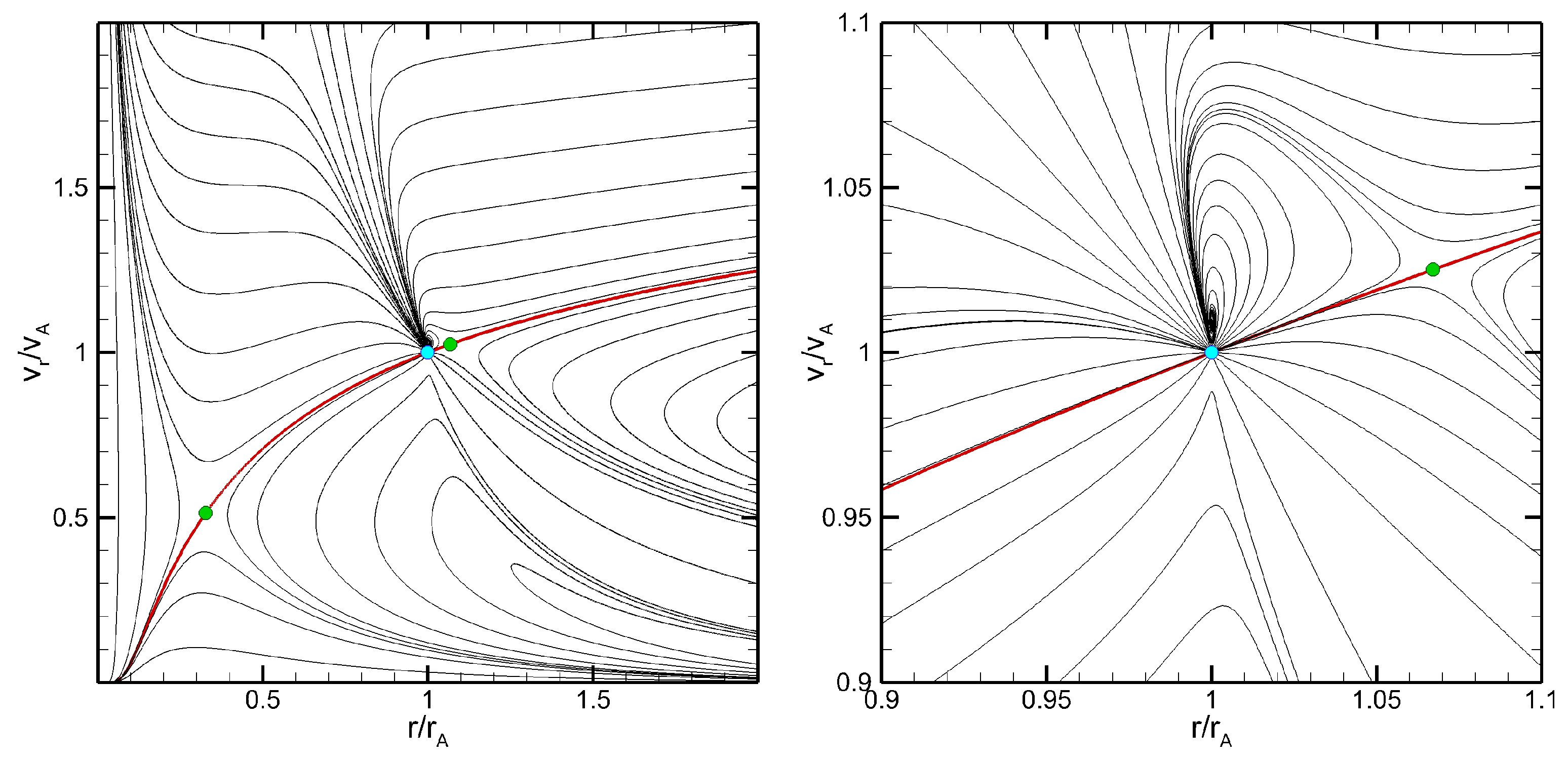
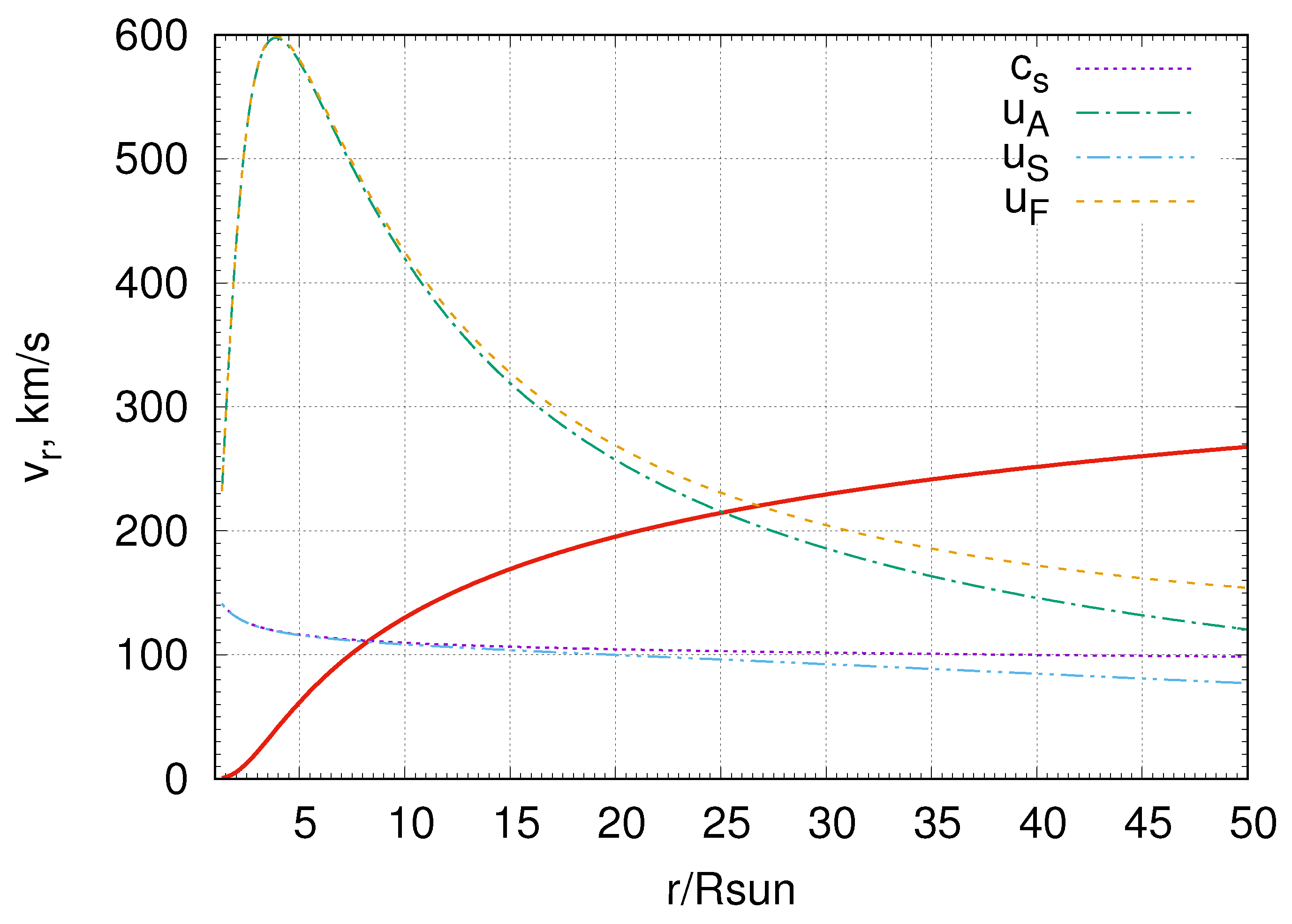
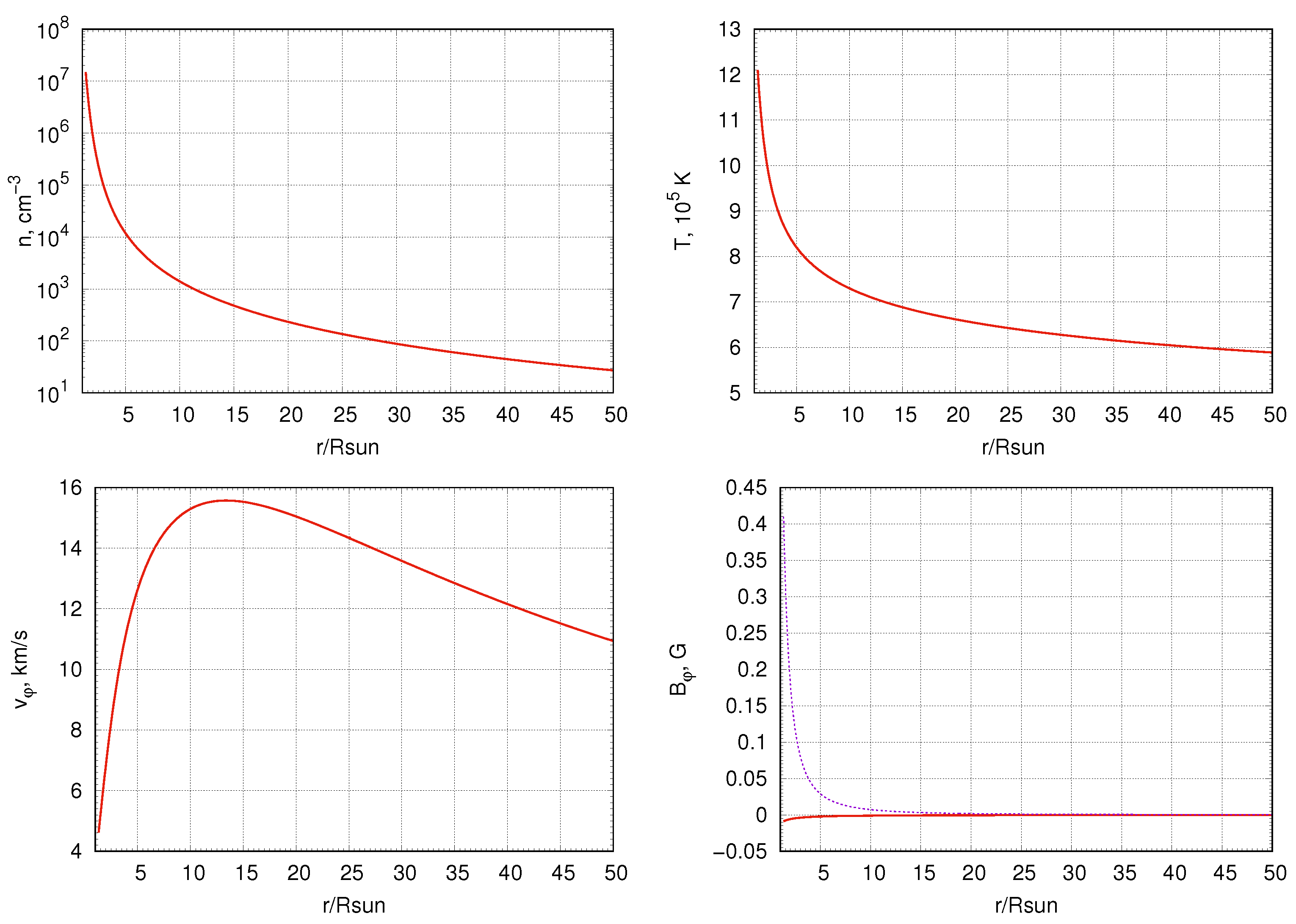
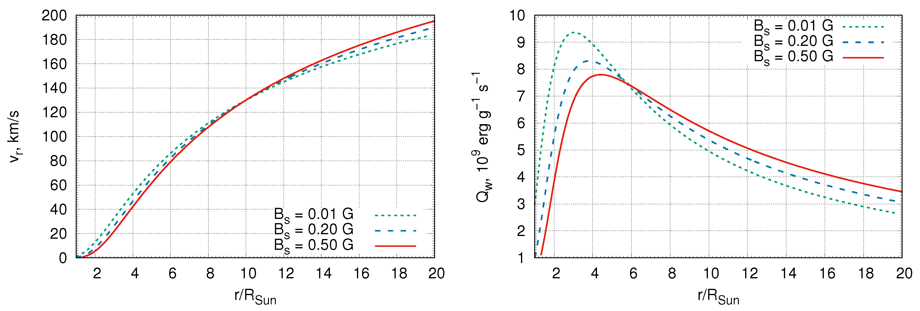
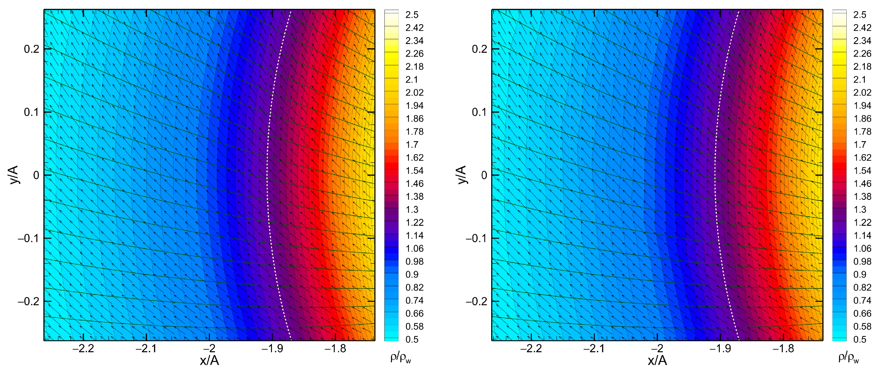
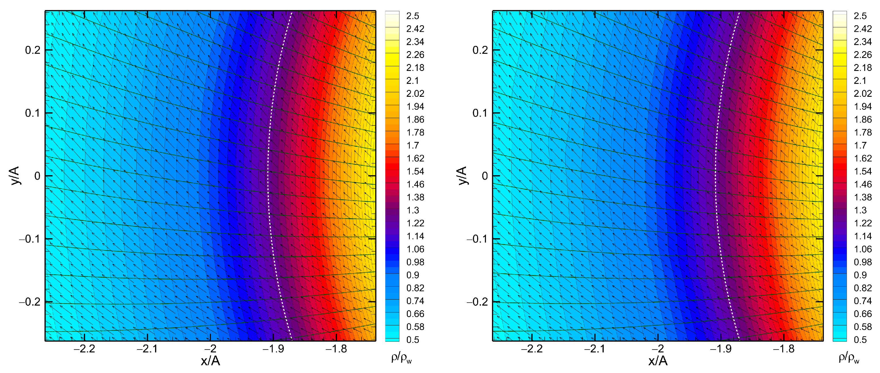
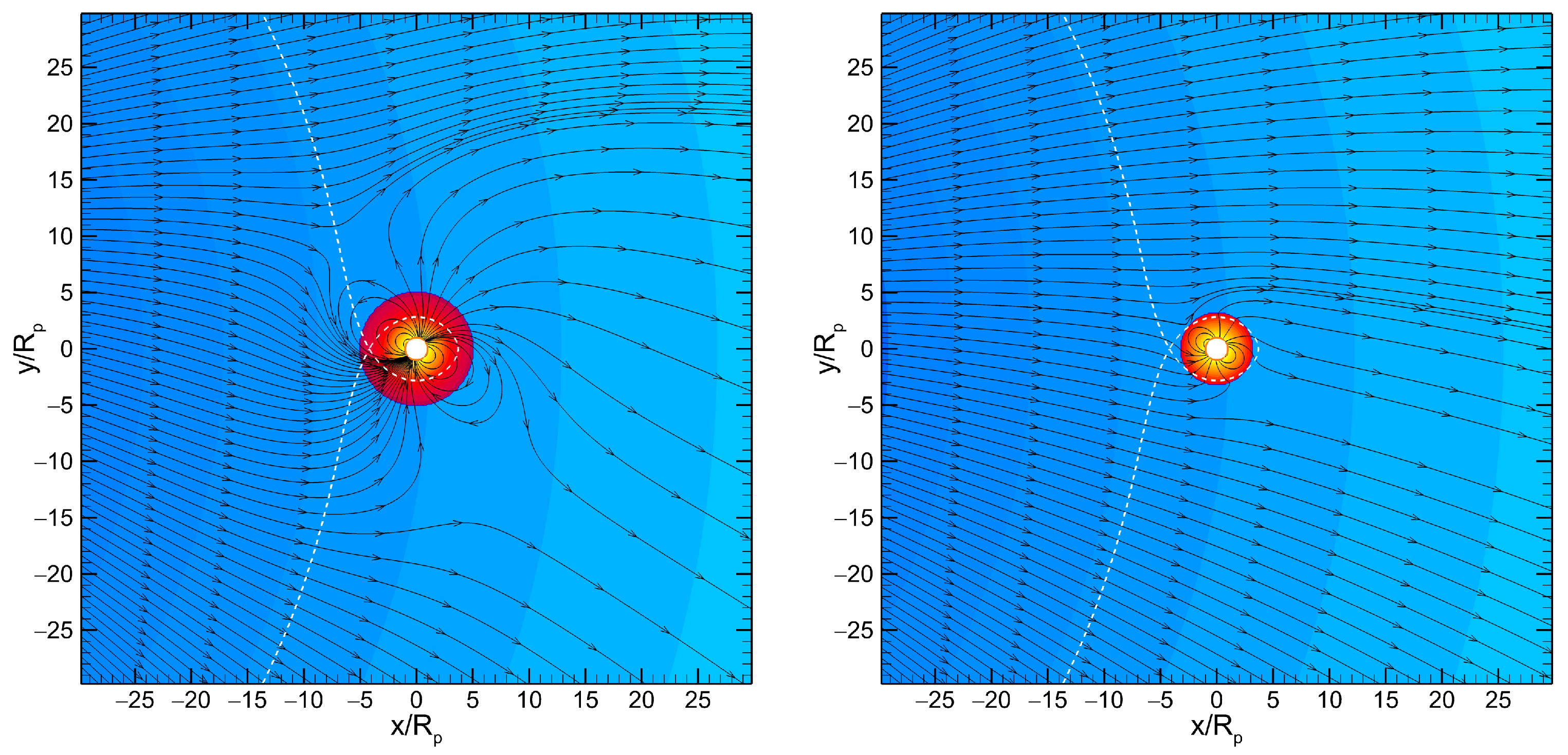
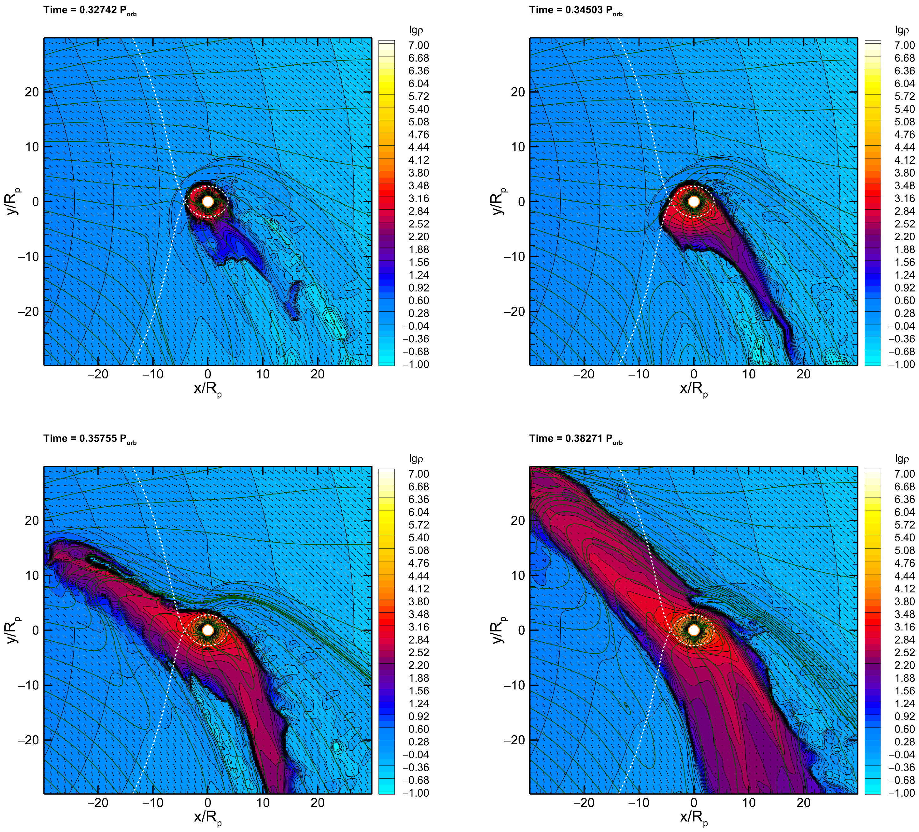
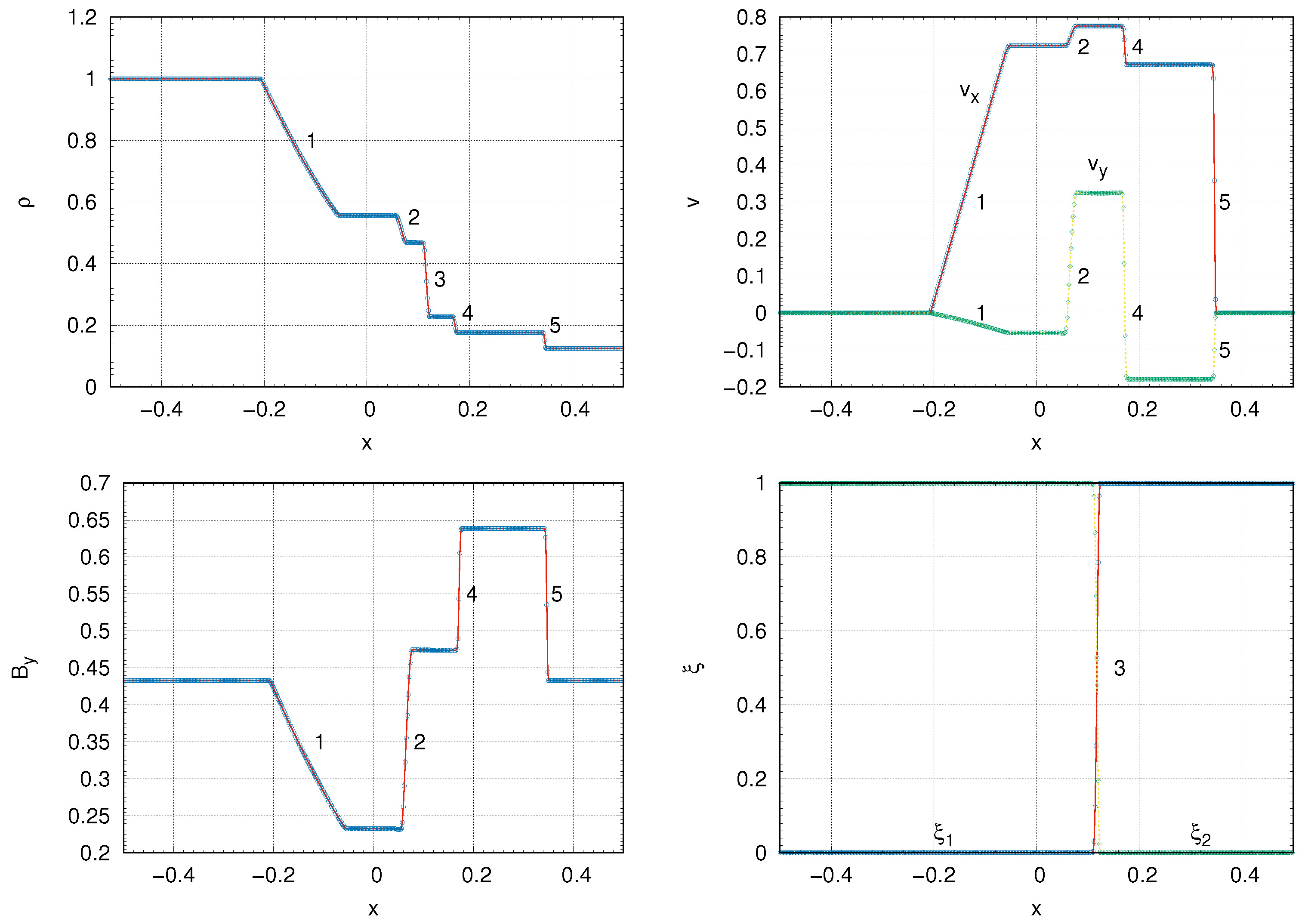
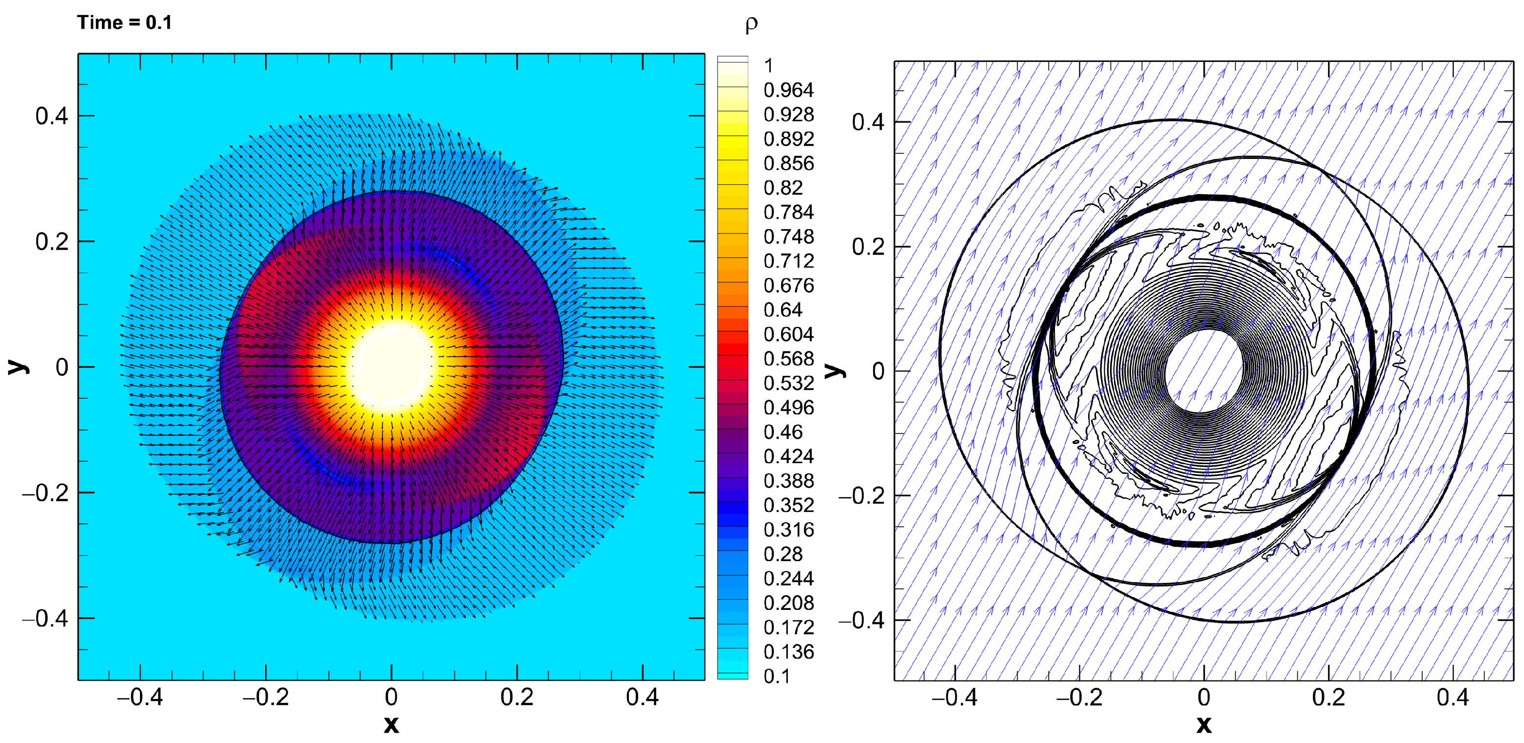
Table 1.
Parameters and characteristics of the models: is the temperature of the upper atmosphere, is the magnetic field of the star, and is the mass loss rate of the planet.
Table 1.
Parameters and characteristics of the models: is the temperature of the upper atmosphere, is the magnetic field of the star, and is the mass loss rate of the planet.
| Model | , K | , G | Flow Regime | Envelope Type | , 109 g/s |
|---|---|---|---|---|---|
| 1 | 5000 | 0.01 | Super-Alfvénic | Closed | 1 |
| 2 | 5500 | 0.01 | Super-Alfvénic | Quasi-closed | 1 |
| 3 | 6000 | 0.01 | Super-Alfvénic | Quasi-Opened | 4 |
| 4 | 6500 | 0.01 | Super-Alfvénic | Opened | 10 |
| 5 | 6500 | 0.2 | Trans-Alfvénic | Quasi-Opened | 9 |
| 6 | 6500 | 0.5 | Sub-Alfvénic | Quasi-Opened | 7 |
Publisher’s Note: MDPI stays neutral with regard to jurisdictional claims in published maps and institutional affiliations. |
© 2021 by the authors. Licensee MDPI, Basel, Switzerland. This article is an open access article distributed under the terms and conditions of the Creative Commons Attribution (CC BY) license (https://creativecommons.org/licenses/by/4.0/).
Share and Cite
MDPI and ACS Style
Zhilkin, A.; Bisikalo, D. Multi-Component MHD Model of Hot Jupiter Envelopes. Universe 2021, 7, 422. https://0-doi-org.brum.beds.ac.uk/10.3390/universe7110422
AMA Style
Zhilkin A, Bisikalo D. Multi-Component MHD Model of Hot Jupiter Envelopes. Universe. 2021; 7(11):422. https://0-doi-org.brum.beds.ac.uk/10.3390/universe7110422
Chicago/Turabian StyleZhilkin, Andrey, and Dmitri Bisikalo. 2021. "Multi-Component MHD Model of Hot Jupiter Envelopes" Universe 7, no. 11: 422. https://0-doi-org.brum.beds.ac.uk/10.3390/universe7110422
Note that from the first issue of 2016, this journal uses article numbers instead of page numbers. See further details here.