
Cosmological Perturbations via Quantum Corrections in M-Theory


1
Meijo University Senior High School, Shintomi-cho 1-3-16, Nakamura-ku, Nagoya 453-0031, Aichi, Japan
2
College of Science, Ibaraki University, Bunkyo 2-1-1, Mito 310-8512, Ibaraki, Japan
*
Author to whom correspondence should be addressed.
Universe 2021, 7(11), 425; https://0-doi-org.brum.beds.ac.uk/10.3390/universe7110425
Submission received: 6 October 2021
/
Revised: 29 October 2021
/
Accepted: 4 November 2021
/
Published: 7 November 2021
Abstract
:In the early universe, it is important to take into account the quantum effect of gravity to explain the feature of inflation. In this paper, we consider the M-theory effective action which consists of 11-dimensional supergravity and (Weyl) terms. The equations of motion are solved perturbatively, and the solution describes the inflation-like expansion in 4-dimensional spacetime. Equations of motion for tensor perturbations around this background are derived perturbatively. We also check that the equations of motion are obtained from the effective action up to the second order of the perturbations. Finally, we solve the equations of motion for the tensor perturbations perturbatively and obtain analytic expressions for them.
1. Introduction
Inflationary expansion of the early universe resolves problems of the hot Big Bang scenario, such as the horizon problem or flatness problem [1,2,3,4,5]. It also generates perturbations to the homogeneous background, which become initial conditions for the structure formation of the present universe. Recent observations of cosmological parameters restrict the quantities of these perturbations, and hence models of the inflation [6,7,8]. In order to realize the inflation via the 4-dimensional effective theory of gravity, it is usual to introduce an inflation field or some higher curvature terms1. The inflaton field causes the inflationary expansion while it slowly rolls down the potential [5,17,18,19,20]. The inflation via higher curvature term was first studied by Starobinsky [1], which is surprisingly consistent with the current observations.
Since the energy scale of the inflationary era will be near that of the grand unified theory, it is important to analyze this scenario by using ultraviolet completion of quantum gravity. Actually, there have been many attempts to explain the inflation from supergravity theory, which is a low-energy effective action of superstring theory. It is difficult, however, to obtain de Sitter (dS) vacua in the effective theory obtained by compactification of the supergravity theory, which is stated as a no-go theorem [21,22,23] or dS swampland conjecture [24,25,26]. Especially, the dS swampland conjecture says that low-energy effective theories which realize the inflation by the inflaton field cannot be consistent with quantum theory of gravity at Planck scale.
To evade the no-go theorem, we need to take into account corrections to the supergravity theory. One way is to introduce sources of branes in the superstring theory, and it was proposed in [27] that the de Sitter vacua can be constructed in the superstring theory with orientifold planes and flux compactification. Some recent consistency checks with the swampland conjecture are reported in [28]. Another way is to introduce higher curvature corrections in the superstring theory, and some earlier works in this direction can be found in [29,30,31,32,33].
In this paper, we pursue the possibility of the inflationary scenario in M-theory. The M-theory is defined as a strong coupling limit, or uplift to 11 dimensions, of type IIA superstring theory, and the low-energy limit is approximated by 11-dimensional supergravity. Since the type IIA superstring theory contains one-loop corrections, the uplift of these terms also gives corrections to the 11-dimensional supergravity. As for the metric, it gives products of four Weyl tensors, abbreviated as , so it is important to understand the effect of these terms in relation to the inflationary scenario in the M-theory. Actually, it is shown in [34,35] that if the spacetime is divided into four dimensions and seven internal spatial directions, we obtain a perturbative solution where the three spatial directions are expanding and the internal ones are shrinking. Scalar perturbations around the inflationary background are discussed in [36]. The purpose of this paper is to analyze tensor perturbations around the inflation-like background. Equations of motion for tensor perturbations around this background are derived perturbatively. In addition, we also check that the equations of motion are obtained from the effective action up to the second order of the perturbations. Finally, we solve the equations of motion for the tensor perturbations perturbatively and obtain analytic expressions for them.
The organization of this paper is as follows. In Section 2, we briefly review the background geometry of [34]. In Section 3, we consider the tensor perturbations around the background and obtain equations of motion perturbatively. The effective action for the tensor perturbations are also derived. In Section 4, we solve the equations of motion for the tensor perturbations perturbatively and obtain analytic solutions. Conclusions and discussion are given in Section 5. The scalar perturbations and their solutions are summarized in Appendix A. Some discussion on the power spectrum of the cosmological perturbations are given in Appendix B and Appendix C.
2. Effective Action and Inflationary Solution in M-Theory
Low-energy effective action of the superstring theory is obtained by analyzing scattering amplitudes [37,38] or conformal invariance of loop corrections on the string world-sheet [39,40]. The low-energy effective action of the M-theory is described by 11-dimensional supergravity, and its leading correction is obtained by uplifting the results of the type IIA superstring theory. The bosonic part of the effective action of the M-theory is given by [41,42]
where are local Lorentz indices and is a Weyl tensor2. The 11-dimensional gravitational constant and a coefficient are dimensionful parameters and expressed in terms of the 11-dimensional Planck length as
Note that the above action can be derived directly in 11 dimensions by imposing local supersymmetry [43,44,45,46,47,48,49]. The Z terms in the action (1) are related to a topological term via local supersymmetry and the numerical values in this action are protected against higher perturbations. Of course, there exist higher derivative terms of for , but those contributions are unknown so far. Some thoughts on the possible terms of can be found in [36].
In this paper, we solve the equations of motion perturbatively up to the linear order of . By varying the effective action (1), we obtain following equations of motion [50]3.
Here, is a covariant derivative for local Lorentz index, and tensors and are defined as
where , and .
Let us consider the solution of effective action (1) in the early universe. We assume that the 10-dimensional space directions are divided into a 3-dimensional flat homogeneous space and a 7-dimensional internal space compactified on the 7-dimensional flat torus. Then, the ansatz of the metric is expressed as
where and . and are scale factors for the 3-dimensional space and the 7-dimensional internal one, respectively. By inserting the above ansatz into Equation (4), we obtain differential equations for and . Here, the dot represents the time derivative. The solution up to linear order of is given by [34]
with
Here, is an integral constant and is defined by
Notice that is the dimensionless parameter and takes the range of . By integrating Equation (8), the scale factors and are written as
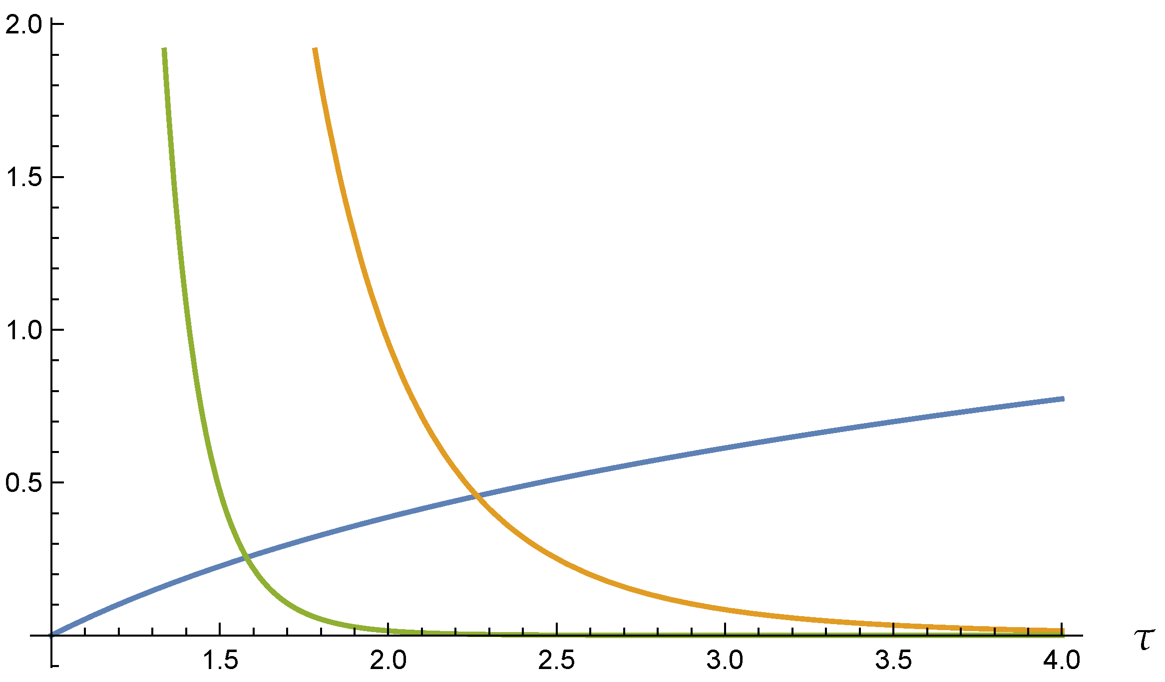
respectively. Here, and are integral constants and correspond to scale factors around the end of the inflation or the deflation, respectively. Since the string theory suppresses the divergence in the UV region, we expect that the scale factor and become convergent functions in the region . This means that coefficients of the higher-order terms will become the same order. In Figure 1, we show plots of , and for and , respectively. From this, we see that higher-order corrections are suppressed in the region , and the inflationary expansion or deflation is realized by each term in Equation (11).
The motivation for the inflation is to resolve the horizon problem. This requires that the particle horizon during the inflationary era is almost equal to that after the radiation-dominated era. The particle horizon during the inflationary era is given by
On the other hand, if we approximate the scale factor as after , the particle horizon during this era is evaluated as
where is the value at current time . We also obtain .
Now we define the e-folding number as . This means that . By equating Equation (12) with Equation (13), we obtain
This gives a relation between and , and we obtain for , for example.
We also obtain for .
3. Tensor Perturbations in M-Theory
3.1. Equations of Motion for the Tensor Perturbations
In this section, we investigate the tensor perturbations around the background geometry (7) up to the linear order of . Since the action (1) contains complicated terms, we employ a Mathematica code to obtain the results here, even though these expressions are analytic. We deal with equations of motion for perturbations order by order, in the spirit of [51]. We also consult the calculations of cosmological perturbations in the modified gravity [52,53].
The tensor perturbations around the background metric are chosen as follows:
In addition, can be divided into two polarization modes, and . In the vielbein formalism, it is expressed as
up to the linear order of the perturbation. Linearized equations of motion for the metric perturbations are obtained by varying Equation (4). The result is given as follows:
In this paper, we will solve the above equations of motion in the momentum space for the tensor perturbations. are expanded as
where is a momentum in the 3 spatial directions, and is a discretized momentum on the internal 7-dimensional torus. The internal momentum appears in the equations of motion with a factor of , so these terms decouple from the equations of motion as b becomes quite small during the inflation [36]. Hence, we neglect the contributions of internal momentum in this paper.
By inserting the expression (16) into the equations of motion (17), we obtain following differential equation for :
where are functions of H and G. The explicit forms of are derived by employing Mathematica codes, which are reported in [54], and the results are written as
and
Since we solve the equations of motion up to the linear order of , we expand H, G and as
Notice that and are the leading parts of the background (8), and satisfy and . We substitute these into Equation (19) and expand it up to the linear order of . Finally, with the aid of Mathematica code [54], we obtain the explicit forms of the equations of motion. The equation of motion for is written as
In addition, the equation of motion for is given by
3.2. Effective Action for the Tensor Perturbations
In this subsection, we show an effective action for the tensor perturbations up to the second order of . This is important to fix the normalization of the tensor perturbations as well as to perform a consistency check of the equations of motion.
The effective action for is obtained by substituting the perturbation (16) into the action (1). The results are derived by using the Mathematica code [54], and the effective action for is obtained as
In addition, explicit forms of are given by
and
While not shown explicitly, it is also possible to write down the effective action for , which is slightly different from the above expression. We remark, however, that the effective action for is the same as that of after substituting the background metric.
By substituting Equation (25) into the action (28), we obtain the effective action for the tensor perturbation up to the second order of and . The result is
Here, and .
It is easy to see that the equation of motion (26) is obtained from the variation of ,
Here, we used the relation of the background . Note also the relations of , and . By using these relations, it is possible to evaluate the variation of the effective action with respect to as
4. Solution for the Tensor Perturbations
Let us analytically solve Equations (26) and (27) in this section. In order to solve these equations, we introduce a new time coordinate instead of t, which is defined by . This means that behaves like a conformal time after the inflationary expansion. Now, is expressed in terms of as
and and a Hubble parameter with respect to are given by
Here, the prime represent . Then, by defining and multiplying to Equation (26), we obtain
In addition, the above differential equation for can be solved as
Here, and are Bessel functions of the first and second kind, respectively. and are integral constants which have the dimension of mass and depend on k. In order to fix the ratio of , we demand that behaves like as goes to infinity. This means that the tensor perturbation is approximated by the free field as goes to infinity. Since and as , we choose and is given by
is the Hankel function of the second kind. is proportional to and the coefficient is determined by the normalization of the action (32). From this, is expressed as
If we take , approaches to .
Next, we investigate the equation of motion (27) for . By multiplying to Equation (27) and using , we obtain
In order to solve the above equation, we redefine as . Then, a differential equation for is expressed as
In the second line, we substituted Equations (36) and (38). A particular solution for the above equation is given by
Here, the explicit forms of and are given by
and
Here, the function is the generalized Meijer G-function, and the function is the generalized hypergeometric function. The ratio of should be fixed by as explained before. Thus, we have solved Equation (41) as
Here, we used .
In conclusion, we derived analytic form of the tensor perturbations which are given by Equations (40) and (46). If we know the effective action of the M-theory beyond the linear order of , we could derive the solution up to the same order by using the method developed in this paper. Some discussions on the power spectrum of the perturbations are given in Appendix B.
5. Conclusions and Discussion
In this paper, we examined the inflationary solution via higher derivative corrections in the M-theory and examined tensor perturbations around such a background. As a result, we have obtained the solutions of tensor perturbations analytically up to the linear order of . Although our calculations are limited up to the linear order of , our method developed in this paper is applied to higher-order effective action once its form is revealed.
The effective action of the M-theory contains (Weyl) terms. If we assume that the 10-dimensional space is divided into a 3-dimensional homogeneous space and a 7-dimensional internal one, it is possible to solve the equations of motion perturbatively with respect to and obtain a inflationary solution due to the presence of (Weyl) terms. The tensor perturbations are analyzed around this inflationary background. These are expanded up to the linear order of such as , and the equation of motion for is written by Equation (26) and that for is given by Equation (27). On the other hand, the effective action for the tensor perturbation for the cross mode is evaluated up to the linear order of . In addition, the effective action with respect to and is given by Equation (32). We could derive the same equations of motion from this action, and this gives a self-consistency check of our calculations, which are mainly done by using Mathematica codes. Although we omitted the calculations, the effective action for the plus mode is the same as that of the cross mode once we insert the background metric.
The equations of motion for are solved perturbatively. The solution of is given by the linear combinations of Bessel functions. Then, we put the solution of into the equation of motion for . The analytic form of is given by Equation (46). In this way, we developed a method to calculate tensor perturbations by using Mathematica codes. If we know the effective action of the M-theory beyond the linear order of , we could derive the solution up to the same order by using the method developed in this paper [55].
Since we know the analytic solution, at least perturbatively, it is straightforward to evaluate the power spectrum of the tensor perturbations. However, the vacuum of our inflationary solution is highly interacting, it is different from usual Bunch–Davies vacuum. So, in order to evaluate the power spectrum, we need to put an assumption on the amplitude of the power spectrum. Some discussions on the evaluation of the power spectrum are given in Appendix B.
As a future work, it is interesting to apply the method developed here to more a complicated internal geometry, such as the manifold [56]. It is also interesting to apply the analyses of this paper to the heterotic superstring theory with nontrivial internal space, which contains corrections [57], and reveal several problems in string cosmology [58]. Unification of the inflationary expansion and late time acceleration in modified gravity, such as gravity or mimetic gravity, is an interesting direction to be explored [59,60,61,62].
Author Contributions
Conceptualization, Y.H.; methodology, K.H. and Y.H; software, K.H. and Y.H.; validation, K.H. and Y.H.; formal analysis, K.H. and Y.H.; investigation, K.H. and Y.H.; resources, K.H. and Y.H.; data curation, K.H. and Y.H.; writing—original draft preparation, Y.H.; writing—review and editing, K.H. and Y.H.; visualization, K.H. and Y.H.; supervision, Y.H.; project administration, Y.H.; funding acquisition, Y.H. All authors have read and agreed to the published version of the manuscript.
Funding
This work was partially supported by Japan Society for the Promotion of Science, Grant-in-Aid for Scientific Research (C) Grant Number JP17K05405.
Acknowledgments
The authors would like to thank Takanori Fujiwara and Makoto Sakaguchi. This work was partially supported by Japan Society for the Promotion of Science, Grant-in-Aid for Scientific Research (C) Grant Number JP17K05405.
Conflicts of Interest
The authors declare no conflict of interest.
Appendix A. The Scalar Perturbations
In this appendix, we briefly summarize the results of scalar perturbations obtained in [36]. The metric for the scalar perturbations is written as
By inserting the above into Equation (17), we obtain four independent equations with respect to , and . By using two equations out of four, it is possible to solve and up to the linear order of , and one equation becomes redundant. Then, we obtain a differential equation for up to the linear order of .
As in the case of the tensor perturbations, in order to solve Equation (A2), we use the variable which is defined in Equation (35). By multiplying to Equation (A2), we obtain
Let us solve the above equation perturbatively. First, by setting , a part of becomes
This is the same as Equation (37). Then, , and are solved as follows:
In the above, we set as in the tensor perturbations. is proportional to and the coefficient is determined by the normalization of the action in [36]. In the limit of , approaches to .
Next, let us solve a part of the differential Equation (A3) which linearly depends on . By setting and using the solution (A5), the equation which linearly depends on becomes
A particular solution of the above is obtained by using Mathematica code [36]. The solutions of , and are expressed as follows.
Appendix B. Numerical Analyses for Scalar and Tensor Perturbations
In this appendix, we examine spectral indices of the scalar and tensor perturbations. First of all, we change the definition of by rescaling. Without loss of generality, it is possible to rescale like
In addition, after this prescription, we shift the integral constants as
Then, , , , and are invariant, and , , and behave as
Note that the range of becomes . Thus, the parameter disappears from the background and is absorbed into the lower bound of , which is determined by requiring that the e-folding number is within the range of . Below we use Equation (A10) as the background and the range of is given by . The explicit value of is irrelevant in this paper but should be determined by the e-folding number4. From Equation (35), is also bounded as
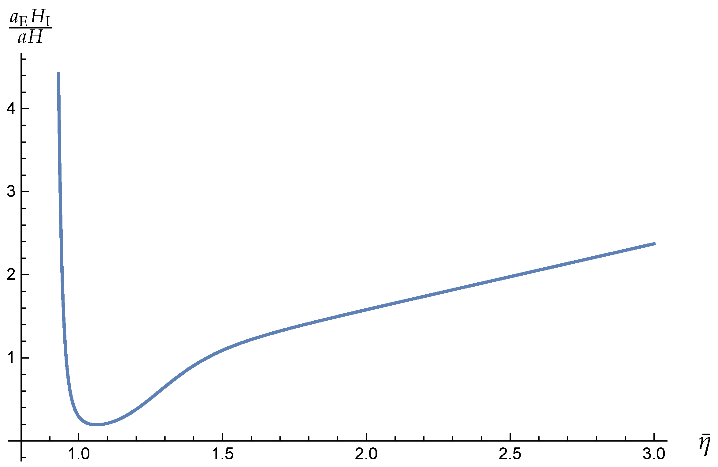
Here, we introduced the dimensionless parameter , and corresponds to . Below, we assume that the expansions in Equation (A10) are convergent around and coefficients of higher-order terms in Equation (A10) are small and negligible around 5. A plot of the comoving Hubble radius as a function of is shown in Figure A1. From this figure, we see that the inflation ends around .
Figure A1.
Plot of the comoving Hubble radius as a function of .

First, let us evaluate the power spectrum of the tensor perturbation. In Section 4, we normalized the tensor perturbation around the vacuum in the future infinity, . In addition, the quantization of the tensor perturbation becomes
is given by Equation (39) and is written by Equation (43). However, the power spectrum should be evaluated by using the vacuum in the past infinity, so we need the Fourier component, which we denote , solved in the past infinity. Although the quantization of the tensor perturbation around the vacuum in the past infinity is difficult due to the complicated interaction, and are related by the Bogoliubov transformation as
with some unknown functions of and . Then, an ingredient of the power spectrum is evaluated as
where , and are arguments of , and , respectively. The second term in the big parentheses is less than 1. In the above expression, the dependence appears through and . So, if is almost time independent, the ingredient of the power spectrum is approximated as
with some unknown function . We show a plot of for small k and justify the above approximation in Appendix C.
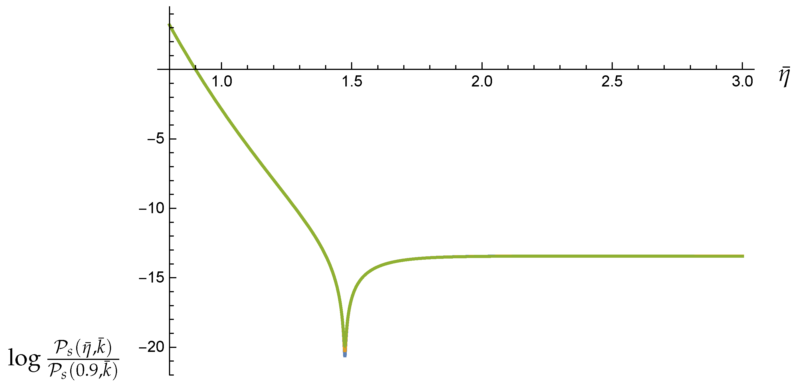
From the above argument and using Equations (40) and (46), the power spectrum of the tensor perturbations is approximated as
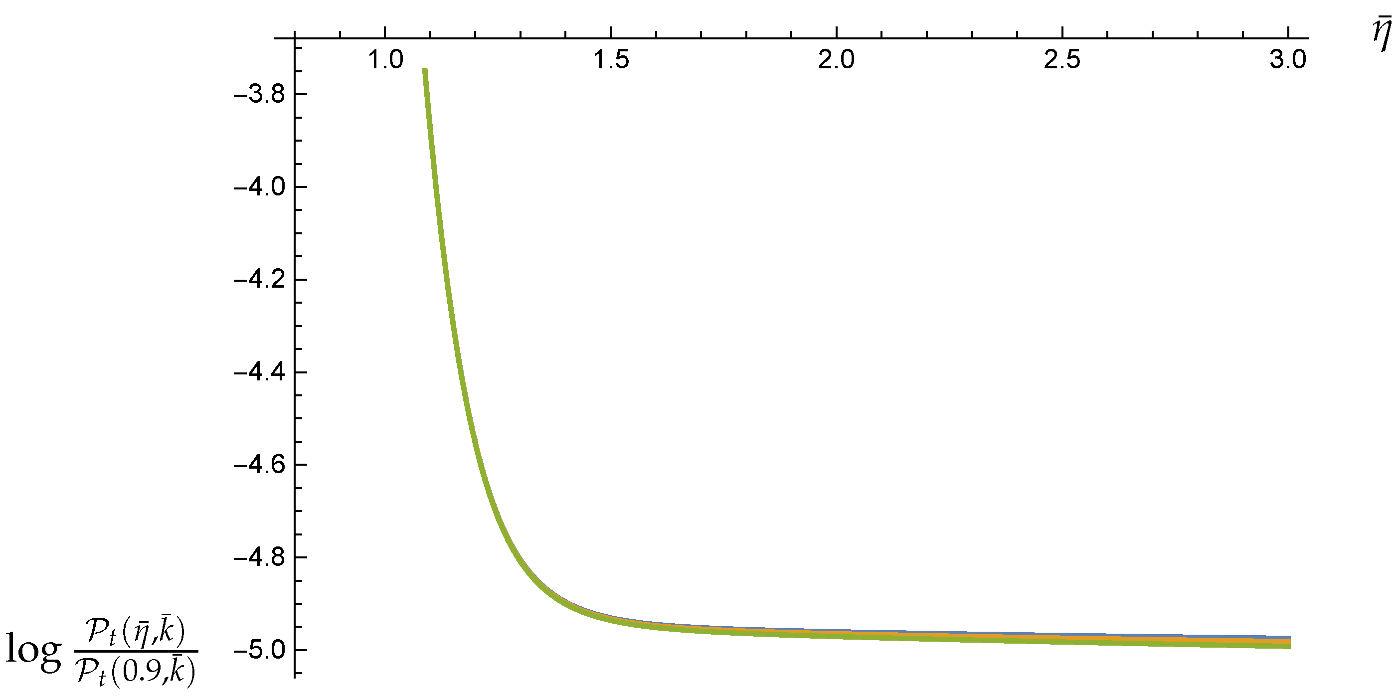
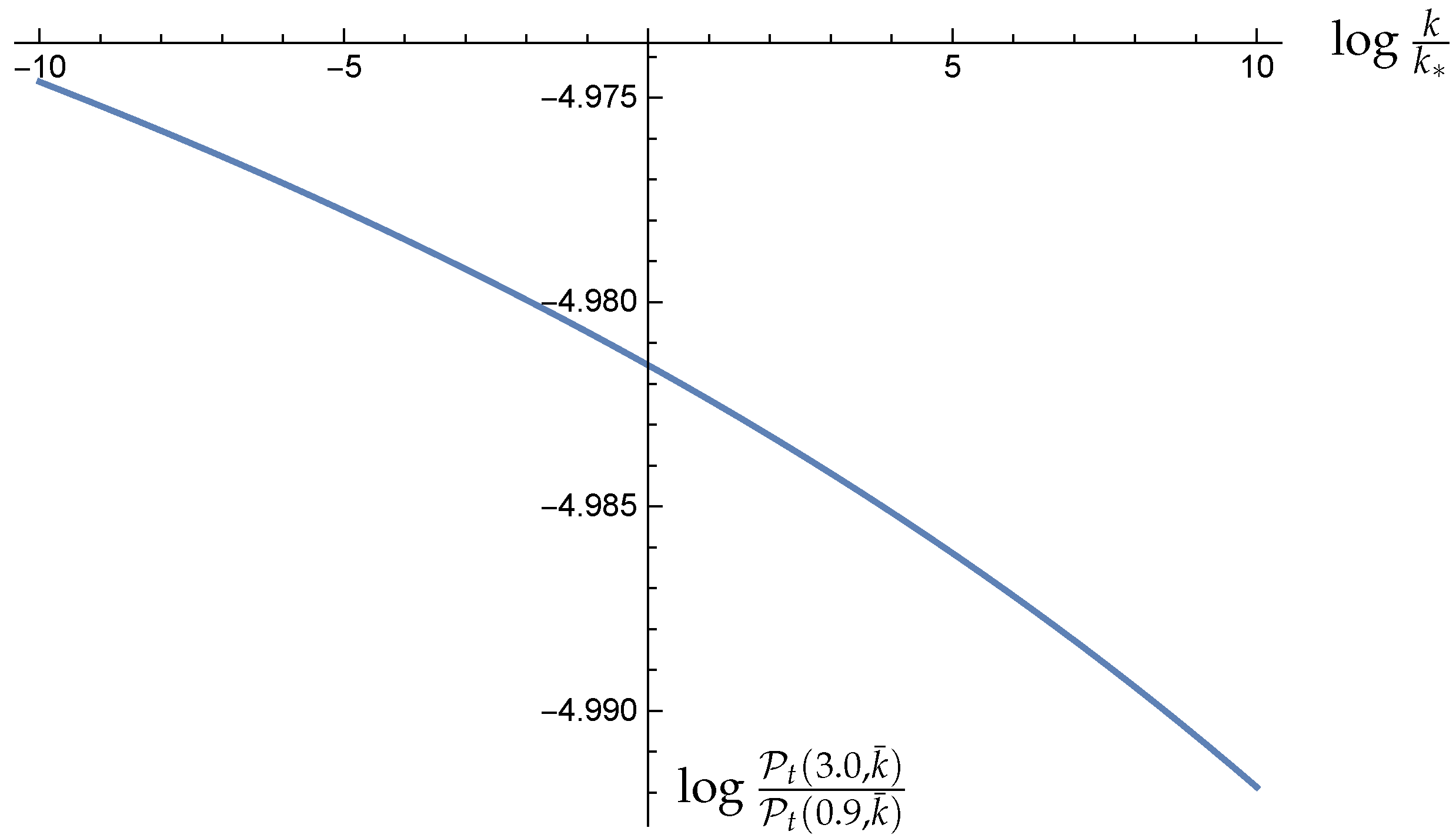
where and is a dimensionless momentum6. Since cannot be determined, we normalize the power spectrum as . Plots of these functions with and are shown in Figure A2. Naively, the horizon exit occurs at , but the corrections should modify this relation. Thus, we define the spectral index by evaluating the power spectrum at , where the scale factor behaves like a radiation-dominated era. A function of is plotted in Figure A3. If we fit the curve, we obtain
From this expression, we see that the tensor spectral index becomes and its runnings are quite small. Thus, if the power spectrum is independent of k at the beginning of the inflation, it is almost scale-independent after the inflation. Note that if we evaluate at , it becomes closer to zero.
Figure A2.
Plots of with (blue), (yellow) and (green).

Figure A3.
Plots of as a function of .

Next, by applying the similar argument for Equation (A15), it is possible to relate the scalar perturbation defined in the past infinity to in the future infinity. and are given by Equations (A5) and (A7), respectively.
Then, by using Equations (A5) and (A7), the power spectrum of the scalar perturbations is expressed as
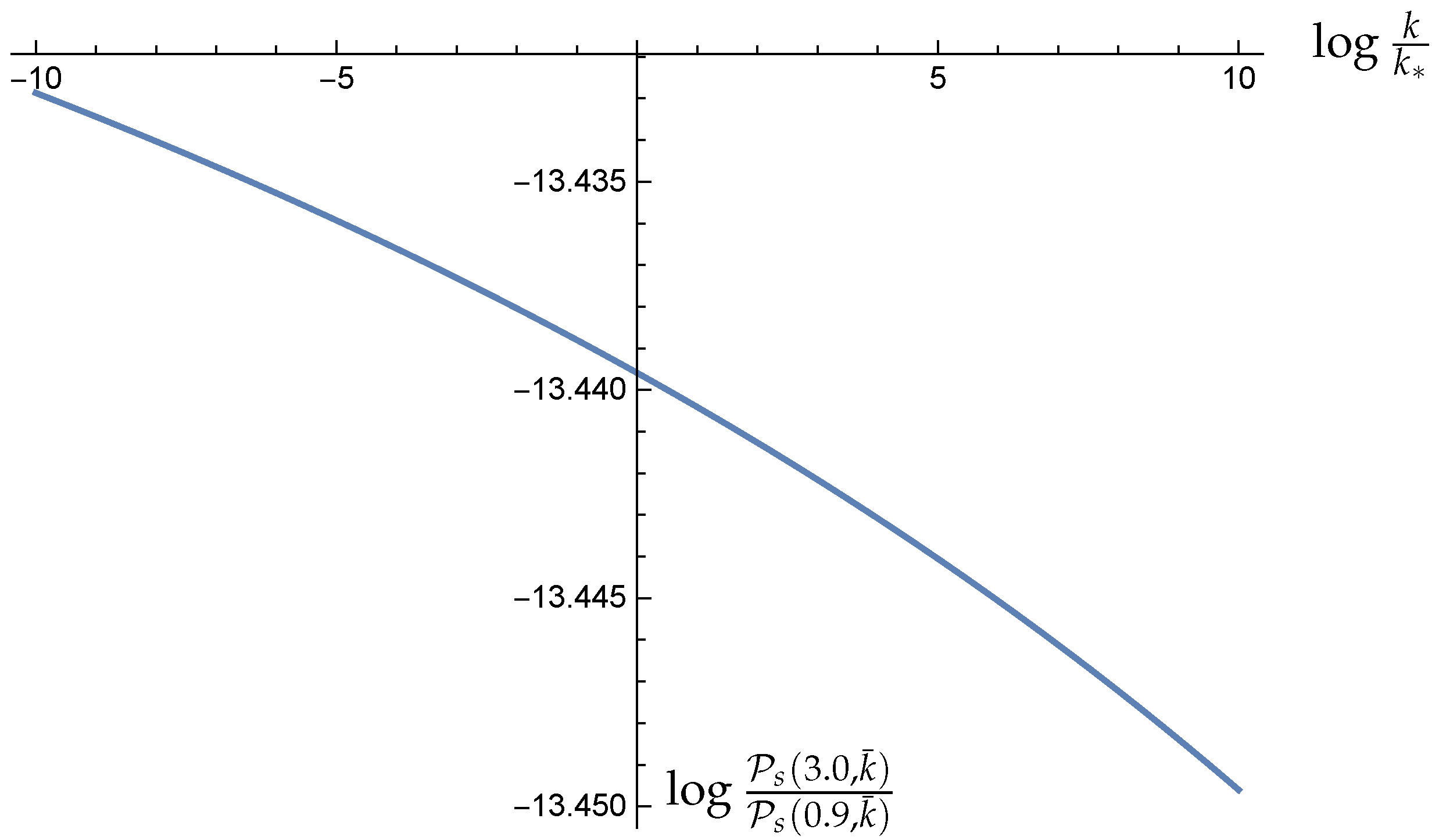
where . Since the dimensional parameter cannot be determined, we normalize the power spectrum as . Plots of these functions with and are shown in Figure A4. In addition, a function of is plotted in Figure A5. If we fit the data, we obtain
From this expression, we see that the spectral index becomes and its runnings are quite small. Again, if the power spectrum is independent of k at the beginning of the inflation, it is almost scale-independent after the inflation. Note that if we evaluate at , it becomes closer to one.
Figure A4.
Plots of with (blue), (yellow) and (green).

Figure A5.
Plots of as a function of .

The tensor-to-scalar ratio r is obtained by the power spectra of scalar and tensor perturbations. If we define r at (), we obtain
Here, we used and . Since , we need that the power spectrum of the tensor perturbation is much smaller than that of the scalar perturbation at the beginning of the inflation [8]. The mechanism of this process is not clear so far, and the knowledge of the behaviors of perturbations around should be quite important. In this section, we assumed that power spectra and are scale-invariant, but it will be interesting if we can restrict these values from the observation.
Appendix C. Plots of θu and θU
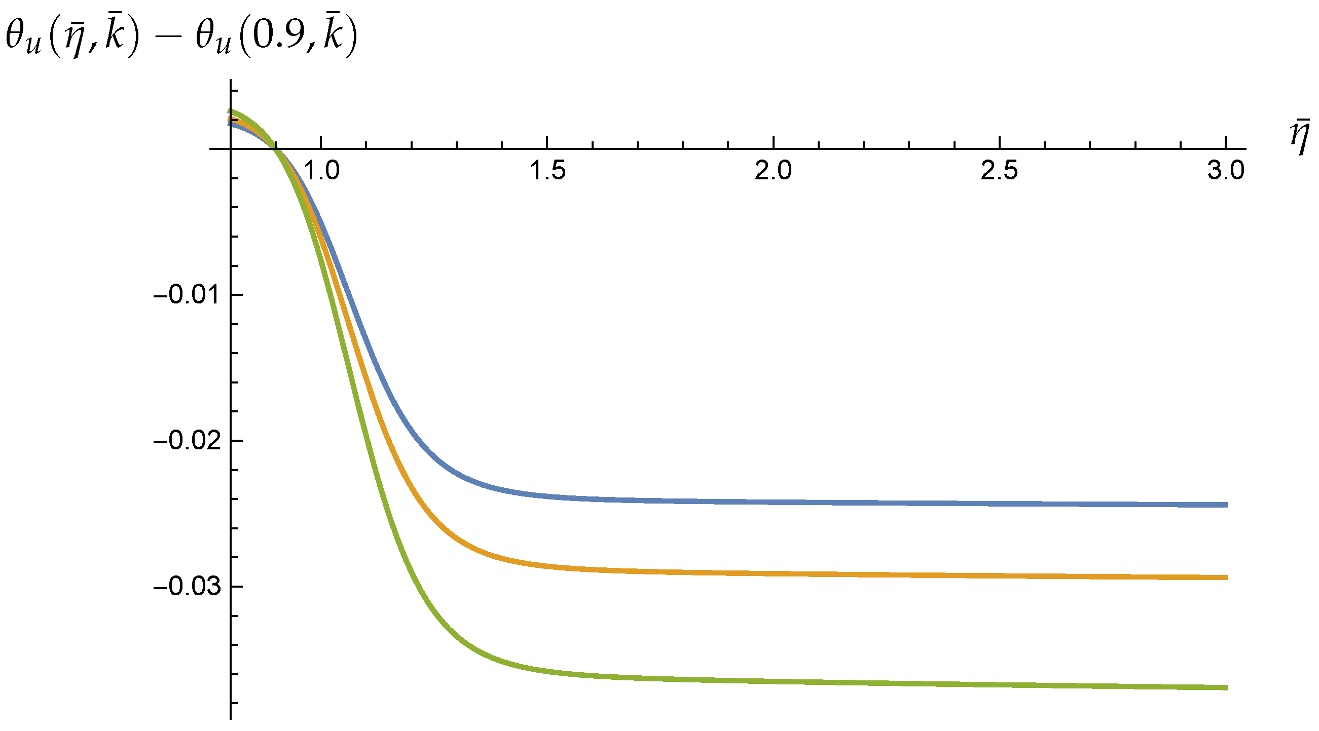
is the argument of . and are given by Equations (39) and (43), respectively. We also prescribe the rescaling of (A8) and (A9). Then, the plots of with and are shown in Figure A6. From these plots, we see that is almost time-independent for .
Figure A6.
Plots of [rad] with (blue), (yellow) and (green).

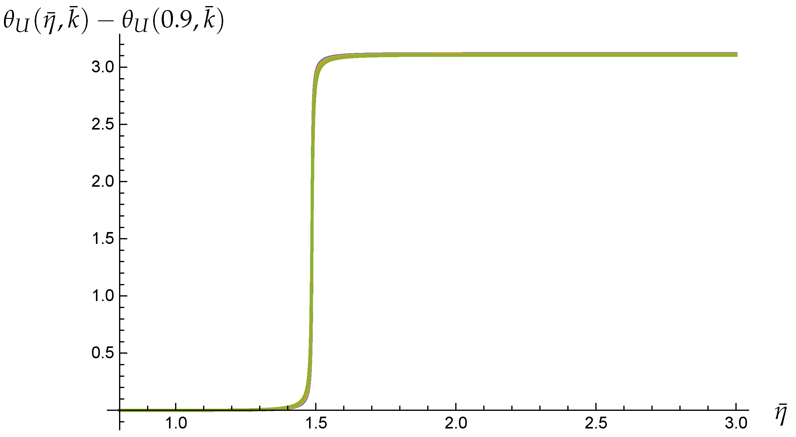
is the argument of . and are given by Equations (A5) and (A7), respectively. We also prescribe the rescaling of (A8) and (A9). Then, the plots of with and are shown in Figure A7. From these plots, we see that, except around , is almost time-independent for .
Figure A7.
Plots of [rad] with (blue), (yellow) and (green).

| 1 | |
| 2 | It is possible to make the Riemann tensor to a Weyl tensor by using field redefinition ambiguity. A more general case is discussed in [35]. |
| 3 | The action contains linear term on 3-form field A which is proportional to
|
| 4 | For example, corresponds to () [36]. Higher derivative terms which are not considered in this paper will also affect the explicit value of . |
| 5 | Some thoughts on this point are given in the appendix in [36]. |
| 6 | A sum of physical degrees of freedom are included in . As discussed in the Section 2, we choose and define a pivot scale as . |
References
- Starobinsky, A.A. A New Type of Isotropic Cosmological Models Without Singularity. Phys. Lett. 1980, 91B, 99. [Google Scholar] [CrossRef]
- Guth, A.H. The Inflationary Universe: A Possible Solution to the Horizon and Flatness Problems. Phys. Rev. D 1981, 23, 347. [Google Scholar] [CrossRef] [Green Version]
- Kazanas, D. Dynamics of the Universe and Spontaneous Symmetry Breaking. Astrophys. J. 1980, 241, L59. [Google Scholar] [CrossRef]
- Sato, K. First Order Phase Transition of a Vacuum and Expansion of the Universe. Mon. Not. Roy. Astron. Soc. 1981, 195, 467. [Google Scholar] [CrossRef]
- Linde, A.D. Chaotic Inflation. Phys. Lett. 1983, 129B, 177. [Google Scholar] [CrossRef]
- Ade, P.A.; Aghanim, N.; Ahmed, Z.; Aikin, R.W.; Alexander, K.D.; Arnaud, M.; Aumont, J.; Baccigalupi, C.B.; Ay, A.J.; Barkats, D.; et al. Joint Analysis of BICEP2/Keck Array and Planck Data. Phys. Rev. Lett. 2015, 114, 101301. [Google Scholar] [CrossRef] [Green Version]
- Ade, P.A.R.; Ahmed, Z.; Aikin, R.W.; Alexander, K.D.; Barkats, D.; Benton, S.J.; Bischoff, C.A.; Bock, J.J.; Bowens-Rubin, R.; Brevik, J.A.; et al. Improved Constraints on Cosmology and Foregrounds from BICEP2 and Keck Array Cosmic Microwave Background Data with Inclusion of 95 GHz Band. Phys. Rev. Lett. 2016, 116, 031302. [Google Scholar] [CrossRef] [PubMed]
- Akrami, Y.; Arroja, F.; Ashdown, M.; Aumont, J.; Baccigalupi, C.; Ballardini, M.; Banday, A.J.; Barreiro, R.B.; Bartolo, N.; Basak, S.; et al. Planck 2018 results. X. Constraints on inflation. Astron. Astrophys. 2020, 641, A10. [Google Scholar]
- Kolb, E.W.; Turner, M.S. The Early Universe. Front. Phys. 1990, 69, 1. [Google Scholar]
- Liddle, A.R.; Lyth, D.H. Cosmological Inflation and Large Scale Structure; Cambridge University Press: Cambridge, UK, 2000. [Google Scholar]
- Dodelson, S. Modern Cosmology; Academic Press: Amsterdam, The Netherlands, 2003. [Google Scholar]
- Weinberg, S. Cosmology; Oxford University Press: Oxford, UK, 2008. [Google Scholar]
- Linde, A. Inflationary Cosmology after Planck 2013. arXiv 2013, arXiv:1402.0526. [Google Scholar]
- Baumann, D.; McAllister, L. Inflation and String Theory; Cambridge University Press: Cambridge, UK, 2015. [Google Scholar]
- Felice, A.D.; Tsujikawa, S. f(R) theories. Living Rev. Rel. 2010, 13, 3. [Google Scholar]
- Nojiri, S.; Odintsov, S.D.; Oikonomou, V.K. Modified Gravity Theories on a Nutshell: Inflation, Bounce and Late-time Evolution. Phys. Rept. 2017, 692, 1. [Google Scholar] [CrossRef] [Green Version]
- Freese, K.; Frieman, J.A.; Olinto, A.V. Natural inflation with pseudo - Nambu-Goldstone bosons. Phys. Rev. Lett. 1990, 65, 3233. [Google Scholar] [CrossRef] [PubMed]
- Linde, A.D. Hybrid inflation. Phys. Rev. D 1994, 49, 748. [Google Scholar] [CrossRef] [PubMed]
- Boubekeur, L.; Lyth, D.H. Hilltop inflation. J. Cosmol. Astropart. Phys. 2005, 0507, 010. [Google Scholar] [CrossRef] [Green Version]
- Bezrukov, F.L.; Shaposhnikov, M. The Standard Model Higgs boson as the inflaton. Phys. Lett. B 2008, 659, 703. [Google Scholar] [CrossRef] [Green Version]
- Gibbons, G.W. Aspects Of Supergravity Theories. In Supersymmetry, Supergravity, and Related Topics; World Scientific Publishing: Singapore, 1985. [Google Scholar]
- Maldacena, J.M.; Nunez, C. Supergravity description of field theories on curved manifolds and a no go theorem. Int. J. Mod. Phys. A 2001, 16, 822. [Google Scholar] [CrossRef]
- Gibbons, G.W. Thoughts on tachyon cosmology. Class. Quant. Grav. 2003, 20, S321. [Google Scholar] [CrossRef]
- Obied, G.; Ooguri, H.; Spodyneiko, L.; Vafa, C. De Sitter Space and the Swampland. arXiv 2018, arXiv:1806.08362. [Google Scholar]
- Garg, S.K.; Krishnan, C. Bounds on Slow Roll and the de Sitter Swampland. J. High Energy Phys. 2019, 11, 075. [Google Scholar] [CrossRef] [Green Version]
- Ooguri, H.; Palti, E.; Shiu, G.; Vafa, C. Distance and de Sitter Conjectures on the Swampland. Phys. Lett. B 2019, 788, 180–184. [Google Scholar] [CrossRef]
- Kachru, S.; Kallosh, R.; Linde, A.D.; Trivedi, S.P. De Sitter vacua in string theory. Phys. Rev. D 2003, 68, 046005. [Google Scholar] [CrossRef] [Green Version]
- Blumenhagen, R.; Brinkmann, M.; Klaewer, D.; Makridou, A.; Schlechter, L. KKLT and the Swampland Conjectures. arXiv 2020, arXiv:2004.09285. [Google Scholar]
- Ishihara, H. Cosmological Solutions of the Extended Einstein Gravity With the Gauss-Bonnet Term. Phys. Lett. B 1986, 179, 217. [Google Scholar] [CrossRef]
- Ohta, N. Accelerating cosmologies and inflation from M/superstring theories. Int. J. Mod. Phys. A 2005, 20, 1. [Google Scholar] [CrossRef] [Green Version]
- Maeda, K.I.; Ohta, N. Inflation from M-theory with fourth-order corrections and large extra dimensions. Phys. Lett. B 2004, 597, 400. [Google Scholar] [CrossRef] [Green Version]
- Maeda, K.i.; Ohta, N. Inflation from superstring /M theory compactification with higher order corrections. I. Phys. Rev. D 2005, 71, 063520. [Google Scholar] [CrossRef] [Green Version]
- Akune, K.; Maeda, K.i.; Ohta, N. Inflation from superstring/M-theory compactification with higher order corrections. II. Case of quartic Weyl terms. Phys. Rev. D 2006, 73, 103506. [Google Scholar] [CrossRef] [Green Version]
- Hiraga, K.; Hyakutake, Y. Inflationary Cosmology via Quantum Corrections in M-theory. Prog. Theor. Exp. Phys. 2018, 2018, 113B03. [Google Scholar] [CrossRef]
- Hiraga, K.; Hyakutake, Y. Review of inflationary cosmology via quantum corrections in M-theory. Int. J. Mod. Phys. A 2019, 34, 1930016. [Google Scholar] [CrossRef]
- Hiraga, K.; Hyakutake, Y. Scalar Cosmological Perturbations in M-theory with Higher Derivative Corrections. Prog. Theor. Exp. Phys. 2020, 2020, 113B03. [Google Scholar] [CrossRef]
- Gross, D.J.; Witten, E. Superstring Modifications of Einstein’s Equations. Nucl. Phys. B 1986, 277, 1. [Google Scholar] [CrossRef]
- Gross, D.J.; Sloan, J.H. The Quartic Effective Action for the Heterotic String. Nucl. Phys. B 1987, 291, 41. [Google Scholar] [CrossRef]
- Grisaru, M.T.; Ven, A.E.M.v.; Zanon, D. Four Loop beta Function for the N=1 and N=2 Supersymmetric Nonlinear Sigma Model in Two-Dimensions. Phys. Lett. B 1986, 173, 423. [Google Scholar] [CrossRef]
- Grisaru, M.T.; Zanon, D. σ Model Superstring Corrections to the Einstein-hilbert Action. Phys. Lett. B 1986, 177, 347. [Google Scholar] [CrossRef]
- Tseytlin, A.A. R4 terms in 11 dimensions and conformal anomaly of (2,0) theory. Nucl. Phys. B 2000, 584, 233. [Google Scholar] [CrossRef] [Green Version]
- Becker, K.; Becker, M. Supersymmetry breaking, M theory and fluxes. J. High Energy Phys. 2001, 0107, 038. [Google Scholar] [CrossRef] [Green Version]
- De Roo, M.; Suelmann, H.; Wiedemann, A. Supersymmetric R**4 actions in ten-dimensions. Phys. Lett. B 1992, 280, 39. [Google Scholar] [CrossRef] [Green Version]
- De Roo, M.; Suelmann, H.; Wiedemann, A. The Supersymmetric effective action of the heterotic string in ten-dimensions. Nucl. Phys. B 1993, 405, 326. [Google Scholar] [CrossRef] [Green Version]
- Suelmann, H. Supersymmetry and String Effective Actions. Ph.D. Thesis, Groningen University, Groningen, The Netherlands, 1994. [Google Scholar]
- Peeters, K.; Vanhove, P.; Westerberg, A. Supersymmetric higher derivative actions in ten-dimensions and eleven-dimensions, the associated superalgebras and their formulation in superspace. Class. Quant. Grav. 2001, 18, 843. [Google Scholar] [CrossRef] [Green Version]
- Hyakutake, Y.; Ogushi, S. R4 corrections to eleven dimensional supergravity via supersymmetry. Phys. Rev. D 2006, 74, 025022. [Google Scholar] [CrossRef] [Green Version]
- Hyakutake, Y.; Ogushi, S. Higher derivative corrections to eleven dimensional supergravity via local supersymmetry. J. High Energy Phys. 2006, 0602, 068. [Google Scholar] [CrossRef] [Green Version]
- Hyakutake, Y. Toward the Determination of R3F2 Terms in M-theory. Prog. Theor. Phys. 2007, 118, 109. [Google Scholar] [CrossRef] [Green Version]
- Hyakutake, Y. Quantum near-horizon geometry of a black 0-brane. Prog. Theor. Exp. Phys. 2014, 2014, 033B04. [Google Scholar] [CrossRef] [Green Version]
- Weinberg, S. Effective Field Theory for Inflation. Phys. Rev. D 2008, 77, 123541. [Google Scholar] [CrossRef] [Green Version]
- Hwang, J.C.; Noh, H. Cosmological perturbations in generalized gravity theories. Phys. Rev. D 1996, 54, 1460. [Google Scholar] [CrossRef]
- Felice, A.D.; Suyama, T. Vacuum structure for scalar cosmological perturbations in Modified Gravity Models. J. Cosmol. Astropart. Phys. 2009, 0906, 034. [Google Scholar] [CrossRef]
- Mathematica Codes Are Located. Available online: http://yoshi.sci.ibaraki.ac.jp/arXiv20210316.html (accessed on 7 November 2021).
- Hohm, O.; Zwiebach, B. Duality invariant cosmology to all orders in α’. Phys. Rev. D 2019, 100, 126011. [Google Scholar] [CrossRef] [Green Version]
- Brandhuber, A.; Gomis, J.; Gubser, S.S.; Gukov, S. Gauge theory at large N and new G(2) holonomy metrics. Nucl. Phys. B 2001, 611, 179. [Google Scholar] [CrossRef] [Green Version]
- Brandle, M.; Lukas, A.; Ovrut, B.A. Heterotic M theory cosmology in four-dimensions and five-dimensions. Phys. Rev. D 2001, 63, 026003. [Google Scholar] [CrossRef] [Green Version]
- Antoniadis, I.; Cotsakis, S. Infinity in string cosmology: A review through open problems. Int. J. Mod. Phys. D 2016, 26, 1730009. [Google Scholar] [CrossRef] [Green Version]
- Nojiri, S.; Odintsov, S.D. Where new gravitational physics comes from: M-Theory? Phys. Lett. B 2003, 576, 5. [Google Scholar] [CrossRef] [Green Version]
- Carroll, S.M.; Duvvuri, V.; Trodden, M.; Turner, M.S. Is cosmic speed—up due to new gravitational physics? Phys. Rev. D 2004, 70, 043528. [Google Scholar] [CrossRef] [Green Version]
- Myrzakulov, R.; Sebastiani, L.; Vagnozzi, S. Inflation in f(R,ϕ) -theories and mimetic gravity scenario. Eur. Phys. J. C 2015, 75, 444. [Google Scholar] [CrossRef] [Green Version]
- Sebastiani, L.; Vagnozzi, S.; Myrzakulov, R. Mimetic gravity: A review of recent developments and applications to cosmology and astrophysics. Adv. High Energy Phys. 2017, 2017, 3156915. [Google Scholar] [CrossRef]
Figure 1.
Plots of (blue), (orange) and (green). Parameters are chosen as and .

Publisher’s Note: MDPI stays neutral with regard to jurisdictional claims in published maps and institutional affiliations. |
© 2021 by the authors. Licensee MDPI, Basel, Switzerland. This article is an open access article distributed under the terms and conditions of the Creative Commons Attribution (CC BY) license (https://creativecommons.org/licenses/by/4.0/).
Share and Cite
MDPI and ACS Style
Hiraga, K.; Hyakutake, Y. Cosmological Perturbations via Quantum Corrections in M-Theory. Universe 2021, 7, 425. https://0-doi-org.brum.beds.ac.uk/10.3390/universe7110425
AMA Style
Hiraga K, Hyakutake Y. Cosmological Perturbations via Quantum Corrections in M-Theory. Universe. 2021; 7(11):425. https://0-doi-org.brum.beds.ac.uk/10.3390/universe7110425
Chicago/Turabian StyleHiraga, Kazuho, and Yoshifumi Hyakutake. 2021. "Cosmological Perturbations via Quantum Corrections in M-Theory" Universe 7, no. 11: 425. https://0-doi-org.brum.beds.ac.uk/10.3390/universe7110425
Note that from the first issue of 2016, this journal uses article numbers instead of page numbers. See further details here.