
f(T, B) Cosmography for High Redshifts


1
Instituto de Ciencias Nucleares, Universidad Nacional Autónoma de Mexico, Circuito Exterior C.U., A.P. 70-543, Mexico D.F. 04510, Mexico
2
Institute of Space Sciences and Astronomy, University of Malta, 2080 Msida, Malta
3
Department of Physics, University of Malta, 2080 Msida, Malta
*
Author to whom correspondence should be addressed.
Universe 2021, 7(11), 441; https://0-doi-org.brum.beds.ac.uk/10.3390/universe7110441
Submission received: 19 October 2021
/
Revised: 11 November 2021
/
Accepted: 13 November 2021
/
Published: 16 November 2021
(This article belongs to the Special Issue Beyond Riemannian Geometry in Classical and Quantum Gravity)
Abstract
:In light of the statistical performance of cosmological observations, in this work we present the cosmography in gravity. In this scenario we found a cosmological viable standard case that allows the reduction of the degeneracy between several models already proposed in the literature. Furthermore, we constrain this model using Pantheon SNeIa compilation, cosmic chronometers and a newly GRB calibrated data sample. We found that with an appropriate strategy for including the cosmographic parameter, we do produce a viable cosmology with our model within gravity.
1. Introduction
General relativity (GR) has gone through decades of success as the fundamental theory of gravity of the concordance model of cosmology with observational consistency across all scales where measurements can be taken [1,2]. In cosmology, the combination of cold dark matter (CDM) together with a cosmological constant has led to the CDM model of the Universe which is precisely compatible with observations related to the late-time accelerated expansion of the Universe [3,4] as well as those from galactic dynamics [5]. Despite these accomplishments, CDM is now facing a growing challenge from new observations related to the specific value of the Hubble constant [6,7,8], as well as a noticeable tension in the growth of large-scale structure [9,10] over time. In addition, the theoretical problems within CDM have been ever present during this period with the arbitrariness of the value of the cosmological constant being a serious issue in modern cosmology [11,12], as well as the lack of direct measurements of dark matter in particle physics experiments despite enormous efforts [13,14,15].
The growing observational and theoretical problems in CDM have led to several efforts to modify the theory to better confront these developing challenges. Although efforts to continue to allow for more exotic forms of matter continue [16,17,18,19,20,21,22,23], the possibility of modified gravity providing a possible resource to this problem has started to receive much more serious attention in the literature [24,25,26]. There now exists an abundance of theories beyond GR in which potentially viable cosmological histories are possible. However, it is not enough for these gravitational models to produce fine-tuned models that agree with the numerical value of the late-time accelerating Universe. In these generalized models, it is crucial that each component of the theory be connected with observational measurements. Cosmography [27,28] opens that possibility where rather than repeatedly solving the Friedmann equations for slightly different assumptions and testing each of these choices, cosmographic parameters can be used since they are simply related to the derivatives of the scale factor [2]. Thus, by just assuming a flat, homogeneous and isotropic cosmology, the distance–redshift relation can be used to produce successive derivative components of different generalized theories of gravity.
The weight of observational tensions in late-time cosmology as well as the growing problems of dark matter particle physics and the foundational problems related to the structure of the theory has prompted several radical proposals to revisiting the origins of gravitation to meet these growing challenges. One of these possible descriptions of gravity is teleparallel gravity (TG) which embodies those theories in which the curvature associated with the Levi–Civita connection (over-circles represent quantities calculated with the Levi–Civita connection) is replaced with torsion [29,30,31,32] through the teleparallel connection , which is curvature-less but continues to satisfy metricity. In this regime, all quantities that act as a measure of curvature will identically vanish such as the Riemann tensor [24]. One consequential effect of this property is that the teleparallel Ricci scalar will be identically zero [30], . Thus, teleparallel theories must be based on a new geometric setting through the so-called torsion tensor [29] . An interesting feature of the torsion tensor is that by taking an appropriate series of contractions leads to a torsion scalar T which produces a teleparallel equivalent of general relativity (TEGR) [30]. TEGR and GR differ by a boundary term B in their Lagrangians but produce dynamically equivalent field equations.
The boundary term is the source of the largely fourth order nature of most modified theories of gravity that involve direct generalizations of the scalars based on the Riemann tensor, which is encapsulated in the Lovelock theorem [33] through its stringent conditions on the possible generalizations of GR that produce second order theories. Thus, in TG the class of theories which produce second order models immediately becomes drastically larger [34,35] due to the decoupling of the boundary term in TEGR. Similar to GR, TEGR can be directly generalized through the many popular mechanisms by which modified theories of gravity can be formed. For instance, similar to [25,36,37], TEGR can be straightforwardly used to write a more arbitrary action based on an gravity Lagrangian [38,39,40,41,42,43]. The decoupling of the Ricci scalar into the torsion scalar and boundary terms means that a more representative analogue to gravity would be through gravity [44,45,46,47,48,49,50,51]. This limits to gravity for the special limit in which . models have been explored in several regimes ranging from weak field solar system tests [49,52,53,54], to theoretical predictions from cosmology [45,47,50], as well as observational cosmology [44]. To this end, it is timely that further studies be performed to complement the work being done on determining which models of gravity are more viable than others in terms of their confrontation with observations at all scales.
In this work, we explore the possibility of using cosmography as a tool to link observations on state parameters with the derivative term contributions to the Lagrangian in the hope of further probing models which are observationally preferred. To this end, we first briefly introduce gravity in Section 2 where we describe the nuances of the theory. In Section 3, we show how the different components of the model can connect to the different cosmographic parameters at play. Through this analysis, we explore the extent to which this analysis can be used to formulate a cosmologically viable model in this scheme. Finally, we close with a summary of our work in Section 5. We also have included two appendices to better explain the details of this work. In Appendix A we discuss the theoretical background of the model analysis we explore in this work, while in Appendix B we explore some technical details related to how phenomenology.
2. Gravity on Basis
GR is based on the curvature associated with the Levi–Civita connection (recalling that over-circles refer to any quantities based on the Levi–Civita connection) while TG is built on its exchange with the teleparallel connection [29,30,31,32]. This alternative approach to building the foundations of gravitation is arrived at by first replacing the metric tensor as the fundamental dynamical variable with the tetrad and spin connection . In all instances, Greek indices refer to coordinates on the general manifold while Latin ones refer to coordinates on the local Minkowski space. Thus, tetrads connects both spaces and can raise and lower indices between the different spaces [55]
where orthogonality conditions produce the conditions
However, there exists an infinite number of solutions of this equation which occurs due to the freedom in choosing the local Lorentz frame. This freedom is embodied in the TG flat spin connection.
The tetrad and flat spin connection pair can then be used to define the teleparallel connection as [31,32]
which is curvature-less and satisfies metricity [56]. For the gauge choice where the spin connection vanishes, this is called the Weitzenböck gauge [57]. Thus, the tetrad spin connection pair represents the fundamental variables of the theory and so produce independent field equations.
Analogous to GR, TG is built on the concept of tensor objects defined on a Riemann manifold. However, the Riemann tensor is a measure of curvature, and so if the Levi–Civita connection is replaced with the teleparallel connection then its components will organically vanish . Thus, a torsion tensor is defined to give a measure of torsion [30,58]
where the brackets denote the antisymmetric operator, and this acts as a measure of the field strength of gravity in TG [29,30]. Taking a suitably chosen addition of contractions leads to the torsion scalar [29,30,31,32]
which is arrived at by demanding that T is equivalent to the Ricci scalar (up to a total divergence term). Analogous to the Ricci scalar being dependent only on the Levi–Civita connection, the torsion scalar is only dependent on the teleparallel connection. The teleparallel Ricci scalar will identically vanish due to it being torsion-less. However, this relation does show the equivalence of the regular Ricci scalar and the torsion scalar through [45]
where B is a boundary term defined by
and where is the tetrad determinant. The torsion scalar is the Lagrangian of TEGR and through this relation, we have a guarantee that the equations of GR and TEGR will be dynamically equivalent to each other.
In regular curvature-based gravity, one of the most popular approaches to modifying GR is that of gravity [25,36] in which the Einstein-Hilbert action Ricci scalar is generalized to an arbitrary function thereof. The decoupling of the second and fourth order contributions to the Ricci scalar means that the analogous setup would be contained in a broader generalization [45,46,47,48,49,50,51,59,60,61,61]. The action for this theory can then be written as
where the limits occurs for and TEGR is found when .
For a flat Friedmann–Lemaître–Robertson–Walker (FLRW) metric in gravity we can take the tetrad
which is in the Weitzenböck gauge [62,63], and where is the scale factor. This tetrad reproduces the FLRW metric to give
through Equation (1). The corresponding torsion scalar turns out to be
while the boundary term is given by
which together produce the regular Ricci scalar, namely . The analogous Friedmann equations for this tetrad are given by
where overdots represent time derivatives, while and P are respectively the energy density and pressure of a perfect fluid, and where underscore denotes partial derivatives (such as and ).
3. Extended Cosmography for Gravity
Cosmography offers a way to parameterize the evolution of the Universe through its state parameters which can be used to infer progressively higher order derivatives of our gravitational Lagrangian, namely . This provides a directly observationally driven approach to attempting to resolve the open questions surrounding possible modifications to the Einstein-Hilbert action. To this end, we employ the standard setting of defining the cosmographic parameters up to the seventh order in terms of derivatives of the scalar factor, namely [64,65]
which all describe the kinematic evolution of the Universe. By considering the Friedmann equations of [44,66,67] we can relate the derivatives of the Lagrangian with the evolution of the Universe. On a practical level, this occurs due to the relations between the contributing torsion scalar and boundary term, and the derivatives of the Hubble parameter. We thus write down these calculations for clarity for the work that follows
which can then be written in terms of the cosmographic parameters (15) and (16) as
Here, we have the gravitational scalars directly related to the cosmographic parameters which makes it possible to infer their values through observational data. At this point, we consider a simple model as a power law model . Power law models are interesting ways to probe new physics in these settings, but this model also exhibits the property that any cross derivatives will vanish. the remainder of the contributing derivatives are shown in Appendix A. In gravity, the power law model is motivated not only for its ease of purpose in the cosmographic setting but also for its observational and theoretical advantages. In Ref. [44], this model is shown to model cosmic chronometer, Pantheon and baryonic acoustic oscillation data in the late Universe. Moreover, in Ref. [67] this model seems to be a genetic solution in many instances some early Universe physics, while the power law model also seems to have some interesting features for an astrophysics setting [52,68].
The Friedmann Equations (13) and (14) can now be rewritten as
where is the equation of state for matter. For simplicity, we will write as f henceforth. If we compute higher order derivatives of H in a dust model , we obtain
These expressions allow us to write the cosmographic parameters in terms of the arbitrary Lagrangian and its derivatives, explicitly, they can be written as
where is the density parameter for matter.
However, when substituting the derivatives given by Equations (A12)–(A22) into the above expression, we obtain a system of nonlinear relations that makes it impossible to isolate the cosmographic parameters in a general model for arbitrary k and m. To highlight this issue, we can see that the deceleration parameter when substituting the Equations (A12)–(A22), becomes
which cannot be isolated for arbitrary values of k and m. The same issue holds for the other cosmographic parameters. Thus, the cosmographic parameters are inherently interrelated in this sense.
Standard Case
As an example of a standard case, it is possible to isolate the cosmographic parameters in the simplest case with and . In this context, Equation (33) simplifies to
where it is possible to solve for q as
Under the same assumption, is also possible to isolate the other cosmographic parameters which are given by
In a general FLRW spacetime this can be described for small distances by the luminosity distance which is expressed as
where the cosmographic parameters are defined as
Notice that depending on the degree of Taylor series considered, the cosmographic expressions derived could produce degenerate results. Moreover, this may lead to a misunderstanding in the definition of the proper distance. On the other hand, we can consider observations from recent surveys to constrain the impact of this degeneracy through truncation of the Taylor series. In this way, we can use the luminosity distance relation to relate cosmographic parameters with observational data. In this context, we consider the luminosity distance as the most direct choice in the measurements of distance for Type Ia Supernovae (SNeIa) and gamma-ray bursts (GRBs), along the Hubble flow using cosmic chronometers (CCs).
To fit the luminosity distance redshift relation using these data and to solve the convergence issue at high-z via an adequate truncation of the series, it is useful to rewrite as a function of the proposed variable . In this way, we can map into , and retrieve an optimal behaviour for the Taylor series at any redshift. This new variable y does not change the definition of the cosmographic parameters and the luminosity distance at fourth order in such variable can be written as
where , is the total energy density at current times. Therefore, we can write the luminosity distance logarithmic Hubble relation as
and the corresponding equation for the distance modulus is
which is important for SNeIa data. Notice that the higher order the term in the expansion of , the better the fit to the data sample we can obtain since there will be more free parameters – but of course this comes at the cost of greater degeneracy in these parameters. However, for a given data there will be an upper bound on the order of the series which gives a statistically significant fit to those data.
4. Observational Cosmographic Constraints
To perform the statistical analyses of the cosmography found and understand current constraints, we need to focus on specific data sets and likelihood functions. In this analysis we are going to consider three samples: a SNeIa compilation, a newly calibrated GRB sample and the CCs to constrain the cosmographic parameters from the standard model.
- Pantheon compilation. The recent SNeIa compilation known as the Pantheon sample (SN) [69] consists of 1048 SNeIa compressed in 40 redshift bins. As already analysed in the literature, SNeIa can provide estimates of the distance modulus, , the theoretically predicted value of which is related to the luminosity distance we obtain in Equations (46) and (48) as followswhere the luminosity distance is given in Mpc. In this distance modulus expression, we should include the nuisance parameter, , as an unknown offset of the supernovae absolute magnitude (and including other possible systematics), which can also be degenerate with the value of . As is standard, we assume spatial flatness and suppose that can be related to the comoving distance D using where c is the speed of light. We obtain The normalised Hubble function is derived from the inverse of the derivative of with respect to z so that we can write downwhere is the value of the Hubble constant which we consider as a prior to normalise . For our sample, we calibrated the data using a value obtained from late Universe measurements corresponding to from SH0ES + H0LiCOW, with the corresponding value for the nuisance parameter .
- New GRB dataset. After the reconstruction/prior calibration of from SN, we can use them to calibrate the luminosity correlations of the GRB data set. The correlations obtained from this calibration can be expressed by considering a generic exponential form , where this assumption is derived by consider the X-ray light curves of GRBs constructed from the combination of Burst Alert Telescope and X-ray telescope data in the way described in [70] and fitted using one or two components from the optional afterglow via the parametrised Amati relation and the Ghirlanda relation [71], where this expression can be re-expressed in linear form as , with , and . Additionally, the six luminosity correlations measured are reported in [72].To calibrate these six expressions with a SNeIa sample (in particular, for Pantheon sample), we consider that GRBs radiate isotropically by computing their bolometric peak flux, where uncertainty on L propagates from the uncertainties on bolometric peak flux , and the luminosity distance of supernovae. With this new sample we calibrated the luminosity correlations by maximizing the likelihood [73]The best-fitting parameters and their uncertainties,, are reported in Tables 1 and 2 from [72].
- Cosmic Chronometers. We consider a sample of 31 model-independent measurements which use the differential age method proposed by [74].
To determine viable cosmographic constraints that can reproduce the observed cosmic acceleration for the standard case, we consider the three cases below which allow for progressively better cosmographic constraints on the parameters.
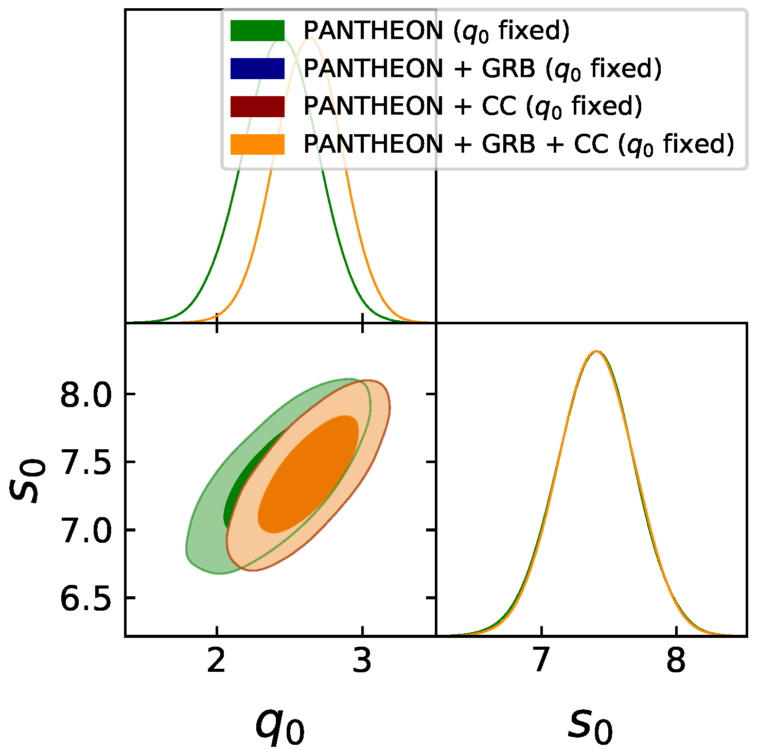
- Case (a). Fixed . Using the expression in Equation (35) and the values and (which relates to a pure power law in the boundary term theory), we obtain and , using the full Pantheon + GRB + CC using a Markov chain Monte Carlo (MCMC) analysis. For this case we obtain a Universe that is in decelerating phase. This sets the first constraint on the form of , where the cannot be fixed if we need to follow the correct cosmic acceleration. See Figure 1 for the posterior plot. Notice that once we add GRB we obtain the confidence level (C.L) overlaps on the Pantheon solely.
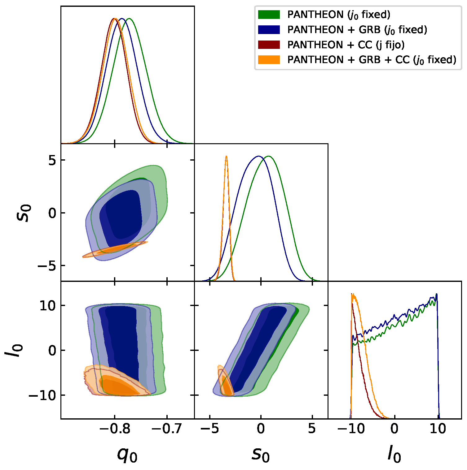
- Case (b). Fixed . Using the expression for j (37) and the values and , we obtain , , and using the full sample Pantheon + GRB+ CC with an MCMC analysis. For this case we obtain a Universe that is in fact accelerating as expected. See Figure 2 for details of the posterior. Here, we notice that the values of the higher derivative cosmographic parameters start to become reasonable.
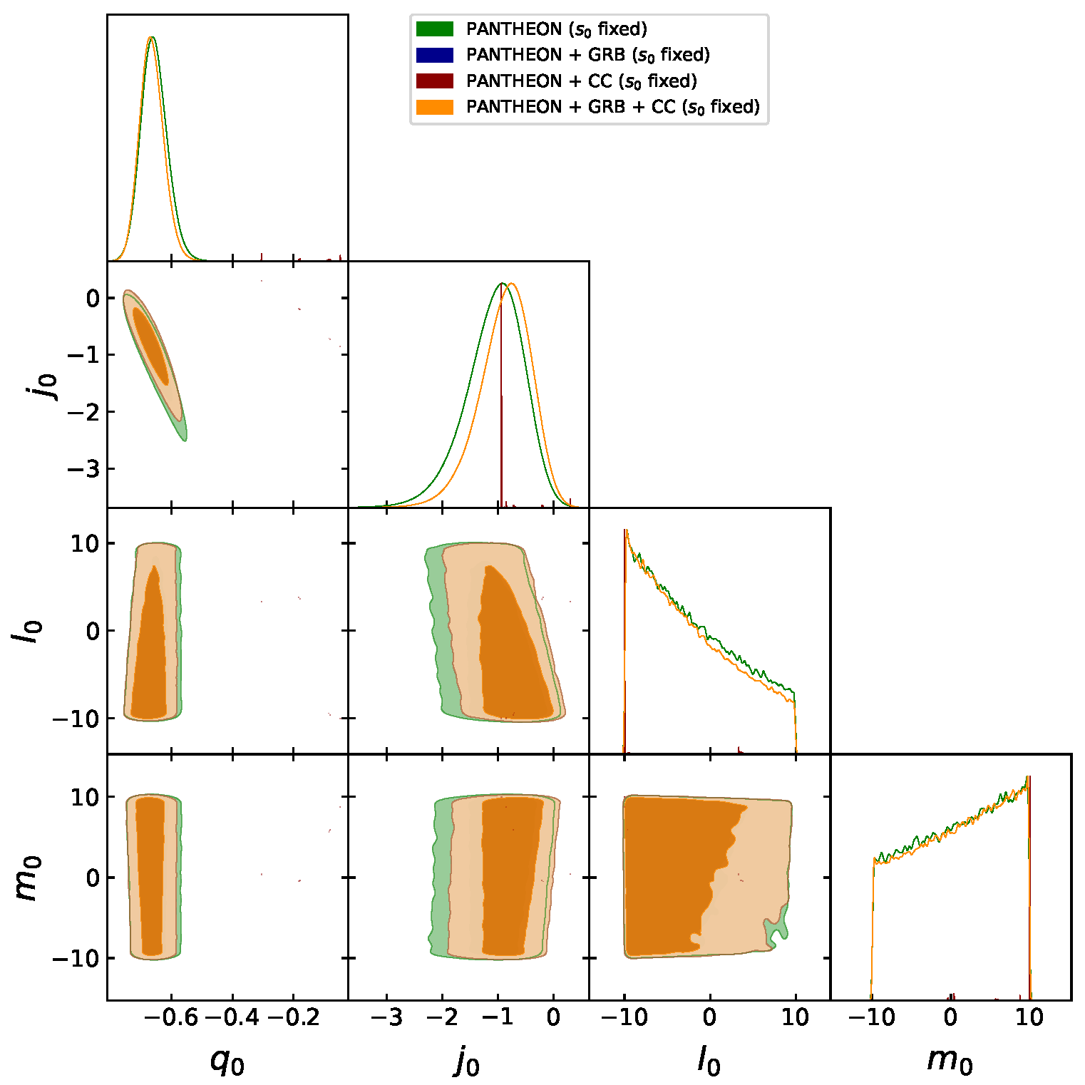
- Case (c). Fixed . Using the expression for s (37) and the values and , we obtain , , and using the full sample Pantheon + GRB+ CC. Notice that here the cosmography can go beyond . For this case we obtain a Universe that is in fact accelerating as expected and the addition of GRB explore the necessity of a high cosmography. See Figure 3.
In Table 1, we show the results of the MCMC analyses using both SN+CC and SN+CC+GRB data set compilations together with the three cases considered above for the cosmographic parameters. What we find is that due to the inter-relatedness of the cosmographic parameters, some high order derivative terms cannot be constrained such as which is due to the high degree of interdependence of the parameters. In this context, it follows suit that we can only consider a certain number of parameters depending on the amount of data available. Another important point concerns which parameters can be left fixed and which need to be constrained. In this analysis, we find that it is best to fix the highest derivative term and constrain the lower parameters, which leads to the best fit cosmographic parameters.
5. Conclusions and Discussion
Cosmography was used in this work to reconstruct elements of the Lagrangian in the context of a power law model. The cosmographic parameters (15) and (16) provide an interesting avenue to parameterizing the evolution of the Universe using progressively higher order derivative terms in the scale factor. Since they build on each other, these parameters can be related to each other which causes complicated coupling problems in many cases. For this reason, very high order derivative terms need enormous amounts of data to be constrained to any degree using observational data. On the other hand, these state parameters provide an efficient way to connect expansion terms with derivatives in a cosmological model.
In the context of TG, the cosmographic parameters can readily be injected into the scalar contributors of the theory (22). As expected progressively higher time derivatives of these scalar are naturally related to higher time derivatives of the Hubble parameter which is a crucial link with observations. Thus, using the Friedmann equations, the cosmographic parameters can then be related to the form of using the Friedmann equations which is the point at which this becomes dependent on the particular model under consideration (28)–(32). The other key property to acknowledge at this point is that it is not possible to isolate any of these cosmographic parameters for most model parameter values except for very specially chosen ones as explored in Case A in Equation (34). To this end, we use the luminosity distance calculation to strengthen the link to observations using the SN data set since it can be related to the distance modulus parameter, which is the true parameter of the Pantheon data set.
In Section 4, we consider the CC, SN and the new GRB data sets. GRB data are very interesting because they may shed new light on fundamental theory using new physical phenomena. To probe these potential differences, we consider three settings of cosmographic parameters in Figure 1, Figure 2 and Figure 3 which respectively constraint the cosmographic parameters for fixed , and . However, it is not possible in any of these analyses to completely constrain the value of high derivative terms such as the lerk l. Saying that, as more parameters are not fixed to a value, their values tend to the literature values such as in the case of the deceleration parameter which readily turns from a late-time decelerating solution in Figure 1 to an accelerating one in Figure 2 and Figure 3. The complete set of results are collected in Table 1 where the impact of the GRB data on the various cosmographic parameter is shown more clearly such as its preference for a weaker acceleration in the late Universe.
It would be interesting to consider other viable models in the gravity extension to CDM such as those models as proposed in Ref. [44]. However, it would make the analysis much more involved. It would also be advantageous to consider other approaches to constraining the evolution of the cosmographic parameters such as the non-parametric ones proposed in Refs. [75,76,77].
Author Contributions
All authors have contribute in all sections. All authors have read and agreed to the published version of the manuscript.
Funding
C.E.-R. and G.R.-F. are supported by DGAPA-PAPIIT-UNAM Project IA100220 and TA100122. GRF acknowledges financial support from CONACyT postgraduate grants program. J.L.-S. would also like to acknowledge funding support from Cosmology@MALTA which is supported by the University of Malta.
Acknowledgments
C.E.-R. acknowledges the Royal Astronomical Society as FRAS 10147. The simulations were performed in Centro de cómputo Tochtli-ICN-UNAM as part of CosmoNag ICN UNAM. The authors would like to acknowledge networking support by the COST Action CA18108.
Conflicts of Interest
The authors declare no conflict of interest.
Appendix A. Derivations for the Power Law Model Cosmography
As we mentioned, consider a simple model as a power law model , where mixed partial derivatives vanish and it can be seen that its derivatives are given by the following expressions:
These derivatives can be written in terms of the cosmographic parameters (15) and (16) using the expressions in (22) as:
Appendix B. Phenomenological Considerations
In this work we considered beforehand the model with . This model is too complex to be generally analysed in the context of cosmography, hence, we decided to work with one of the simplest form of these kind of models, the model where , and , which basically makes the functional to be . Although this model can be somehow justified from a theoretical point of view (in the sense that it is a simple extension of TEGR), it suffers from an ill phenomenology. Let us see this in detail.
The first modified Friedman equation in with the signature is given by (see Equation (19) in [44])
Since the boundary term and the torsion scalar are and respectively, the Equation (A23) can be rewritten as
Consider the model , which is exactly the same used here if . With this model, the Equation (A24) becomes
Using the Equation (22), the form of T and B, the Equation (A25) evaluated at is
which can be solved in terms of as
or from the amplitude coefficient equation as
If we substitute which corresponds to our simplified model and the values of the cosmographic parameters corresponding to CDM (, and ), the density parameter is
On the other hand, if we substitute , , and into (A28), the amplitude coefficient is
Hence, even though the model can recover a reasonable set of values for the cosmographic parameters, it is not completely phenomenological correct since it leads to a wrong value of the critical matter density parameter. On the other hand, this model does have some motivation from observational constraint analysis [44].
References
- Dodelson, S. Modern Cosmology; Academic Press: Cambridge, MA, USA, 2003. [Google Scholar]
- Weinberg, S. Gravitation and Cosmology: Principles and Applications of the General Theory of Relativity; John Wiley and Sons: Hoboken, NJ, USA, 1972. [Google Scholar]
- Riess, A.G.; Filippenko, A.V.; Challis, P.; Clocchiatti, A.; Diercks, A.; Garnavich, P.M.; Gilliland, R.L.; Hogan, C.J.; Jha, S.; Kirshner, R.P.; et al. Observational evidence from supernovae for an accelerating universe and a cosmological constant. Astron. J. 1998, 116, 1009–1038. [Google Scholar] [CrossRef] [Green Version]
- Perlmutter, S.; Aldering, G.; Goldhaber, G.; Knop, R.A.; Nugent, P.; Castro, P.G.; Deustua, S.; Fabbro, S.; Goobar, A.; Groom, D.E. Measurements of Omega and Lambda from 42 high redshift supernovae. Astrophys. J. 1999, 517, 565–586. [Google Scholar] [CrossRef]
- Binney, J. Galactic Dynamics/James Binney and Scott Tremaine, 2nd ed.; Princeton Series in Astrophysics; Princeton University Press: Princeton, NJ, USA, 2008. [Google Scholar]
- Bernal, J.L.; Verde, L.; Riess, A.G. The trouble with H0. J. Cosmol. Astropart. Phys. 2016, 10, 19. [Google Scholar] [CrossRef] [Green Version]
- Di Valentino, E.; Anchordoqui, L.A.; Akarsu, O.; Ali-Haimoud, Y.; Amendola, L.; Arendse, N.; Asgari, M.; Ballardini, M.; Basilakos, S.; Battistelli, E. Snowmass2021-Letter of interest cosmology intertwined II: The hubble constant tension. Astropart. Phys. 2021, 131, 102605. [Google Scholar] [CrossRef]
- Di Valentino, E.; Mena, O.; Pan, S.; Visinelli, L.; Yang, W.; Melchiorri, A.; Mota, D.F.; Riess, A.G.; Silk, J. In the realm of the Hubble tension—A review of solutions. Class. Quant. Grav. 2021, 38, 153001. [Google Scholar] [CrossRef]
- Aghanim, N.; Ashdown, M.; Aumont, J.; Baccigalupi, C.; Ballardini, M.; Banday, A.J.; Barreiro, R.B.; Bartolo, N.; Basak, S.; Battye, R.; et al. Planck 2018 results. VI. Cosmological parameters. arXiv 2018, arXiv:1807.06209. [Google Scholar]
- Di Valentino, E.; Anchordoqui, L.A.; Akarsu, O.; Ali-Haimoud, Y.; Amendola, L.; Arendse, N.; Asgari, M.; Ballardini, M.; Basilakos, S.; Battistelli, E. Cosmology intertwined III: fσ8 and S8. Astropart. Phys. 2021, 131, 102604. [Google Scholar] [CrossRef]
- Weinberg, S. The Cosmological Constant Problem. Rev. Mod. Phys. 1989, 61, 1–23. [Google Scholar] [CrossRef]
- Appleby, S.; Linder, E.V. The Well-Tempered Cosmological Constant. J. Cosmol. Astropart. Phys. 2018, 7, 34. [Google Scholar] [CrossRef] [Green Version]
- Gaitskell, R. Direct detection of dark matter. Ann. Rev. Nucl. Part. Sci. 2004, 54, 315–359. [Google Scholar] [CrossRef] [Green Version]
- Baudis, L. Dark matter detection. J. Phys. G 2016, 43, 044001. [Google Scholar] [CrossRef]
- Bertone, G.; Hooper, D.; Silk, J. Particle dark matter: Evidence, candidates and constraints. Phys. Rept. 2005, 405, 279–390. [Google Scholar] [CrossRef] [Green Version]
- Barboza, E.M., Jr.; Alcaniz, J.S. A parametric model for dark energy. Phys. Lett. B 2008, 666, 415–419. [Google Scholar] [CrossRef]
- Jassal, H.K.; Bagla, J.S.; Padmanabhan, T. Observational constraints on low redshift evolution of dark energy: How consistent are different observations? Phys. Rev. D 2005, 72, 103503. [Google Scholar] [CrossRef] [Green Version]
- Efstathiou, G. Constraining the equation of state of the universe from distant type Ia supernovae and cosmic microwave background anisotropies. Mon. Not. R. Astron. Soc. 1999, 310, 842–850. [Google Scholar] [CrossRef] [Green Version]
- Linder, E.V. Exploring the expansion history of the universe. Phys. Rev. Lett. 2003, 90, 091301. [Google Scholar] [CrossRef] [PubMed] [Green Version]
- Astier, P. Can luminosity distance measurements probe the equation of state of dark energy. Phys. Lett. B 2001, 500, 8–15. [Google Scholar] [CrossRef] [Green Version]
- Cooray, A.R.; Huterer, D. Gravitational lensing as a probe of quintessence. Astrophys. J. Lett. 1999, 513, L95–L98. [Google Scholar] [CrossRef] [Green Version]
- Escamilla-Rivera, C.; Nájera, A. Dynamical dark energy models in the light of Gravitational-Wave Transient Catalogues. arXiv 2021, arXiv:2103.02097. [Google Scholar]
- Colgáin, E.O.; Sheikh-Jabbari, M.M.; Yin, L. Can dark energy be dynamical? Phys. Rev. D 2021, 104, 023510. [Google Scholar] [CrossRef]
- Clifton, T.; Ferreira, P.G.; Padilla, A.; Skordis, C. Modified Gravity and Cosmology. Phys. Rept. 2012, 513, 1–189. [Google Scholar] [CrossRef] [Green Version]
- Capozziello, S.; De Laurentis, M. Extended Theories of Gravity. Phys. Rept. 2011, 509, 167–321. [Google Scholar] [CrossRef] [Green Version]
- Saridakis, E.N.; Lazkoz, R.; Salzano, V.; Moniz, P.V.; Capozziello, S.; Jiménez, J.B.; De Laurentis, M.; Olmo, G.J.; Akrami, Y.; Bahamonde, S. Modified Gravity and Cosmology: An Update by the CANTATA Network. arXiv 2021, arXiv:2105.12582. [Google Scholar]
- Bamba, K.; Capozziello, S.; Nojiri, S.; Odintsov, S.D. Dark energy cosmology: The equivalent description via different theoretical models and cosmography tests. Astrophys. Space Sci. 2012, 342, 155–228. [Google Scholar] [CrossRef] [Green Version]
- Yang, T.; Banerjee, A.; Colgáin, E.O. Cosmography and flat ΛCDM tensions at high redshift. Phys. Rev. D 2020, 102, 123532. [Google Scholar] [CrossRef]
- Bahamonde, S.; Dialektopoulos, K.F.; Escamilla-Rivera, C.; Farrugia, G.; Gakis, V.; Hendry, M.; Hohmann, M.; Said, J.L.; Mifsud, J.; Di Valentino, E. Teleparallel Gravity: From Theory to Cosmology. arXiv 2021, arXiv:2106.13793. [Google Scholar]
- Aldrovandi, R.; Pereira, J.G. Teleparallel Gravity; Springer: Dordrecht, The Netherlands, 2013; Volume 173. [Google Scholar] [CrossRef]
- Cai, Y.F.; Capozziello, S.; De Laurentis, M.; Saridakis, E.N. f(T) teleparallel gravity and cosmology. Rept. Prog. Phys. 2016, 79, 106901. [Google Scholar] [CrossRef] [Green Version]
- Krssak, M.; van den Hoogen, R.; Pereira, J.; Böhmer, C.; Coley, A. Teleparallel theories of gravity: Illuminating a fully invariant approach. Class. Quant. Grav. 2019, 36, 183001. [Google Scholar] [CrossRef] [Green Version]
- Lovelock, D. The Einstein tensor and its generalizations. J. Math. Phys. 1971, 12, 498–501. [Google Scholar] [CrossRef]
- Gonzalez, P.; Vasquez, Y. Teleparallel Equivalent of Lovelock Gravity. Phys. Rev. D 2015, 92, 124023. [Google Scholar] [CrossRef] [Green Version]
- Bahamonde, S.; Dialektopoulos, K.F.; Levi Said, J. Can Horndeski Theory be recast using Teleparallel Gravity? Phys. Rev. D 2019, 100, 064018. [Google Scholar] [CrossRef] [Green Version]
- Sotiriou, T.P.; Faraoni, V. f(R) Theories Of Gravity. Rev. Mod. Phys. 2010, 82, 451–497. [Google Scholar] [CrossRef] [Green Version]
- Faraoni, V. f(R) gravity: Successes and challenges. In Proceedings of the 18th SIGRAV Conference, Urbino, Italy, 9–15 September 2008. [Google Scholar]
- Ferraro, R.; Fiorini, F. Modified teleparallel gravity: Inflation without inflaton. Phys. Rev. D 2007, 75, 084031. [Google Scholar] [CrossRef] [Green Version]
- Ferraro, R.; Fiorini, F. On Born-Infeld Gravity in Weitzenbock spacetime. Phys. Rev. D 2008, 78, 124019. [Google Scholar] [CrossRef] [Green Version]
- Bengochea, G.R.; Ferraro, R. Dark torsion as the cosmic speed-up. Phys. Rev. D 2009, 79, 124019. [Google Scholar] [CrossRef] [Green Version]
- Linder, E.V. Einstein’s Other Gravity and the Acceleration of the Universe. Phys. Rev. D 2010, 81, 127301. [Google Scholar] [CrossRef] [Green Version]
- Chen, S.H.; Dent, J.B.; Dutta, S.; Saridakis, E.N. Cosmological perturbations in f(T) gravity. Phys. Rev. D 2011, 83, 023508. [Google Scholar] [CrossRef] [Green Version]
- Bahamonde, S.; Flathmann, K.; Pfeifer, C. Photon sphere and perihelion shift in weak f(T) gravity. Phys. Rev. D 2019, 100, 084064. [Google Scholar] [CrossRef] [Green Version]
- Escamilla-Rivera, C.; Levi Said, J. Cosmological viable models in f(T, B) gravity as solutions to the H0 tension. Class. Quant. Grav. 2020, 37, 165002. [Google Scholar] [CrossRef]
- Bahamonde, S.; Böhmer, C.G.; Wright, M. Modified teleparallel theories of gravity. Phys. Rev. D 2015, 92, 104042. [Google Scholar] [CrossRef]
- Capozziello, S.; Capriolo, M.; Transirico, M. The gravitational energy-momentum pseudotensor: The cases of f(R) and f(T) gravity. Int. J. Geom. Meth. Mod. Phys. 2018, 15, 1850164. [Google Scholar] [CrossRef] [Green Version]
- Bahamonde, S.; Capozziello, S. Noether Symmetry Approach in f(T, B) teleparallel cosmology. Eur. Phys. J. C 2017, 77, 107. [Google Scholar] [CrossRef] [PubMed] [Green Version]
- Paliathanasis, A. de Sitter and Scaling solutions in a higher-order modified teleparallel theory. J. Cosmol. Astropart. Phys. 2017, 1708, 027. [Google Scholar] [CrossRef] [Green Version]
- Farrugia, G.; Levi Said, J.; Gakis, V.; Saridakis, E.N. Gravitational Waves in Modified Teleparallel Theories. Phys. Rev. D 2018, 97, 124064. [Google Scholar] [CrossRef] [Green Version]
- Bahamonde, S.; Zubair, M.; Abbas, G. Thermodynamics and cosmological reconstruction in f(T, B) gravity. Phys. Dark Univ. 2018, 19, 78–90. [Google Scholar] [CrossRef] [Green Version]
- Wright, M. Conformal transformations in modified teleparallel theories of gravity revisited. Phys. Rev. D 2016, 93, 103002. [Google Scholar] [CrossRef] [Green Version]
- Farrugia, G.; Levi Said, J.; Finch, A. Gravitoelectromagnetism, Solar System Test and Weak-Field Solutions in f(T, B) Gravity with Observational Constraints. Universe 2020, 6, 34. [Google Scholar] [CrossRef] [Green Version]
- Capozziello, S.; Capriolo, M.; Caso, L. Weak Field Limit and Gravitational Waves in f(T, B) Teleparallel Gravity. Eur. Phys. J. C 2020, 80, 156. [Google Scholar] [CrossRef] [Green Version]
- Bahamonde, S.; Levi Said, J.; Zubair, M. Solar System Tests in Modified Teleparallel Gravity. arXiv 2020, arXiv:2006.06750. [Google Scholar] [CrossRef]
- Hehl, F.W.; Von Der Heyde, P.; Kerlick, G.D.; Nester, J.M. General Relativity with Spin and Torsion: Foundations and Prospects. Rev. Mod. Phys. 1976, 48, 393–416. [Google Scholar] [CrossRef] [Green Version]
- Hohmann, M. Variational Principles in Teleparallel Gravity Theories. Universe 2021, 7, 114. [Google Scholar] [CrossRef]
- Weitzenböock, R. Invariantentheorie; Noordhoff: Gronningen, The Netherlands, 1923. [Google Scholar]
- Ortín, T. Gravity and Strings; Cambridge Monographs on Mathematical Physics; Cambridge University Press: Cambridge, UK, 2004. [Google Scholar]
- Zubair, M.; Durrani, L.R.; Waheed, S. Reconciling Tsallis holographic dark energy models in modified f(T, B) gravitational framework. Eur. Phys. J. Plus 2021, 136, 943. [Google Scholar] [CrossRef]
- Zubair, M.; Durrani, L.R. A study of the cosmologically reconstructed f(T, B) gravity from the cosmological jerk parameter. Eur. Phys. J. Plus 2020, 135, 668. [Google Scholar] [CrossRef]
- Zubair, M.; Waheed, S.; Atif Fayyaz, M.; Ahmad, I. Energy constraints and the phenomenon of cosmic evolution in the f(T, B) framework. Eur. Phys. J. Plus 2018, 133, 452. [Google Scholar] [CrossRef] [Green Version]
- Krššák, M.; Saridakis, E.N. The covariant formulation of f(T) gravity. Class. Quant. Grav. 2016, 33, 115009. [Google Scholar] [CrossRef] [Green Version]
- Tamanini, N.; Boehmer, C.G. Good and bad tetrads in f(T) gravity. Phys. Rev. D 2012, 86, 044009. [Google Scholar] [CrossRef] [Green Version]
- Capozziello, S.; Cardone, V.F.; Farajollahi, H.; Ravanpak, A. Cosmography in f(T)-gravity. Phys. Rev. D 2011, 84, 043527. [Google Scholar] [CrossRef] [Green Version]
- Aviles, A.; Gruber, C.; Luongo, O.; Quevedo, H. Cosmography and constraints on the equation of state of the Universe in various parametrizations. Phys. Rev. D 2012, 86, 123516. [Google Scholar] [CrossRef] [Green Version]
- Franco, G.A.R.; Escamilla-Rivera, C.; Levi Said, J. Stability analysis for cosmological models in f(T, B) gravity. Eur. Phys. J. C 2020, 80, 677. [Google Scholar] [CrossRef]
- Caruana, M.; Farrugia, G.; Levi Said, J. Cosmological bouncing solutions in f(T, B) gravity. Eur. Phys. J. C 2020, 80, 640. [Google Scholar] [CrossRef]
- Bahamonde, S.; Golovnev, A.; Guzmán, M.J.; Said, J.L.; Pfeifer, C. Black Holes in f(T, B) Gravity: Exact and Perturbed Solutions. arXiv 2021, arXiv:2110.04087. [Google Scholar]
- Scolnic, D.M.; Jones, D.O.; Rest, A.; Pan, Y.C.; Chornock, R.; Foley, R.J.; Huber, M.E.; Kessler, R.; Narayan, G.; Riess, A.G.; et al. The Complete Light-curve Sample of Spectroscopically Confirmed SNe Ia from Pan-STARRS1 and Cosmological Constraints from the Combined Pantheon Sample. Astrophys. J. 2018, 859, 101. [Google Scholar] [CrossRef]
- Qi, S.; Lu, T. A new luminosity relation for gamma-ray bursts and its implication. Astrophys. J. 2010, 717, 1274–1278. [Google Scholar] [CrossRef]
- Wang, Y.Y.; Wang, F.Y. Calibration of Gamma-Ray Burst Luminosity Correlations Using Gravitational Waves as Standard Sirens. Astrophys. J. 2019, 873, 39. [Google Scholar] [CrossRef] [Green Version]
- Escamilla-Rivera, C.; Carvajal, M.; Zamora, C.; Hendry, M. Neural networks and standard cosmography with newly calibrated high redshift GRB observations. arXiv 2021, arXiv:2109.00636. [Google Scholar]
- D’Agostini, G. Fits, and especially linear fits, with errors on both axes, extra variance of the data points and other complications. arXiv 2005, arXiv:physics/0511182. [Google Scholar]
- Jimenez, R.; Loeb, A. Constraining cosmological parameters based on relative galaxy ages. Astrophys. J. 2002, 573, 37–42. [Google Scholar] [CrossRef]
- Escamilla-Rivera, C.; Levi Said, J.; Mifsud, J. Performance of Non-Parametric Reconstruction Techniques in the Late-Time Universe. arXiv 2021, arXiv:2105.14332. [Google Scholar] [CrossRef]
- Bernardo, R.C.; Levi Said, J. Towards a model-independent reconstruction approach for late-time Hubble data. J. Cosmol. Astropart. Phys. 2021, 08, 027. [Google Scholar] [CrossRef]
- Briffa, R.; Capozziello, S.; Levi Said, J.; Mifsud, J.; Saridakis, E.N. Constraining teleparallel gravity through Gaussian processes. Class. Quant. Grav. 2020, 38, 055007. [Google Scholar] [CrossRef]
Figure 1.
Case (a) using Pantheon compilation (green C.L.), Pantheon+GRB (blue C.L.), Pantheon+CC (red C.L.) and Pantheon+GRB+CC (orange C.L.).
Figure 1.
Case (a) using Pantheon compilation (green C.L.), Pantheon+GRB (blue C.L.), Pantheon+CC (red C.L.) and Pantheon+GRB+CC (orange C.L.).

Figure 2.
Case (b) using Pantheon compilation (green C.L.), Pantheon+GRB (blue C.L.), Pantheon+CC (red C.L.) and Pantheon+GRB+CC (orange C.L.).
Figure 2.
Case (b) using Pantheon compilation (green C.L.), Pantheon+GRB (blue C.L.), Pantheon+CC (red C.L.) and Pantheon+GRB+CC (orange C.L.).

Figure 3.
Case (c) using Pantheon compilation (green C.L.), Pantheon+GRB (blue C.L.), Pantheon+CC (red C.L.) and Pantheon+GRB+CC (orange C.L.).
Figure 3.
Case (c) using Pantheon compilation (green C.L.), Pantheon+GRB (blue C.L.), Pantheon+CC (red C.L.) and Pantheon+GRB+CC (orange C.L.).


Table 1.
Best cosmographic fits for the standard case using a power law model. In first columns are denoted the three cases considered. We divided the analysis using: Pantheon SN + CC (second block column) and Pantheon SN + CC + GRB (third block column). The word fixed indicates a flat CDM prior imposed on each case. Results are discussed in the text.
| Cases | Pantheon SN + CC | Pantheon SN + CC + GRB | ||||||||
|---|---|---|---|---|---|---|---|---|---|---|
| (a) | Fixed | - | - | Fixed | - | - | ||||
| (b) | Fixed | - | Fixed | - | ||||||
| (c) | Fixed | Fixed | ||||||||
Publisher’s Note: MDPI stays neutral with regard to jurisdictional claims in published maps and institutional affiliations. |
© 2021 by the authors. Licensee MDPI, Basel, Switzerland. This article is an open access article distributed under the terms and conditions of the Creative Commons Attribution (CC BY) license (https://creativecommons.org/licenses/by/4.0/).
Share and Cite
MDPI and ACS Style
Escamilla-Rivera, C.; Rave-Franco, G.; Levi-Said, J. f(T, B) Cosmography for High Redshifts. Universe 2021, 7, 441. https://0-doi-org.brum.beds.ac.uk/10.3390/universe7110441
AMA Style
Escamilla-Rivera C, Rave-Franco G, Levi-Said J. f(T, B) Cosmography for High Redshifts. Universe. 2021; 7(11):441. https://0-doi-org.brum.beds.ac.uk/10.3390/universe7110441
Chicago/Turabian StyleEscamilla-Rivera, Celia, Geovanny Rave-Franco, and Jackson Levi-Said. 2021. "f(T, B) Cosmography for High Redshifts" Universe 7, no. 11: 441. https://0-doi-org.brum.beds.ac.uk/10.3390/universe7110441
Note that from the first issue of 2016, this journal uses article numbers instead of page numbers. See further details here.