
Global Dynamics of the Hořava–Lifshitz Cosmological Model in a Non-Flat Universe with Non-Zero Cosmological Constant


1
School of Mathematical Science, Yangzhou University, Yangzhou 225002, China
2
Departament de Matemàtiques, Universitat Autònoma de Barcelona, Bellaterra, 08193 Barcelona, Spain
*
Author to whom correspondence should be addressed.
Universe 2021, 7(11), 445; https://0-doi-org.brum.beds.ac.uk/10.3390/universe7110445
Submission received: 20 October 2021
/
Revised: 13 November 2021
/
Accepted: 15 November 2021
/
Published: 17 November 2021
(This article belongs to the Section Cosmology)
Abstract
:When the cosmological constant is non-zero, the dynamics of the cosmological model based on Hořava–Lifshitz gravity in a non-flat universe are characterized by using the qualitative theory of differential equations.
1. Introduction
After the Newtonian era, Einstein put forward the general theory of relativity, and this gave our understanding of gravity, once again, a huge leap forward. In 2009 Hořava proposed a non-relativistic theory of renormalizable gravity [1], which can be reduced to Einstein’s general theory of relativity on a large scale. It is named Hořava–Lifshitz gravity together with the scalar field theory of Lifshitz. This theory has inspired many studies and applications in length renormalization [2], entropy argument [3], cosmology [4,5,6,7,8,9,10,11,12,13,14,15,16,17,18,19,20,21,22,23,24,25,26,27,28,29,30], dark energy [31,32,33,34,35], black holes [36,37,38,39,40], gravitational waves [41] and electromagnetics [42,43,44,45]. More information can also be found in the review articles [46,47,48] and the references therein.
In the past ten years, Leon et al. [9,10,11,12] have conducted several excellent studies on the Hořava–Lifshitz cosmological model, whether the curvature k of the universe is zero and whether the cosmological constant should be considered. They divided the cosmological model into four types in the Friedmann–Lemaître–Robertson–Walker (FLRW) background spacetime: (1) ; (2) ; (3) ; (4) . By using the phase-space analysis, they discussed the two-dimensional dynamics of the Hořava–Lifshitz cosmological model under the usual exponential potential, and partially studied its three-dimensional dynamics.
For the important cosmological constant that many researchers have been paying attention to, this constant put the Hořava–Lifshitz gravitational theory in a delicate balance, which led to a conflict between its cosmology and observations. Appignani et al. [49] showed that the huge difference between the standard predictions from quantum field theory and the observed value of may have a solution in the Hořava–Lifshitz gravity framework. Akarsu et al. [50] investigated the in the standard cold dark matter model by introducing graduated dark energy. Their results provided a high probability that the sign of could be spontaneously converted, and inferred that the universe had transformed from anti-de Sitter vacua to de Sitter vacua and triggered late acceleration. Carlip [51] proposed that the vacuum fluctuations produce a huge and produce a high curvature k on the Planck scale under the standard effective field theory. Although the debate about the shape of the universe has not yet reached an agreement, for the boundaries of the universe are blurred, the odds are 50:1 that the universe is closed if the Planck CMB data are correct [52]. Besides, Valentino et al. [53] also believed that the universe could be a closed three-dimensional sphere, unlike the prediction from the standard cold dark matter model. The curvature can be positive according to the enhanced lensing amplitude in the cosmic microwave background power spectrum confirmed by the Planck Legacy 2018.
For the case , the global dynamics of the Hořava–Lifshitz scalar field cosmological model under the background of FLRW were described in [14,15], and the case of with zero curvature has also been addressed in [16]. In the present paper we discuss the global dynamics of a non-flat universe with . We provide detailed information on obtaining cosmological equations in Section 2.
2. The Cosmological Equations
In this section, we first briefly recall the classic Hořava–Lifshitz gravitational theory, where the field content can be represented by the space vector and scalar N, and they are common “lapse” and “shift” variables in general relativity [1,9,22]. Then the full metric can be defined as
where is a spatial metric. The rescaling conversion meets the conditions , under which and N remain unchanged, but is scaled to .
Under the detailed-balance condition, the full gravitational action of Hořava–Lifshitz is written as
where denotes the extrinsic curvature, represents the Cotton tensor and is the standard general covariant antisymmetric tensor. The indices are to raise and lower with the metric . The parameters , and w are constants (see [1] for more details).
For the potential we take into account the gravitational action term as follows:
and the metric , , . Here the function is the dimensionless rescaling factor of the expanding universe, and is a constant curvature metric of being maximally symmetric. Without loss of generality, we normalize and N to the number one, and then we can describe the cosmological model as
where is the Hubble parameter which gives the expansion rate of the universe.
Therefore, the field equations become the form of the following autonomous dynamical system.
where ; is a constant; is the usual scalar field potential, which admits various mathematical representations (see [11,13,18,19])—it can even be presented in a constant form in scalar cosmology ([20,21]); and s is assumed to be a constant under the usual exponential potentials. For more details on system (7), see Equation (5.72) of [10], or Equations (287)–(290) of [11], or Equations (59)–(61) of [12].
In this paper, we study the global dynamics of system (7) in the physical region of interest
where corresponding to a closed, flat and open universe, respectively. For the case , we note that is an invariant surface because there is a polynomial such that
The invariant surface here is essential for understanding the complex dynamic behavior of the model (7), because if a point on an orbit of system (7) is located on the invariant surface, then the whole orbit is contained in the surface. However, is not an invariant surface for the case . In addition, it is also noted that system (7) is invariant under the three symmetries and , if ; i.e. it is symmetric with respect to the x-axis, and additionally with respect to the origin and the plane when . Therefore, we divide the study of system (7) into four cases, taking into account the existence or not of the symmetric plane and of the invariant surface.
- Case I: and , so system (7) is symmetric with respect to the x-axis and it has the invariant surface .
- Case II: and , so system (7) is symmetric with respect to the x-axis and it has not the invariant surface.
- Case III: and , so system (7) is symmetric with respect to the origin and with respect to the x-axis, and it has the invariant surface .
- Case IV: and , so system (7) is symmetric with respect to the origin and with respect to the x-axis, and it has not the invariant surface.
In Section 3.1 we investigate the phase portraits of case I of system (7) on the invariant planes and surface, along with the local phase portraits at the finite and infinite equilibrium points. In Section 3.2 we discuss the phase portraits of case I of system (7) inside the Poincaré ball restricted to the region G. Based on these sections, considering the symmetry of system (7), we study the global dynamics of system (7), adding its behavior at infinity in Section 3.3. In Section 4 we study case II in the same way as in case I. In Section 5 and Section 6 we describe the global dynamics of system (7) in the closed and open universe models, respectively, when the field potential of the system takes the form of a constant, i.e. in cases III and IV. Moreover, we give the final discussion and summary in Section 7.
3. Case I:
3.1. Phase Portraits on the Invariant Planes and Surface
In order to analyze in detail the local phase portraits at the finite and infinite equilibrium points and the global phase portrait of system (7) in the region G (refer to [9,10,11] or [12] again), we first study its phase portraits on the invariant planes and , and on the invariant surface , respectively.
3.1.1. The Invariant Plane
On this plane system (7) becomes
There are three equilibrium points , and of system (8), where has eigenvalues 3 and ; has eigenvalues 3 and ; and has eigenvalues and .
Therefore, the equilibrium point is a hyperbolic unstable node when , and it is a hyperbolic unstable saddle when . The equilibrium point is a hyperbolic unstable node when , and it is a hyperbolic unstable saddle when . The equilibrium point is a hyperbolic unstable node when , and it is a hyperbolic unstable saddle when . Moreover, for , is a semi-hyperbolic saddle-node, by using the semi-hyperbolic singular point theorem (see Theorem 2.19 in [54] for more details). Similarly, for , is also a semi-hyperbolic saddle-node.
Since the types and stability of these three finite equilibrium points vary with the different values of s, we summarize them in Table 1.
By using the Poincaré compactification (see Chapter 5 of [54] for more details), it will help us realize how to draw the vector field of system (8) in the local charts and , and then we can determine how the orbits come from or go to infinity. On the local chart we let and ; then system (8) becomes
Then all the points of system (9) at infinity are equilibrium points, we rescale the time , so this system is
However, this system has no equilibrium points at infinity .
Similarly, on the local chart we have and ; thus, system (8) reduces to
On the local chart we only need to study the origin of system (11). Obviously is an equilibrium point. Since its linear part is identically zero, we cannot use the usual eigenvalue method to determine the type of the equilibrium point and its local phase portrait, but we note that the straight line of system (11) is full of equilibrium points, and if the common factor V in system (11) is eliminated, there are no other equilibrium points in . When , on the positive semi-axis of V, indicates that V decreases monotonically, and on the negative semi-axis of V, means that V increases monotonically. Near the straight line , , U increases monotonically when , and U decreases monotonically when . Therefore, the local phase portrait of the equilibrium point of system (11) is shown in Figure 1a when . Similarly, the local phase portrait of is illustrated in Figure 1b when .
Therefore, the corresponding global phase portrait of system (8) restricted to the region can be summarized in Figure 2.
3.1.2. The Invariant Plane
On this plane system (7) is
There are five equilibrium points, , , , and , in system (12) when , and the latter three equilibrium points, , and , coincide when . The equilibrium point has eigenvalues 1 and , it is a hyperbolic unstable node when , and it is a hyperbolic unstable saddle when . The equilibrium point has eigenvalues 1 and , it is a hyperbolic unstable node when , and it is a hyperbolic unstable saddle when . The equilibrium point has eigenvalues and , it is a hyperbolic unstable node when or , and it is a hyperbolic unstable saddle when . The equilibrium points and have the same eigenvalues and . They are hyperbolic unstable saddles when , and they are not real singularities when .
In addition, for the value , the equilibrium point is a semi-hyperbolic saddle-node by using the semi-hyperbolic singular point theorem. Similarly, for the value , the equilibrium point is also a semi-hyperbolic saddle-node. For the value , the equilibrium point is a semi-hyperbolic unstable saddle.
Since the types and stability of these five finite equilibrium points change with different values of s, we summarize them in Table 2.
By using the Poincaré compactification again on the local chart , the system (12) becomes
Hence, all the infinite points of system (13) are filled with equilibrium points at , doing the time rescaling yields
However, this system does not admit any equilibrium point on .
Similarly, on the local chart , system (12) reduces to
The origin of system (15) is a equilibrium point with eigenvalues 2 and 0, but it is not semi-hyperbolic because it is not isolated in the set of all equilibrium points. It is noted that the axis is full of equilibrium points of system (15). For the positive semi-axis of V near , means that V increases monotonically, and on the negative semi-axis of V, indicates that V decreases monotonically. Moreover, around the straight line , thus U increases monotonically when , and U decreases monotonically when . Therefore, the local phase portrait of the semi-hyperbolic equilibrium point in system (15) is illustrated in Figure 3a when . Similarly, the local phase portrait of is shown in Figure 3b for when .
Hence, the corresponding global phase portrait of system (12) restricted to the region is illustrated in Figure 4 and Figure 5. However, we need to pay attention that the global phase portrait of system (12) is similar when and (see Figure 4c,d). The main difference is that the equilibrium point is a hyperbolic unstable saddle when , while it is a semi-hyperbolic unstable saddle. The same situation occurs when and (see Figure 5b,c).
3.1.3. The Invariant Surface
Note that ; thus, for the case , system (16) admits two equilibrium points and . In addition we also note that system (16) is symmetric with respect to u-axis under the symmetry , so we only need to discuss the equilibrium point . However, the functions on the right side of system (16) have no derivative at , which means that the local dynamics near cannot be studied by the methods in the previous Section 3.1.1 and Section 3.1.2. When , the first equation in system (16) is always equal to zero, and the second equation is simplified to , i.e. on the invariant straight line the solution is (c is an arbitrary constant), which indicates that tends to infinity in forward time and leads to in backward time.
We know the dynamics on near , but we want to know the dynamics in a neighborhood of . To this end we set , i.e. , considering the aforementioned symmetry. We only discuss the case here, so system (9) can be rewritten as follows:
It is obvious that system (18) has a fictitious equilibrium point because , and its eigenvalues are 1 and 3, respectively, i.e. is a fictitious hyperbolic unstable node. The first equation of system (18) shows that when , so y increases monotonically. In contrast, if , then y decreases monotonically. Note that x and y have the same monotonicity when , so the local phase portrait of system (16) near and system (18) near have the same local phase portrait. Then considering the symmetry of system (18), we can find that the local phase portrait of system (16) is shown in Figure 6.
Similarly, the local phase portrait of system (17) is shown in Figure 7.
Note that system (16) can be transformed into a polynomial differential system by letting when . In order to study the dynamic behavior of the equilibrium points of system (16) at infinity, we first study the infinite equilibrium points of system (18). On the local chart system (18) is
It is easy to find that all the infinite points of system (19) at are equilibrium points. Performing time scale transformation to eliminate the common factor V in system (19) gives
This system has a unique equilibrium point in , with eigenvalues , it is a hyperbolic saddle.
On the local chart system (18) reads
Using time rescaling we obtain
The origin is an equilibrium point, which is a hyperbolic stable center with eigenvalue (i is the imaginary unit). Hence is either a weak focus or a center, but since is a first integral of system (22) defined at , is a center. Then the global phase portrait of system (18) with is shown in Figure 8.
3.1.4. The Finite Equilibrium Points
It is easy to find that there are five finite equilibrium points of system (7) because in case I. The equilibrium point with eigenvalues 3, 1 and , the equilibrium point with eigenvalues 3, 1 and , the equilibrium points , , and have the same eigenvalues 2, and , and the equilibrium point with eigenvalues , and . Since different values of s determine the types of these five equilibrium points, we list the relevant results more clearly in Table 3.
3.1.5. Phase Portrait on the Poincaré Sphere at Infinity
According to the three-dimensional Poincaré compactification (see [55] for more details), we set . Thus, on the local chart , system (7) is rewritten as
Since the infinity at the different local charts of Poincaré sphere corresponds to , then for all , system (23) has the equilibrium point with eigenvalues , which means that the local chart are full of equilibrium points at infinity. Note that the corresponding eigenvectors are
By using normally hyperbolic submanifold theorem (see Appendix A for details), the equilibrium point has a one-dimensional stable manifold when and unstable when . More details are shown in regions I, II, and III of Figure 11. However, for the equilibrium points on the hyperbola there are six local phase portraits in Figure 12. Note that there is one-dimensional stable manifold in region I and one-dimensional unstable manifold in regions II and III filled with infinite equilibrium points. Since the orbits arriving or ending at equilibrium points at infinity in the different regions cannot collide into finite equilibrium points when they tend to equilibrium points on the hyperbola coming from both sides of this hyperbola, there is a hyperbolic sector on the equilibrium points of the branches and of the hyperbola, with the exception of two points and ; see the first two pictures in Figure 12 for details.
Doing time rescaling system (23) becomes
At system (25) has two lines filled with infinite equilibrium points and these two lines intersect with hyperbola at and , respectively. Both of them are hyperbolic with the same eigenvalues and the corresponding eigenvectors have the following form:
Then and have an unstable manifold of dimension one (respectively two) and a stable manifold of dimension two (respectively one) if (respectively ); see the last four pictures in Figure 12 for details.
On the local chart , we let . Thus, system (7) is
By eliminating the common factor in system (27) through time scale transformation we get
Note that system (28) with has the unique infinite equilibrium point with eigenvalues {2i, -2i, 0} and eigenvectors {0, -i, 1}, {0, i, 1}, {1, 0, 0}, so there will be a fold-Hopf bifurcation at the infinite equilibrium point , sometimes called a zero-pair bifurcation or a Gavrilov-Guckenheimer (see Chapter 5 of [56] for more details). We will not continue to discuss other infinite equilibrium points of this system, because these are already included in the local chart .
Similarly, on the local chart , we let , so system (7) becomes
In this local chart we only need to study the infinite equilibria located in its origin because all the other infinite equilibrium points have been studied in the local charts and . After changing the time scale we obtain
Obviously the origin is not an equilibrium point of system (30), so we will not continue to investigate other equilibrium points at infinity in the local chart .
3.2. Phase Portrait Inside the Poincaré Ball Restricted to the Physical Region of Interest
Note that system (7) is invariant with respect to the x-axis due to the symmetry . Now we divide the Poincaré ball restricted to the region into four regions as follows:
Due to the symmetry with respect to the x-axis, we only need to discuss the phase portrait of system (7) in the regions and .
Combining the phase portraits on the invariant surface , on the invariant planes and , and at infinity, we obtain the phase portrait on the boundary of the regions and as shown in Figure 14, Figure 15, Figure 16 and Figure 17.
Now as shown in Figure 18 and Figure 19, we divided the boundary of the regions and into sub-surfaces , , ⋯ and ; and , , ⋯, , respectively. Thus, the phase portrait on the boundary of could be displayed more clearly. Therefore, we can find from Figure 13, Figure 15 and Figure 17 that there is a hyperbolic sector at the north pole N on spherical boundary of the Poincaré ball, and N is stable on the back boundary plane . The equilibrium points and are unstable on the boundary surfaces . Moreover, the equilibrium point is unstable on the back boundary planes and , and it is stable on the bottom boundary planes and and at their intersection. In addition the properties of the remaining equilibrium points that are not located at the intersection of these boundary surfaces and planes have been studied in the previous section and will not be repeated here.
3.3. Dynamics in the Interior of the Regions and
Without loss of generality and considering the physical region of interest, we take , and the dynamics of system (7) can be studied in the same way when we take other values of s. Then the five finite equilibrium points of system (7) have the form , , , and . The dynamical behavior of system (7) inside the region is determined by the behavior of the flow in the following planes and surfaces:
where
The above planes and surfaces divide the regions and into eleven subregions and nine subregions , respectively; see Figure 20, Figure 21, Figure 22 and Figure 23 for more details. The signs of the functions , and in these subregions of and can be found in Table 4 and Table 5, respectively.
In addition it should also be noted that in order to avoid visual confusion, we change the dashed lines and solid lines in Figure 21 and Figure 23 to the normal perspective, instead of corresponding to the dashed lines and solid lines in Figure 20 and Figure 22, respectively. What we need to pay attention here is that for any value of s, the finite equilibrium point is located at the intersection of the surfaces and on the invariant plane , and the finite equilibrium point is located at the intersection of the surface and x-axis (see Figure 21 and Figure 23). For the infinite equilibrium point of Equations (25), according to the three-dimensional Poincaré transformation in the local chart , we know that is on the intersection of the surface and the Poincaré sphere. Similarly, in the coordinate system we have , since the infinite equilibrium points and are symmetric about the origin, then we obtain , which is symmetric with with respect to the plane . For the infinite equilibrium point of equations (20) when , we combine the relationship in equations (18) and the invariant surface to know that the coordinate of in the three-dimensional coordinate system can be denoted as , obviously the infinite equilibrium point is not in the region . However, when we have , and it is exactly located on the surface , on the invariant surface and in their intersection with the Poincaré sphere (see Figure 21).
As it is shown in the subregion (see Figure 21) the left side surface is contained in the invariant surface , the bottom plane is contained in the invariant plane , the right-back segment surface is contained in and the right-front segment surface is contained in . From Table 6 we find that the orbits of system (7) increase monotonically along the positive directions of the three coordinate axes, which means that the orbits in come from the finite equilibrium points and , or from the subregion , and then go to the boundary of Poincaré sphere restricted to this subregion.
In the subregion , its bottom plane is contained in the invariant plane , the left side surface is contained in the surface and the right side surface is contained in the surface . Then we can see that the orbits of system (7) in this subregion monotonically decrease along the positive direction of the z-axis, but increase monotonically along the positive direction of the x-axis and u-axis, so the orbits start at the infinite equilibrium points on the Poincaré sphere in this subregion and then enter into the subregion .
The bottom plane in the subregion is contained in the invariant plane , the left side surface is contained in the surface , the right side surface is contained in the surface and the backplane is contained in the invariant plane . The upper and lower surfaces of the front are composed of the intersection of the surfaces and and the invariant surface on the Poincaré sphere. The orbits in this subregion increase monotonically along the positive z-axis and u-axis, but decrease monotonically along the positive x-axis, so the orbits start at the finite point , and then cross the side surfaces of this subregion and eventually go to the subregion , respectively.
The bottom plane of the subregion is contained in the invariant plane ; the left surface is contained in the surface composed of the surfaces and ; the invariant plane and the right surface are contained in the surface ; the back surface is contained in the surface ; the backplane is contained in the invariant plane ; the front surface is contained in the surface enclosed by the intersection lines of the surfaces , and , and the invariant surface on the Poincaré sphere. The orbits in this subregion increase monotonically along the positive u-axis, and decrease monotonically along the positive two other coordinate axes, which indicates that the orbits of this subregion start from the finite point or the equilibrium points on the Poincaré sphere at infinity in this subregion, or come from the subregion and finally enter into subregions or .
The bottom plane of the subregion is contained in the invariant plane , the front surface is contained in the Poincaré sphere, the left surface is contained in the surface and the right surface is contained in the surface . The dynamic behavior of the orbits in this subregion is the same as that in the subregion , and they decrease monotonically along the positive directions of the three coordinate axes, which means that the orbits of start from subregion or the infinite equilibrium points on the Poincaré sphere in this subregion, and then enter into subregion .
The bottom plane of the subregion is contained in the invariant plane , the left and right surfaces are contained in the surface , the front left surface is contained in the surface and the front right surface is contained in Poincaré sphere. The orbits in this subregion increase monotonically along the positive x-axis, and decrease monotonically along the positive two other coordinate axes; thereby the orbits originate from the infinite equilibrium points on the Poincaré sphere in this subregion, and then enter into the subregion .
The front surface of the subregion is contained in the surface , and the back surface is contained in the invariant plane . The dynamic behavior of the orbits in this subregion is the same as in the subregion , they come from the subregion , after crossing the right part boundary surface of the subregion and then from its left boundary surface back to the subregion .
The bottom plane of the subregion is contained in the invariant plane ; the left surface is contained in the surface ; the upper surface and the right surface are contained in the surface and the invariant surface ; the front surface is contained in the Poincaré sphere; the surface below the front surface is contained in the surface ; and the back surface is composed of the invariant plane and the surface . The orbits in this subregion decrease monotonically in the positive direction along the z-axis, and decrease monotonically in the positive direction along the other two coordinate axes, for this reason the orbits start at the equilibrium points on the Poincaré sphere at infinity or come from the subregions , , the left side part surface of , and then tend to the subregion .
The backplane of the subregion is divided into the left and right parts by the surface , but both of them are contained in the invariant plane . The left and right side surfaces of are contained in the surface composed of the surface and the invariant surface ; the top surface is contained in the Poincaré sphere; the lower-right surface is contained in the surface ; and the lower-left surface is contained in the surface . The orbits in this subregion are monotonically increasing along the positive direction of the three coordinate axes, so the orbits come from the finite equilibrium points and , or from the subregion , and finally approach the equilibrium points on the Poincaré sphere at infinity.
The subregions and are connected by the finite equilibrium point ; their front surfaces are contained in the surface ; the right surface of and the back surface of are contained in the invariant surface ; the back surface of is contained in the invariant plane ; the top surface of and the surface on the right side of are contained in the Poincaré sphere. The orbits in these two subregions decrease monotonically along the positive direction of the x-axis, and monotonically increase along the positive direction along the other two coordinate axes. Thus, the orbits in these two subregions start at the equilibrium point , and then eventually go to the corresponding infinite equilibrium point on the Poincaré sphere.
Therefore, the dynamic process of the orbits inside the eleven subregions of discussed above can be summarized as
![Universe 07 00445 i001]()

Note: PS represents Poincaré sphere. RPS denotes the right part of surface. LPS stands for the left part of surface.
The flow chart discussed above shows that the orbits of system (7) contained in the region have an -limit in the subregions , , and when these four subregions are restricted to the Poincaré sphere at infinity. Furthermore, the orbits have an -limit at the finite equilibrium points , and . In addition the orbits also have an -limit in the subregions , , and when they are confined to the Poincaré sphere at infinity.
For the subregions in (see Figure 23), the front and bottom surfaces of the subregion are contained in the Poincaré sphere, the back surface is contained in the invariant plane , the top surface is contained in the invariant plane , the left surface is contained in the invariant plane , the lower right surface is contained in the surface and the upper right surface is contained in the surface . The orbits in this subregion increase monotonically along the positive direction of the x-axis and z-axis, and the monotonically decrease along the positive direction of the u-axis, so the orbits in this subregion start from the finite equilibrium points , and the right surface , and finally approaching the point of infinity at Poincaré sphere.
The front and bottom surfaces of the subregion are contained in the Poincaré sphere, the top plane is divided into two parts by the surface , but these two parts are contained in the same invariant plane , the left side surface is contained in the surface , the right side surface is contained in the surface and the back surface is contained in the invariant plane . The orbits in this subregion increase monotonically along the positive direction of the x-axis, and decrease along the positive direction of the other two axes. Therefore, the orbits in this subregion start from the connected subregions and , they enter into this subregion through the surfaces and , and then go through the surface into the subregion .
The top and back planes of the subregion are contained in the invariant plane and the invariant plane , respectively; the left surface is contained in the surface ; and the right surface is contained in the surface . The orbits in this subregion increase monotonically along the positive direction of the z-axis and decrease monotonically along the positive direction of the other two axes, which indicates that the orbits in this subregion start at the finite equilibrium point and cross the surface , and then enter into the subregion .
The top and back planes of the subregion are also contained in the invariant plane and the invariant plane , respectively; the bottom surface is contained in the surface ; the left surface is contained in the surface ; the right surface is contained in the surface ; and the front surface is contained in the Poincaré sphere. Then the orbits in this subregion are monotonically decreasing along the positive direction of the three axes, which means that the orbits in this subregion start at the finite equilibrium point , or come from the subregion and the infinite equilibrium points on the Poincaré sphere, and then directly enter into the subregions and through the surfaces and , respectively.
The top plane of the subregion is contained in the invariant plane , the bottom surface is contained in the surface , the left surface is contained in the surface and the front surface is contained in the Poincaré sphere. The orbits in this subregion are monotonically decreasing along the positive direction of the x-axis and z-axis, but monotonically increasing along the positive direction of the u-axis, which indicates that the orbits in this subregion start from the infinity equilibrium point on the Poincaré sphere and then cross the surface into the subregion .
The top plane of the subregion is also contained in the invariant plane , the right and bottom surfaces are contained in the Poincaré sphere, the front surface is contained in the surface and the back-left and back-right surfaces are contained in the surface . The orbits in this subregion are monotonically decreasing along the positive direction of the z-axis, but are increasing monotonically along the positive directions of the remaining two axes. Then, the orbits in this subregion start from the subregion and cross the back-right surface or from the infinite equilibrium points on the Poincaré sphere, and then cross the back-left surface into the subregion .
The subregion consists of the top plane contained in the invariant plane , the back plane contained in the invariant plane , the back surface contained in the surface , the front surface contained in the surface and the bottom surface contained in the Poincaré sphere. The orbits in this subregion are monotonically increasing along the positive x-axis, but are monotonically decreasing along the positive directions of the remaining two axes, so they start from the subregion or the equilibrium points on the Poincaré sphere at infinity, and then go through the left surface to the subregion .
The subregion consists of the top plane contained in the invariant plane , the left plane contained in the invariant plane , the front surface contained in the surface , the back surface contained in and the right surface contained in the Poincaré sphere. All the orbits in this subregion are monotonically decreasing along the positive direction of the u-axis, and monotonically increasing along the positive direction of the other two axes, so they start from the finite equilibrium point and then enter into the subregion through the front surface .
The top plane of the subregion is contained in the invariant plane , the left plane is contained in the invariant plane , the right surface is contained in the Poincaré sphere, the front surface is contained in the surface and the back surface is contained in the constant surface . The orbits in this subregion are monotonically increasing along the positive direction of the z-axis, and monotonically decreasing along the positive direction of the other two axes, which means that the orbits start at the finite equilibrium point and finally tend to the equilibrium points on Poincaré sphere at infinity.
Therefore, the dynamic behavior of the orbits inside the nine subregions of discussed above can be represented as
![Universe 07 00445 i002]()

The flow chart in the region discussed above shows that the orbits of system (7) contained in this region have an -limit at the finite equilibrium points , and ; and on the Poincaré sphere restricted to the subregions , and . Moreover, the orbits have an -limit on the Poincaré sphere restricted to the subregions and . Therefore, we fully describe all qualitative global dynamic behaviors of system (7).
4. Case II:
For an open universe the phase portraits of system (7) on the invariant planes and are the same as those in Section 3.1.1 and Section 3.1.2. Moreover, the local phase portraits of the finite and infinite equilibrium points on the Poincaré sphere are consistent with Section 3.1.4 and Section 3.1.5, respectively. However, the physical region of interest is no more an invariant surface.
Taking the same approach as in Section 3.2, we also divide the Poincaré ball restricted to the region into four regions as below
and we shall only study the phase portrait of system (7) in the regions and due to the symmetry as mentioned before. The phase portrait of system (7) on the boundaries of these two regions are the same as the closed universe except for the boundary surfaces , , , contained on the surface (see Figure 14, Figure 15, Figure 16, Figure 17, Figure 18 and Figure 19).
Dynamics in the Interior of the Regions and
For convenience we continue the discussion of the case . The invariant planes, and ; and the surfaces, , , and , divide the regions and into nine subregions and ten subregions , respectively; see Figure 24, Figure 25 and Figure 26 for more details. The signs of the functions , and in these subregions of and can be found in Table 7 and Table 8, respectively.
As shown in Figure 25, the top surface of the subregion is contained in the Poincaré sphere; the bottom surface is contained in the surfaces and ; the bottom plane is contained in the invariant plane ; the left and right sides are contained in the surfaces and ; the back plane is contained in the invariant plane . Noting the dynamic behavior of the orbits in Table 9, we find that all the orbits in this subregion increase monotonically, which means that the orbits in this subregion start at the finite equilibrium points , and , or come from the subregion , eventually approaching the infinite equilibrium points on the Poincaré sphere.
For the subregion , the left and right surfaces are contained in the surfaces and , respectively; the bottom plane is contained in the invariant plane ; and the front plane is contained in the Poincaré sphere. Table 9 shows that the orbits in this subregion increase monotonically along the positive direction of the x-axis and u-axis, and decrease monotonically along the positive direction of the z-axis. Therefore, the orbits in this subregion start from the infinite equilibrium points on the Poincaré sphere, and then cross the left surface into the subregion .
In the subregion the left and right surfaces are contained in the surfaces and , respectively; the bottom plane is contained in the invariant plane ; the back plane is contained in the invariant plane ; and the front plane is contained in the Poincaré sphere. Table 9 means that the orbits in this subregion decrease monotonically along the positive direction of the x-axis, while the orbits increase monotonically along the other two axes. It means that the orbits in this subregion start at the finite equilibrium point and cross the surface into the neighboring subregion .
In the subregion the left side surface is contained in the surfaces and , the right side surface is contained in the surface , the back plane is contained in the invariant plane , the back surface is contained in the surface , the bottom plane is contained in the invariant plane and the front surface is contained in the Poincaré sphere. From Table 9 we know that the orbits in this subregion are monotonically decreasing along the positive direction of the x-axis and z-axis, while the orbits are monotonically increasing along the u-axis in the positive direction. Then, the orbits start at the finite equilibrium point , or the equilibrium points on the Poincaré sphere at infinity in this subregion; cross the surfaces and ; and finally, enter the adjacent subregions and , respectively.
The subregion is composed of the left side surface contained in the surface , the right side surface contained in the surface , the bottom surface contained in the invariant plane and the front surface contained in the Poincaré sphere. From Table 9 we find that the orbits are monotonically decreasing along the three directions in the positive direction in this subregion, so the orbits originate from the subregion or from the infinite equilibrium points on the Poincaré sphere in the subregion , and then cross the surface into the connecting subregion .
The top surface of the subregion is contained in the surface , the front left surface is contained in the surface , the front right surface is contained in the Poincaré sphere and the bottom plane is contained in the invariant plane . The subregion is composed of the front surface contained in and the back plane contained in the invariant plane . Table 9 indicates that the orbits have the same dynamic behavior in these two subregions, they increase monotonically along the positive direction of the x-axis and decrease monotonically along the other two axes, so the orbits in the subregion start from the subregion or from the infinite equilibrium points on Poincaré sphere, then cross the surface into the subregion . The orbits in the subregion come from the subregion and finally return to this subregion, that is the orbits in the subregion can cross the subregion from the right to left.
The top surface of the subregion is contained in the surface ; the bottom surface is contained in the surface ; the bottom plane is contained in the invariant plane ; the left side surface is contained in the surface ; the front surface is contained in the Poincaré sphere; the back surface is contained in the invariant plane and the surface . Table 9 implies that the orbits decrease monotonically along the z-axis and increase monotonically along the other two axes in this subregion, so some orbits may start from infinite equilibrium points on Poincaré sphere, some orbits start from the finite equilibrium point , and then cross the surface into the subregion and eventually into the subregion .
The front surface of the subregion is contained in the surface ; the bottom plane is contained in the invariant plane ; the back surface part is contained in the invariant plane and the surface . Table 9 shows that the orbits in decrease monotonically along the positive direction of the x-axis, and increase monotonically along the positive direction of the other two axes, so the orbits in this subregion start at the finite equilibrium point and then tend to equilibrium points at infinity on the Poincaré sphere or go through the right part of the surface into outer space. Therefore, the dynamic behavior of the orbits of system (7) in the region can be concluded into the following flow chart.
![Universe 07 00445 i003]()

Note: OS represents the outer space.
The above flow chart in the region indicates that the orbits of system (7) have an -limit at the finite equilibrium points , and ; and on the Poincaré sphere restricted to the subregions , , , and . In addition the orbits have an -limit in the subregions and , which are restricted to Poincaré sphere. Here -limit and -limit are terms in dynamic systems, which can be regarded as de Sitter past attractors and de Sitter future attractors, respectively.
For the region the left surface of the subregion is contained in the surface ; the right surface is contained in the surfaces and ; the top plane is contained in the invariant plane ; the bottom surface and the front triangle-shaped surface are contained in the Poincaré sphere; and the back plane is contained in the invariant plane . Table 9 shows that the orbits in this subregion decrease monotonically along the positive direction of u-axis, and monotonically increase along the positive directions of the other two axes, so the orbits in this subregion start at finite equilibrium points and , or from the neighboring subregion , they eventually tend to the infinite equilibrium points of the Poincaré sphere that is restricted to the subregion or go through the left part of the surface into the outer space.
The top plane and surface of the subregion are contained in the invariant plane and the surface , respectively; the back plane is contained in the invariant plane ; the left side surface is contained in the surfaces and ; the right side surface is contained in the surface ; and the front and bottom surfaces are contained in the Poincaré sphere. Table 9 implies that the orbits in this subregion increase monotonically along the positive x-axis direction and decrease monotonically along the positive z-axis and u-axis directions, which means that these orbits may come from the subregions and , and then enter in the subregion or tend to the infinite equilibrium points on the Poincaré sphere in the subregion , or cross the surface into the outer space.
The structure of subregions and and the dynamic behavior of the orbits in them are the same as those of subregions and (see Figure 23 and Figure 26). Thus the orbits in the subregion start at the finite equilibrium point and cross the surface , and then enter into the subregion ; and the orbits in the subregion start at the finite equilibrium point , the connecting subregion . The infinite equilibrium points start on the Poincaré sphere, and then cross the surfaces and , and eventually tend to the subregions and , respectively.
For the subregion except that the surface on the lower left side is contained in the surface , the remaining structure is the same as that of . According to the Table 6 and Table 9 the monotonicity of the orbits in these two subregions are also the same, so the orbits in the subregion start from the infinity equilibrium points on the Poincaré sphere, or from the outer space through the left side surface , but all eventually cross the surface into the subregion .
The top plane of the subregion is contained in the invariant plane ; the left and right side surfaces are contained in the surfaces and ; and the front surface located at the upper left corner is contained in the surface . The front surface containing the infinite equilibrium point is contained in the Poincaré sphere. Table 9 shows that the orbits decrease monotonically along the positive direction of the z-axis in the subregion , while the orbits along the positive direction of the remaining two axes is just the opposite. Therefore, the orbits in this subregion start at the infinite equilibrium points on the Poincaré sphere or from the subregion and the outer space passing through the right side surface , and finally enter the subregion through the left side surface .
The front and back surfaces of the subregion are contained in the surfaces and , respectively; the back plane is contained in the invariant plane ; the top plane is contained in the invariant plane ; and the right side surface is contained in the Poincaré sphere and the right part of the surface . Table 9 shows that the orbits decrease monotonically along the positive direction of the x-axis and increase monotonically along the positive direction of the z-axis and u-axis in this subregion. In this way the orbits in start from the adjacent subregion or come from the outer space passing through the right side surface and the infinite equilibrium points on the Poincaré sphere, and finally pass through the front surface and enter the subregion .
The structure of the subregion is similar to the subregion discussed above, except that the back surface of the subregion happens to be the front surface of the subregion , and the back surface of the subregion is contained in the surface . Note that Table 9 implies that the orbits monotonically decrease along the positive direction of the u-axis in this subregion, and increase monotonically along the positive direction of the other two axes. This means that the orbits start at the finite equilibrium point , and then cross the surface into the subregion .
The subregions and are connected by the finite equilibrium point . Their front surfaces are contained in the surface ; the bottom surface of and the right surface of are contained in the Poincaré sphere; the right side surface of and the back surface of are contained in the right part of the surface ; and the back surface plane of is contained in the invariant plane . From Table 9 we find that the dynamic behavior of the orbits in these two subregions is the same, both decrease monotonically along the positive direction of the x-axis and u-axis, and increase monotonically along the positive direction of the z-axis. Thus, the orbits in these two subregions start at the finite equilibrium point , and then tend to the Poincaré sphere or go through the surface into the outer space.
Accordingly the dynamic behavior of system (7) in the region can be shown by the following flow chart.
![Universe 07 00445 i004]()

This flow chart in the region implies that the orbits of system (7) have an -limit at the finite equilibrium points , and ; and at the infinite equilibrium points on the Poincaré sphere restricted to the subregion . Besides. the orbits have an -limit in the subregions , , , and , which are restricted to Poincaré sphere.
When the field potential takes the form of constant, i.e. . Then system (7) is reduced to
5. Case III:
5.1. Phase Portraits on the Invariant Planes and Surface
In this section, we will investigate the local and global phase portraits of the finite and infinite equilibrium points of system (31). The phase portraits on the invariant planes , and , and on the invariant surface are studied in what follows.
5.1.1. The Invariant Plane
On this plane system (31) is
It is easy to check that this system has no other finite equilibrium points except the straight line which is full of the equilibrium points of system (32).
By using the Poincaré compactification and , we obtain that system (32) on the local chart has the form
Rescaling the time via the previous system becomes
It admits an infinite equilibrium point with eigenvalues , which indicates that may be either a center or a weak focus of this system. Note that is a first integral of system (34). Thus is a center.
On the local chart we have and . Thus, system (32) can be rewritten as
On the local chart we only need to examine the origin of system (35). Obviously is an equilibrium point with eigenvalues zero, the conventional eigenvalue method cannot be used to determine the type of and its local phase portrait. We apply horizontal blow-up by introducing the transformation (see [57] for more details), and then we obtain
Doing the time transformation we eliminate the common factor, and we have
Then the equilibrium point of system (37) with eigenvalues is a hyperbolic saddle.
Eliminating the common factor of system (35) by taking yields and , which implies that the orbits of the local phase portrait of the infinite equilibrium point decreases monotonically along the V-axis, and increases monotonically along the U-axis when , or decreases monotonically along the U-axis when . Therefore, the local phase portrait of and the global phase portrait of system (32) are shown in Figure 27.
5.1.2. The Invariant Plane
On this plane system (31) becomes
This system is exactly the same as system (9) in [15], so the global phase portrait of system (38) is shown in Figure 28. The finite equilibrium points and are hyperbolic unstable nodes. Besides the line and the infinity of the local chart are filled with equilibrium points (see [15] for more details).
5.1.3. The Invariant Plane
On this plane system (31) is reduced to
Note that system (39) is the same as system (9) in [15], so the global phase portrait of system (39) is illustrated in Figure 29. The finite equilibrium point is a hyperbolic stable node, and are hyperbolic unstable nodes. In addition the infinity of system (39) is full of the equilibrium points (see [15] for more details).
5.1.4. The Invariant Surface
5.1.5. The Finite Equilibrium Points
5.1.6. Phase Portrait on the Poincaré Sphere at Infinity
According to the three-dimensional Poincaré compactification, system (31) can be rewritten as follows. On the local chart
On the local chart
On the local chart
5.2. Phase Portrait Inside the Poincaré Ball Restricted to the Physical Region of Interest
As mentioned in Section 2 system (31) is invariant under the three symmetries , and . Here we divide the Poincaré ball into four regions as follows:
Due to the above symmetries with respect to the origin, the x-axis and the invariant plane , we only need to discuss the phase portrait of system (31) in the region restricted to the region .
By joining the phase portraits on the invariant planes , and ; on the invariant surface ; and on the Poincaré sphere at infinity, the phase portrait on the boundary of the region is displayed in Figure 30. It is noted that all the equilibrium points on the u-axis are stable along the two intersecting boundary planes and , and the finite equilibrium point is unstable on the invariant boundary plane and on the invariant boundary surface .
5.3. Dynamics in the Interior of the Region
The dynamics of system (31) inside the region is governed by the behavior of the orbits in the planes and surfaces as follows:
where . Then the interior of region is separated into ten subregions by the above planes and surfaces, from these there are six subregions above the invariant plane and four subregions below. See Figure 31 and Figure 32 for more details. The signs of the functions , and in the subregion of are given in Table 10.
According to Figure 32, it can be seen that the bottom plane of the subregion is contained in the invariant plane the left surface is contained in the invariant surface , the right surface is contained in the surface and the front surface is contained in the Poincaré sphere of the subregion. Table 11 shows that the orbits of system (31) increase monotonically along the positive directions of the three coordinate axes in this subregion, so the orbits in this subregion start at the finite equilibrium point and then finally tend to the equilibrium points at infinity of Poincaré sphere.
Similarly, the bottom plane, the back-left plane and the right-back plane of the subregion are contained in the invariant planes , and , respectively. The back surface is contained in the surface , the top-back surface and the front quadrilateral surface are contained in the Poincaré sphere, the upper and lower surfaces on the left side are contained in the surface and in the invariant plane , respectively. Then the orbits monotonically decrease along the positive direction of the x-axis in this subregion, and monotonically increase along the positive direction of the other two coordinate axes, that is, the orbits start at the finite equilibrium point and then go to the subregions and .
The front surface of the subregion is contained in the invariant plane ; the top surface is contained in the Poincaré sphere; the left and right planes of the back are contained in the invariant planes and , respectively; and the middle surface of the back is contained in the surface . Table 11 shows that the orbits in this subregion increase monotonically along the positive direction of the three coordinate axes, this means that the orbits in this subregion start from the finite equilibrium point , and may also come from the adjacent subregion . They tend to the Poincaré sphere at infinity.
The left and right planes of the back of the subregion are contained in the invariant planes and , respectively; the back surface is contained in the surface ; the top and front surfaces are contained in the Poincaré sphere; the left surface is contained in the surface and in the invariant surface ; the right side surface is contained in the surface ; and the bottom plane is contained in the invariant plane . Note Table 11 states that the orbits in this subregion decrease monotonically along the positive direction of the x-axis and z-axis, and increase monotonically along the positive direction of the u-axis, so the orbits in this subregion start from the infinite equilibrium points in the Poincaré sphere or in the subregion , and then go to the subregion covering the u-axis, because the entire u-axis is filled with the equilibrium points of system (31).
The left side surface of the subregion is contained in the surface ; the back plane and the bottom plane are contained in the invariant planes and , respectively; and the front surface is contained in the Poincaré sphere. The front surface of the subregion is contained in the surface ; the left and right planes of the back are contained in the invariant planes and , respectively; and the section line of the invariant planes and in this subregion is the u-axis. The subregions and are connected together through the origin of system (31). According to Table 11 the orbits in the two subregions decrease monotonically along the positive directions of the three coordinate axes, indicating that the orbits in the subregion start in the Poincaré sphere at infinity and after enter in the subregion or tend to the origin O. The orbits in the subregion come from the subregion , and finally go to the finite and infinite equilibrium points of the u-axis.
The right and left surfaces of the subregion are contained in the surface and in the invariant surface ; the top plane is contained in the invariant plane ; the front and bottom surfaces are contained in the Poincaré sphere; and the back plane is contained in the invariant plane . Table 11 shows that the orbits in this subregion increase monotonically along the positive direction of the x-axis and z-axis, and decrease monotonically along the positive direction of the u-axis, which indicate that the orbits actually originate from the finite equilibrium point and then run towards the equilibrium points at infinity on the Poincaré sphere.
The subregion has the same composition as in except that the left and right surfaces are contained in the surfaces and , respectively. We find from Table 11 that the orbits monotonically increase along the positive direction of the z-axis and decrease monotonically along the positive directions of the other two coordinate axes. The orbits start at the finite equilibrium point in this subregion and finally enter in the subregion .
The subregion also has the same composition as except that the left and right surfaces are contained in the surfaces and , respectively. Table 11 shows that the orbits monotonically decrease along the positive directions of the three coordinate axes. The orbits begin at the infinite equilibrium points on the Poincaré sphere or come from the subregion , and then tend to the equilibrium points on the u-axis.
In the subregion the left and right surfaces are contained in the surface and in the invariant plane , the top plane is contained in the invariant plane and the front and bottom surfaces are contained in the Poincaré sphere. It is noted from Table 11 that the orbits in this subregion decrease monotonically along the positive direction of the x-axis and z-axis, and increase monotonically along the positive direction of the u-axis, indicating that the orbits actually start at the equilibrium points on the Poincaré sphere at infinity, and eventually tend to the equilibrium points on the u-axis.
In summary the dynamics of the orbits in the ten subregions inside the region studied above can be sketched in the following flow chart.
![Universe 07 00445 i005]()

The above flow chart indicates that the orbits of system (31) contained in the region admit an -limit at the finite equilibrium point . Moreover, the orbits also have an -limit at the equilibrium points in the subregions , and when they are restricted to the Poincaré sphere at infinity. In addition the orbits have an -limit at the equilibrium points located on the u-axis and at the infinite equilibrium points restricted to the subregions , and on the Poincaré sphere.
6. Case IV:
In this case system (31) has the same phase portraits on the three invariant planes , and as in Section 5.1.1–Section 5.1.3. In addition the local phase portraits of the finite and infinite equilibrium points on the Poincaré sphere are consistent in Section 5.1.4 and Section 5.1.5, respectively. However, the physical region of interest is no more an invariant surface.
Here we again divide the Poincaré ball into four regions restricted to the region as follows:
We only need to examine the phase portrait of system (31) in the region taking into account the symmetries , and . Then system (31) has the same phase portrait on the boundaries of this region as in Section 5.2 except on the non-invariant boundary surface .
Dynamics in the Interior of the Region
In order to examine the orbital behavior inside the region , we note that the invariant planes , and ; and the surfaces , , and divide the region into ten subregions ; see Figure 33 and Figure 34 for more details. The signs of the functions , and in these subregion of are shown in Table 12.
The left and right surfaces of the subregion in Figure 34 are contained in the surfaces and ; the left and right planes of the back are contained in the invariant planes and , respectively; and the bottom plane is contained in the invariant plane , the front surface is contained in the Poincaré sphere. Table 13 shows that the orbits in this subregion increase monotonically along the positive directions of the three coordinate axes, indicating that the orbits start at the finite equilibrium point or from the adjacent subregion , and then go to the infinite equilibrium points on the Poincaré sphere.
The left and right surfaces of the subregion are contained in the surfaces and , respectively; the left back plane, right back plane and bottom plane are contained in the invariant planes , and , respectively; the top surface and the front surface are contained in the Poincaré sphere. The orbits increase monotonically along the positive direction of the three coordinate axes, indicating that the orbits start at the finite equilibrium point and finally enter the subregion and tend to the infinity equilibrium points on the Poincaré sphere.
The structure of the subregion is the same as in Figure 32 except that the left surface in this subregion is completely contained in the surface . In addition the subregions and have the same structure as the subregions and in Figure 32, respectively. Moreover, the dynamic behavior of the orbits in the subregions , and is the same as that in the subregions , and , respectively. That is, the orbits in the subregions and originate from their respective infinite equilibrium points on the Poincaré sphere, and then the orbits in enter the subregion and eventually run to the equilibrium points located on the u-axis, and the orbits in go to the origin O or enter the subregion .
In the subregion the front surface is contained in the surface , the right surface is contained in the surface , the back surface is contained in the invariant plane and the bottom surface is contained in the Poincaré sphere. Table 13 implies that the orbits increase monotonically along the positive direction of the x-axis and z-axis, and decrease monotonically along the positive direction of the u-axis, so that the orbits in this subregion start from the finite equilibrium point and finally run to the equilibrium points on the Poincaré shpere on the sphere at infinity, or enter in the outer space through the surface .
For the subregion the left side surface is contained in the surface , the right side surface is contained in the surface , the top plane is contained in the invariant plane and the front surface is contained in the Poincaré sphere. However, it can be followed from Table 13 that the dynamic behavior of the orbits in this subregion is consistent with that in the subregion .
In the subregion the left side surface and the right side surface are contained in the surfaces and , respectively; the top plane is contained in the invariant plane ; and the surfaces on the front part and the bottom part are contained in the Poincaré sphere, the middle part of the front surface is contained in the surface . In this subregion the orbits monotonically decrease along the positive direction of the x-axis and z-axis, and increase monotonically along the positive direction of the third axis, which means that the orbits start from the finite equilibrium point and then enter the subregion .
The left side surface and the right side surface in the subregion are contained in the surfaces and , respectively; and the composition structure of the remaining part is the same as the corresponding part of the subregion . The orbits in this subregion monotonically decrease along the positive direction of the three coordinate axes, implying that the orbits start at the infinity equilibrium points on the Poincaré sphere or come from the subregion , and finally tend to the equilibrium points on the u-axis.
The front and back parts of the left surface of the subregion are contained in the surfaces and , respectively; the right and top planes are contained in the invariant planes and , respectively; and the front and bottom surfaces are contained in the Poincaré sphere. Note that Table 13 states that the orbits in this subregion decrease monotonically along the positive direction of the x-axis and z-axis, and increase monotonically along the positive direction of the other coordinate axis. Then the orbits in this subregion start at the infinite equilibrium points on the Poincaré sphere and eventually tend to the finite and infinite equilibrium points on the u-axis.
In short the dynamic behavior of the orbits of system (31) in the region can be summarized as follows:
![Universe 07 00445 i006]()

The above flow chart in the region indicates that the orbits of system (31) have an -limit at the finite equilibrium point , and at the infinite equilibrium points located on the Poincaré sphere restricted to the subregions , , and . Furthermore, the orbits have an -limit at the equilibrium points on the u-axis; and the equilibrium points at infinity of the Poincaré sphere in the subregions , , and .
7. Conclusions
By taking advantage of the fact that the cosmological equations (7) remain unchanged under the symmetry when , and it remains unchanged under the additional two symmetries , when : for a wide range of s in the present paper we completely described the global phase portrait of Hořava–Lifshitz cosmology in the non-flat universe in the case of a non-zero cosmological constant. All of these are located in the physical region of interest G with the invariant boundary surface and non-invariant boundary surface .
For the case , the phase portrait of system (31) restricted to the region G shows that the orbits ultimately move to the finite and infinite equilibrium points located on the u-axis, or tend to the infinite equilibrium points on the Poincaré sphere in the subregions , and when the universe is closed. Moreover, the orbits of system (31) finally go to the equilibrium points that lie on the u-axis or shift to the infinite equilibrium points restricted to subregions , , and on the Poincaré sphere when the universe is open. Furthermore, we applied the aforementioned symmetries of system (31) to perform simple calculations and found that the unstable equilibrium points and correspond to the universe being ruled by dark matter.
For the case , in addition to the initial conditions on the invariant planes and , the phase portrait shows that the orbital evolution of system (7) in region G eventually tends to the equilibrium points at infinity, which are restricted to the subregions , , and , and on the Poincaré sphere when the universe is closed. For an open universe, the orbits of system (7) will go to the infinite equilibrium points restricted to the subregions , , , , , and on the Poincaré sphere.
For the studied non-flat universe due to some simple calculation combined with the analysis of the phase portrait of system (7) in the previous sections, we conclude from the perspective of cosmology that unstable or non-hyperbolic finite equilibrium points , , , and correspond to the universe being dominated by dark matter. We note that there are two finite equilibrium points, and , that were considered as non-physical points in [9,10], because the value of their corresponding dark matter equation-of-state parameter was 2; but we found that this value is , and with the notation of our paper corresponds to the equilibrium points and , and of course satisfies the physical range . Furthermore, the previous flow charts show that the orbits of the cosmological model in the region G tend to the equilibrium points at infinity, which can be the late-time state of the universe. Moreover, the finite equilibrium point can also be the late-time state of the universe when the initial conditions are on the invariant boundary plane . Besides, the orbits will spend a finite lapse of time near the finite equilibrium point on the invariant plane before reaching the late-time state or the infinite equilibrium points on the Poincaré sphere.
Based on the Hořava–Lifshitz gravity in the non-flat FLRW spacetime with , Equation (5) shows that the Hubble parameter H tends to 0 in the forward time in this cosmological model. This special feature also holds for vanishing curvature (see [16]). For the late-time state of the universe on the invariant plane , Equations (5) and (6) and indicate that the Hubble parameter H is an exponential function, and that the scale factor of the expanding universe is a double exponential function with respect to the time t, which expands much more quickly than an usual exponential function.
Author Contributions
Conceptualization, J.L.; Formal analysis, F.G.; software, F.G.; writing—original draft, F.G.; writing—review and editing, J.L. All authors have read and agreed to the published version of the manuscript.
Funding
The first author was funded by the National Natural Science Foundation of China (NSFC) through grant Nos. 12172322, 11672259, and the China Scholarship Council (CSC) through grant No. 201908320086. The second author was funded by the Ministerio de Economía, Industria y Competitividad, Agencia Estatal de Investigación grants MTM2016-77278-P (FEDER), the Agència de Gestió d’Ajuts Universitaris i de Recerca grant 2017SGR1617, and the H2020 European Research Council grant MSCA-RISE-2017-777911.
Institutional Review Board Statement
Not applicable.
Informed Consent Statement
Not applicable.
Data Availability Statement
Not applicable.
Acknowledgments
We are very grateful to the anonymous reviewers whose comments and suggestions helped improve and clarify this paper.
Conflicts of Interest
The authors declare no conflict of interest.
Appendix A
We recall the results on normally hyperbolic submanifold according to the monograph of Hirsch et al. [58].
Definition A1.
It is assumed that is a smooth flow on a manifold M and C is a submanifold of M, where C is completely composed of the equilibrium points of the flow. If the tangent bundle of M on C is divided into three invariant subbundles , , under satisfying the conditions
(A1) contracts exponentially,
(A2) expands exponentially,
(A3) tangent bundle of C,
then C is called normally hyperbolic submanifold.
For normally hyperbolic submanifolds, one usually has smooth stable and unstable manifolds, and the permanence of these invariant manifolds under small perturbations. To be more precise, we present the following proposition.
Proposition A1.
If C is a normally hyperbolic submanifold consisting of equilibrium points for a smooth flow , then there are smooth stable and unstable manifolds, which tangent along C to and , respectively. In addition, the submanifold C, and the stable and unstable manifolds, persist under small perturbations of the flow.
References
- Hořava, P. Quantum gravity at a Lifshitz point. Phys. Rev. D 2009, 79, 084008. [Google Scholar] [CrossRef] [Green Version]
- Antoniadis, I.; Cotsakis, S. Geodesic incompleteness and partially covariant gravity. Universe 2021, 7, 126. [Google Scholar] [CrossRef]
- Bajardi, F.; Bascone, F.; Capozziello, S. Renormalizability of alternative theories of gravity: Differences between power counting and entropy argument. Universe 2021, 7, 148. [Google Scholar] [CrossRef]
- Abreu, E.M.; Mendes, A.C.; Oliveira-Neto, G.; Neto, J.A.; Rodrigues, L.R.; de Oliveira, M.S. Hořava-Lifshitz cosmological models with noncommutative phase space variables. Gen. Relativ. Gravit. 2019, 51, 95. [Google Scholar] [CrossRef] [Green Version]
- Brandenberger, R. Matter bounce in Hořava-Lifshitz cosmology. Phys. Rev. D 2009, 80, 043516. [Google Scholar] [CrossRef] [Green Version]
- Kobayashi, T.; Urakawa, Y.; Yamaguchi, M. Large scale evolution of the curvature perturbation in Hořava-Lifshitz cosmology. J. Cosmol. Astropart. Phys. 2009, 2009, 015. [Google Scholar] [CrossRef] [Green Version]
- Carloni, S.; Elizalde, E.; Silva, P.J. An analysis of the phase space of Hořava-Lifshitz cosmologies. Class. Quantum Gravity 2010, 27, 045004. [Google Scholar] [CrossRef]
- Chen, B. On Hořava-Lifshitz cosmology. Chin. Phys. C 2011, 35, 429–435. [Google Scholar] [CrossRef]
- Leon, G.; Saridakis, E.N. Phase-space analysis of Hořava-Lifshitz cosmology. J. Cosmol. Astropart. Phys. 2009, 2009, 006. [Google Scholar] [CrossRef]
- Leon, G.; Fadragas, C.R. Cosmological Dynamical Systems: And Their Applications; Lambert Academic Publishing, GmbH & Co. KG: Saarbrücken, Germany, 2012. [Google Scholar]
- Leon, G.; Paliathanasis, A. Extended phase-space analysis of the Hořava-Lifshitz cosmology. Eur. Phys. J. C 2019, 79, 746. [Google Scholar] [CrossRef] [Green Version]
- Paliathanasis, A.; Leon, G. Cosmological solutions in Hořava-Lifshitz scalar field theory. Zeitschrift für Naturforschung A 2020, 75, 523–532. [Google Scholar] [CrossRef]
- Fadragas, C.R.; Leon, G.; Saridakis, E.N. Dynamical analysis of anisotropic scalar-field cosmologies for a wide range of potentials. Class. Quantum Gravity 2014, 31, 075018. [Google Scholar] [CrossRef] [Green Version]
- Gao, F.B.; Llibre, J. Global dynamics of the Hořava-Lifshitz cosmological system. Gen. Relativ. Gravit. 2019, 51, 152. [Google Scholar] [CrossRef]
- Gao, F.B.; Llibre, J. Global dynamics of Hořava-Lifshitz cosmology with non-zero curvature and a wide range of potentials. Eur. Phys. J. C 2020, 80, 137. [Google Scholar] [CrossRef]
- Gao, F.B.; Llibre, J. Global dynamics of the Hořava-Lifshitz cosmology in the presence of non-zero cosmological constant in a flat space. arXiv 2021, arXiv:2111.08377v1. Available online: https://arxiv.org/abs/2111.08377v1 (accessed on 16 November 2021).
- Gao, X.; Wang, Y.; Brandenberger, R.; Riotto, A. Cosmological perturbations in Hořava-Lifshitz gravity. Phys. Rev. D 2010, 81, 083508. [Google Scholar] [CrossRef] [Green Version]
- Escobar, D.; Fadragas, C.R.; Leon, G.; Leyva, Y. Asymptotic behavior of a scalar field with an arbitrary potential trapped on a Randall-Sundrum’s braneworld: The effect of a negative dark radiation term on a Bianchi I brane. Astrophys. Space Sci. 2014, 349, 575–602. [Google Scholar] [CrossRef] [Green Version]
- Alho, A.; Hell, J.; Uggla, C. Global dynamics and asymptotics for monomial scalar field potentials and perfect fluids. Class. Quantum Gravity 2015, 32, 145005. [Google Scholar] [CrossRef] [Green Version]
- Kim, H.C. Inflation as an attractor in scalar cosmology. Mod. Phys. Lett. A 2013, 28, 1350089. [Google Scholar] [CrossRef] [Green Version]
- Chervon, S.; Fomin, I.; Yurov, V.; Yurov, A. Scalar Field Cosmology; World Scientific Publishing Co. Pte. Ltd.: Singapore, 2019. [Google Scholar]
- Kiritsis, E.; Kofinas, G. Hořava-Lifshitz cosmology. Nucl. Phys. B 2009, 821, 467–480. [Google Scholar] [CrossRef] [Green Version]
- Lepe, S.; Saavedra, J. On Hořava-Lifshitz cosmology. Astrophys. Space Sci. 2014, 350, 839–843. [Google Scholar] [CrossRef]
- Cordero, R.; García-Compeán, H.; Turrubiates, F.J. A phase space description of the FLRW quantum cosmology in Hořava-Lifshitz type gravity. Gen. Relativ. Gravit. 2019, 51, 138. [Google Scholar] [CrossRef] [Green Version]
- Nilsson, N.A.; Czuchry, E. Hořava-Lifshitz cosmology in light of new data. Phys. Dark Universe 2019, 23, 100253. [Google Scholar] [CrossRef] [Green Version]
- Saridakis, E.N. Aspects of Hořava-Lifshitz cosmology. Int. J. Mod. Phys. D 2011, 20, 1485–1504. [Google Scholar] [CrossRef] [Green Version]
- Tawfik, A.; Dahab, E.A.E. FLRW cosmology with Hořava-Lifshitz gravity: Impacts of equations of state. Int. J. Theor. Phys. 2017, 56, 2122–2139. [Google Scholar] [CrossRef] [Green Version]
- Cognola, G.; Myrzakulov, R.; Sebastiani, L.; Vagnozzi, S.; Zerbini, S. Covariant Hořava-like and mimetic Horndeski gravity: Cosmological solutions and perturbations. Class. Quantum Gravity 2016, 33, 225014. [Google Scholar] [CrossRef] [Green Version]
- Tavakoli, F.; Vakili, B.; Ardehali, H. Hořava-Lifshitz scalar field cosmology: Classical and quantum viewpoints. Adv. High Energy Phys. 2021, 2021, 6617910. [Google Scholar] [CrossRef]
- Casalino, A.; Rinaldi, M.; Sebastiani, L.; Vagnozzi, S. Alive and well: Mimetic gravity and a higher-order extension in light of GW170817. Class. Quantum Gravity 2019, 36, 017001. [Google Scholar] [CrossRef] [Green Version]
- Saridakis, E.N. Hořava-Lifshitz dark energy. Eur. Phys. J. C 2010, 67, 229–235. [Google Scholar] [CrossRef]
- Jamil, M.; Saridakis, E.N. New agegraphic dark energy in Hořava-Lifshitz cosmology. J. Cosmol. Astropart. Phys. 2010, 2010, 028. [Google Scholar] [CrossRef] [Green Version]
- Setare, M.R.; Jamil, M. Holographic dark energy with varying gravitational constant in Hořava-Lifshitz cosmology. J. Cosmol. Astropart. Phys. 2010, 2010, 010. [Google Scholar] [CrossRef] [Green Version]
- Setare, M.R.; Momeni, D.; Moayedi, S.K. Interacting dark energy in Hořava-Lifshitz cosmology. Astrophys. Space Sci. 2011, 338, 405–410. [Google Scholar] [CrossRef] [Green Version]
- Sheykhi, A.; Ghaffari, S.; Moradpour, H. Ghost dark energy in the deformed Hořava-Lifshitz cosmology. Int. J. Mod. Phys. D 2019, 28, 1950080. [Google Scholar] [CrossRef]
- Cai, R.G.; Cao, L.M.; Ohta, N. Topological black holes in Hořava-Lifshitz gravity. Phys. Rev. D 2009, 80, 024003. [Google Scholar] [CrossRef] [Green Version]
- Bhattacharjee, M. Gravitational radiation and black hole formation from gravitational collapse in theories of gravity with broken Lorentz symmetry. Ph.D. Thesis, Baylor University, Waco, TX, USA, 2019; p. 22585106. [Google Scholar]
- Pourhassan, B. PV criticality of the second order quantum corrected Hořava-Lifshitz black hole. Eur. Phys. J. C 2019, 79, 740. [Google Scholar] [CrossRef] [Green Version]
- Du, Y.Z.; Zhao, H.H.; Zhang, L.C. Phase transition of the Horava-Lifshitz AdS black holes. Int. J. Theor. Phys. 2021, 60, 1963–1971. [Google Scholar] [CrossRef]
- Poshteh, M.B.J.; Mann, R.B. Thermodynamics of z=4 Hořava-Lifshitz black holes. Phys. Rev. D 2021, 103, 104024. [Google Scholar] [CrossRef]
- Mestra-Páez, J.; Pen˜a, J.M.; Restuccia, A. Gravitational waves in Hořava-Lifshitz anisotropic gravity. arXiv 2021, arXiv:2105.00951v2. [Google Scholar]
- Lin, K.; Yang, N.; Li, J. Electromagnetic quasinormal modes in Hořava-Lifshitz gravity. Int. J. Theor. Phys. 2011, 50, 48–55. [Google Scholar] [CrossRef]
- Borzou, A.; Lin, K.; Wang, A. Static electromagnetic fields and charged black holes in general covariant theory of Hořava-Lifshitz gravity. J. Cosmol. Astropart. Phys. 2012, 2012, 025. [Google Scholar] [CrossRef]
- Bellorín, J.; Restuccia, A.; Tello-Orti, F. Anisotropic coupling of gravity and electromagnetism in Hořava-Lifshitz theory. Phys. Rev. D 2009, 98, 104018. [Google Scholar] [CrossRef] [Green Version]
- Restucciaa, A.; Tello-Ortizb, F. Pure electromagnetic-gravitational interaction in Hořava-Lifshitz theory at the kinetic conformal point. Eur. Phys. J. C 2020, 80, 86. [Google Scholar] [CrossRef]
- Wang, A.Z. Hořava gravity at a Lifshitz point: A progress report. Int. J. Mod. Phys. D 2017, 26, 1730014. [Google Scholar] [CrossRef] [Green Version]
- Mukohyama, S. Hořava-Lifshitz cosmology: A review. Class. Quantum Gravity 2010, 27, 223101. [Google Scholar] [CrossRef] [Green Version]
- Sotiriou, T.P. Hořava-Lifshitz gravity: A status report. J. Phys. Conf. Ser. 2011, 283, 012034. [Google Scholar] [CrossRef] [Green Version]
- Appignani, C.; Casadio, R.; Shankaranarayanan, S. The cosmological constant and Hořava-Lifshitz gravity. J. Cosmol. Astropart. Phys. 2010, 2010, 006. [Google Scholar] [CrossRef]
- Akarsu, Ö; Barrow, J.D.; Escamilla, L.A.; Vazquez, J.A. Graduated dark energy: Observational hints of a spontaneous sign switch in the cosmological constant. Phys. Rev. D 2020, 101, 063528. [Google Scholar] [CrossRef] [Green Version]
- Carlip, S. Hiding the cosmological constant. Phys. Rev. Lett. 2019, 123, 131302. [Google Scholar] [CrossRef] [Green Version]
- Handley, W. Curvature tension: Evidence for a closed universe. Phys. Rev. D 2021, 103, L041301. [Google Scholar] [CrossRef]
- Valentino, E.D.; Melchiorri, A.; Silk, J. Planck evidence for a closed universe and a possible crisis for cosmology. Nat. Astron. 2020, 4, 196–203. [Google Scholar] [CrossRef] [Green Version]
- Dumortier, F.; Llibre, J.; Artés, J.C. Qualitative Theory of Planar Differential Systems; Springer: Berlin/Heidelberg, Germany, 2006. [Google Scholar]
- Cima, A.; Llibre, J. Bounded polynomial vector fields. Trans. Am. Math. Soc. 1990, 318, 557–579. [Google Scholar] [CrossRef]
- Kuznetsov, Y.A. Elements of Applied Bifurcation Theory; Springer: New York, NY, USA, 2004. [Google Scholar]
- Álvarez, M.J.; Ferragut, A.; Jarque, X. A survey on the blow up technique. Int. J. Bifurc. Chaos 2011, 21, 3103–3118. [Google Scholar] [CrossRef] [Green Version]
- Hirsch, M.W.; Pugh, C.C.; Shub, M. Invariant Manifolds; Springer: Berlin/Heidelberg, Germany, 1977. [Google Scholar]
Figure 1.
The local phase portrait at the equilibrium point of system (11) in (a) when , and in (b) when .
Figure 1.
The local phase portrait at the equilibrium point of system (11) in (a) when , and in (b) when .

Figure 2.
The phase portrait on the invariant plane of system (8) restricted to the region inside the Poincaré disc for different values of s: (a) , (b) , (c) , (d) , (e) , (f) . Here is the diametrically opposite equilibrium point of at infinity.
Figure 2.
The phase portrait on the invariant plane of system (8) restricted to the region inside the Poincaré disc for different values of s: (a) , (b) , (c) , (d) , (e) , (f) . Here is the diametrically opposite equilibrium point of at infinity.

Figure 3.
The local phase portrait at the equilibrium point of system (15) in (a) when , and in (b) when .
Figure 3.
The local phase portrait at the equilibrium point of system (15) in (a) when , and in (b) when .

Figure 4.
The phase portrait on the invariant plane restricted to the region inside the Poincaré disc for different values of s: (a) , (b) , (c) , (d) , (e) . Here is the diametrically opposite equilibrium point of at infinity.
Figure 4.
The phase portrait on the invariant plane restricted to the region inside the Poincaré disc for different values of s: (a) , (b) , (c) , (d) , (e) . Here is the diametrically opposite equilibrium point of at infinity.

Figure 5.
The phase portrait on the invariant plane restricted to the region inside the Poincaré disc for different values of s: (a) , (b) , (c) , (d) , (e) .
Figure 5.
The phase portrait on the invariant plane restricted to the region inside the Poincaré disc for different values of s: (a) , (b) , (c) , (d) , (e) .

Figure 6.
The phase portrait on the invariant surface restricted to the region .

Figure 7.
The phase portrait on the invariant surface restricted to the region .

Figure 8.
The global phase portrait of system (18) with . Here is the diametrically opposite equilibrium point of at infinity.
Figure 8.
The global phase portrait of system (18) with . Here is the diametrically opposite equilibrium point of at infinity.

Figure 9.
The global phase portrait of system (16) on the invariant surface restricted to the region . Here is the symmetric point of with respect to the axis , and is the diametrically opposite equilibrium point of at infinity.
Figure 9.
The global phase portrait of system (16) on the invariant surface restricted to the region . Here is the symmetric point of with respect to the axis , and is the diametrically opposite equilibrium point of at infinity.

Figure 10.
The global phase portrait of system (17) on the invariant surface restricted to the region .
Figure 10.
The global phase portrait of system (17) on the invariant surface restricted to the region .

Figure 11.
There is an one-dimensional stable manifold in the region I and one-dimensional unstable manifold in regions II and III on the local chart .
Figure 11.
There is an one-dimensional stable manifold in the region I and one-dimensional unstable manifold in regions II and III on the local chart .

Figure 12.
There are six kinds of equilibrium points on the hyperbola .

Figure 13.
The sphere (the infinity of ) is filled up with equilibrium points. The stable and unstable manifolds of these equilibrium points are different in regions I, II and III; lines and ; and points , , , , and on the sphere defined by the closure of and its symmetric closure of with respect to the origin of . Thus, , and are the symmetric points with respect to the origins of , and , respectively. The points N and S denote the north pole and south pole of the Poincaré ball, respectively.

Figure 14.
Phase portrait in the boundary of the region for different values of s: (a) , (b) , (c) , (d) , (e) . The surfaces above and below the long dashed line represent regions I and III, respectively.
Figure 14.
Phase portrait in the boundary of the region for different values of s: (a) , (b) , (c) , (d) , (e) . The surfaces above and below the long dashed line represent regions I and III, respectively.

Figure 15.
Phase portrait in the boundary of the region for different values of s: (a) , (b) , (c) , (d) , (e) . The surfaces above and below the long dashed line represent regions I and III, respectively.
Figure 15.
Phase portrait in the boundary of the region for different values of s: (a) , (b) , (c) , (d) , (e) . The surfaces above and below the long dashed line represent regions I and III, respectively.

Figure 16.
Phase portrait in the boundary of the region for different values of s: (a) , (b) , (c) , (d) , (e) . The surfaces above and below the long dashed line represent regions I and III, respectively.
Figure 16.
Phase portrait in the boundary of the region for different values of s: (a) , (b) , (c) , (d) , (e) . The surfaces above and below the long dashed line represent regions I and III, respectively.

Figure 17.
Phase portrait in the boundary of the region for different values of s: (a) , (b) , (c) , (d) , (e) . The surfaces above and below the long dashed line represent regions I and III, respectively.
Figure 17.
Phase portrait in the boundary of the region for different values of s: (a) , (b) , (c) , (d) , (e) . The surfaces above and below the long dashed line represent regions I and III, respectively.

Figure 18.
The three boundary surfaces and two boundary planes of the region .

Figure 19.
The three boundary surfaces and two boundary planes of the region .

Figure 20.
The surfaces , and restricted to the invariant surface and the region of the Poincaré ball.
Figure 20.
The surfaces , and restricted to the invariant surface and the region of the Poincaré ball.

Figure 21.
There are the eleven subregions inside the region of the Poincaré ball.

Figure 22.
The surfaces , and restricted to the invariant surface and the region of the Poincaré ball.
Figure 22.
The surfaces , and restricted to the invariant surface and the region of the Poincaré ball.

Figure 23.
There are the nine subregions inside the region of the Poincaré ball.

Figure 24.
The surfaces , and restricted to the surface and the regions and of the Poincaré ball, respectively.
Figure 24.
The surfaces , and restricted to the surface and the regions and of the Poincaré ball, respectively.

Figure 25.
The nine subregions inside the region of the Poincaré ball.

Figure 26.
The ten subregions inside the region of the Poincaré ball.

Figure 27.
(a) The local phase portrait at the infinite equilibrium point . (b) The global phase portrait of system (32). and are the diametrally opposite equilibrium points of and in the Poincaré disc, respectively.
Figure 27.
(a) The local phase portrait at the infinite equilibrium point . (b) The global phase portrait of system (32). and are the diametrally opposite equilibrium points of and in the Poincaré disc, respectively.

Figure 28.
The global phase portrait of system (38) on the invariant plane restricted to the region . is the diametrically opposite point of on Poincaré disc.
Figure 28.
The global phase portrait of system (38) on the invariant plane restricted to the region . is the diametrically opposite point of on Poincaré disc.

Figure 29.
The global phase portrait of system (39) on the invariant plane restricted to the region . and are the diametrically opposite points of and on Poincaré disc, respectively.
Figure 29.
The global phase portrait of system (39) on the invariant plane restricted to the region . and are the diametrically opposite points of and on Poincaré disc, respectively.

Figure 30.
Phase portrait on the boundary of the region , and O denotes the center of the Poincaré ball.
Figure 30.
Phase portrait on the boundary of the region , and O denotes the center of the Poincaré ball.

Figure 31.
The surfaces , and restricted to the surface and the region of the Poincaré ball.

Figure 32.
The ten subregions inside the region of the Poincaré ball.

Figure 33.
The surfaces , and restricted to the surface and the region of the Poincaré ball.

Figure 34.
The ten subregions inside the region of the Poincaré ball.


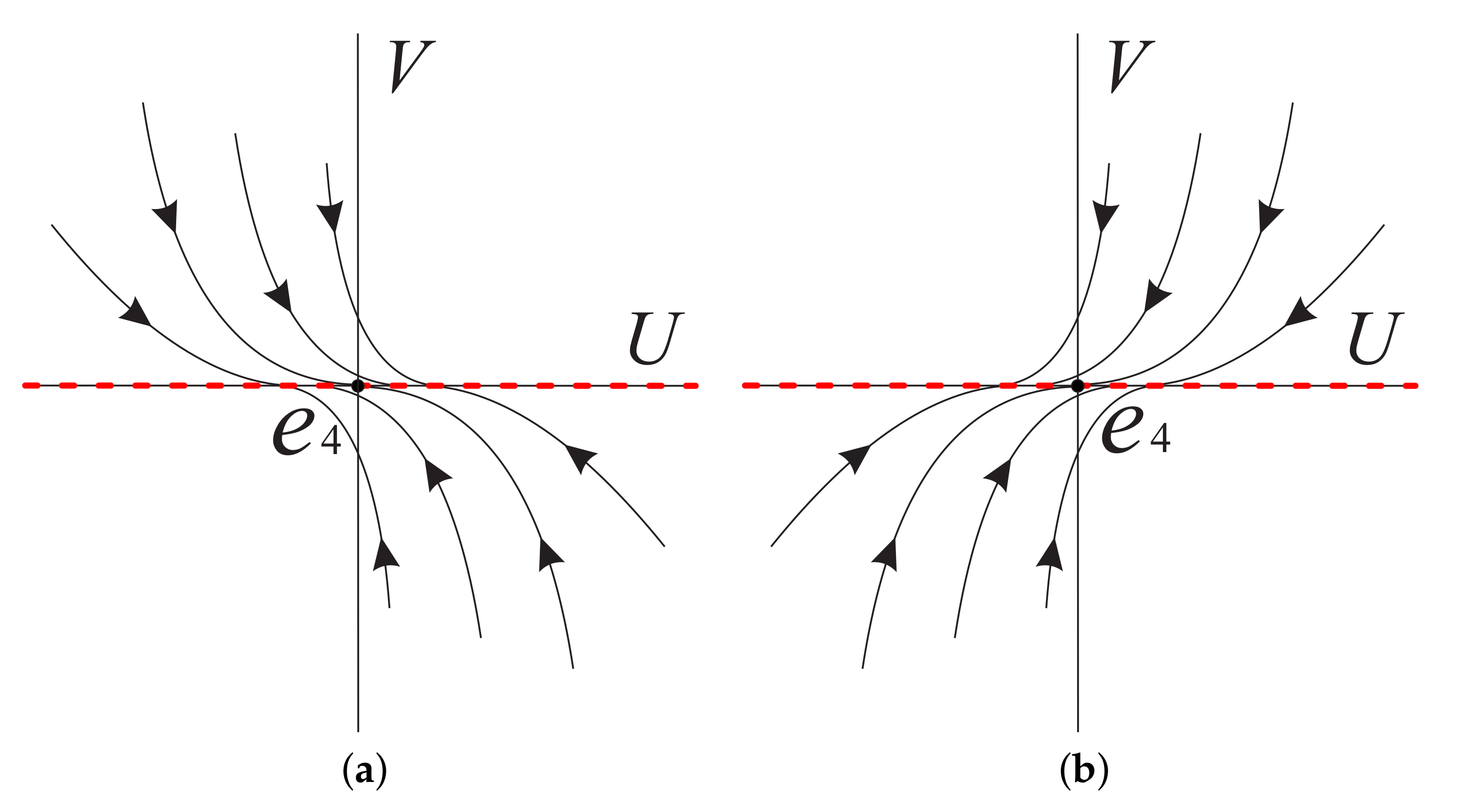
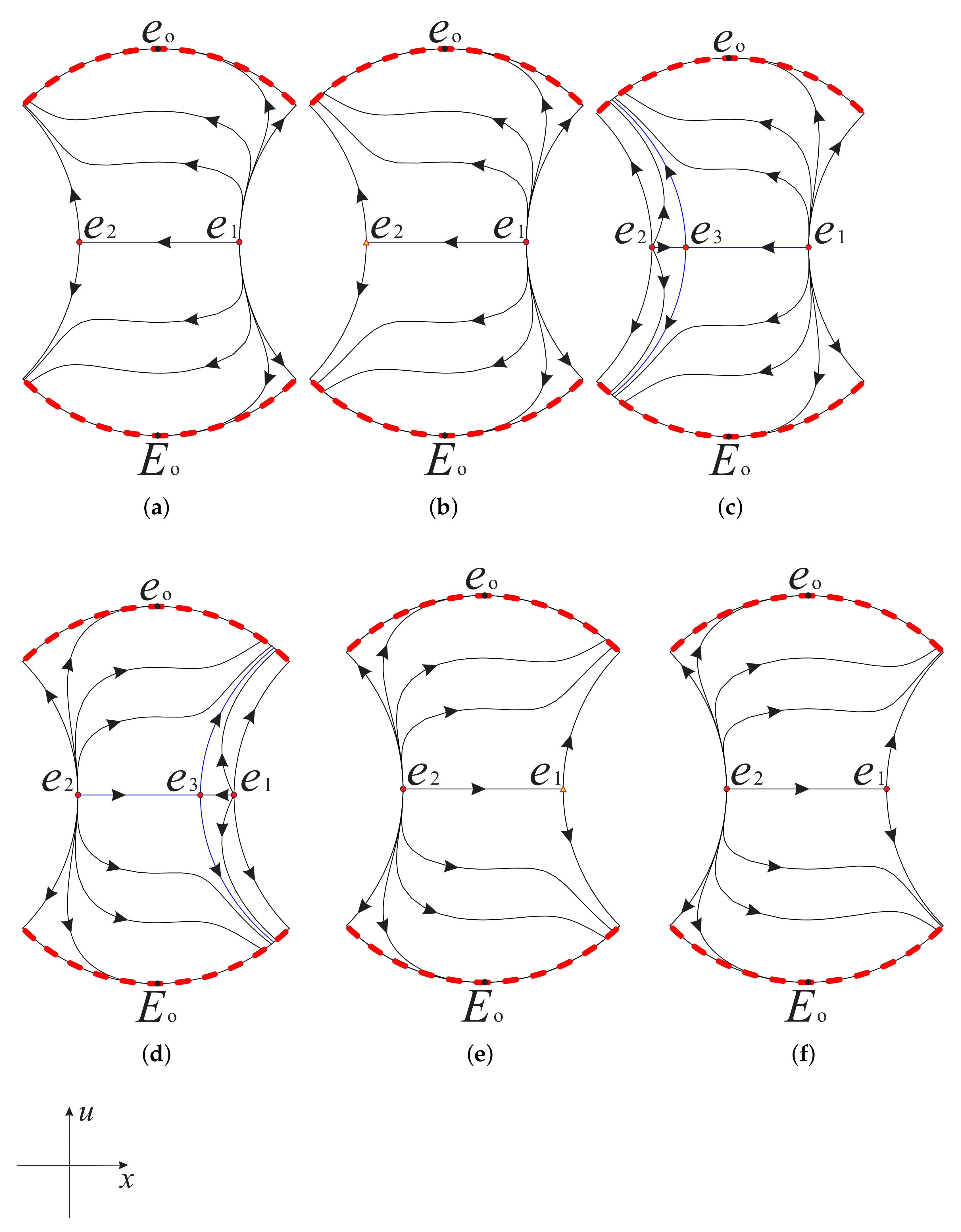
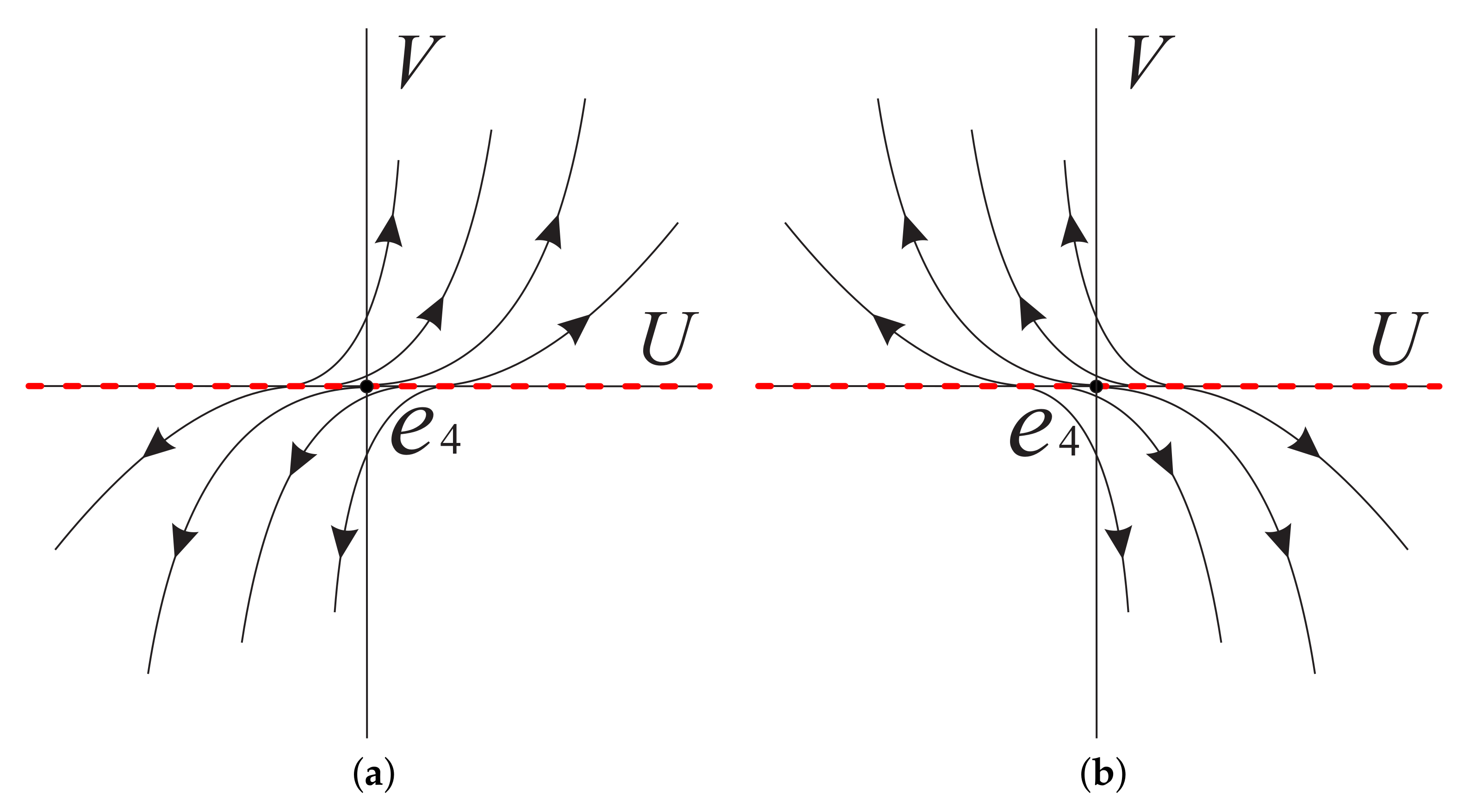
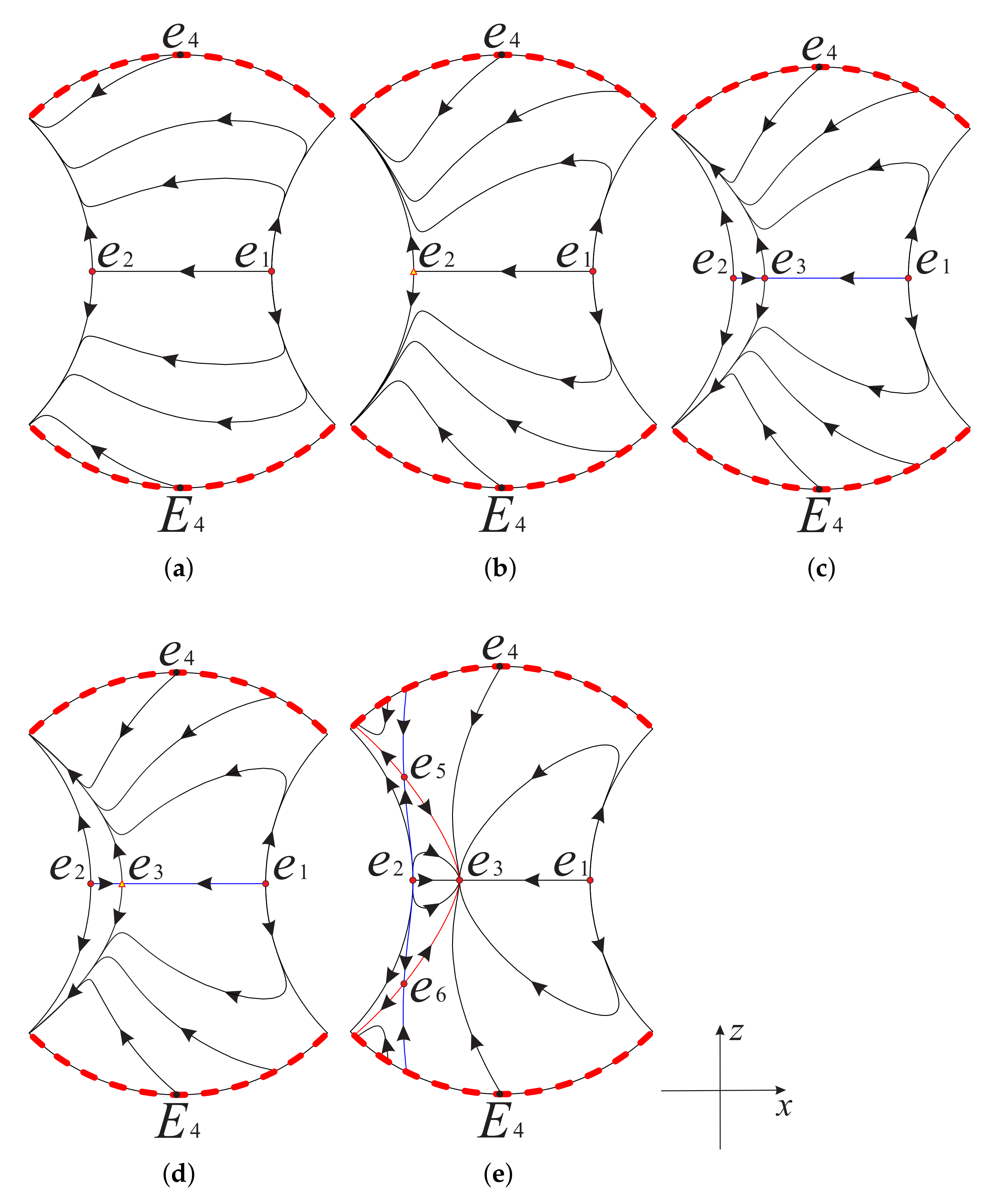
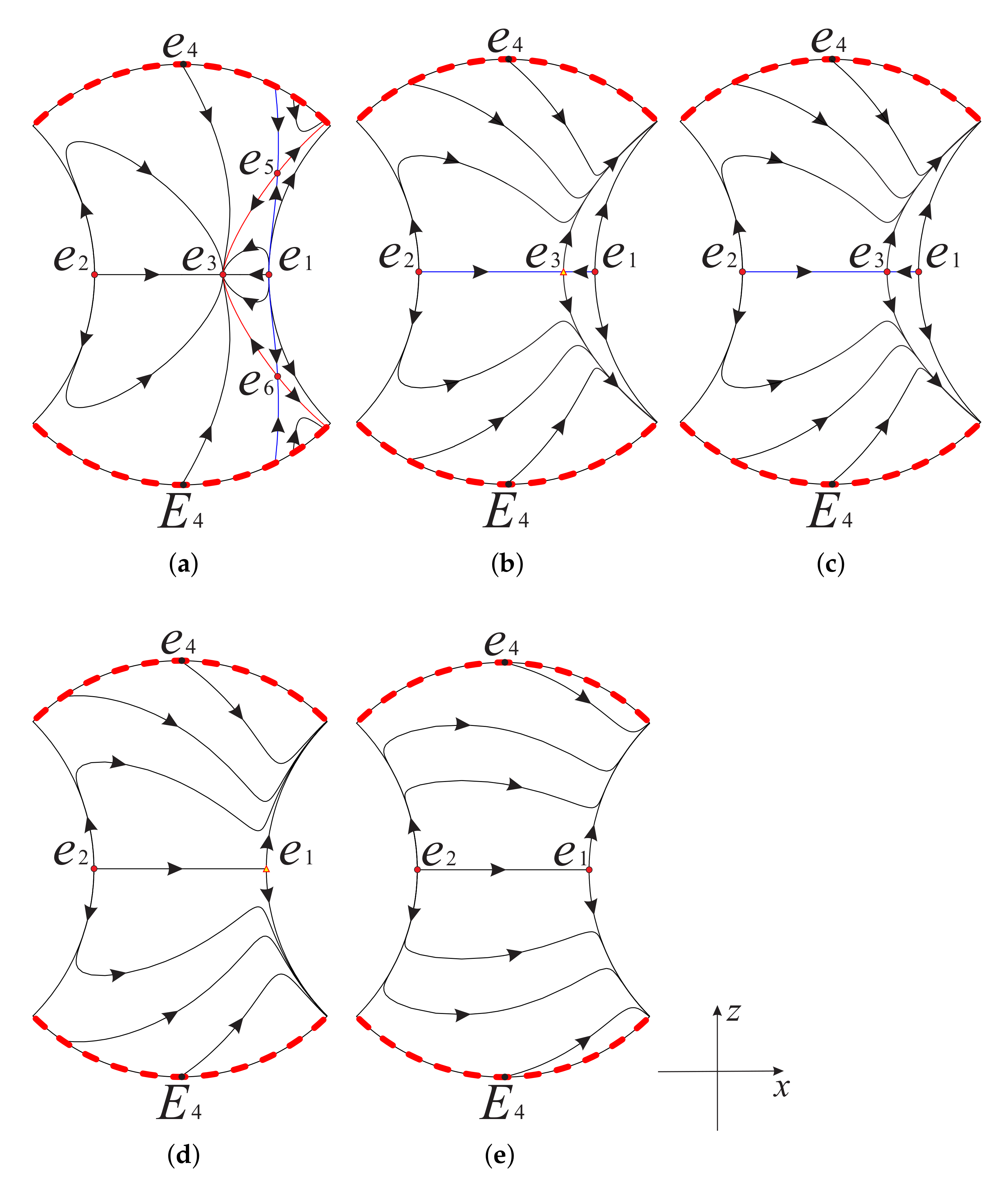
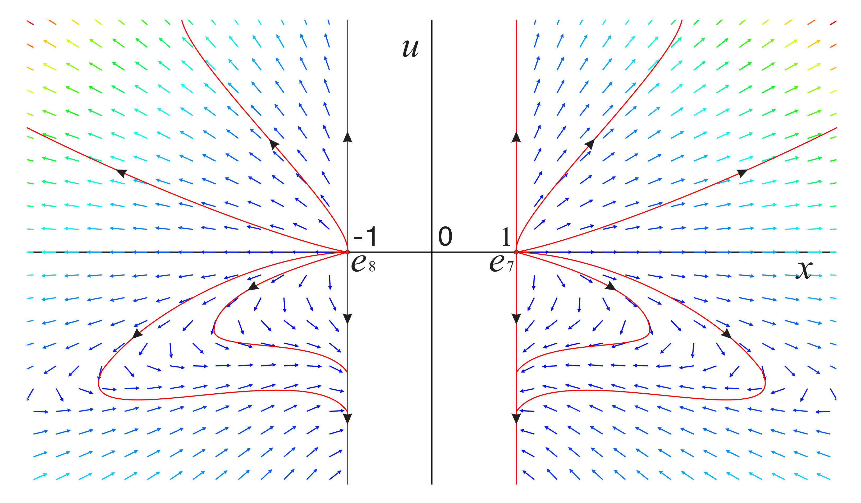
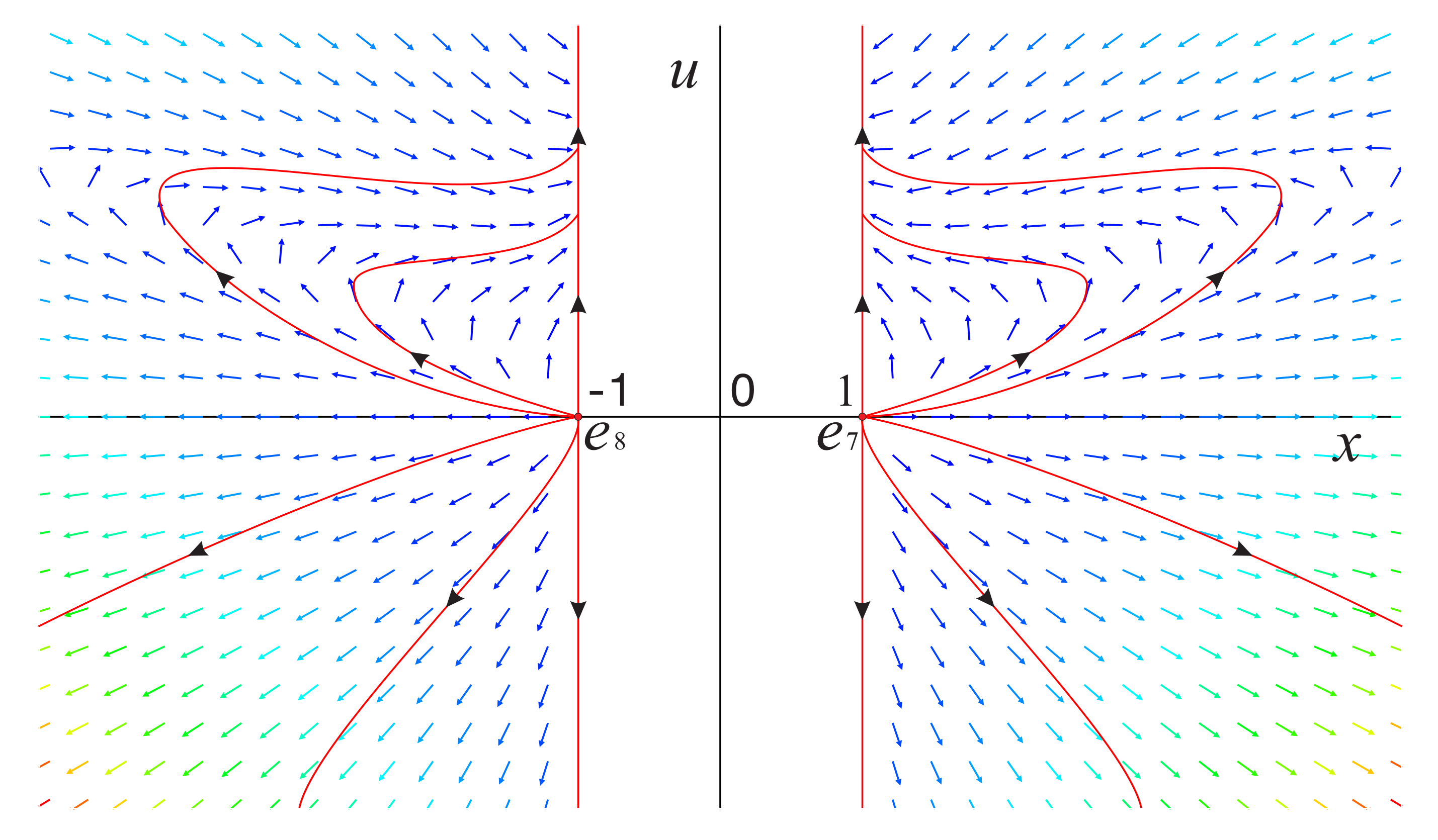
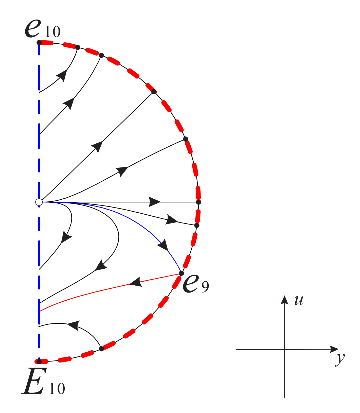
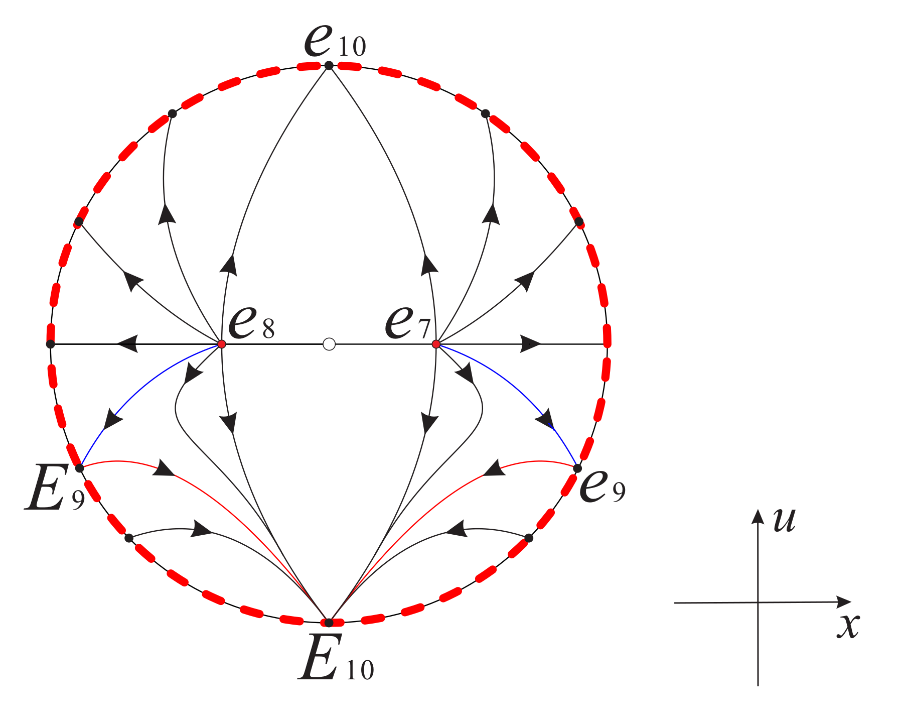
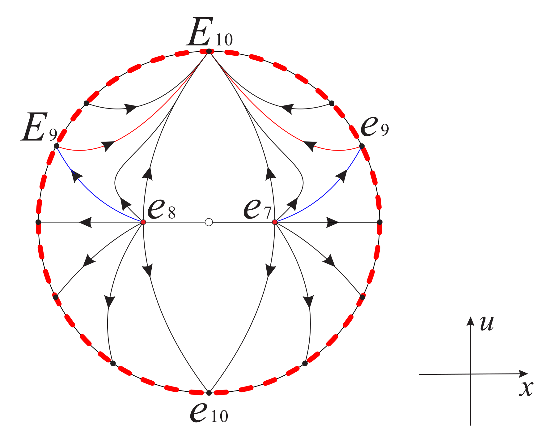
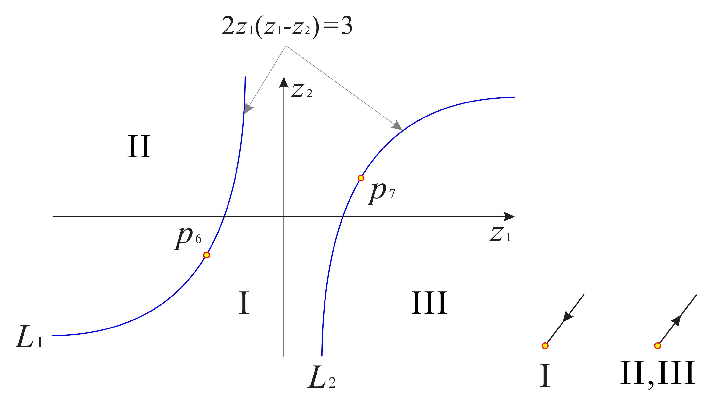
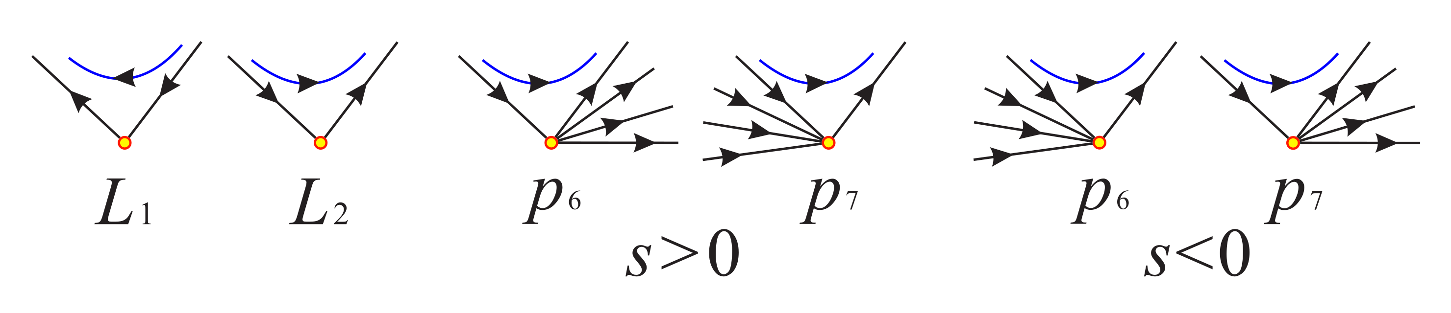
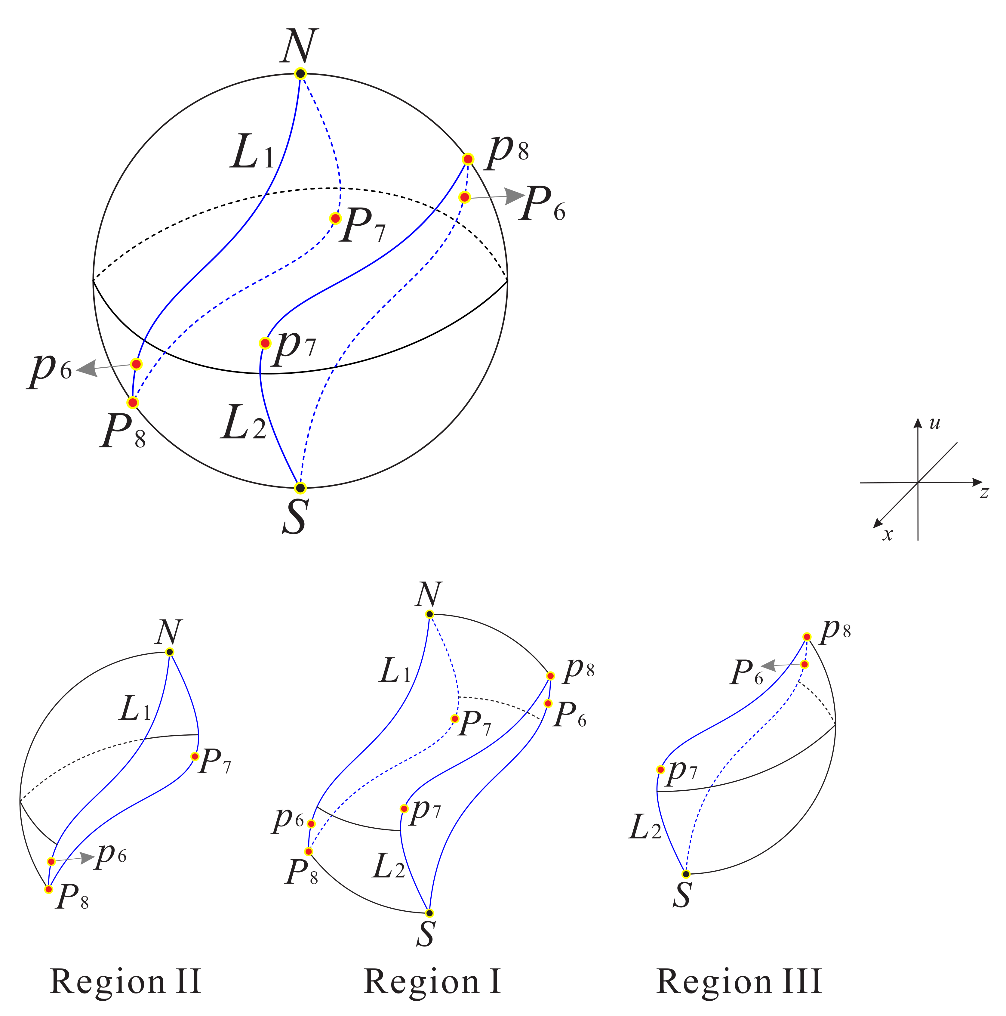
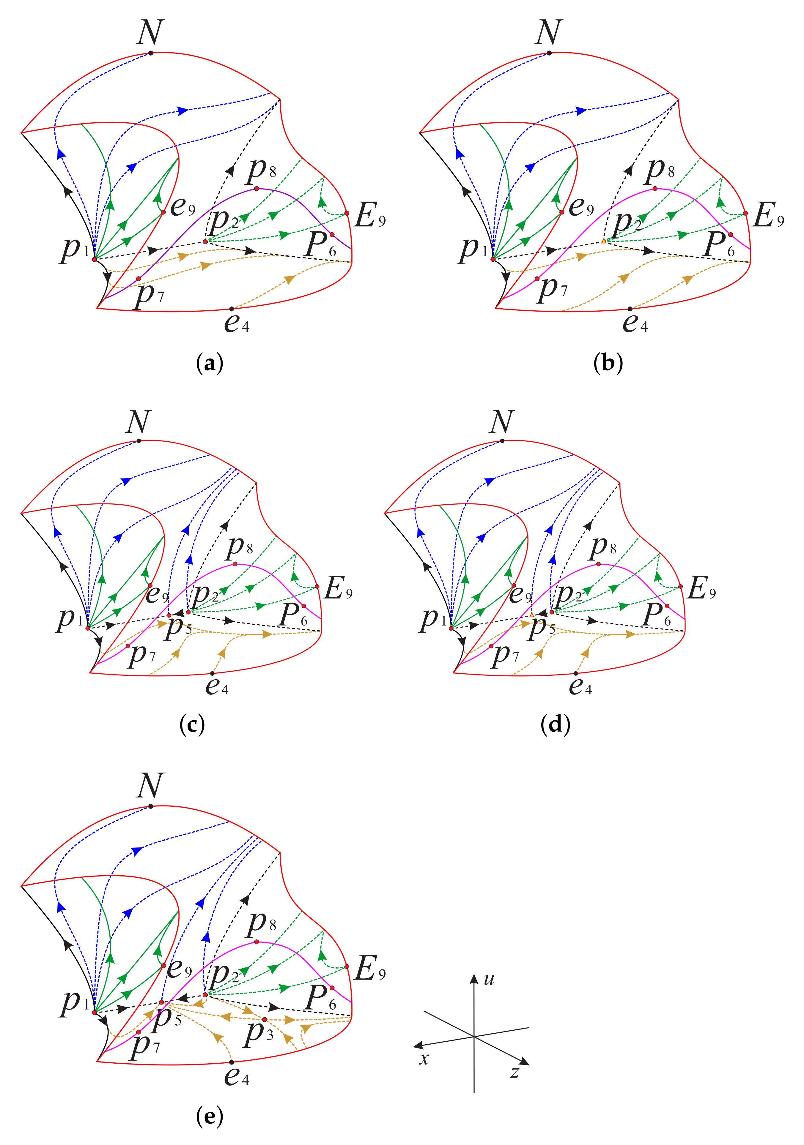
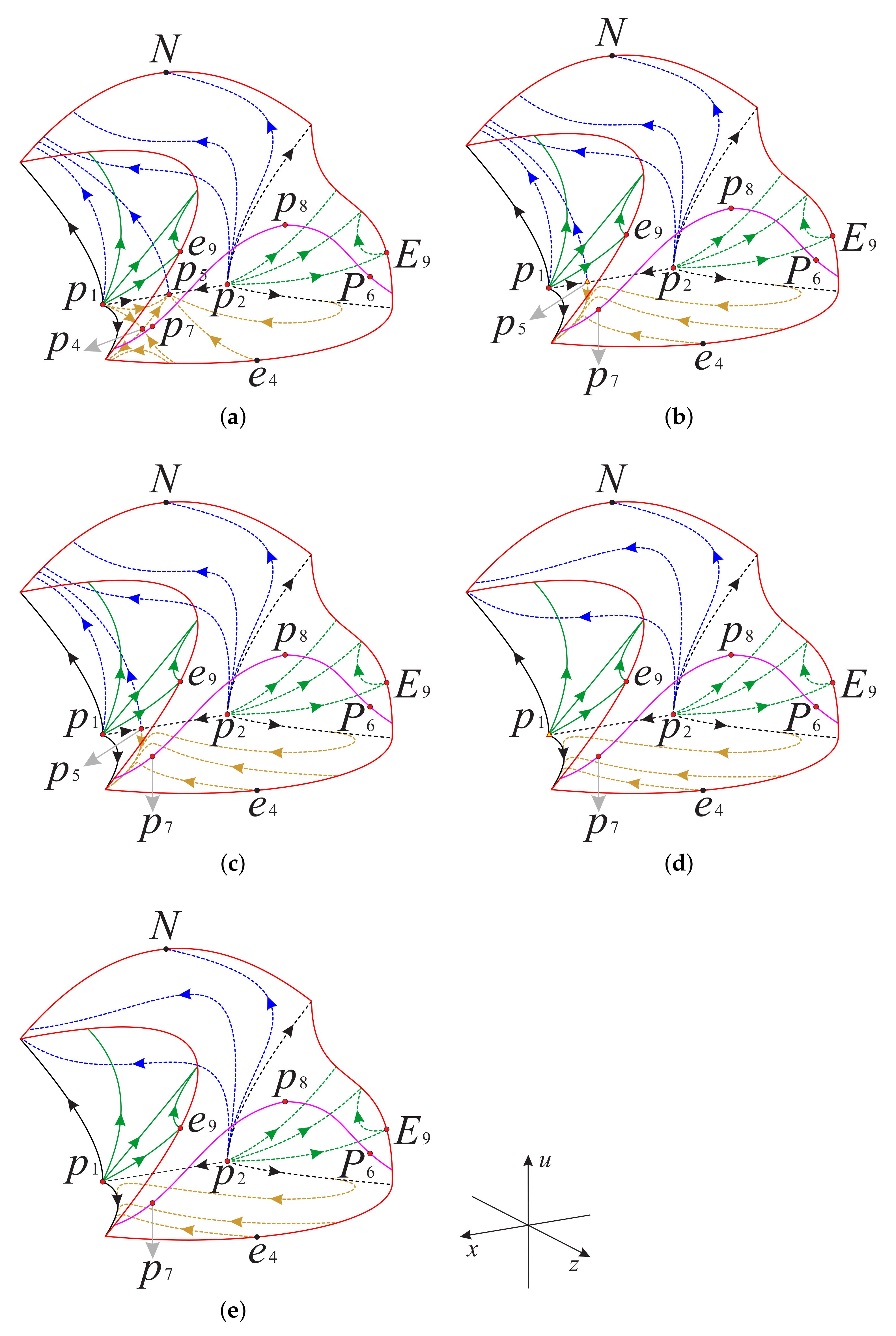
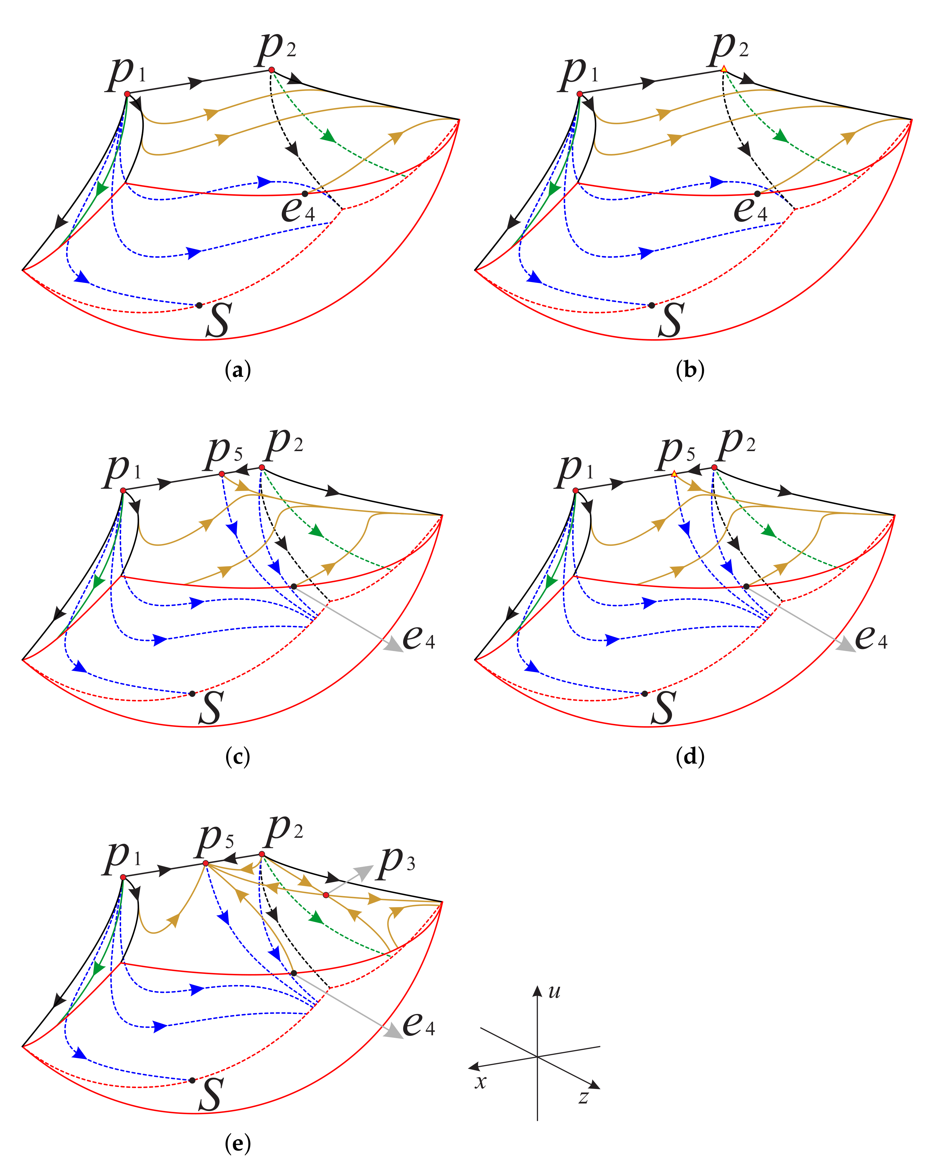
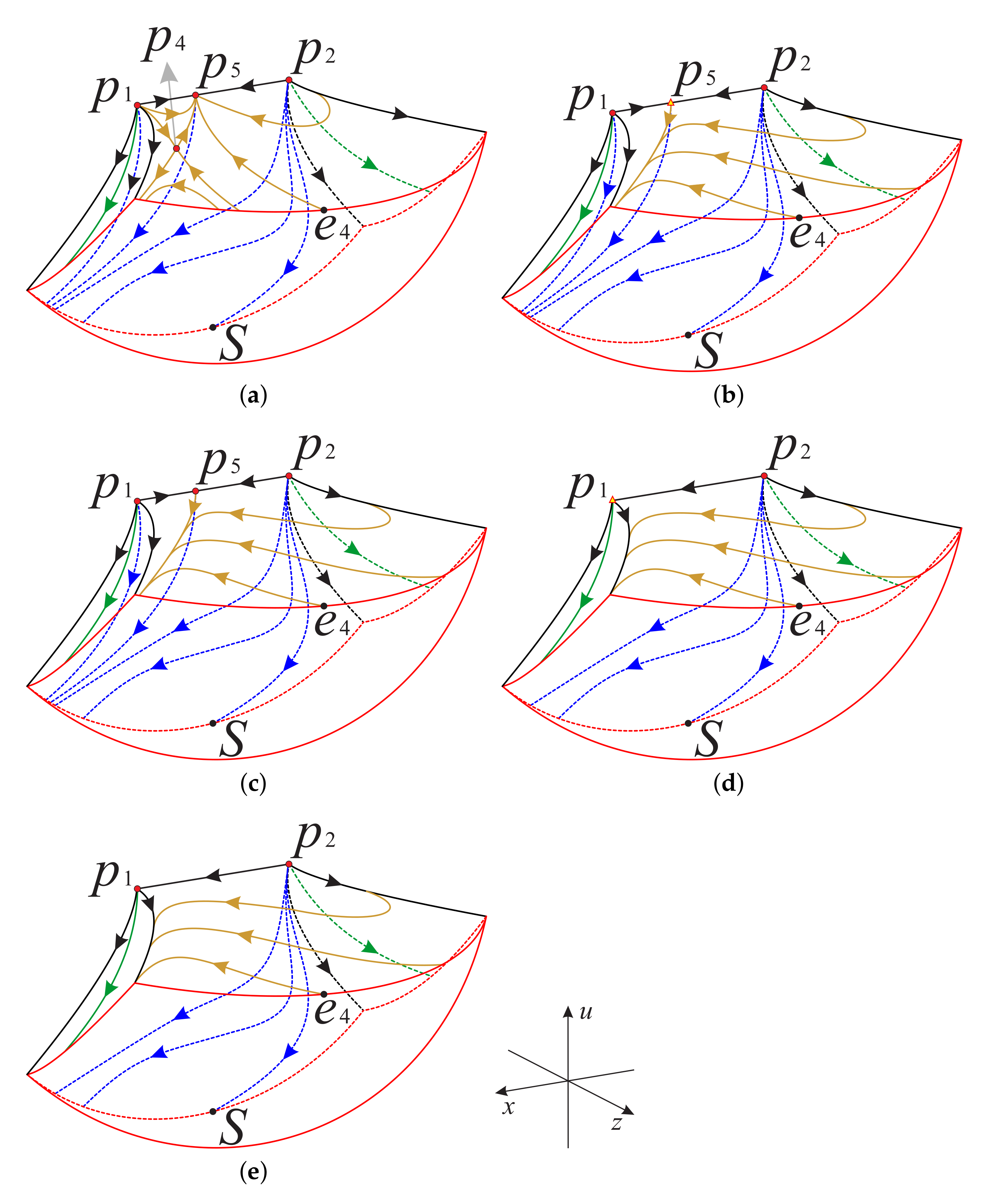
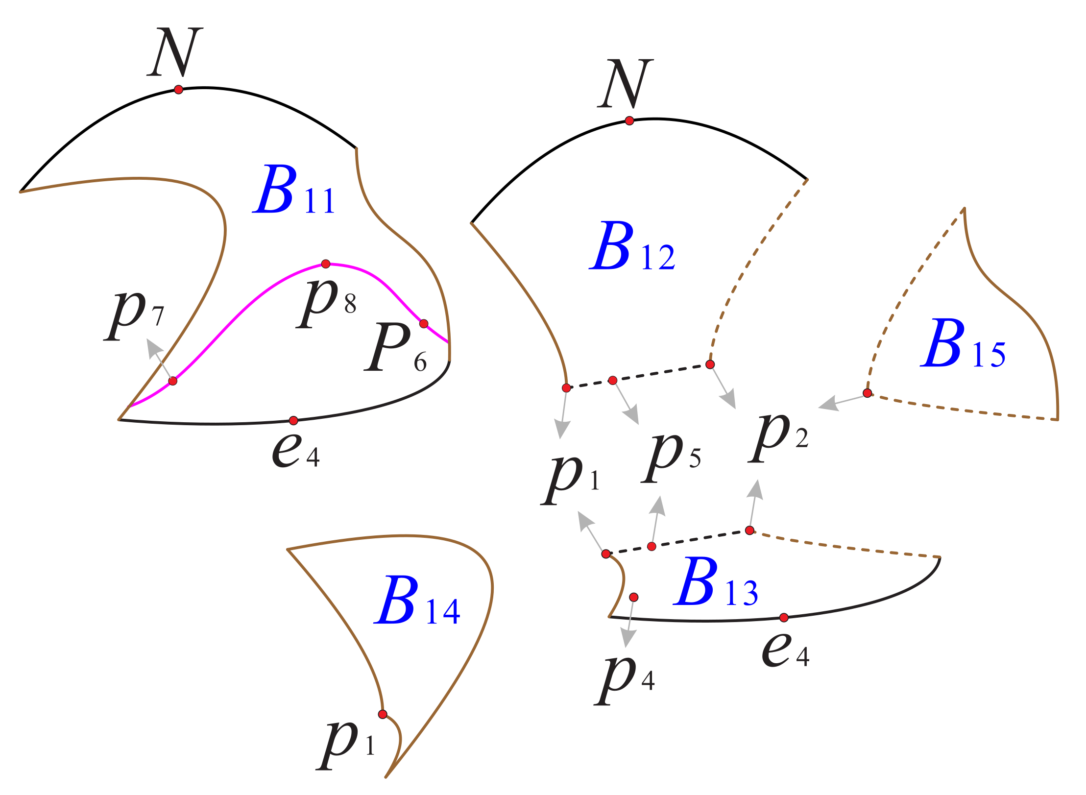
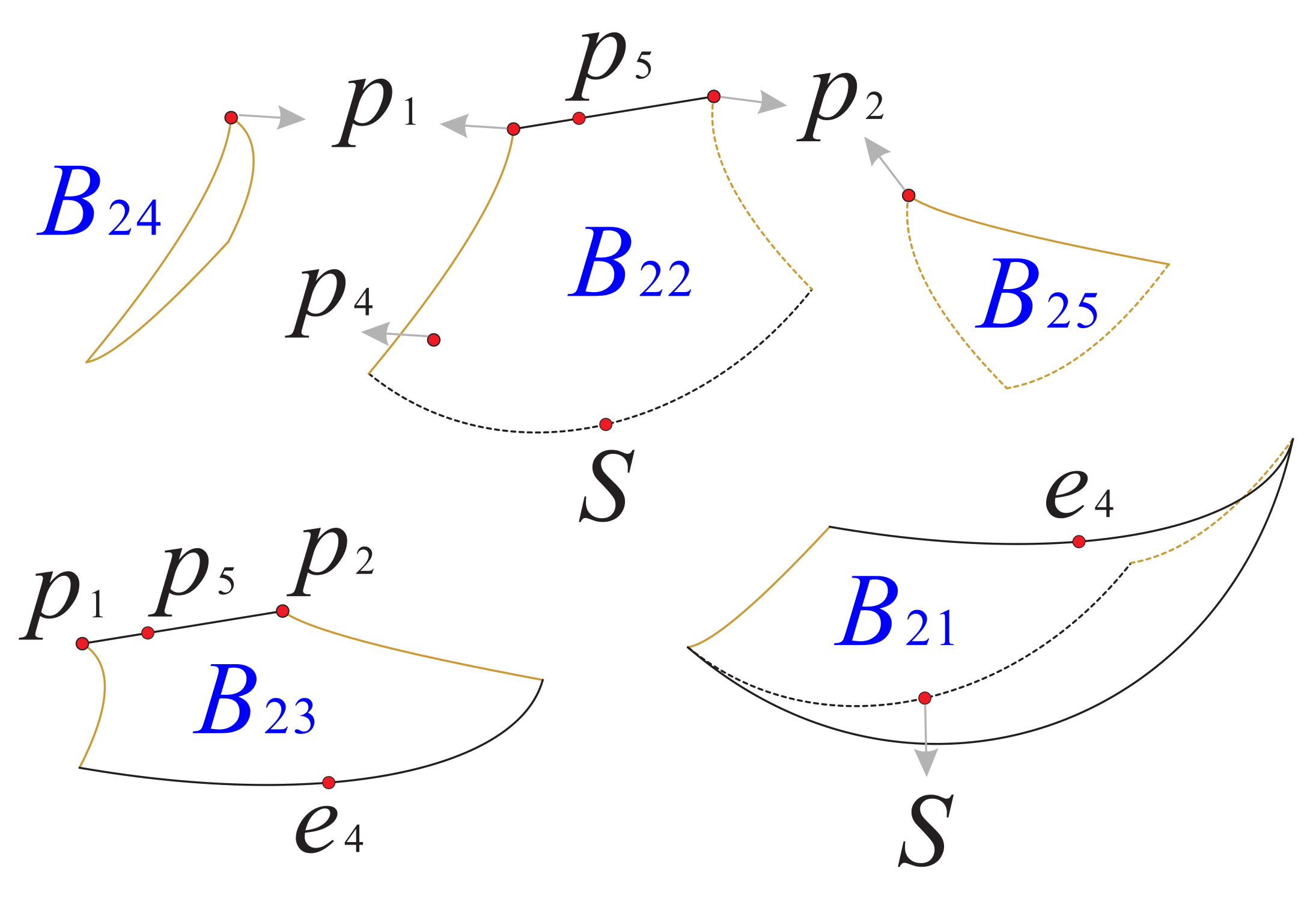
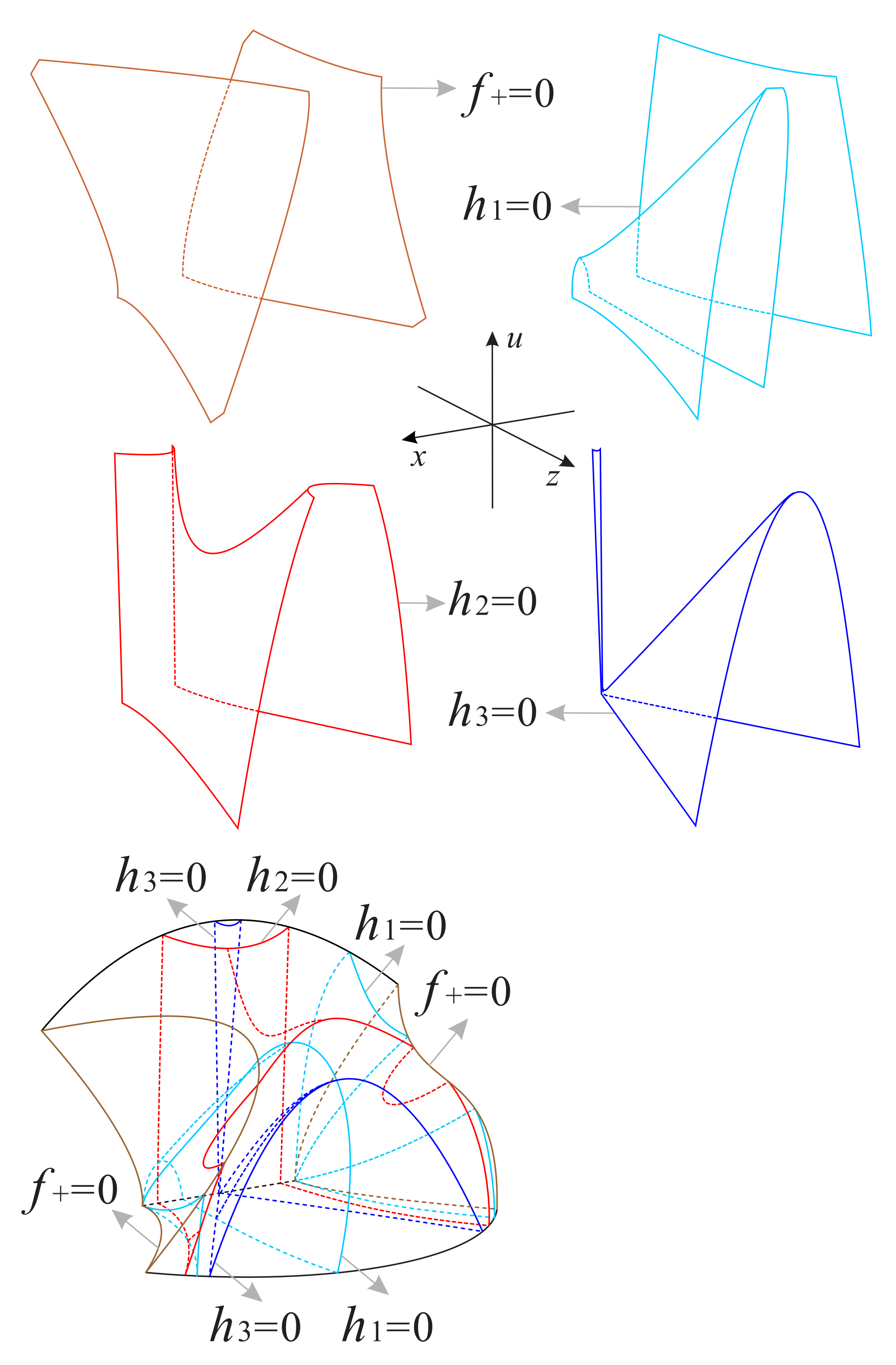
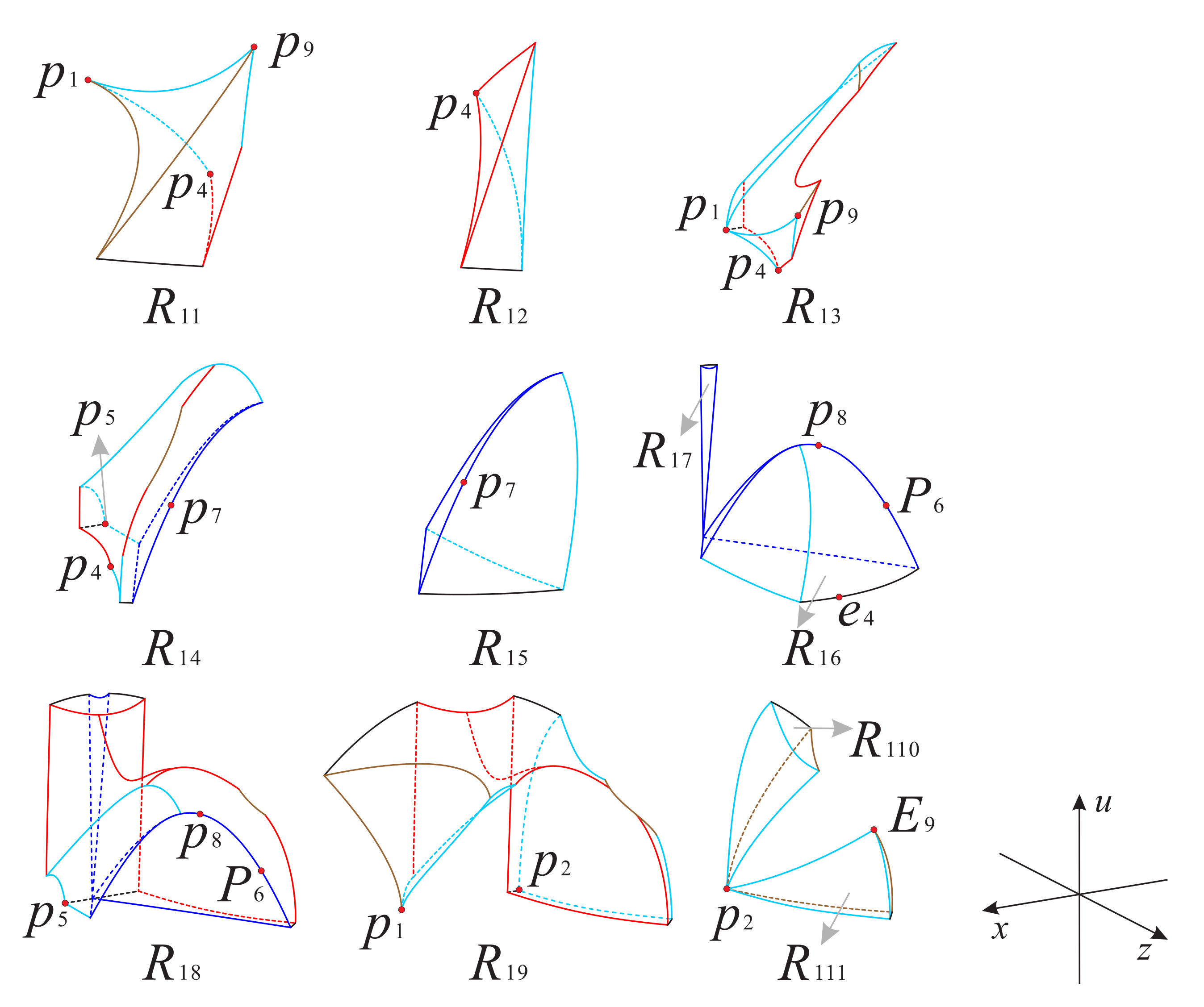
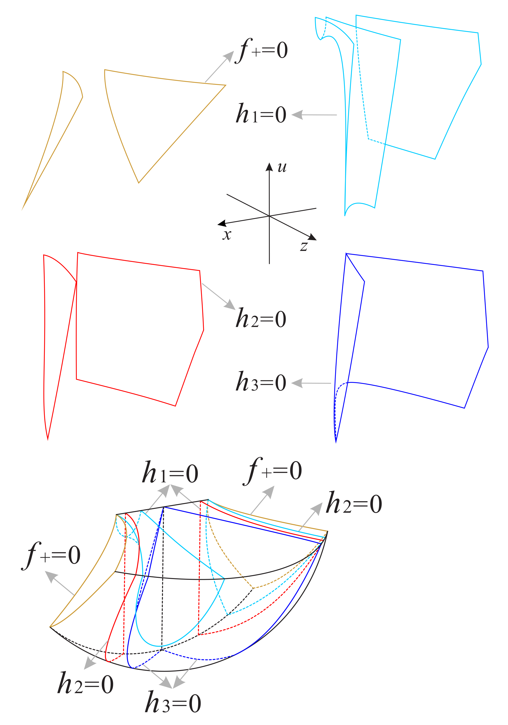
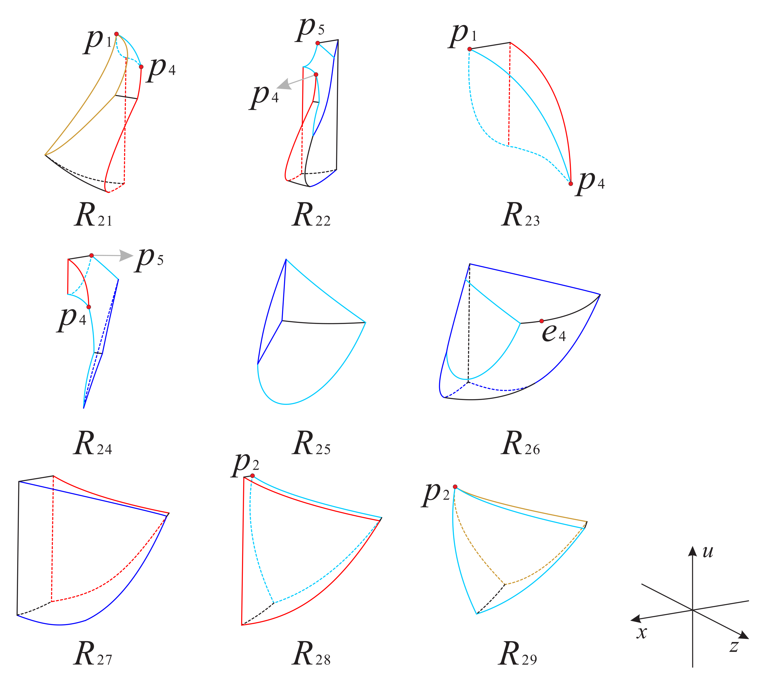
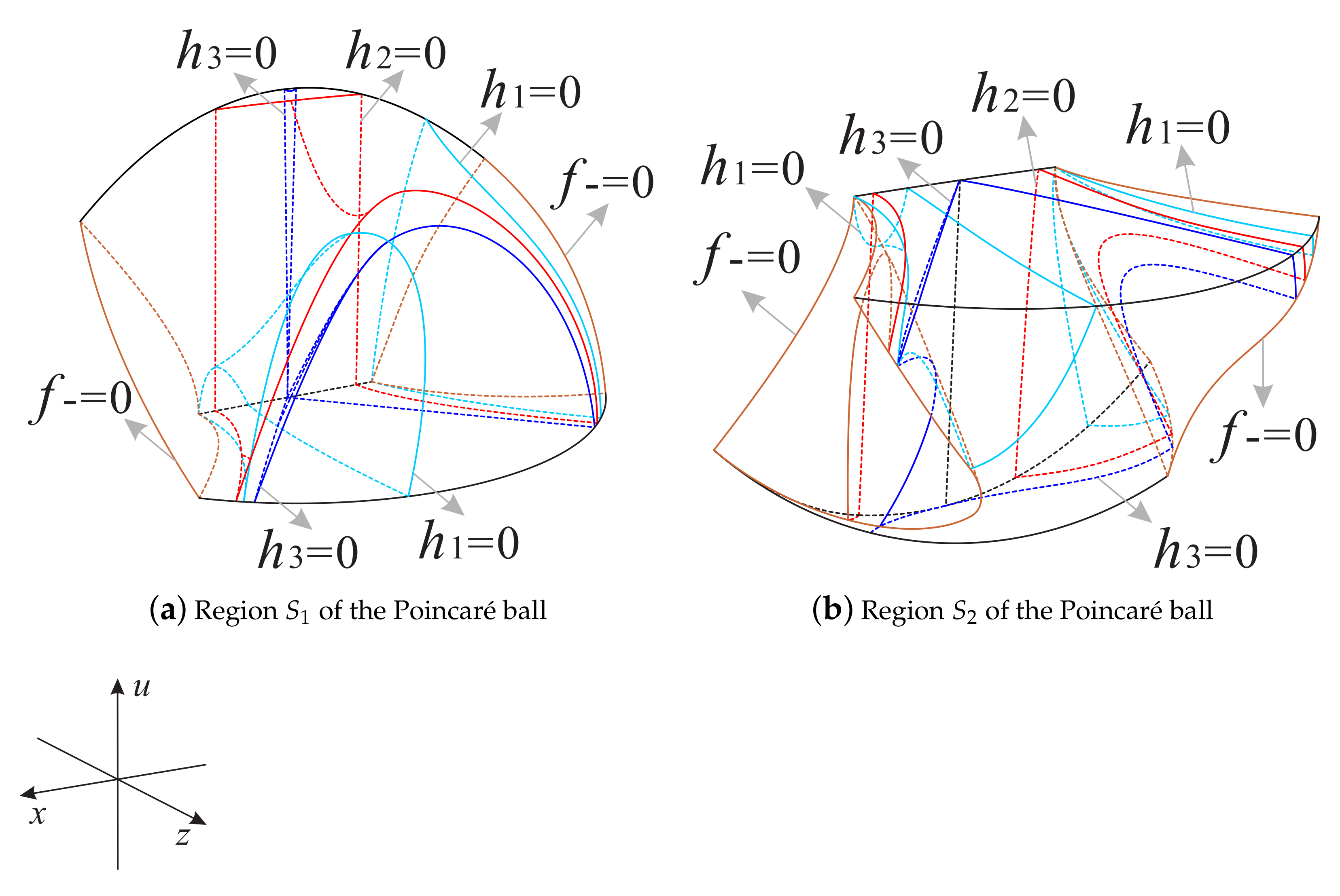
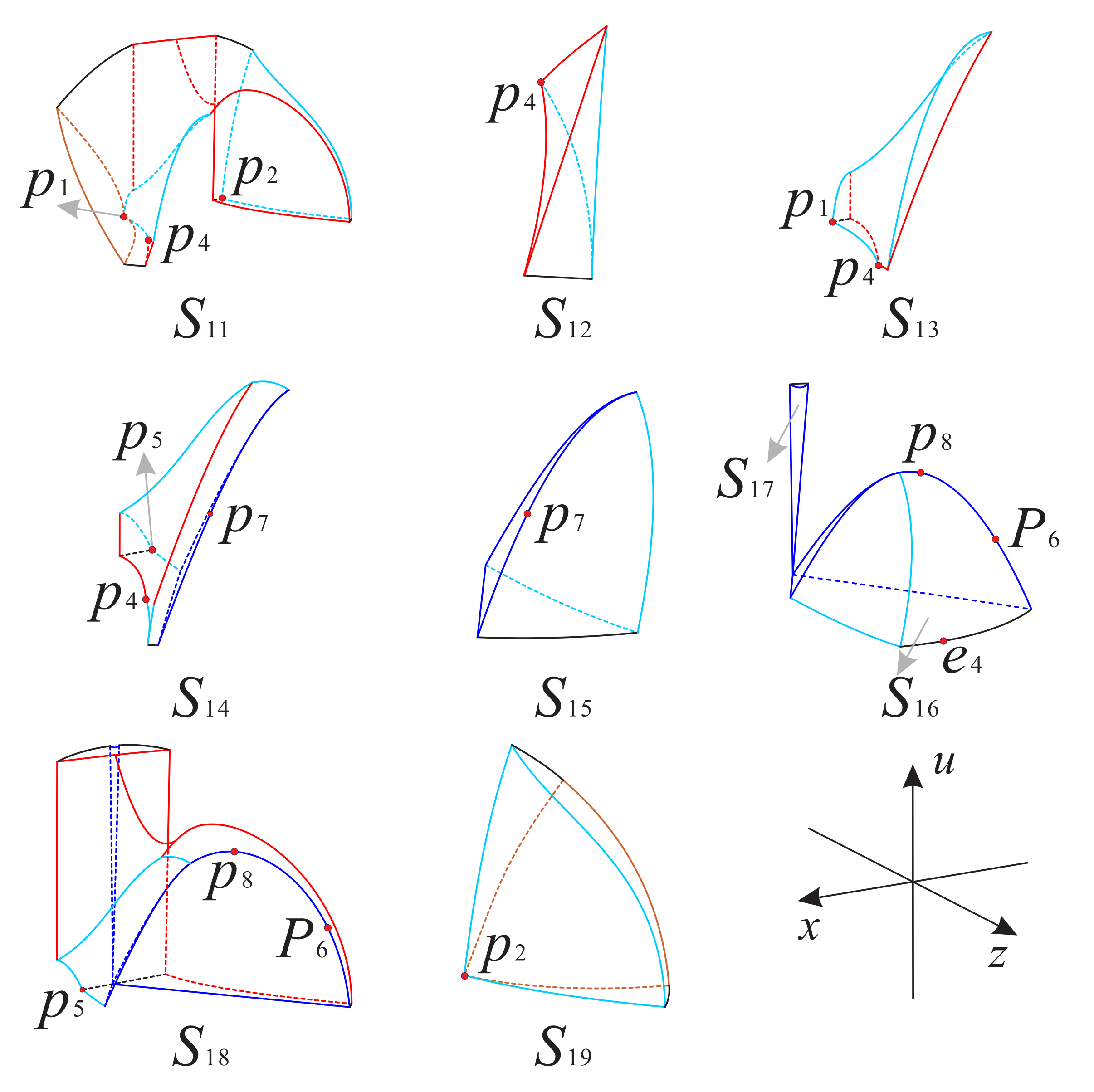
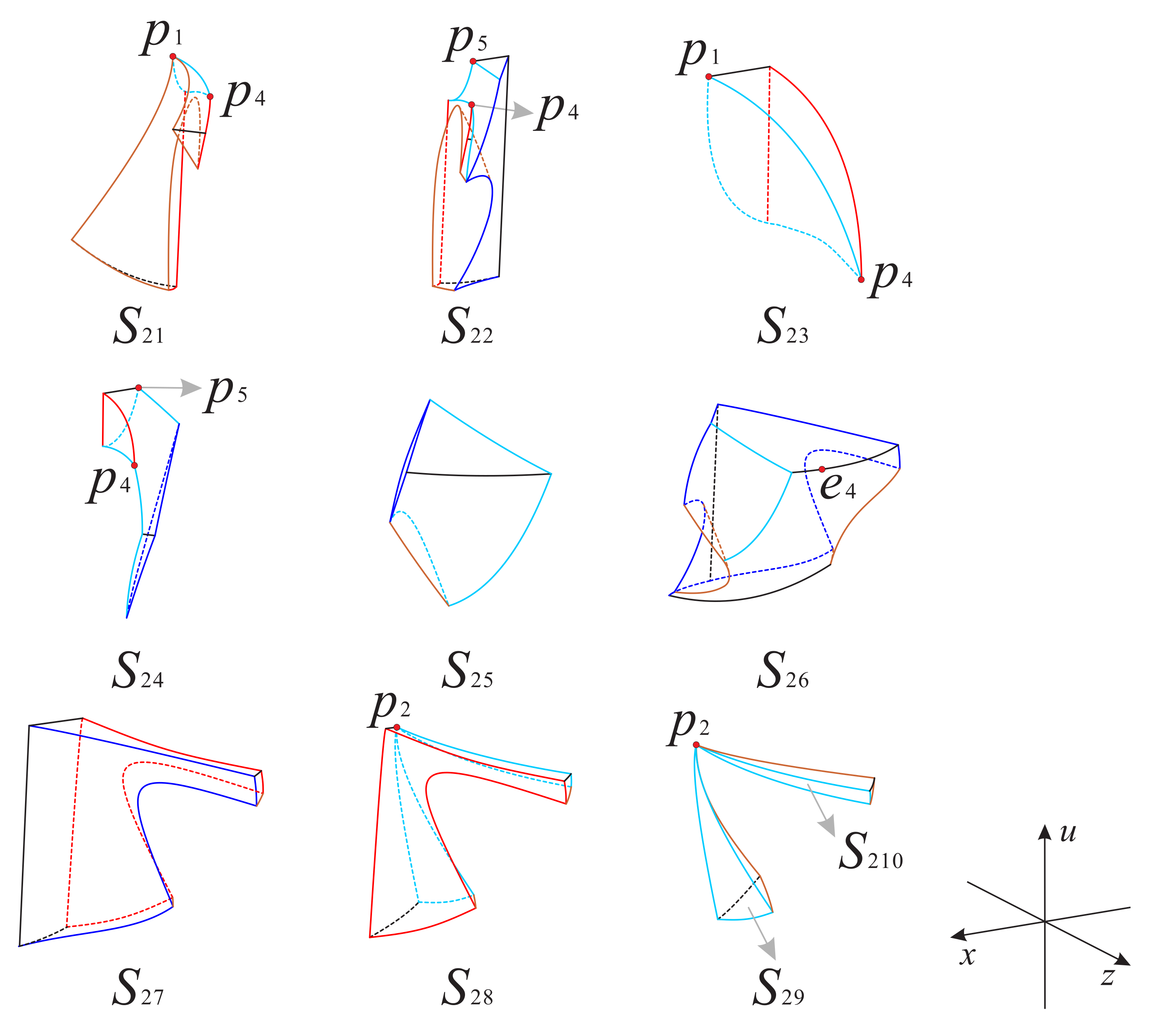
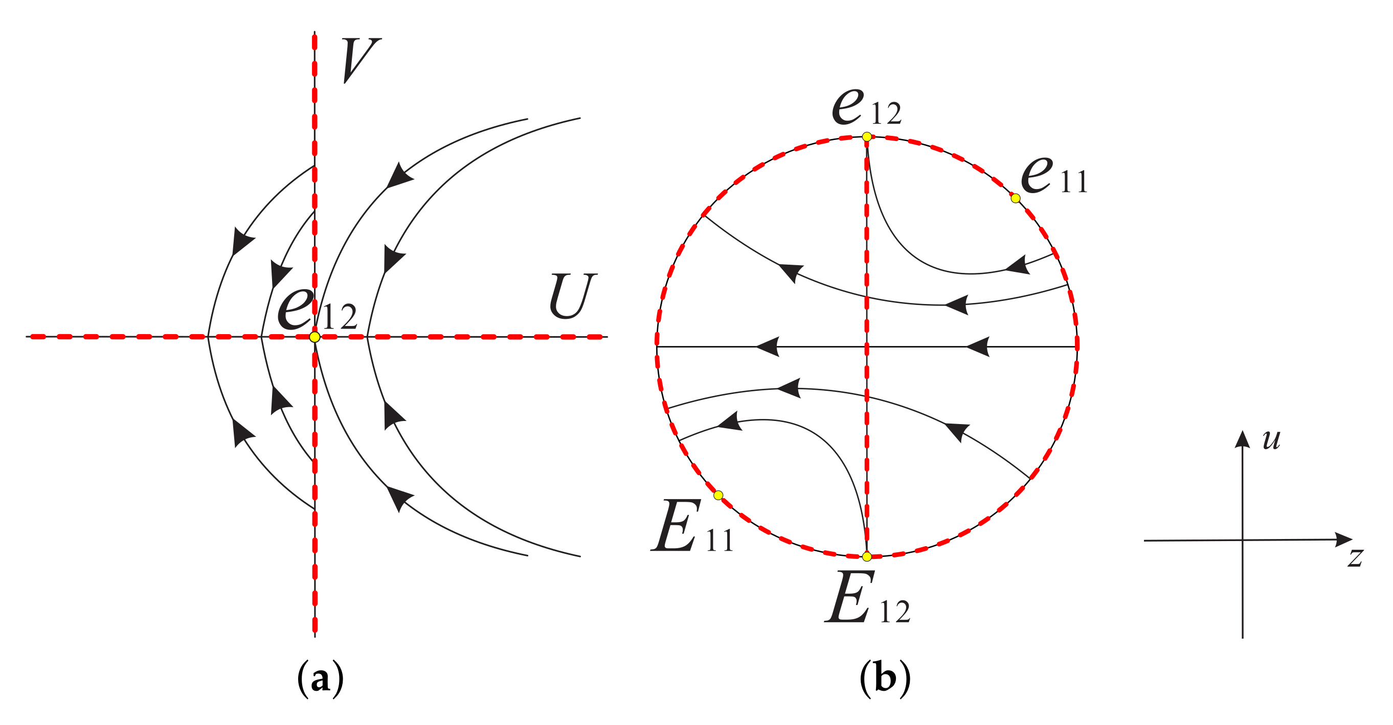
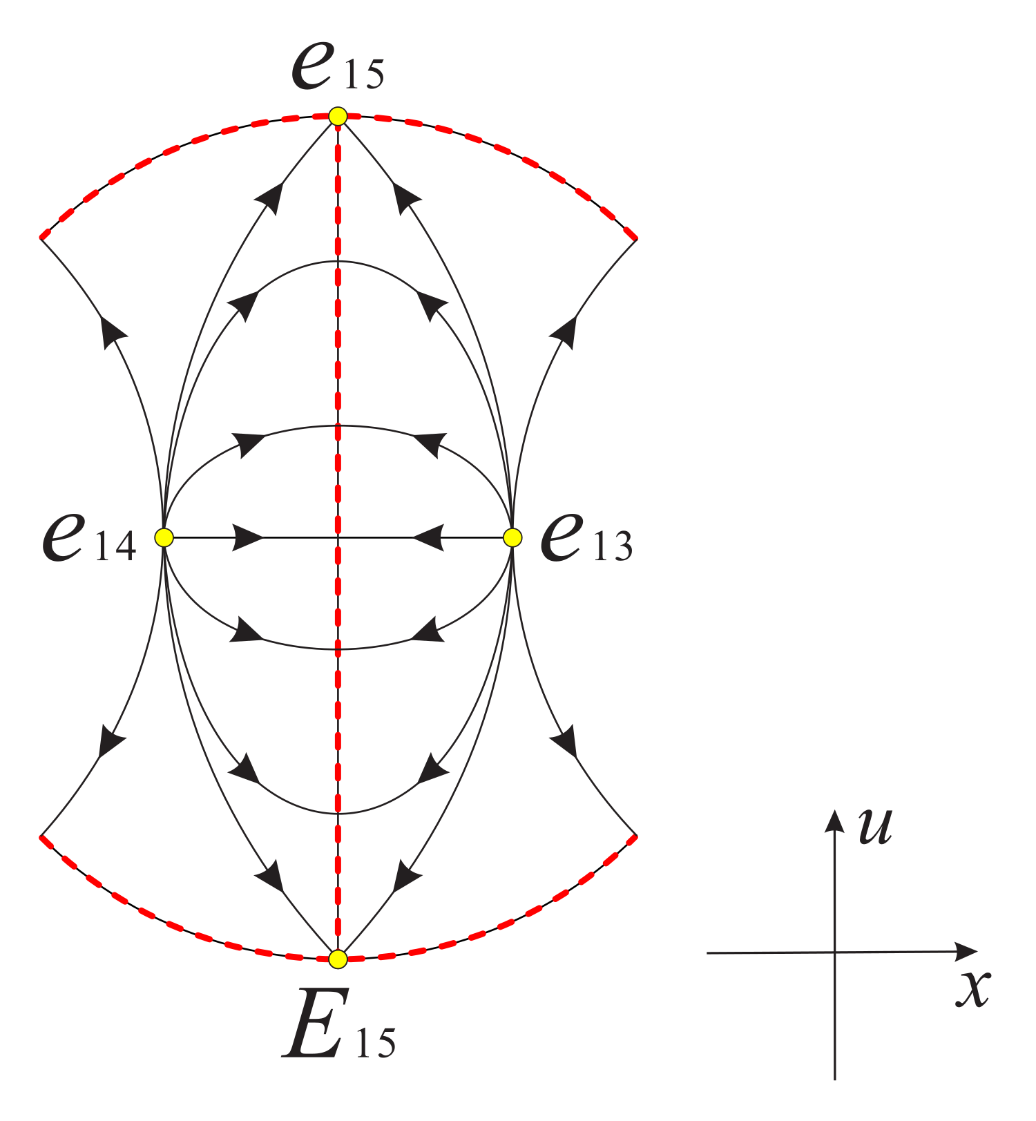
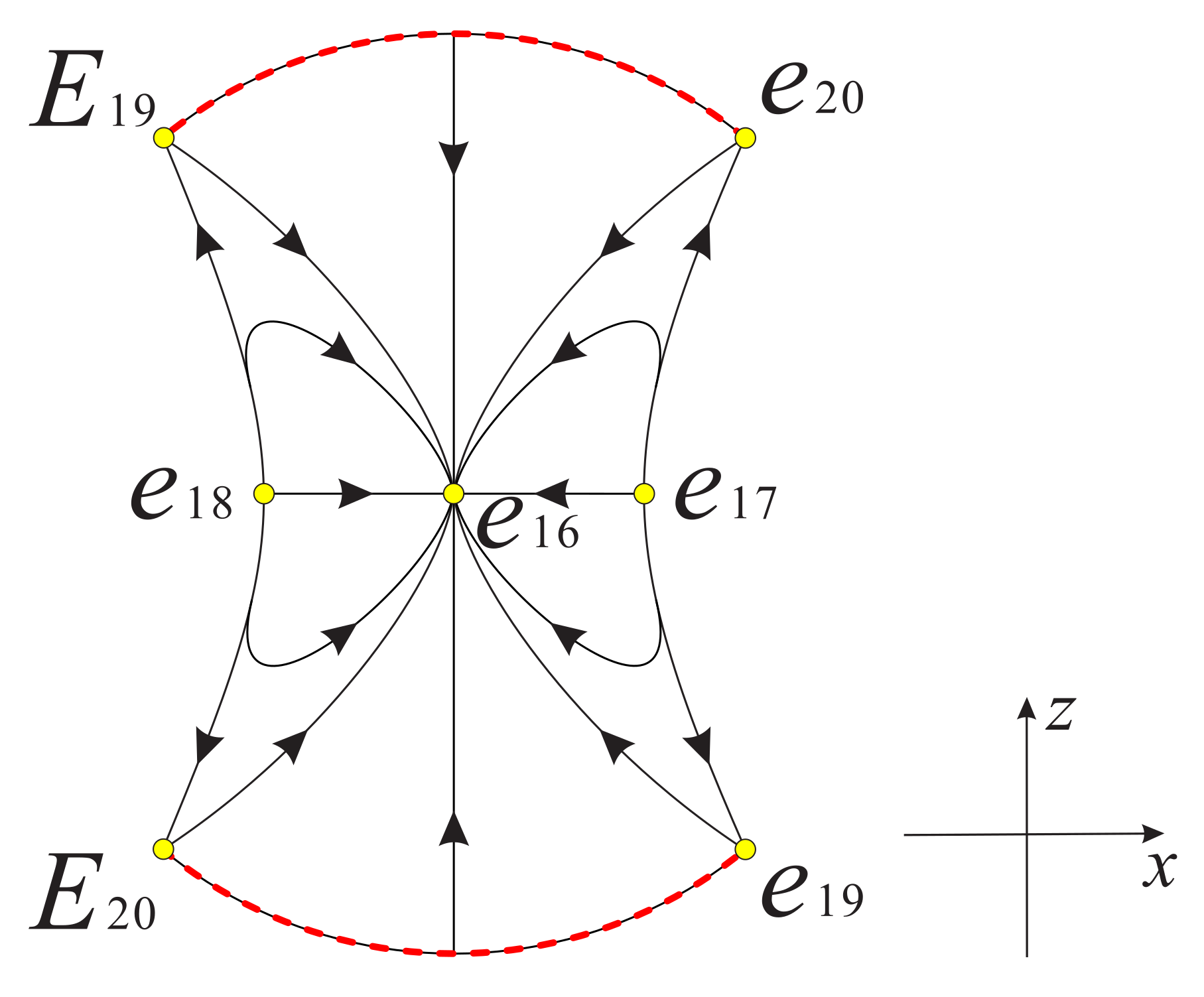
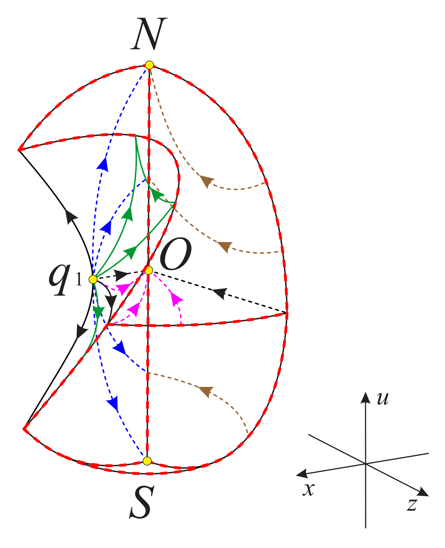
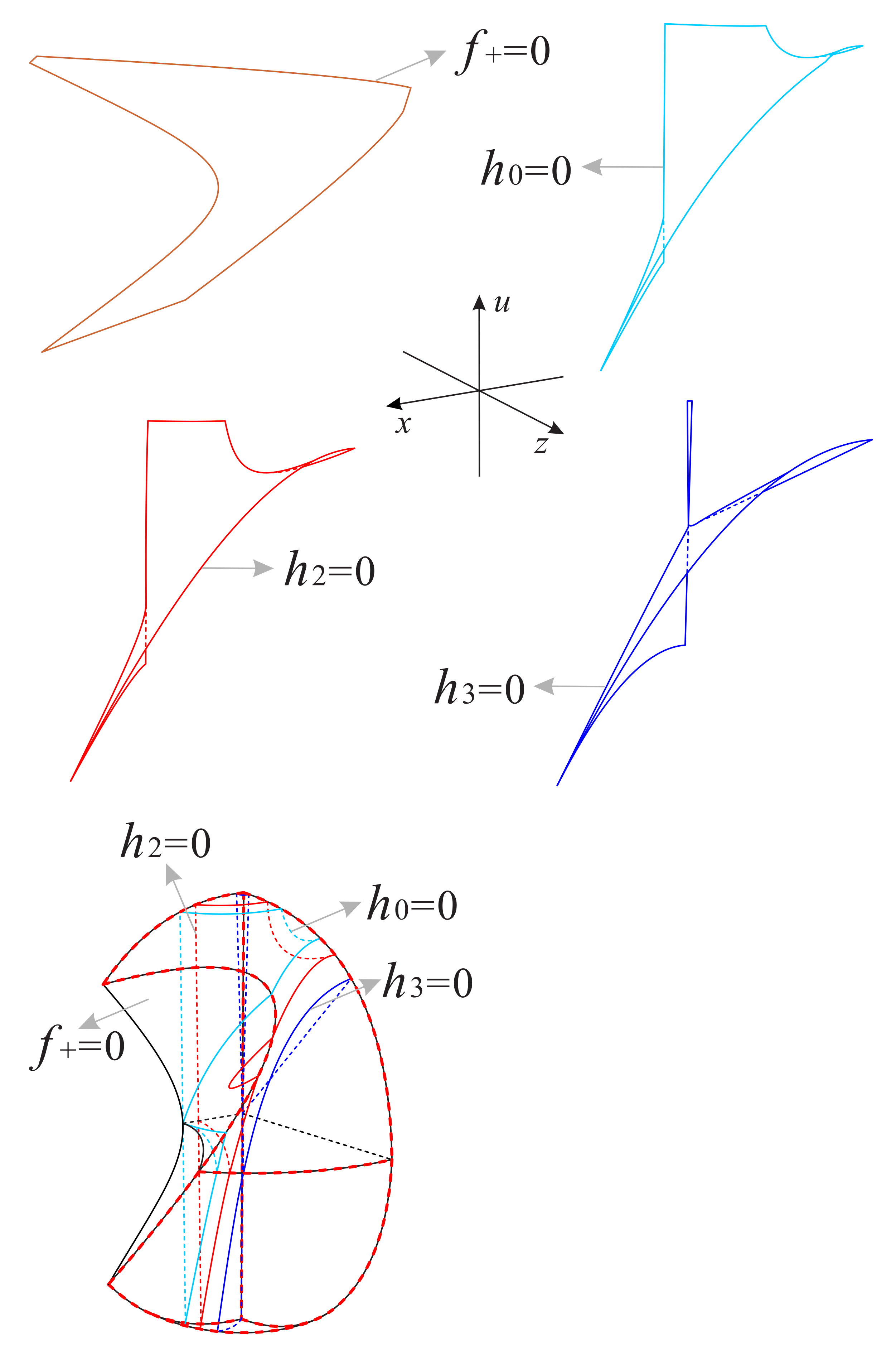
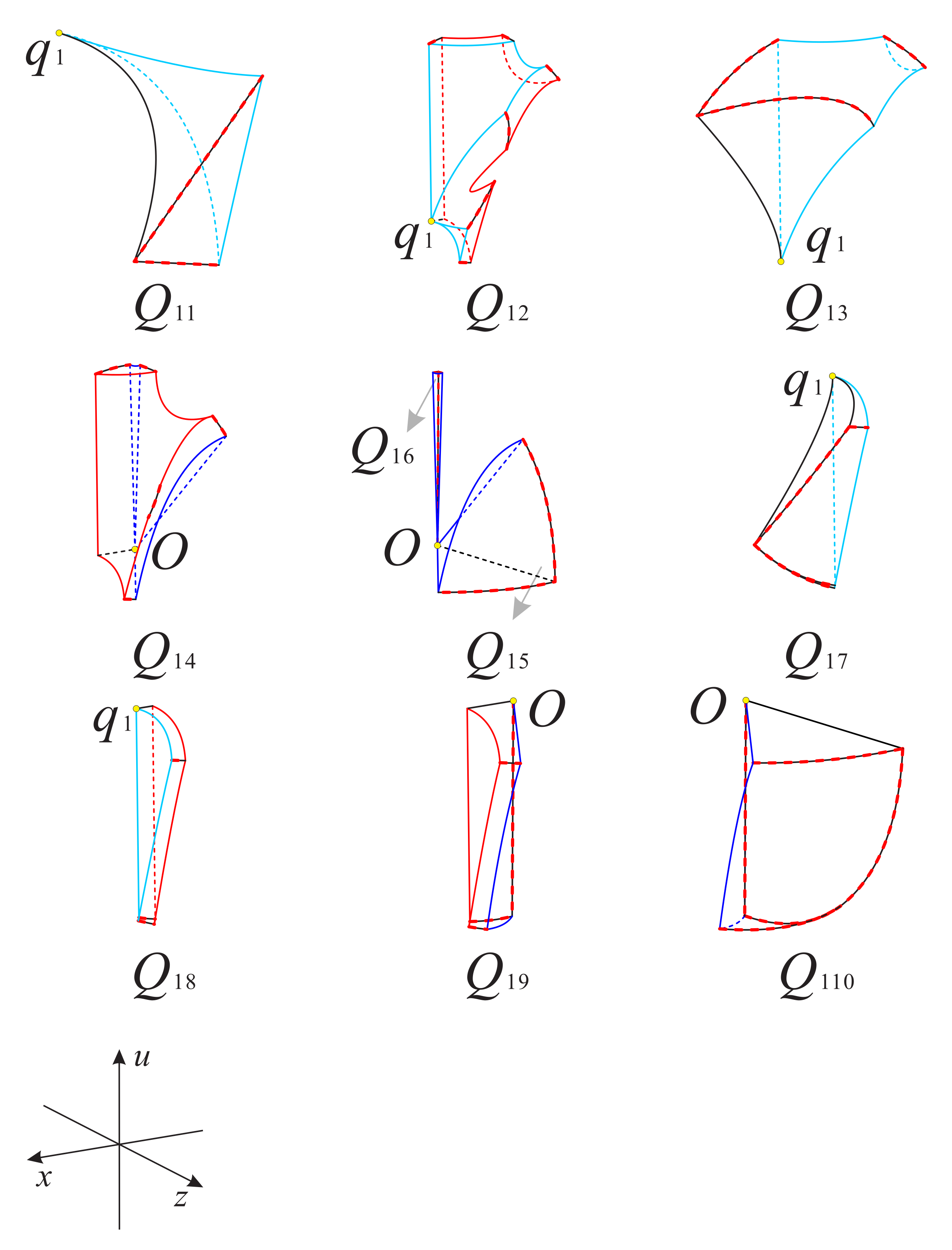
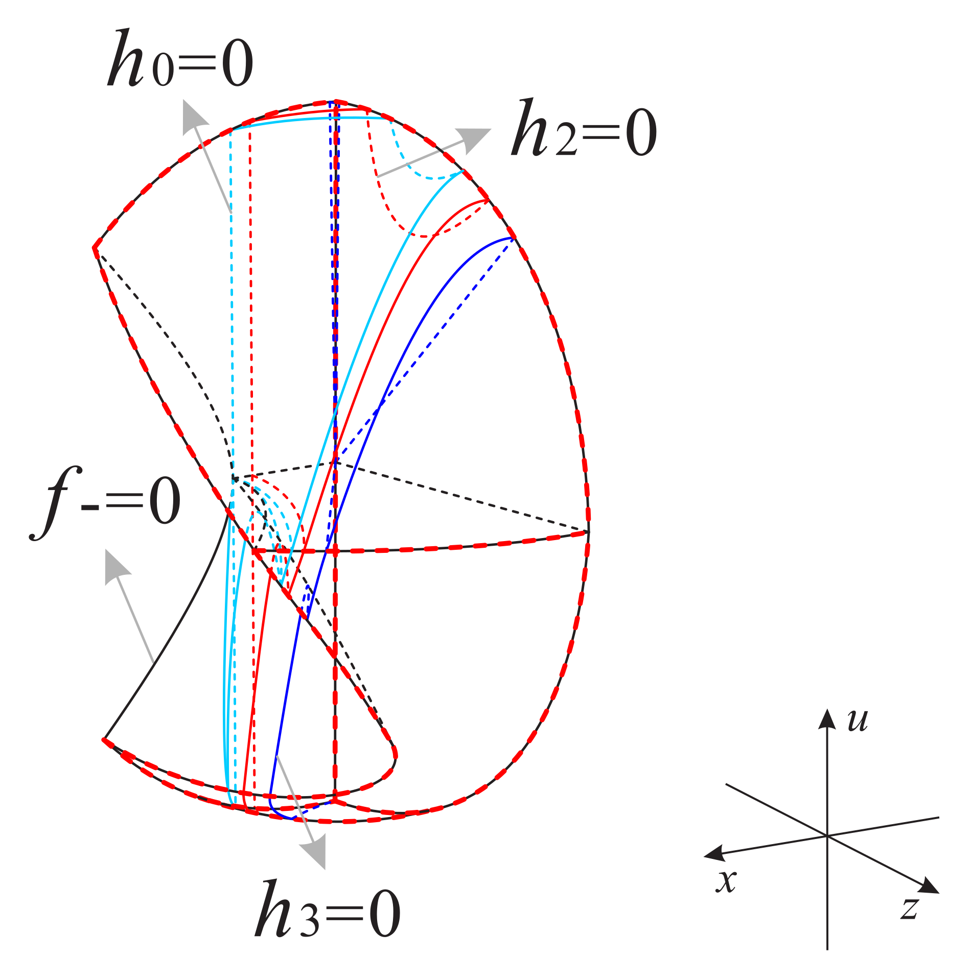
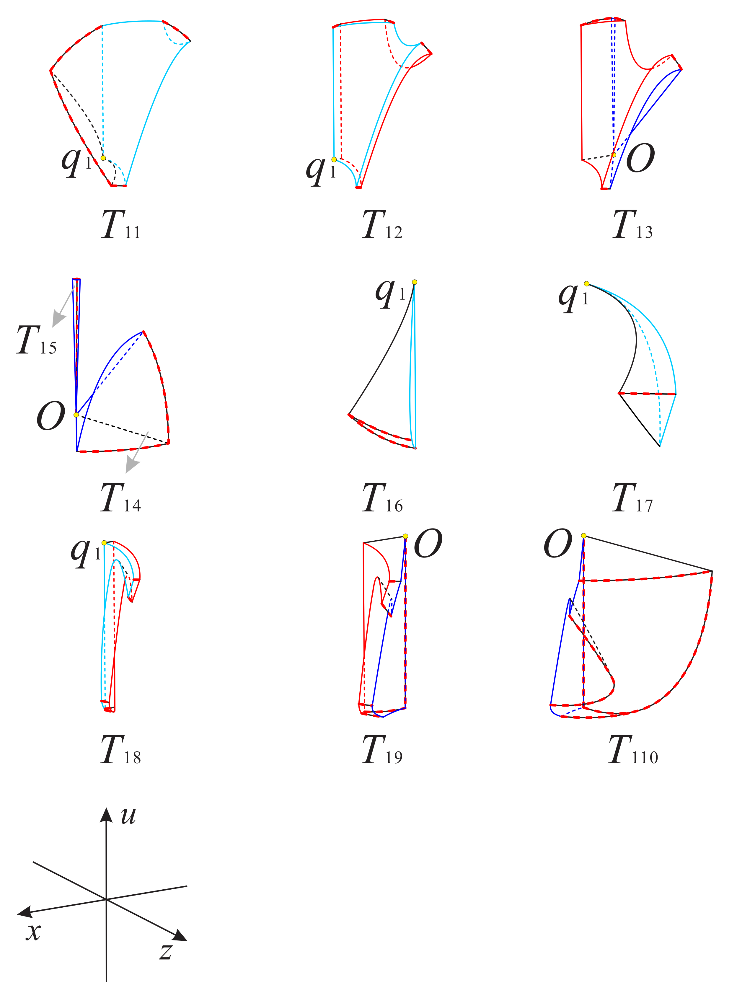
Table 1.
Equilibrium points for the different values of s, where , and .
| Values of s | Equilibrium Points |
|---|---|
| and are unstable nodes, is an unstable saddle | |
| is an unstable node, is an unstable saddle-node | |
| and are unstable nodes, is an unstable saddle | |
| is an unstable saddle-node, is an unstable node | |
| is an unstable saddle, and are unstable nodes |
Table 2.
Equilibrium points for the different values of s, where , , , and .
| Values of s | Equilibrium Points |
|---|---|
| and are unstable nodes, is an unstable saddle | |
| is an unstable node, is an unstable saddle-node | |
| and are unstable nodes, is an unstable saddle | |
| and are unstable nodes, is a semi-hyperbolic unstable saddle | |
| and are unstable nodes, is stable node, and are unstable saddles | |
| and are unstable nodes, is a semi-hyperbolic unstable saddle | |
| and are unstable nodes, is an unstable saddle | |
| is an unstable saddle-node, is an unstable node | |
| is an unstable saddle, and are unstable nodes |
Table 3.
Finite equilibrium points for the different values of s, where , , , and .
| Values of s | Equilibrium Points |
|---|---|
| and are unstable nodes, is a saddle | |
| is an unstable node, and are non-hyperbolic equilibrium points | |
| and are unstable nodes, is a saddle | |
| and are unstable nodes, , and are non-hyperbolic equilibrium points | |
| and are unstable nodes, , and are saddles | |
| and are unstable nodes, , and are non-hyperbolic equilibrium points | |
| and are unstable nodes, is a saddle | |
| and are non-hyperbolic equilibrium points, is an unstable node | |
| is a saddle, and are unstable nodes |
Table 4.
Signs of functions , and in the subregions of .
| Functions | Positive | Negative |
|---|---|---|
Table 5.
Signs of functions , and in the subregions of .
| Functions | Positive | Negative |
|---|---|---|
Table 6.
Dynamical behavior in the twenty subregions.
| Subregions | Corresponding Region | Increase or Decrease |
|---|---|---|
Table 7.
Signs of functions , and in the subregions of .
| Functions | Positive | Negative |
|---|---|---|
Table 8.
Signs of functions , and in the subregions of .
| Functions | Positive | Negative |
|---|---|---|
Table 9.
Dynamical behavior in the nineteen subregions.
| Subregions | Corresponding Region | Increase or Decrease |
|---|---|---|
Table 10.
Signs of functions , and in the subregion of .
| Functions | Positive | Negative |
|---|---|---|
Table 11.
Dynamical behavior in the ten subregions.
| Subregions | Corresponding Region | Increase or Decrease |
|---|---|---|
Table 12.
Signs of functions , and in the subregion of .
| Functions | Positive | Negative |
|---|---|---|
Table 13.
Dynamical behavior in the ten subregions.
| Subregions | Corresponding Region | Increase or Decrease |
|---|---|---|
Publisher’s Note: MDPI stays neutral with regard to jurisdictional claims in published maps and institutional affiliations. |
© 2021 by the authors. Licensee MDPI, Basel, Switzerland. This article is an open access article distributed under the terms and conditions of the Creative Commons Attribution (CC BY) license (https://creativecommons.org/licenses/by/4.0/).
Share and Cite
MDPI and ACS Style
Gao, F.; Llibre, J. Global Dynamics of the Hořava–Lifshitz Cosmological Model in a Non-Flat Universe with Non-Zero Cosmological Constant. Universe 2021, 7, 445. https://0-doi-org.brum.beds.ac.uk/10.3390/universe7110445
AMA Style
Gao F, Llibre J. Global Dynamics of the Hořava–Lifshitz Cosmological Model in a Non-Flat Universe with Non-Zero Cosmological Constant. Universe. 2021; 7(11):445. https://0-doi-org.brum.beds.ac.uk/10.3390/universe7110445
Chicago/Turabian StyleGao, Fabao, and Jaume Llibre. 2021. "Global Dynamics of the Hořava–Lifshitz Cosmological Model in a Non-Flat Universe with Non-Zero Cosmological Constant" Universe 7, no. 11: 445. https://0-doi-org.brum.beds.ac.uk/10.3390/universe7110445
Note that from the first issue of 2016, this journal uses article numbers instead of page numbers. See further details here.