Quasi-Periodic Oscillatory Motion of Particles Orbiting a Distorted, Deformed Compact Object

Abstract

This work explores the dynamic properties of test particles surrounding a distorted, deformed compact object. The astrophysical motivation was to choose such a background as to constitute a more reasonable model of a real situation that arises in the vicinity of compact objects with the possibility of having parameters such as the extra physical degrees of freedom. This can facilitate associating observational data with astrophysical systems. This work’s main goal is to study the dynamic regime of motion and quasi-periodic oscillation in this background, depending on different parameters of the system. In addition, we exercise the resonant phenomena of the radial and vertical oscillations at their observed quasi-periodic oscillations frequency ratio 3:2 and show that the oscillatory frequencies of charged particles can be adequately related to the frequencies of the twin high-frequency quasi-periodic oscillations observed in some sources of the microquasar observational data.

1. Introduction

Quasi-periodic oscillations (QPOs) of X-ray power spectral density have been observed at low (Hz) and high (kHz) frequencies and were discovered in the eighties [1,2]. Quasi-period oscillations have also been observed in supermassive black hole light curves and, recently, the source went through burst alert telescope (BAT) onboard Swift. Their importance is due to the fact that QPOs, peak features in the X-rays observed from stellar-mass BHs and neutron stars, are likely to arise from quite near the compact object itself and exhibit frequencies that scale inversely with the black hole mass, which allows us to probe and study the nature of accretion in highly curved space–time (for a review, see for example [3]).

One of the first QPO models is the relativistic precession model (RPM) that identifies the twin-peak QPO frequencies with the Keplerian and periastron frequencies. In the past years, the RPM has served to explain the twin-peak QPOs in several LMXBs. However, this model has some difficulties explaining the relatively large observed high frequencies of QPO amplitudes and inferred existence of preferred orbits. To modify this model, the high frequencies QPOs (two-picks) are considered as the resonances between oscillation modes of the accreted fluid—the well-known ratio 3:2 epicyclic resonance model—identify the resonant frequencies with frequencies of radial and vertical epicyclic axisymmetric modes of disc oscillations. The correlation is a cost of resonant corrections to these frequencies. The secret of this 3:2 ratio has still not been clearly revealed, and the oscillations occur only in certain states of luminosity, and hardness.

In this paper, we are motivated by the success of the above models, and we assume the QPOs are caused by the fundamental epicyclic frequencies associated with orbital motion of the matter in the accretion disc and their combinations.

We present our work on the background of a distorted, deformed compact object which is static and axisymmetric. This background is the simplest generalization of the so-called $\mathrm{q}$-metric up to quadrupole moments [4]. This metric has two parameters, aside from the central object’s mass; namely the distortion parameter and the deformation parameter, where in the absence of one or the other, one can recover either the $\mathrm{q}$-metric or distorted Schwarzschild metric [5]. From a dynamical point of view, these parameters can be seen as perturbation parameters of the Schwarzschild space–time. We explain this metric briefly in Section 2. In this respect, the first static and axially symmetric solution with arbitrary quadrupole moment are described by Weyl [6]. Later, Erez and Rosen introduced a static solution with arbitrary quadrupole in prolate spheroidal coordinates [7]. Then, Zipoy and Voorhees introduced an equivalent form [8,9] and, later on, by representing this metric in terms of a new parameter $\mathrm{q}$, which is known as $\mathrm{q}$-metric [10]. This area of study has been discussed extensively in the literature and generalized in many respects [11,12,13,14], among many others.

There are several motives to study the circular motion of particles in this background. In the relativistic astrophysical study, it is assumed that astrophysical compact objects are described by the Schwarzschild or Kerr space–times. However, besides these setups, others can imitate a black hole’s properties, such as the electromagnetic signature. Thus, it is also possible that some astrophysical observations cannot be fitted within the general theory of relativity by using the Schwarzschild or Kerr metric [15]. Moreover, the astrophysical systems are not always isolated as they are surrounded by different kinds of matter and radiation. In a more realistic scenario, the rotation should be taken into account; however, the possibility of observed resonant oscillations when they occur in the inner parts of accretion flow has been directly demonstrated, even if the source of radiation is steady and perfectly axisymmetric [16]. Therefore, this work could serve to constitute a reasonable model of a real situation that arises in the vicinity of this compact object, where it is not always isolated, with the possibility of analytic analysis through exercising parameters of the model where they can be treated as the degrees of freedom of the system and link the model to the observations.

In this paper, we also investigate dynamics of test particles in this background. This discussion can approximate a diluted astrophysical plasma’s complex dynamics, where they can be located around the system.

The paper’s organization is as follows: Section 2 presents the background object and a study of the motion of test particles in this background. Section 3 explains epicyclic frequencies and stable circular geodesics. The parametric resonances are presented in Section 4. Finally, the conclusions are summarized in Section 5.

Throughout this work, we use the signature $(-,+,+,+)$ and geometric unit system $G=1=c$, unless otherwise specified. Latin indices run from 1 to 3, while Greek ones take values from 0 to 3.

2. Space–Time of a Distorted, Deformed Compact Object

In this work, we consider generalized $\mathrm{q}$-metric, which has $\mathrm{q}$-metric as the seed metric and considers the existence of a static and axially symmetric external distribution of matter in its vicinity up to quadrupole. By its construction, this metric is only valid locally [5]. The metric has this form

$$\begin{array}{cc}\hfill \mathrm{d}{s}^2& =-{\left(\frac{x-1}{x+1}\right)}^{(1+\alpha )}{e}^{2\widehat{\psi }}d{t}^2+M^2(x^2-1)e^{-2\widehat{\psi }}\hfill \\ \hfill & {\left(\frac{x+1}{x-1}\right)}^{(1+\alpha )}\left[{\left(\frac{x^2-1}{x^2-y^2}\right)}^{\alpha (2+\alpha )}{e}^{2\widehat{\gamma }}\right.\hfill \\ \hfill & \left.\left(\frac{d{x}^2}{x^2-1}+\frac{d{y}^2}{1-y^2}\right)+(1-y^2)d{\varphi }^2\right],\hfill \end{array}$$

(1)

where $t\in (-\infty ,+\infty )$, $x\in (1,+\infty )$, $y\in [-1,1]$, and $\varphi \in [0,2\pi )$. M is a parameter that can be identified as the mass of the body generating the field, which is expressed in the dimension of length. The function $\widehat{\psi }$ plays the role of gravitational potential, and the function $\widehat{\gamma }$ is obtained by an integration of the explicit form of the function $\widehat{\psi }$. These are given by

$$\begin{array}{cc}\hfill \widehat{\psi }& =-\frac{\beta }{2}\left[-3x^2{y}^2+x^2+y^2-1\right],\hfill \\ \hfill \widehat{\gamma }& =-2x\beta (1-y^2)\hfill \end{array}$$

(2)

$$\begin{array}{cc}\hfill & +\frac{{\beta }^2}{4}(x^2-1)(1-y^2)(-9x^2{y}^2+x^2+y^2-1).\hfill \end{array}$$

(3)

This metric contains three parameters, namely the total mass, $\alpha$ deformation parameter, and $\beta$ distortion parameter, which are taken to be relatively small and connected to the central object and the presence of external mass distribution, respectively. In the case of $\beta =0$, it turns to the $\mathrm{q}$-metric, and in the case of $\alpha =\beta =0$, the Schwarzschild metric is recovered. This metric may associate the observable effects to these parameters as new physical degrees of freedom. The relation between the prolate spheroidal coordinates $(t,x,y,\varphi )$ and the Schwarzschild coordinates $(t,r,\theta ,\varphi )$ is given by

$$\begin{array}{c}\hfill x=\frac{r}{M}-1,y=cos\theta .\end{array}$$

(4)

In addition, the related kinematic quantities in this background, specific energy, angular momentum, and Keplerian orbital frequency, respectively, read as

$$\begin{array}{cc}\hfill & E=e^{-\widehat{\psi }}\sqrt{{\left(\frac{x-1}{x+1}\right)}^{1+\alpha }\frac{x-S}{x-2S}},\hfill \end{array}$$

(5)

$$\begin{array}{cc}\hfill & L=\pm e^{-\widehat{\psi }}(1+x)\sqrt{{\left(\frac{x+1}{x-1}\right)}^{\alpha }\frac{S}{x-2S}},\hfill \end{array}$$

(6)

$$\begin{array}{cc}\hfill & \Omega =e^{2\widehat{\psi }}{\left(\frac{x-1}{x+1}\right)}^{\alpha }\sqrt{\frac{x-1}{{(x+1)}^3}\frac{S}{x-S}},\hfill \end{array}$$

(7)

where

$$S:=1+\alpha +\beta x-\beta x^3.$$

(8)

Furthermore, by analyzing the effective potential, we can have general properties of the dynamics of a particle in this background. The effective potential in the equatorial plane is given by this relation [4]:

$$\begin{array}{cc}\hfill V_{\mathrm{eff}}=& {\left(\frac{x-1}{x+1}\right)}^{(\alpha +1)}{e}^{2\widehat{\psi }}\hfill \\ \hfill & \left[ϵ+\frac{L^2{e}^{2\widehat{\psi }}}{M^2{(x+1)}^2}{\left(\frac{x-1}{x+1}\right)}^{\alpha }\right].\hfill \end{array}$$

(9)

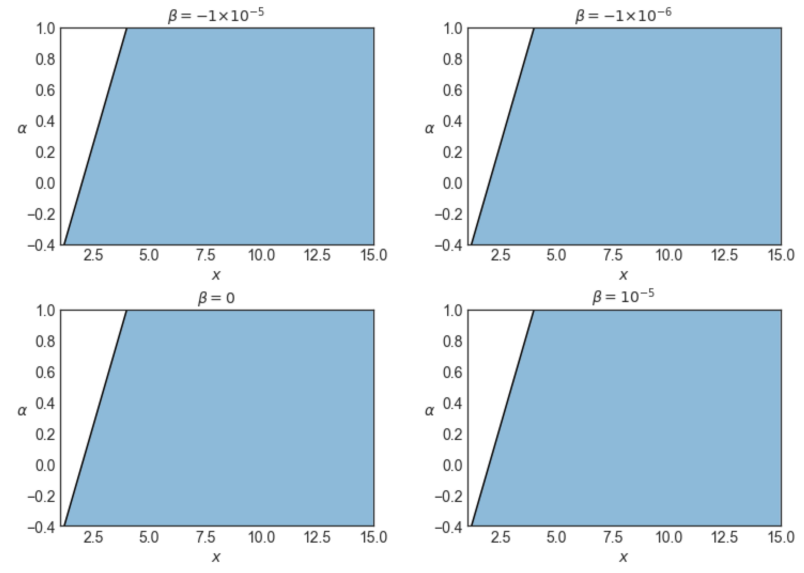
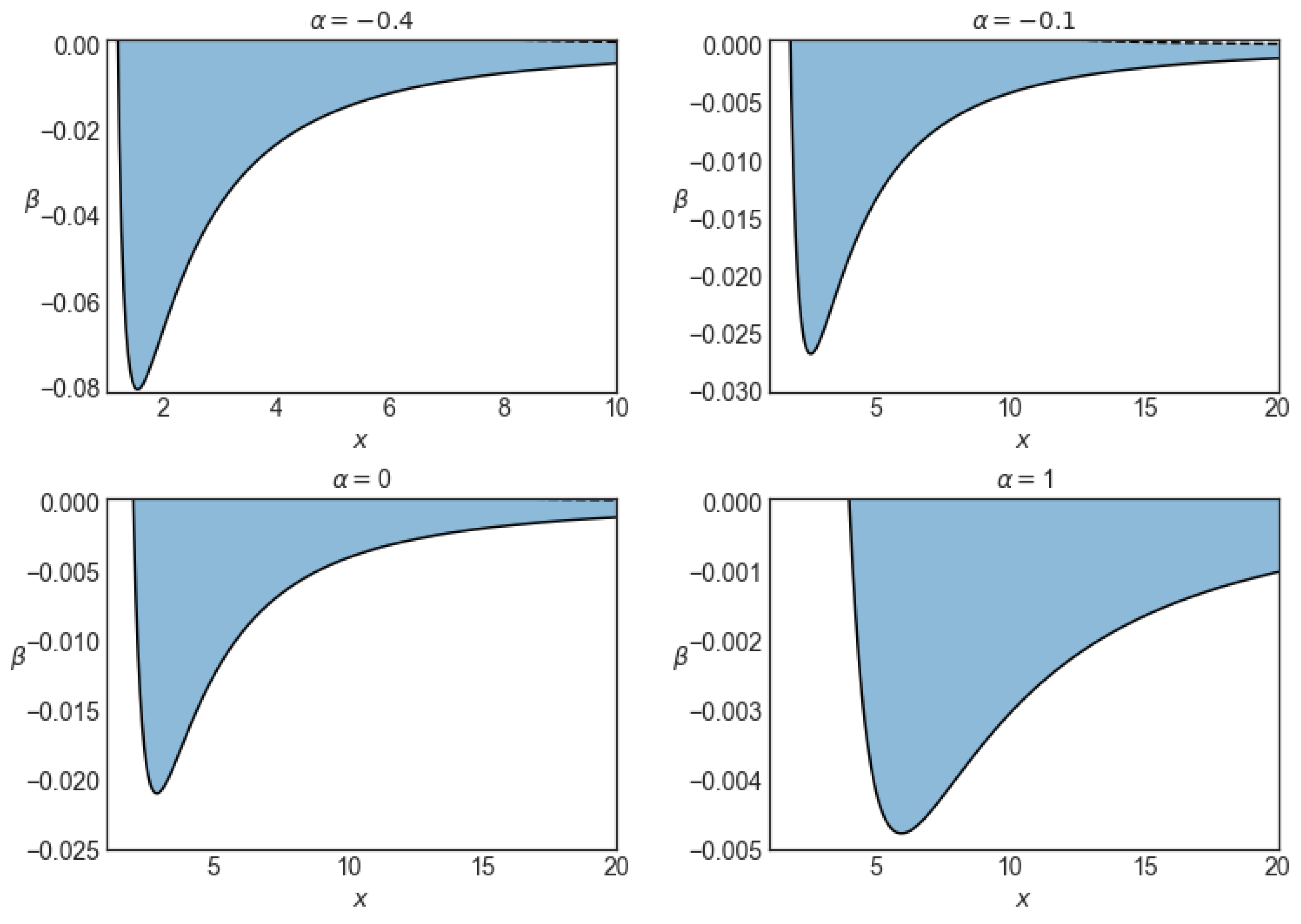
The domain of existence of the circular orbits in the equatorial plane is plotted in Figure 1 and Figure 2. In Figure 1, this domain is plotted in the ($x,\alpha$)-plane in terms of the distorted parameter $\beta$, while in Figure 2 this region is plotted in the ($x,\beta$)-plane for a range of values of the deformation parameter $\alpha$.

Following the standard procedure using effective potential, possible types of orbits, in general, dependent on the parameters $ϵ$, $\mathcal{E}$, L, $\alpha$, and $\beta$. However, in what follows, we only discussed bounded timelike trajectories as we are interested in studying oscillation of particle for a small perturbation of the orbit; however, the test particles’ motion can be chaotic in this background for some combinations of parameters $\alpha$ and $\beta$.

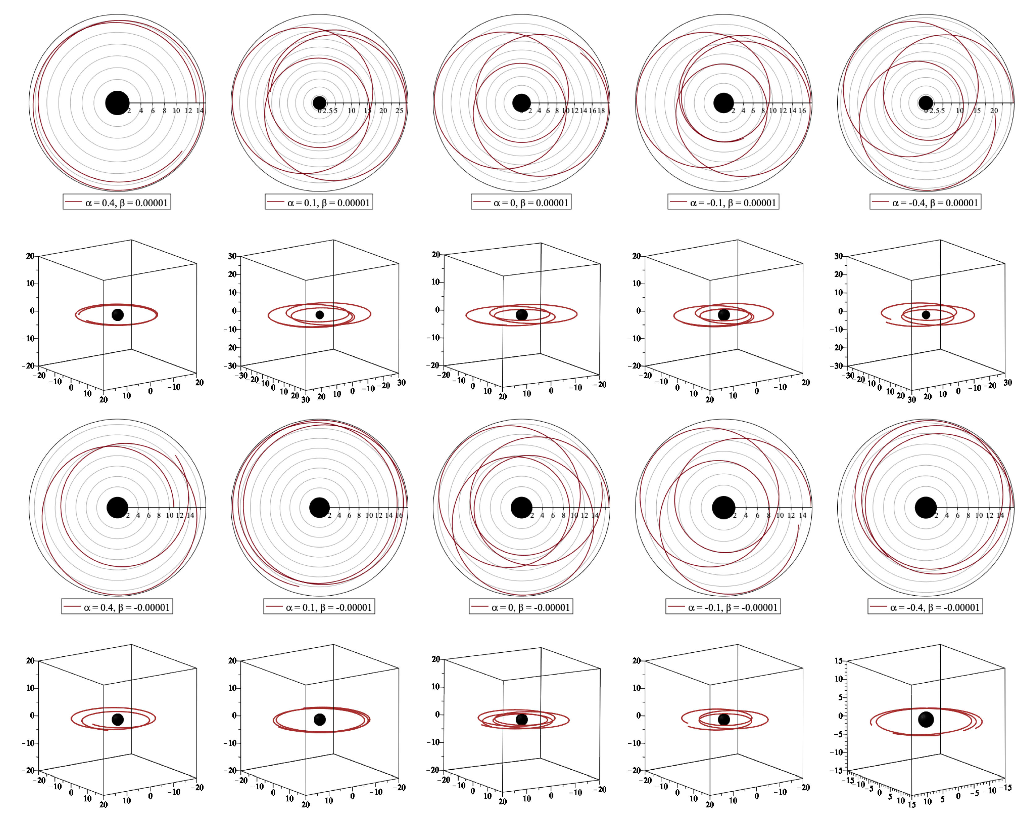
Figure 3 corresponds to the existence of both initial conditions on inner and outer boundaries, where particles trapped in some region form a toroidal shape around the central object. The trajectories for some choices of the parameters are plotted, where a rapid inspection shows that the trajectories of the particle noticeably change when the parameters change.

3. Epicyclic Frequencies and Stability of Circular Geodesics

In the accretion disc processes, a variety of oscillatory motions are generally expected. In this regard, circular and quasi-circular orbits seem to be crucial. In the study of the relativistic accretion disc, three frequencies are relevant. The Keplerian orbital frequency ${\nu }_K=\frac{\Omega }{2\pi }$, radial frequency ${\nu }_x=\frac{{\omega }_x}{2\pi }$, and the vertical frequency ${\nu }_y=\frac{{\omega }_y}{2\pi }$. A resonance between these frequencies can be a source of quasi-periodic oscillations that leads to chaotic and quasi-periodic variability in X-ray fluxes observations in many galactic objects.

In the relativistic precession model (RPM) of QPO, it is assumed that this oscillation caused by the epicyclic frequencies associated with the quasi-Keplerian motion in the accretion discs. In RPM, the upper frequency is defined as the Keplerian frequency ${\nu }_U={\nu }_K$ and the lower frequency is defined as the periastron frequency, i.e., ${\nu }_p:={\nu }_L=\pm ({\nu }_K-{\nu }_x)$. Their correlations are obtained by varying the radius of the associated circular orbit in a reasonable range. Within this framework, it is usually assumed that the variable components of the observed X-ray signal are placed in a bright localized spot or blob orbiting the compact object on a slightly eccentric orbit. Therefore, because of the relativistic effects, the observed radiation is supposed to be periodically modulated.

To study the stability of circular geodesics in the equatorial plane, we start by considering the geodesic equation for a test particle

$$\frac{d^2{x}^{\mu }}{d{s}^2}+{\mathsf{\Gamma }}_{\nu \rho }^{\mu }\frac{d{x}^{\nu }}{ds}\frac{d{x}^{\rho }}{ds}=0,$$

(10)

and substitute $(x=x_0,y=0)$ as we are in the equatorial plane. To describe the more general class of orbits that slightly deviate from the circular geodesics in the equatorial plane $x^{\mu }$, we consider this diffeomorphism $x^{\prime \mu }=x^{\mu }+{\xi }^{\mu }$. If we write the geodesic equation for this perturbation, by considering terms up to linear order in ${\xi }^{\mu }$, we obtain [17]

$$\frac{d^2{\xi }^{\mu }}{d{t}^2}+2{\gamma }_{\eta }^{\mu }\frac{d{\xi }^{\eta }}{dt}+{\xi }^{\eta }{\partial }_{\eta }{U}^{\mu }=0,$$

(11)

where

$$\begin{array}{cc}\hfill & {\gamma }_{\eta }^{\mu }={\left[2{\mathsf{\Gamma }}_{\eta \delta }^{\mu }{u}^{\delta }{\left(u^0\right)}^{-1}\right]}_{y=0},\hfill \end{array}$$

(12)

$$\begin{array}{cc}\hfill & U^{\mu }={\left[{\gamma }_{\eta }^{\mu }{u}^{\eta }{\left(u^0\right)}^{-1}\right]}_{y=0},\hfill \end{array}$$

(13)

where the 4-velocity for the circular orbits in the equatorial plane is $u^{\mu }=u^0(1,0,0,\Omega )$. Then, integration of the Equation (11) for the t and $\varphi$ components leads to

$$\begin{array}{cc}\hfill & \frac{d{\xi }^{\eta }}{dt}+{\gamma }_{\nu }^{\eta }{\xi }^{\nu }=0,\hfill \end{array}$$

(14)

$$\begin{array}{cc}\hfill & \frac{d^2{\xi }^x}{d{t}^2}+{\omega }_x^2{\xi }^x=0,\hfill \end{array}$$

(15)

$$\begin{array}{cc}\hfill & \frac{d^2{\xi }^y}{d{t}^2}+{\omega }_y^2{\xi }^y=0,\hfill \end{array}$$

(16)

where, in the first equation, $\eta$ can be taken t or $\varphi$, and

$$\begin{array}{cc}\hfill & {\omega }_x^2={\partial }_x{U}^x-{\gamma }_{\eta }^x{\gamma }_x^{\eta },\hfill \end{array}$$

(17)

$$\begin{array}{cc}\hfill & {\omega }_y^2={\partial }_y{U}^y.\hfill \end{array}$$

(18)

This system of equations describes the free radial phase and vertical oscillations of a particle around the circular geodesics1. The sign of frequencies ${\omega }_x^2$ and ${\omega }_y^2$ determine the dynamics and leads to having a circular orbit that is either stable or unstable. Indeed, even a tiny perturbation can cause a strong deviation from the unperturbed path.

In the Schwarzschild solution, these frequencies in spheroidal coordinates are given by

$$\begin{array}{cc}\hfill & {\omega }_x^2=\frac{1}{{(x+1)}^3}\left(1-\frac{6}{x+1}\right),\hfill \end{array}$$

(19)

$$\begin{array}{cc}\hfill & {\omega }_y^2=\frac{1}{{(x+1)}^3}.\hfill \end{array}$$

(20)

In Schwarzschild space–time, the stability of the circular orbits is determined only by the radial epicyclic frequency, since the vertical frequency coincides with the orbital frequency ${\omega }_y^2={\Omega }^2$. As is seen from the Equation (19), the vertical epicyclic frequency is a monotonically decreasing function of x, and we have ${\omega }_x^2<{\omega }_y^2={\Omega }^2$, and there also exists a periapsis shift for bounded quasi-elliptic trajectory, implying the effect of relativistic precession that changes the radius of the orbit [19]. Indeed, the ordering between frequencies contributes to the possible resonances that may occur in a given background. Furthermore, the behavior of the frequencies helps us to distinguish possible trajectories around a stable circular orbit.

These epicyclic frequencies in the background of a distorted and deformed compact object are written as

$$\begin{array}{cc}\hfill w_x^2=& A_x{\Omega }^2,\hfill \end{array}$$

(21)

$$\begin{array}{cc}\hfill w_y^2=& A_y{\Omega }^2,\hfill \end{array}$$

(22)

where

$$\begin{array}{cc}\hfill A_x=& \frac{e^{-2\tilde{\gamma }}{(1-1/x^2)}^{-\alpha (2+\alpha )}}{(x^2-1)}\hfill \\ \hfill & \left[2(2S-x)(S-x)-\frac{(x^2-1)}{S}(1+\alpha +2\beta x^3)\right],\hfill \end{array}$$

(23)

$$\begin{array}{cc}\hfill A_y=& \frac{e^{-2\tilde{\gamma }}{(1-1/x^2)}^{-\alpha (2+\alpha )}}{S}(1+\alpha +2\beta x^3),\hfill \end{array}$$

(24)

where S is given as before

$$S:=1+\alpha +\beta x-\beta x^3.$$

(25)

Note that these frequencies are measured regarding the proper time of a comoving observer. The signs of these fundamental frequencies provide a natural condition of having the valid domain of existence of circular and quasi-circular orbits. We explore these frequencies and the valid region more perspicaciously on Figure 4 and Figure 5.

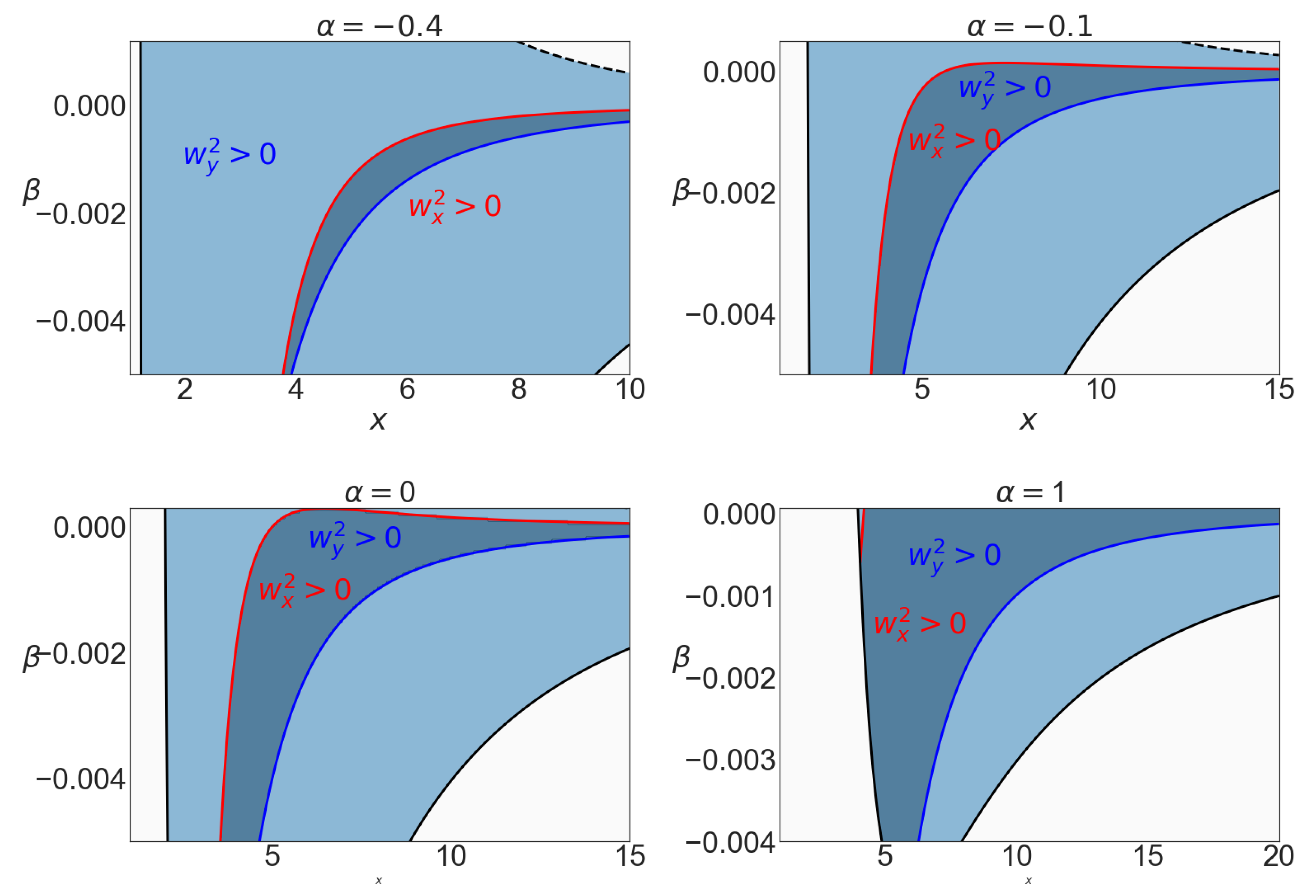
In Figure 4, the region of stability of the timelike circular geodesics is plotted in the $(x,\alpha )$-plane for different values of the distortion parameter $\beta$, and in Figure 5, in the $(x,\beta )$-plane for different values of the deformation parameter $\alpha$. In Figure 4, as the sign of radial frequency suggests: outside the red curve and in the blue region the timelike geodesics are unstable for radial perturbations but stable for the vertical ones. In Figure 5, both the curves $w_y^2=0$ and $w_x^2=0$ are depicted. The dark region is then bounded by these two curves and shows the stable domain. Comparing these two figures shows that the effect of parameter $\alpha$ is more profound than $\beta$. However, increasing $\beta$ tends to shrink the range of $\alpha$ in the valid region.

The interesting situation in this background, contrary to the Schwarzschild case, is the various ordering possibilities that arise among frequencies. For analyzing the order of magnitude of these frequencies, we analyze the frequency ratio

$$\frac{w_x^2}{w_y^2}=\frac{2S(2S-x)(S-x)}{(x^2-1)(1+\alpha +2\beta x^3)}-1.$$

(26)

These parameters $\beta$ and $\alpha$ are not independent of each other; fixing one of them restricts the other’s domain. For example, for a small enough parameter $\alpha$, we have this range of orders for parameter $\beta$

• $\alpha <0$: $-\mathcal{O}\left({10}^{-2}\right)<\beta <\mathcal{O}\left({10}^{-3}\right)-\mathcal{O}\left({10}^{-4}\right)$
• $\alpha >0$: $-\mathcal{O}\left({10}^{-3}\right)<\beta <\mathcal{O}\left({10}^{-4}\right)-\mathcal{O}\left({10}^{-5}\right)$.

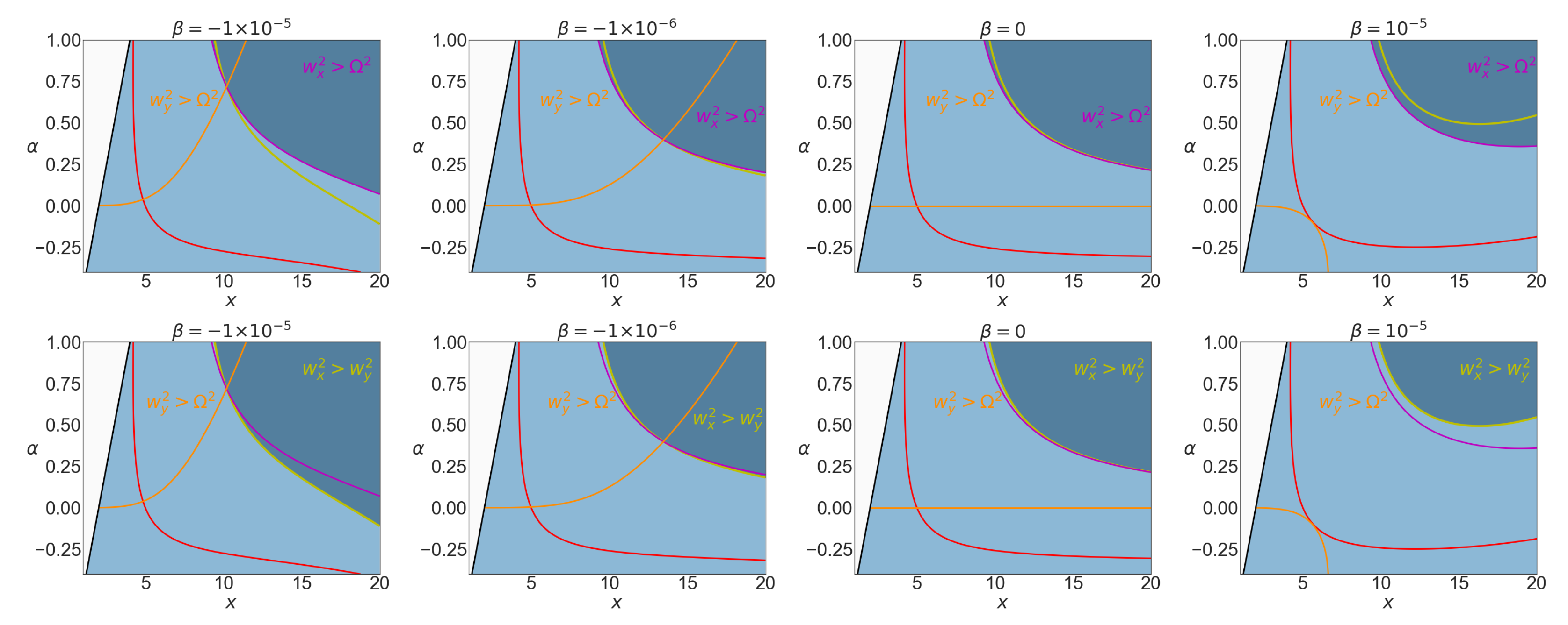
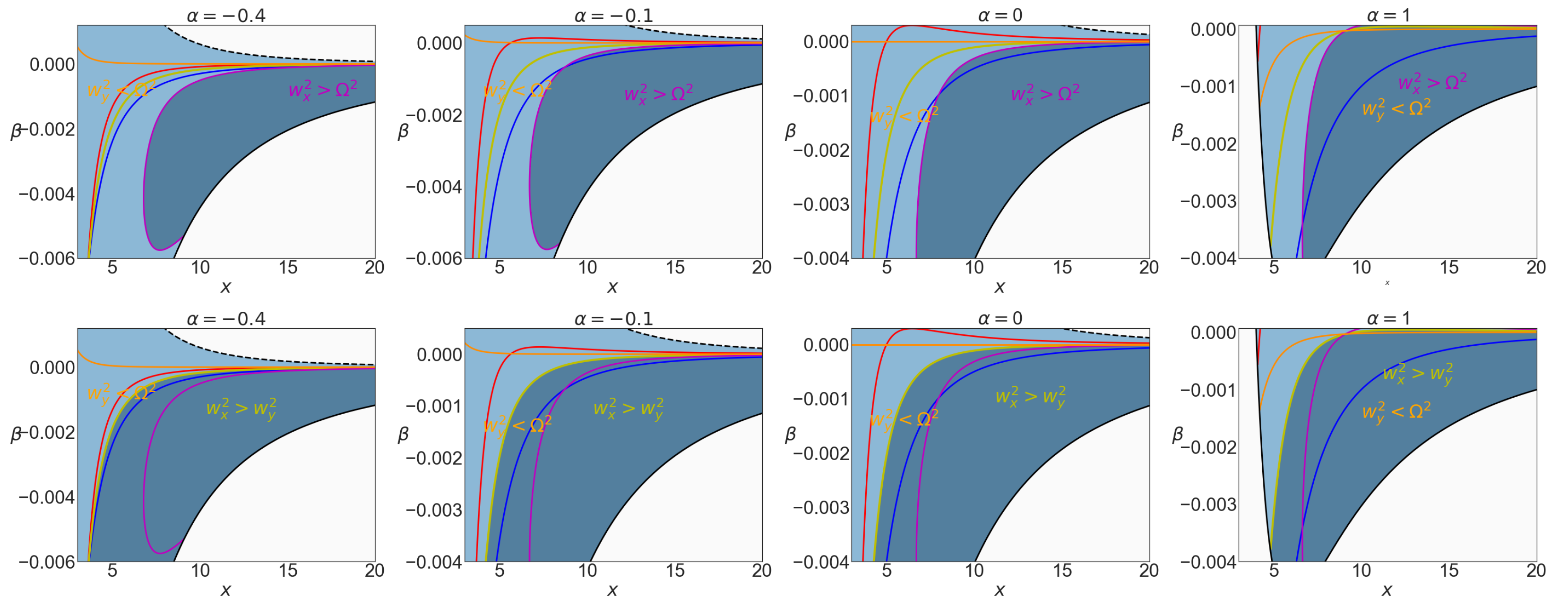
In Figure 6, the different epicyclic frequencies in the ($x,\alpha$)-plane for different values and signs of the distortion parameter $\beta$ are plotted. In addition, curves of $w_y^2={\Omega }^2$, $w_x^2={\Omega }^2$ and $w_x^2=w_y^2$ are specified. Moreover, in the first row, the dark area represents where $w_x^2>{\Omega }^2$, and in the second row, it represents where $w_x^2>w_y^2$. We illustrated both in one panel to ensure it would be easy to compare and analyze the behavior of different regions. In Figure 7, the different epicyclic frequencies are also presented in the ($x,\beta$)-plane for different values of the deformation parameter $\alpha$. In fact, this ordering is influenced by the signs and values of both parameters $\alpha$ and $\beta$.

By considering Figure 6 and Figure 7, we can extract interesting information about the order of the epicyclic frequencies in this background: in Figure 6, in the $(x,\alpha )$-plane, if we are interested in the order of the frequencies above the red line where $w_x^2$ and $w_y^2$ are both positives, we see that the ordering change after intersections. One appears when the red curve crossing the orange curve and the other one when the three yellow, pink, and orange curves cross each other, namely where we have ${\Omega }^2=w_y^2=w_x^2$.

Thus, the first possibility is above the red curve, where there is no intersection point, then we have $w_y^2>{\Omega }^2$. On the contrary, if a crossing point between the red and the orange appears, both situations $w_y^2>{\Omega }^2$ and $w_y^2<{\Omega }^2$ are possible. However, the existence of the second crossing point makes the order among the three frequencies even more varied. In the following, we present the order for different cases concerning different situations. In the second row of Figure 6, we can extract three different orderings:

(i)

from the red curve to the pink curve: $w_x^2<{\Omega }^2<w_y^2$;

(ii)

from the pink line to the yellow line: ${\Omega }^2<w_x^2<w_y^2$;

(iii)

from the yellow line to the top: ${\Omega }^2<w_y^2<w_x^2$.

In addition, for $\beta \le 0$ several different regions appear:

(i)

above the red curve and below the orange, three regions present:

(a)

below the pink and the yellow: $w_x^2<w_y^2<{\Omega }^2$;

(b)

above the yellow and below the pink (small area): $w_y^2<w_x^2<{\Omega }^2$;

(c)

above the yellow and the pink: $w_y^2<{\Omega }^2<w_x^2$.

(ii)

above the red curve and the orange one, three regions appear:

(a)

below the pink and the yellow: $w_x^2<{\Omega }^2<w_y^2$;

(b)

above the pink and below the yellow (small area): ${\Omega }^2<w_x^2<w_y^2$;

(c)

above the yellow and the pink: ${\Omega }^2<w_y^2<w_x^2$.

One can conclude the same results also by using Figure 7.

4. Parametric Resonances

Before the twin-peak HF QPOs were discovered in microquasars, this existence and ratio, also their rational ratio due to the resonances in quasi-Keplerian accretion discs, was expected [20,21]. Apparently, this fact is well supported by observations. In addition, this 3:2 ratio as the ratio of $({\nu }_U$:${\nu }_L)$ is seen most often in the twin HF QPOs in the LMXB containing microquasars.

In this section, we study this phenomena by means of parametric resonance and following the standard procedure utilizing the Mathieu’s equation [22]. This equation is a linear second-order ODE, which differs from the one corresponding to a harmonic oscillator in the existence of a periodic and sinusoidal forcing of the stiffness coefficient as $f\left(t\right)=f_0+f_{1}cos\left({\omega }_x^{2}t\right)$, and is given by

$$\frac{d^2{\xi }^y}{d{t}^2}+{\omega }_y^2\left[1+{\omega }_y^{2}hcos\left({\omega }_x^{2}t\right)\right]{\xi }^y=0$$

(27)

where $h=\frac{f_1}{f_0}\gg 0$ is the amplitude of the excitation (forcing) term, ${\nu }_x=\frac{{\omega }_x}{2\pi }$ is its excited frequency, and ${\nu }_y=\frac{{\omega }_y}{2\pi }$ is the natural, unexcited frequency.

It is well known that this setup performs free oscillation around the stable equilibrium case. If the stiffness term contains the parametric excitation, i.e., $f_1\ne 0$, the motion can stay bounded, which is referred to as stable, otherwise the motion becomes unbounded and is referred to as unstable.

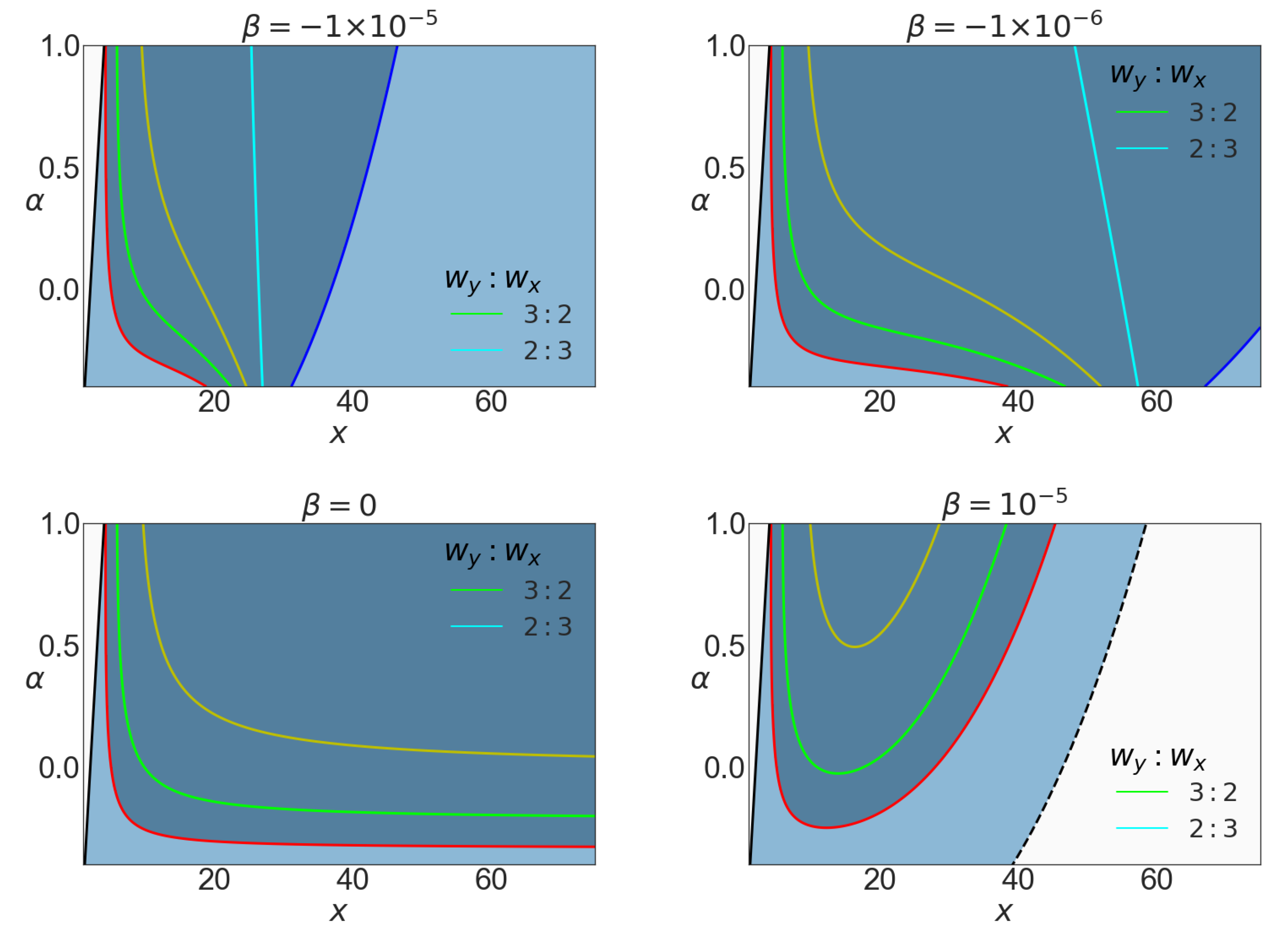
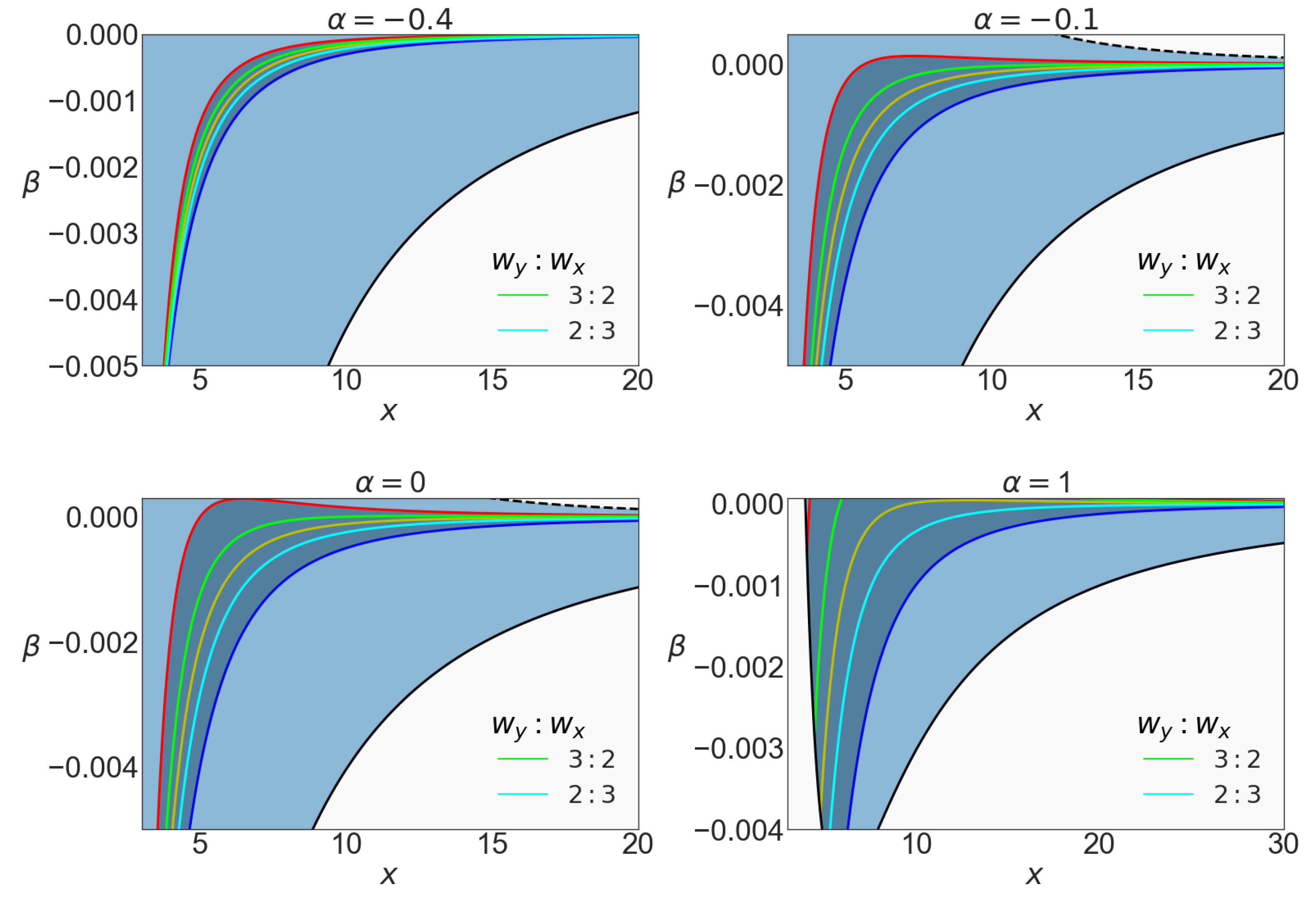
The resonance excitation arises for special values of frequencies. In contrast to the standard resonance epicyclic model, the oscillating test particles in this background allow both frequency ratios ${\nu }_y$:${\nu }_x=3$:2 and ${\nu }_y$:${\nu }_x=2$:3, which can be relevant in other observed data, such as in different twin frequencies observed in the microquasar GRS $1915+105$ (see, for example [23]). In Figure 8 and Figure 9, these resonance ratio for some chosen parameters are depicted. We can see that the 3:2 resonance in the physical range is always present, while it is not the case for this ratio 2:3. For instance, for a positive value of $\beta$, in the possible range for $\alpha$, the 2:3 resonance ration is not possible.

The QPO models are based on the frequencies of the quasi-circular geodesic motion. However, we should mention that considering nongeodesic effects, such as fluid pressure, can modify these models. In QPO models, one can identify the upper and lower frequencies $({\nu }_U,{\nu }_L)$ with different combinations of ${\nu }_x$ and ${\nu }_y$ such as $({\nu }_x,{\nu }_y)$, or $({\nu }_y,{\nu }_x)$, which can also produce the 3:2 ratio.

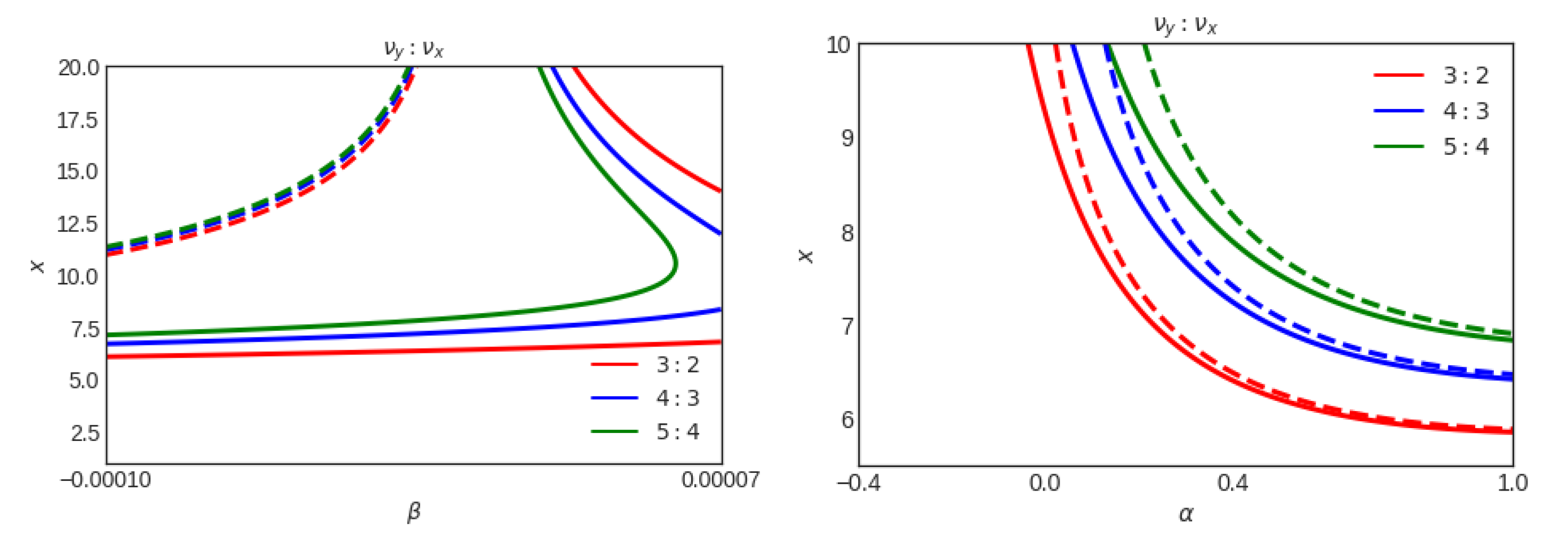
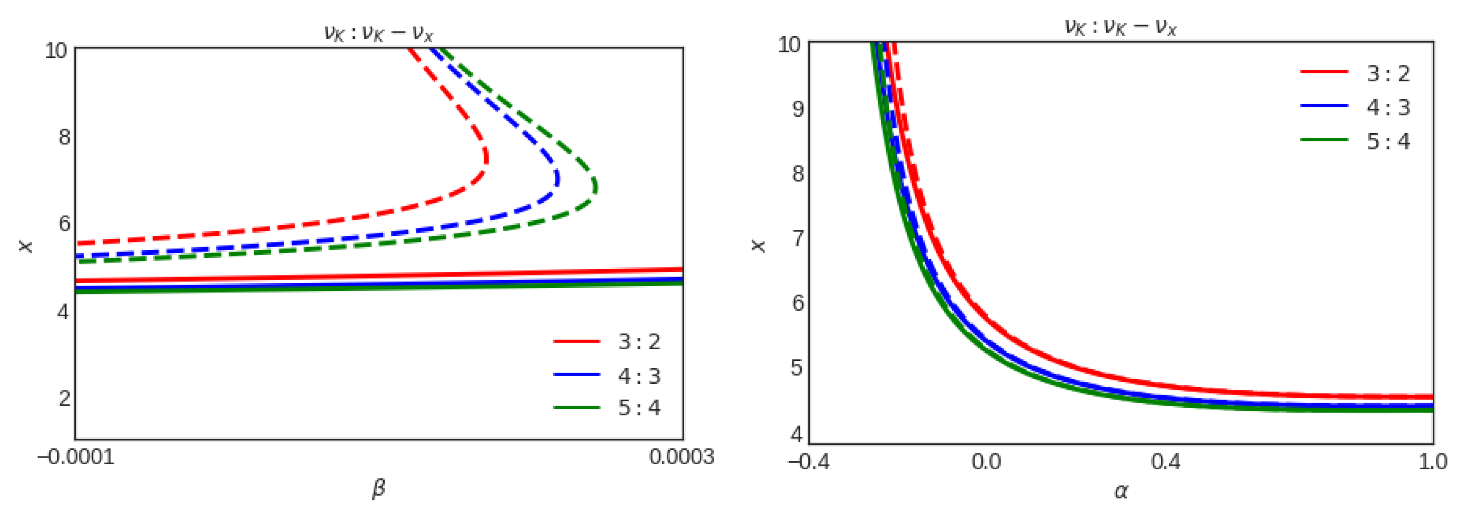
In Figure 10 and Figure 11, the location of the three ratios ${\nu }_U:{\nu }_L$ ={(3:2), (4:3), (5:4)} are plotted. In Figure 10, we consider one of the models so-called EP and study the resonance between the vertical epicyclic frequency, ${\nu }_U={\nu }_y$, and the radial one ${\nu }_L={\nu }_x$ with respect to $\beta$, and for two chosen values of $\alpha$, also with respect to $\alpha$, and are presented for two chosen values of $\beta$. In Figure 11, the plots present the RP model, which is one of the promising models and shows the resonance between the Keplerian epicyclic frequency ${\nu }_U={\nu }_K$ and the periastron frequency ${\nu }_L={\nu }_K-{\nu }_x$. In both figures, in the first row, we see that two radii satisfy the ratios ${\nu }_y:{\nu }_x$, and ${\nu }_K:{\nu }_K-{\nu }_x$. Moreover, increasing $\beta$ tends to push the radius of the resonances outward. In the second row, the behavior of the radius is not sensitive to the value of $\beta$ and is monotonically decreasing with the parameter $\alpha$.

In addition, in Figure 10 and Figure 11, the ratios of epicyclic frequencies at the maximum of ${\omega }_y$ are depicted. We see that the curves take their minimum at different radii depending on the choice of $\beta$. In all cases, the positive and negative values of $\beta$ almost take their maximum at the same ratios; however, further analysis reveals that this radius is smaller for its negative values. In addition, the maximum depend on the ratio; for example, we see that as this ratio becomes larger, the maximum shifted in the smaller radius.

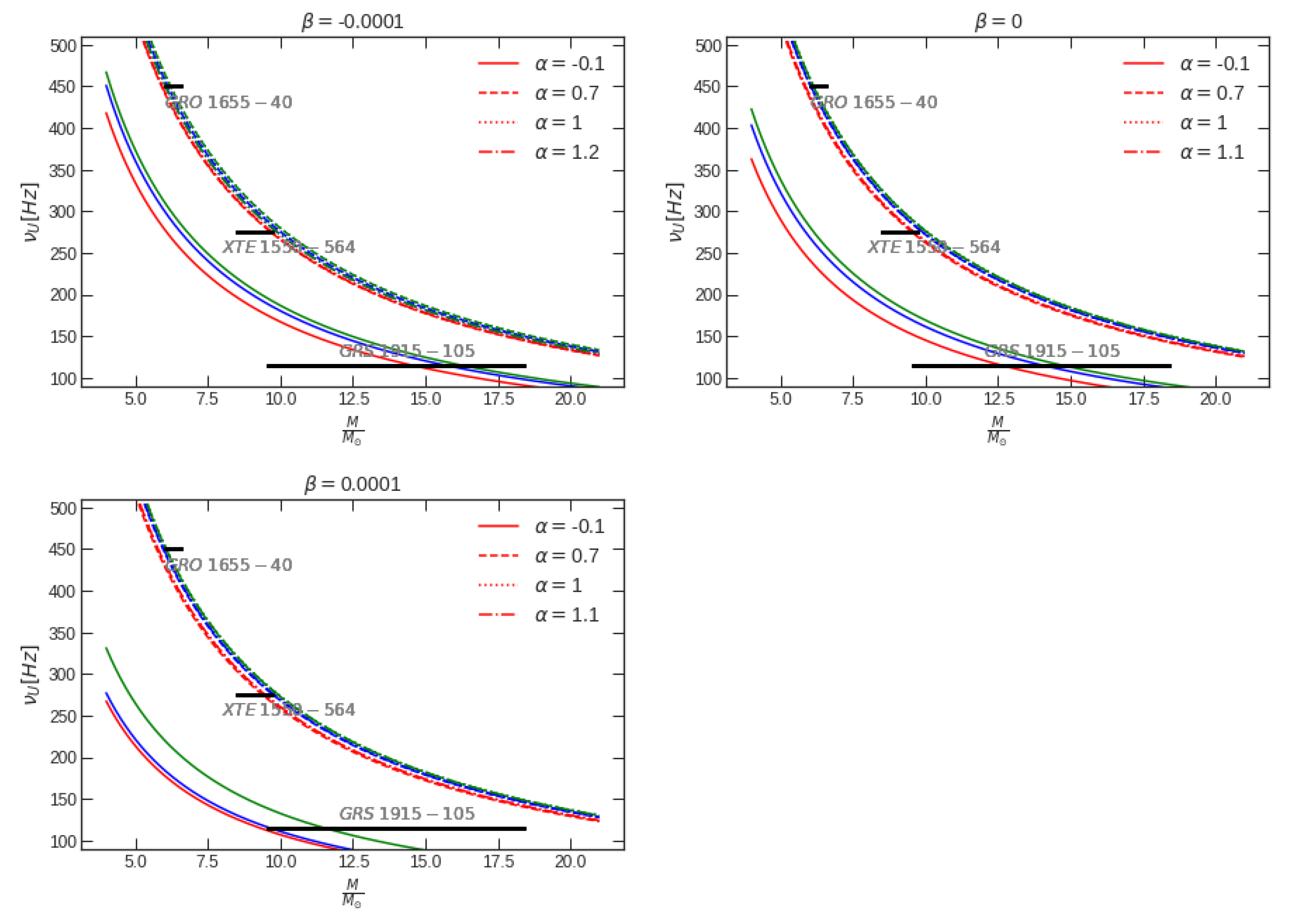
We also presented the result of fitting the oscillation frequencies to the observed frequencies data for the three microquasars GRS $1915+105$, XTE $1550-564$, and GRO $1655-40$ in Figure 12. While considering rotation may modify the radial profiles of the vertical and horizontal frequencies, these preliminary results show that the fitting can be conducted even for the fast rotating microquasar as GRS $1915+105$ and GRO $1655-40$. In fact, the work in progress shows that the positive $\alpha$ can play the role of the corotating Kerr, and its negative value the role of counter-rotating case in the part closer to the central object. However, we focus on the fitting in the case of a relatively slowly rotating XTE 1550 − 564 source, which is more compatible with our setup. As it shows, the parameter $\alpha$ is a more contributing factor. For vanishing $\alpha$, the result is in good agreement with previous studies [24,25]. Further analysis reveals that we have a better fit for $\alpha \in (0,1)$. In addition, we expect to have a better fit for positive values of $\beta$. As a result, in Figure 12, we see that there is a good agreement with the data for the ratio 3:2, which is the actual frequencies of the twin HF QPOs observed in this microquasars, and confirm the efficiency of the model. In general, the current results are encouraging and show improved accuracy in estimated parameters when attempting to fit the data.

5. Summary and Conclusions

This work investigated the dynamics of particles and quasi-periodic oscillation by studying the fundamental frequencies of circular motion around a deformed compact object up to the quadrupole. The metric is static, axisymmetric, and contains the distortion parameter $\beta$ related to the surrounding matter and deformation parameter $\alpha$ linked to the central object, which are briefly explained in Section 2. The dependency of these two parameters is reflected in the motion and epicyclic frequencies of particles that cause strong deviation from the corresponding quantities in the Schwarzschild case. In this respect, one can explore different orderings among fundamental frequencies and various possibilities to reproduce the ratio of 3:2, as well as other ratios via different combinations of parameters, which is not the case in either the Schwarzschild or in $\mathrm{q}$-metric.

In general, the resonant phenomena of the radial and vertical oscillations at their frequency ratio 3:2 for different parameters can be adequately related to the frequencies of the twin 3:2 HF QPOs observed in the microquasars GRS $1915+105$, XTE $1550-564$, and GRO $1655-40$, especially for $\alpha \in (0,1)$. The effect of parameters on the radial and vertical frequencies around a stable equatorial orbit is substantial. Moreover, different combinations can link to producing different effects of compact objects. In fact, this model may cover a variety of exciting applications in general relativity, gravitational waves and astrophysics.

A further step of this work can be considering rotation that leads to modifying the radial profiles of the vertical and radial frequencies, which is a work in progress. In addition, the magnetic field can serve as a fundamental input in this system to model more real astrophysical systems. One can also extend this work from a single particle to a complex system, such as accretion discs. Moreover, this model could serve as the initial conditions in future numerical simulations.

References

- Van der Klis, M. Millisecond Oscillations in X-ray Binaries. Annu. Rev. Astron. Astrophys. 2000, 38, 717–760. [Google Scholar] [CrossRef] [Green Version]
- McClintock, J.E.; Remillard, R.A. Black hole binaries. In Compact Stellar X-ray Sources; Cambridge University Press: Cambridge, UK, 2006; Volume 39, pp. 157–213. [Google Scholar]
- Stuchlík, Z.; Kološ, M.; Kovář, J.; Slaný, P.; Tursunov, A. Influence of Cosmic Repulsion and Magnetic Fields on Accretion Disks Rotating around Kerr Black Holes. Universe 2020, 6, 26. [Google Scholar] [CrossRef] [Green Version]
- Faraji, S. A generalization of q-metric. arXiv 2020, arXiv:2010.15723. Available online: https://ui.adsabs.harvard.edu/abs/2020arXiv201015723F (accessed on 31 August 2021).
- Geroch, R.; Hartle, J.B. Distorted black holes. J. Math. Phys. 1982, 23, 680–692. [Google Scholar] [CrossRef]
- Weyl, H. Zur Gravitationstheorie. Ann. Phys. 1917, 359, 117–145. [Google Scholar] [CrossRef]
- Erez, G.; Rosen, N. The Gravitational Field of a Particle Possessing a Multipole Moment; Technion—Israel Institute of Technology: Haifa, Israel, 1959. [Google Scholar]
- Zipoy, D.M. Topology of Some Spheroidal Metrics. J. Math. Phys. 1966, 7, 1137–1143. [Google Scholar] [CrossRef]
- Voorhees, B.H. Static Axially Symmetric Gravitational Fields. Physical Review. Phys. Rev. 1970, 2, 2119. [Google Scholar] [CrossRef]
- Quevedo, H. Mass Quadrupole as a Source of Naked Singularities. Int. J. Mod. Phys. 2011, 20, 1779–1787. [Google Scholar] [CrossRef] [Green Version]
- Geroch, R. Multipole Moments. II. Curved Space. J. Math. Phys. 1970, 11, 2580–2588. [Google Scholar] [CrossRef]
- Hansen, R.O. Multipole moments of stationary space-times. J. Math. Phys. 1974, 15, 46–52. [Google Scholar] [CrossRef]
- Quevedo, H. General static axisymmetric solution of Einstein’s vacuum field equations in prolate spheroidal coordinates. Phys. Rev. 1989, 39, 2904. [Google Scholar] [CrossRef]
- Manko, V.S. On the description of the external field of a static deformed mass. Class. Quantum Gravity 1990, 7, L209. [Google Scholar] [CrossRef]
- Abramowicz, M.A.; Kluźniak, W.; Lasota, J.P. No observational proof of the black-hole event-horizon. Astron. Astroph. 2002, 396, L31–L34. [Google Scholar] [CrossRef] [Green Version]
- Bursa, M.; Abramowicz, M.A.; Karas, V.; Kluźniak, W. The Upper Kilohertz Quasi-periodic Oscillation: A Gravitationally Lensed Vertical Oscillation. ApJ 2004, 617, L45–L48. [Google Scholar] [CrossRef]
- Aliev, A.N.; Galtsov, D.V.; Petukhov, V.I. Negative Absorption Near a Magnetized Black-Hole—Black-Hole Masers. Astrophys. Space Sci. 1986, 124, 137–157. [Google Scholar] [CrossRef]
- Wald, R.M. General Relativity; Oxford University Press: Oxford, UK, 1984. [Google Scholar]
- Stella, L.; Vietri, M. Quasi-Periodic Oscillations from Low-Mass X-ray Binaries and Strong Field Gravity. 2001. Available online: https://ui.adsabs.harvard.edu/abs/2001ASPC..234..213S (accessed on 31 August 2021).
- Strohmayer, T.E. Discovery of a 450 Hz QPO from the Microquasar GRO J1655-40 with RXTE. arXiv 2001, arXiv:astro-ph/0104487. [Google Scholar]
- Kluzniak, W.; Abramowicz, M.A. The physics of kHz QPOs—Strong gravity’s coupled anharmonic oscillators. arXiv 2001, arXiv:astro-ph/0105057. [Google Scholar]
- Macke, W. LD Landau and EM Lifshitz Mechanics. Vol. 1 of: Course of Theoretical Physics. 165 S. m. 55 Abb. Oxford/London/Paris 1960. Pergamon Press Ltd. Preis geb. 40 s. net. ZAMM—J. Appl. Math. Mech./Z. Angew. Math. Mech. 1961, 41, 392. [Google Scholar] [CrossRef]
- Lachowicz, P.; Czerny, B.; Abramowicz, M.A. Wavelet analysis of MCG-6-30-15 and NGC 4051: A possible discovery of QPOs in 2:1 and 3:2 resonance. arXiv 2006, arXiv:astro-ph/0607594. [Google Scholar]
- Kološ, M.; Stuchlík, Z.; Tursunov, A. Quasi-harmonic oscillatory motion of charged particles around a Schwarzschild black hole immersed in a uniform magnetic field. Class. Quantum Gravity 2015, 32, 165009. [Google Scholar] [CrossRef] [Green Version]
- Stuchlík, Z.; Kološ, M. Models of quasi-periodic oscillations related to mass and spin of the GRO J1655-40 black hole. Astron. Astroph. 2016, 586, A130. [Google Scholar] [CrossRef] [Green Version]
- Remillard, R.A.; McClintock, J.E. X-Ray Properties of Black-Hole Binaries. Annu. Rev. Astron. Astrophys. 2006, 44, 49–92. [Google Scholar] [CrossRef] [Green Version]
- Shafee, R.; McClintock, J.E.; Narayan, R.; Davis, S.W.; Li, L.X.; Remillard, R.A. Estimating the Spin of Stellar-Mass Black Holes by Spectral Fitting of the X-Ray Continuum. Astrophys. J. Lett. 2006, 636, L113–L116. [Google Scholar] [CrossRef]
Figure 1.
The domain of existence of circular orbits in the equatorial plane, ploted in the ()-plane. Lightlike orbits are located on the black curve, . Timelike orbits’ positions form the blue area, which is bound by the locus of the null geodesics and the dashed curve .
Figure 2.
Figure 3.
Timelike geodesic for different pairs of . The trajectories in the section and in the complete 3D are plotted. In the first column, both configurations have and . In the second column, both configurations have and . In the central column, both configurations have and . In the fourth column, both configurations have and . In the last one, both configurations have and .
Figure 4.
Stability of timelike circular orbits in the ()-plane. Timelike circular orbits exist in the light blue area. This region is bounded by the thick dark line . The red curve represents . The area depicted by the blue-gray region shows the domain of stability. In the chosen range, in the entire light blue region. Timelike orbits are stable above the red curve with respect to vertical perturbations and radial perturbations. On the contrary, below the red curve and in the light blue region, the timelike geodesics are stable with respect to vertical perturbations but unstable with respect to radial perturbations.
Figure 5.
Stability of the timelike circular orbits in the ()-plane. Timelike circular orbit exists in the light blue area. This region is bounded by the thick dark line and the dashed line . The blue curve represents and the red one . The blue-gray region shows the stability domain with respect to chosen parameters.
Figure 6.
The different epicyclic frequencies in the ()-plane are examined. On all the plots, the yellow line depicts , the pink line shows , and the orange line is . The light blue area corresponds, as in Figure 4 and Figure 5, to the area where circular orbits exist (bounded by the thick black line ), and above the red line, the orbit is stable with respect to perturbations in both directions. In the panel, in the first row, the darker blue area satisfies . In the second row, the darker blue area satisfies . By considering the first and second rows together, one can have different ordering for these frequencies.
Figure 7.
The different epicyclic frequencies in the ()-plane are examined. As in Figure 4 and Figure 5, the red line shows and the blue line . On all plots, the yellow line depicts , the pink line shows , and the orange line is . The light blue area corresponds, as in Figure 4 and Figure 5, to the area where circular orbits exist (bounded by the thick black line and the dashed line ). Between the blue and the red line, when the red line is above the blue one, orbits are stable with respect to the perturbations in both directions. In this panel, in the first row, the darker blue area satisfies . In the second row, the darker blue area satisfies . By considering the first and second rows together, one can have different ordering for these frequencies.
Figure 8.
The light blue area depicts the region of existence of the circular orbits. This region is bounded by the thick black curve and the dashed line . The blue-gray region shows the stability of the orbit with respect to vertical and radial perturbations. This area is bounded by the blue curve () and the red curve (). In this -plane, the lime curve shows where we have and the light cyan curve .
Figure 9.
The light blue area depicts the region of existence of the circular orbits. This region is bounded by the thick black curve and the dashed line . The blue-gray region shows the stability of the orbit with respect to vertical and radial perturbations. This region is bounded by the blue () and the red () curves. The lime curve shows the resonance and the light cyan curve, shows the resonance .
Figure 10.
The first panel shows the location of three cases of resonances between vertical and radial epicyclic frequencies with respect to . The thick line shows and the dashed line . The second panel represents the location of three cases of resonances between the vertical and the radial epicyclic frequencies with respect to . The thick line shows and the dashed line .
Figure 11.
The first panel shows the location of three epicyclic resonances between the Keplerian epicyclic frequency and the periastron frequency as a function of . The thick line represents and the dashed line . The second one shows the location of three epicyclic resonances between the Keplerian epicyclic frequency and the periastron frequency as a function of . The thick line represents and the dashed line .
Figure 12.
Representation of the upper oscillation frequency at the resonance radius for different ratios related to Figure 11. We compared the frequency to the mass limits of microquasars obtained by observations. Their characteristics are given in Table 1. They are plotted for , and , and different values of . The colors represent the same ratio as Figure 11.
Publisher’s Note: MDPI stays neutral with regard to jurisdictional claims in published maps and institutional affiliations. |
© 2021 by the authors. Licensee MDPI, Basel, Switzerland. This article is an open access article distributed under the terms and conditions of the Creative Commons Attribution (CC BY) license (https://creativecommons.org/licenses/by/4.0/).
Share and Cite
MDPI and ACS Style
Faraji, S.; Trova, A. Quasi-Periodic Oscillatory Motion of Particles Orbiting a Distorted, Deformed Compact Object. Universe 2021, 7, 447. https://0-doi-org.brum.beds.ac.uk/10.3390/universe7110447
AMA Style
Faraji S, Trova A. Quasi-Periodic Oscillatory Motion of Particles Orbiting a Distorted, Deformed Compact Object. Universe. 2021; 7(11):447. https://0-doi-org.brum.beds.ac.uk/10.3390/universe7110447
Chicago/Turabian StyleFaraji, Shokoufe, and Audrey Trova. 2021. "Quasi-Periodic Oscillatory Motion of Particles Orbiting a Distorted, Deformed Compact Object" Universe 7, no. 11: 447. https://0-doi-org.brum.beds.ac.uk/10.3390/universe7110447
Note that from the first issue of 2016, this journal uses article numbers instead of page numbers. See further details here.