Particle-in-Cell Simulations of Astrophysical Relativistic Jets

Abstract

Astrophysical relativistic jets in active galactic nuclei, gamma-ray bursts, and pulsars is the main key subject of study in the field of high-energy astrophysics, especially regarding the jet interaction with the interstellar or intergalactic environment. In this work, we review studies of particle-in-cell simulations of relativistic electron–proton ($e^{-}-p^{+}$) and electron–positron ($e^{\pm }$) jets, and we compare simulations that we have conducted with the relativistic 3D TRISTAN-MPI code for unmagnetized and magnetized jets. We focus on how the magnetic fields affect the evolution of relativistic jets of different compositions, how the jets interact with the ambient media, how the kinetic instabilities such as the Weibel instability, the kinetic Kelvin–Helmholtz instability and the mushroom instability develop, and we discuss possible particle acceleration mechanisms at reconnection sites.

Contents
1. Introduction.........................................................................................................................................................................	2
1.1. Astrophysical Jets......................................................................................................................................................	2
1.2. The TRISTAN Code...................................................................................................................................................	2
1.3. Particle-in-Cell Approach and Plasma Instabilities...............................................................................................	3
2. Microscopic and Macroscopic Processes in Plasma Jets................................................................................................	5
3. PIC Simulations...................................................................................................................................................................	6
3.1. Unmagnetized Jets.....................................................................................................................................................	6
3.1.1. Self-Consistent Synthetic Spectra from Shocks...........................................................................................	6
3.1.2. Shear Velocity Simulations with the Slab Model and Cylindrical Jets.....................................................	8
3.1.3. Global Simulations of Unmagnetized Relativistic Jets..............................................................................	9
3.2. Magnetized Jets.........................................................................................................................................................	12
3.2.1. Topology of Relativistic Helical Jets............................................................................................................	12
3.2.2. Global Simulations with Helical Jets and Large Radii..............................................................................	14
3.2.3. Global Jet Simulations with a Toroidal Magnetic Field and a New Injection Scheme...........................	18
4. Summary..............................................................................................................................................................................	22
References................................................................................................................................................................................	23

1. Introduction

1.1. Astrophysical Jets

Plasma is one of the four fundamental states of matter while omnipresent throughout the Cosmos. Astrophysical plasmas in the form of relativistic jets are observed in many astrophysical energetic sources, e.g., pulsars, Gamma-ray Bursts (GRB), and Active Galactic Nuclei (AGN) [1,2,3]. Our understanding of the formation of jets, their interaction with the interstellar and intergalactic medium, and the consequent observable properties such as polarization and spectra from these astrophysical sources still remain limited [4].

The associated accretion disks and X-ray emissions observed from a plethora of high-energy sources suggest that there might be combinations of different mechanisms associated with many high-energy astrophysical sources. The transfer of the enormous amount of energy transferred from a generating black hole to a jetted plasma can be explained via two early theories: (i) the Blandford–Znajek process [5] describes how the energy from magnetic fields in relativistic jets is extracted from around an AGN accretion disk by the magnetic fields’ dragging and twisting as the black hole spins, which as a consequence launches relativistic material by the tightening of the magnetic field lines; (ii) Punsly and Coroniti [6] argued that the steady-state solutions of Blandford and Znajek, where the inertia of plasma particles was completely ignored while their electric charges remained accounted for as if in a perfectly conducting medium, were lacking causal connectivity and therefore could not hold in a time-dependent framework. Therefore, as a counter theory, the work of [6] proposed an alternative where the inertia of plasma particles was paramount, which resembled the theory of the so-called “Penrose-mechanism” [7] and where the energy is extracted from a rotating black hole by frame dragging.

Most of the jets are collimated, and most of them extend between several thousands up to millions of parsecs [1]. Observations show that jets are symbiotic with the activity of central black holes in AGN [8] and in other sources such as in GRBs [9], as well as in pulsars [3]. Among these highly energetic jetted sources, two of them, the GRBs and blazars—the latter being a class of AGNs with a relativistic jet directed nearly towards an observer—produce the brightest electromagnetic phenomena [10]. Relativistic jets exhibit a wide range of plasma phenomena, such as the generation or decay of magnetic fields, turbulence, magnetic reconnection, and propagation in the interstellar or intergalactic medium. In the dynamic environment of jetted sources, it is theorized that particle acceleration occurs via different mechanisms, which may be able to achieve the highest level of energies resulting in the observed cosmic-ray spectrum.

1.2. The TRISTAN Code

Since the 1950s, Particle-In-Cell (PIC) simulations have been used by research scientists. Buneman was one of the first prominent scientists in the field of plasma electrodynamics who contributed greatly to the PIC development methods. In 1993 [11], the PIC code named TRIdimensional STANford (TRISTAN) was introduced, which was a relativistic code designed to simulate the solar wind interactions with the Earth’s magnetosphere. TRISTAN is the base for several other PIC code versions [12,13,14], as it has been advanced using a Message Passage Interface (MPI). Further development over the years resulted in a highly sophisticated version of the code used by several research groups, designed to investigate relativistic jets with toroidal and poloidal magnetic fields [15,16,17,18,19,20,21].

The original version of TRISTAN has been parallelized with MPI by us, see, e.g., [13,22], optimized for speed and improved to efficiently handle small-scale numerical noise. This version, therefore, called TRISTAN-MPI, is designed to be flexible and to perform well on different computational platforms including user control over a number of optimization features. One example is the splitting of large loops into segments, for which the relevant variable can be simultaneously held in the processor cache, thus avoiding memory access over the system bus. Another example is the periodic resorting of particles, improving the speed of memory IO.

TRISTAN-MPI has been running in several large high-performance computing facilities such as Kraken, Ranger, etc., which are located at the Computer Centers of the National Science Foundation (NSF) [22]. The code has been performed on the Pleiades and Columbia systems of NASA Advanced Supercomputing (NAS). Note that the validation tests showed that this code has an excellent scalability, provided the memory load per core is kept above ≈100 MB. The TRISTAN-MPI is well optimized up to ten thousand (10,000) cores, and very large simulations for astrophysical jets have been performed using 556 nodes with 10,000 cores on Pleiades at NASA, reported in [17].

Currently, there are more than a dozen different PIC codes developed by researchers (e.g., EPOCH, PICCANTE, VPIC, etc.), several of which are publicly available, which has allowed a much broader part of the astrophysical community to conduct research in this exciting computational field. TRISTAN-MPI is not publicly available, but can be provided upon request along with simulation data. For further details, see our review work [23]. In this paper, we present a series of past and recent relativistic PIC simulation studies, performed for different electron–proton and electron–positron unmagnetized and magnetized jets, using the 3D TRISTAN-MPI code, with different simulation system dimensions, and we validate our results comparatively, addressing also the prospects for further studies.

1.3. Particle-in-Cell Approach and Plasma Instabilities

As previously mentioned, already during the 1950s, the first PIC method simulating plasma environments began with the brilliant effort of a few scientists such as Buneman, Hockney, Birdsall, and Dawson [11]. In the PIC method, the plasma charged particles interact only with the electromagnetic fields that are produced by the particles themselves (in their motion). The PIC method is employed to solve plasma kinetic (microscopic) processes. See more details in [23].

Recently, with the advancement of supercomputer facilities and PIC algorithms, PIC simulation methods have become a compliment to the fluid method, with the addition of kinetic processes. Whilst fluid method—hydrodynamic (HD) and/or magnetohydrodynamic (MHD) approach—models calculate densities, concentrations, or generally averaged quantities, the advantage of the PIC approach, often combined with Monte Carlo methods, is that it traces individual particles and is therefore able to capture rare events that would not be seen in fluid simulations [24]. We hence make a distinction here so as to understand the difference between the fluid approach and the PIC approach: Fluid models (e.g., with MHD simulations) cannot address the kinetic properties of a plasma. On the other hand, the PIC method approaches in full detail the kinetic plasma aspect with the intent of addressing the developed instabilities and particle acceleration mechanisms, which we discuss in more detail in this paper.

In the field of the PIC approach, it is especially challenging to integrate microscopic physics into global, large-scale dynamics, which is crucial to understanding, e.g., the full dynamics of astrophysical jets. Large PIC simulations are prone to and dependent on our society’s technological progress. The power of supercomputers is the key to their performance. PIC simulations require a very large memory; nevertheless, since supercomputers’ power is based on very small transistors, the rate of which is growing exponentially, doubling every two years (the so-called Moore’s law), many researchers already have moved into the full 3D simulations [25]. We should however bear in mind that the miniaturization trend of transistors will at some point come to an end due to overwhelming quantum effects. This prospect calls for the need for new technological solutions.

Rayburn (1977) [26] was the first to conduct a numerical study of astrophysical jets with a PIC code. In this work, the fluid of the jet was assumed to be given by a number of macroparticles. The computational grid consisted of just 10 × 20 grid cells and 16 particles/cell. That study concerned an injection aperture and the structure created through the interaction of a 2D uniform supersonic cylindrical nonrelativistic and unmagnetized flow with an external medium of uniform density. In that work, they observed a rarefied cocoon around the simulated jet, and they confirmed the generation of two shocks according to the prior works of [27], where a forward bow shock was driven by the jet into the external gas and a reverse shock, which terminated the supersonic flow of the jet itself.

Norman et al. (1981) [28] used a nonrelativistic 2D (HD) model to investigate the formation of jets from gravitationally bound clouds. That model used a finite difference code on a 40 × 40 grid. It is interesting to note that this, in its infancy, did not agree with the expected theoretical model; nevertheless, the findings opened the way toward newly discovered physics, and they have shed light onto a much better understanding of the nature of astrophysical plasmas.

Since astronomical observations confirmed that the AGN jets are magnetized relativistic plasmas, this prompted the need for codes that could handle such complex environments. The work of [29] was one of the first to carry out simulations of magnetized nonrelativistic jets with a numerical scheme for the axisymmetric MHD code, and many others followed since then, developing fully Relativistic MHD (RMHD) codes investigating their propagation and properties [30]. Currently, General Relativistic MHD (GRMHD) codes are used to study more realistic astrophysical jets.

Many instabilities occur when very-high-energy (relativistic) plasma jets interact with their environment. These instabilities are responsible for the acceleration of particles. Specifically, it is shown that in unmagnetized jets, the so-called Weibel Instability (WI) [31] is generated in relativistic shocks resulting in acceleration of particles. Other instabilities such as the kinetic Kelvin–Helmholtz (kKHI) and the Mushroom Instability (MI) are driven by the shear velocity at the boundary between the jet and the ambient medium. These instabilities also contribute to the acceleration of particles [32]. As a rule of thumb, kKHI is generated along the jet’s velocity. MI is excited in the direction perpendicular to it. It is standard that for an electron–positron jet, both kKHI and MI generate an AC magnetic field, whilst an electron–proton jet generates a DC magnetic field.

Except for the standardized Fermi acceleration mechanism, which is a stochastic process, another possible mechanism of particle acceleration is the so-called magnetic reconnection. This is a process where the magnetic topology of a given astrophysical site is rearranged and the magnetic energy present is converted into thermal and kinetic particle energy. Magnetic reconnection is directly observed in solar and planetary magnetospheric plasmas, and it is often assumed to be an important mechanism of particle acceleration especially in astrophysical extragalactic environments such as AGN and GRB jets [33,34,35,36,37,38,39,40,41,42,43,44,45,46]. Particle acceleration was found to occur due to Fermi mechanisms, but also due to magnetic reconnection, where the so-called Harris model in slab geometry was adapted [21,47,48,49,50,51,52,53,54]. Nevertheless, these studies were not realistically directly applicable to astrophysical relativistic jets, since observations [3,55], as well as MHD modeling [56] suggest that the magnetic field topology is predominantly helical (with poloidal and toroidal fields).

PIC simulations have been applied to tackle the study of instabilities in unmagnetized and magnetized relativistic jets [33,36,39,40,41,43,44,45,57,58,59,60]. PIC simulations of [15,20], which we discuss in Section 3, investigate the development of instabilities and the conditions of magnetic reconnection in relativistic jets with helical and toroidal magnetic fields. Other PIC simulations of [61] of a single flux rope showed that the jet undergoes internal kink instabilities, indicating the signatures of magnetic reconnection. Moreover, the RMHD simulations of [62,63] showed that helical fields develop kink instabilities. Recently, References [64,65] showed that in relativistic strongly magnetized jets with helical magnetic fields, the formation of highly tangled magnetic fields was due to the development of the kink instability along with a large-scale inductive electric field, promoting the rapid energization of particles.

The evolution of cylindrical jets (with helical or toroidal magnetic fields) is an important framework for studying instabilities and particle acceleration [19,66,67] within the jet. In the PIC simulation studies that we present in Section 3, the system length used was large enough to accommodate several instability modes (kKHI or WI) in the linear, but also in the nonlinear stage. For example, in the very recent PIC simulations of [15] for electron–proton and electron–positron jets, we clearly discerned different growing instabilities developing in the linear and nonlinear stage.

Global 3D PIC simulation studies for unmagnetized jets were for the first time performed by us in [17,68,69], which allowed a detailed investigation of the complex kinetic processes and associated phenomena in relativistic jets. Furthermore, PIC simulations for relativistic jets containing helical magnetic fields were also for the first time conducted by [67], followed by a series of spatiotemporally advanced simulation studies in, e.g., [15,18,19,20,70], which we present in Section 3 of this paper.

2. Microscopic and Macroscopic Processes in Plasma Jets

As previously mentioned, it is important to understand that there are differences between the kinetic (particle) and the fluid methods in order to decide which of the two best suits a subject of research.

The PIC method addresses the kinetic (microscopic) processes of a plasma. The kinetic models describe the particle velocity distribution function at each point in a plasma, and therefore, they do not need a Maxwell–Boltzmann distribution assumption. Plasmas that are collisionless or collision-dominated need a kinetic description, as well as solving the Vlasov equation, which is used to describe the system dynamics where charged particles interact with the electromagnetic field. For this reason, PIC simulations are more computationally intensive than the fluid approach, but of course, the computational intensity can be reduced via the gyrokinetic approach. The Vlasov equation can be coupled to the Maxwell equations, and then one has,

$$\begin{array}{c}\hfill \frac{\partial f_s}{\partial t}+\mathbf{v}·{\nabla }_{\mathbf{r}}{f}_s+\frac{q_s}{m_s}(\mathbf{E}+\mathbf{v}\times \mathbf{B})·{\nabla }_{\mathbf{v}}{f}_s=0\end{array}$$

(1)

where $f_s(\mathbf{r},\mathbf{v},t)$ is the phase space distribution function, $q_s$ the charge of the particle, $m_s$ its mass, and ${\mathbf{r}}_s$ its position in a plasma with stationary conditions, while the particle, s, feels the electric field $\mathbf{E}({\mathbf{r}}_s,t)$ produced by all other charges.

The major differences between the PIC and MHD methods are the units of the simulation length and the time step. For example, the simulation parameters in a relativistic MHD simulation are scaled with the jet radius. In particular, in simulations of a black hole, the unit length is set by the Schwarzschild radius of the black hole, $r_s=2GM/c^2$, where M is the mass of the black hole, G is the gravitational constant, and c is the speed of light, and the simulation time accordingly is measured in $r_s/c$, or by the gravitational radius of the black hole $r_g=r_s/2$, in which case, the simulation time is measured in units of $r_g/c$. GRMHD simulations currently could provide an even more realistic size for a relativistic jet [71,72].

In PIC simulations, both electrons and ions are equally treated as particles, and the particle dynamics needs to be resolved in time and space. The cell size $\Delta$ in the PIC approach is set to be much smaller than the length of the shortest physically relevant phenomenon. The time step $\Delta t$ is set to be short enough as to resolve the fastest plasma fluctuations. In the astrophysical plasmas, often, the electrons are the ones that are expected to play an important role. Therefore, in order for the electron plasma oscillations to be well resolved, the time and length are set by the electron plasma frequency, ${\omega }_{pe}={(e^2{n}_{am}/{ϵ}_0{m}_e)}^{1/2}$, and the skin depth, ${\lambda }_s=c/{\omega }_{pe}$. If, on the other hand, the ion dynamics is of importance in a given system, then the simulation needs to be large enough so as to include the plasma oscillation period and the ion’s skin depth.

The length of the simulated system is scaled by the physical parameters according to the electron skin depth $c/{\omega }_{pe}$ and the Debye length ${\upsilon }_{th,e}/{\omega }_{pe}$, while the grid size $\Delta$ is smaller than or comparable to the Debye length.

Often in PIC simulations, the real mass ratio, $m_p/m_e=1836$, is used, so the ratio of the lengths between electrons and protons is $\sqrt{1836}\approx 43$, which means that it is not easy to include large numbers of proton skin depths in the simulation system. For ions, a reduced mass ratio $m_i/m_e$ is used. For example, if $m_i/m_e=9$, the ion skin depth is triple the electron skin depth; therefore, with an electron skin depth ${\lambda }_s=10\Delta$ and a jet radius of $300\Delta$, a few ion skin depths can be contained in the system. This is the reason why with the PIC approach, one cannot approach a realistic astrophysical jet radius, even assuming an electron skin depth. Accordingly, it is reasoned that the PIC method is not able to accommodate macroscopic phenomena as RMHD simulations do. On the other hand, even if one can obtain with RMHD simulations realistic jet scales, these cannot provide the important information of the kinetic processes such as the acceleration of nonthermal electrons in it. Moreover, RMHD simulations cannot capture the manifestation of scales that give important information about the plasma properties, e.g., gyromotion, turbulent cascades, growing instabilities, etc. Additionally, one fluid RMHD simulations cannot differentiate between electron–proton (ion) and electron–positron jets. Note that the evolution of kinetic instabilities depends on the mass ratio. In order to tackle all these, PIC simulations require higher computational power for larger systems, so it is of a paramount importance to develop exascale PIC simulations (for more details, see [23]).

3. PIC Simulations

Astrophysical jetted plasmas are believed to be hot, relativistic, and magnetized. These dynamical outflows are accelerated and collimated in regions where the Poynting flux dominates over the particle flux (e.g., [5]). Moreover, it is observed that in these large outflows, mostly in AGNs, a helical magnetic field is at play [73,74], where a powerful diagnostic for deducing the magnetic structure and particle composition is accommodated by the method of circular polarization (measured as the Stokes parameter V) in the radio continuum emission of the AGN jets (e.g., [4,75]).

One of the key open questions in the study of relativistic jets is how they interact with the immediate plasma environment on the microscopic scale. As described above, relativistic jets are so large that RMHD simulations are best suited to study them [76] macroscopically. Nevertheless, these simulations cannot accommodate the particle dynamics in the system; therefore, the PIC approach is more suitable to study the particle kinematics such as acceleration or radiation. A series of our works addressed the nature of the particle kinematics [15,17,20,67,69] and examined how relativistic jets, magnetized or unmagnetized, evolve under the influence of kinetic and MHD-like instabilities that occur within and at the jet boundaries.

Moreover, References [14,77,78,79,80,81,82] showed that particle acceleration occurs also within jets. All of these studies demonstrated that in a weakly or a nonmagnetized plasma, a relativistic shock is dominated by WI [31]. It was also shown by [83] that the associated magnetic fields and current filaments accelerate electrons, which was later confirmed by our work in [79].

Note that by comparing observation jet images and PIC simulations of a magnetized jet evolution, this can shed light onto understanding the morphological structures and the particle composition of jets. Later, we present how the different particle species in the jet evolution give different morphological characteristics.

3.1. Unmagnetized Jets

3.1.1. Self-Consistent Synthetic Spectra from Shocks

Relativistic shocks are an important topic that PIC simulations can help to investigate. The 3D MPI parallelized relativistic TRISTAN PIC code described above was used in our work [68] to simulate relativistic electron–ion jet propagation in an unmagnetized ambient electron–ion plasma with $m_i/m_e=16$. The electron number density was set equal for both the jet and ambient environment; the jet thermal velocity $v_{ej,th}=0.2c$, where c is the speed of light; the jet Lorentz factor $\gamma =15.$ The dimension of the simulation system used was ∼1 billion particles (16 particles/cell/species for the ambient plasma) and was set to ($L_x,L_y,L_z$) = ($892\Delta ,64\Delta ,64\Delta$), where $\Delta$ is the cell size. The electron skin depth ${\lambda }_s=c/{\omega }_{pe}=10.0\Delta$, where ${\omega }_{pe}={(e^2{n}_{am}/{ϵ}_0{m}_e)}^{1/2}$.

In our work of [68], the particle acceleration and emission from shocks and shear flows were investigated where an unmagnetized relativistic jet plasma propagates into an unmagnetized ambient plasma. The generation of strong electromagnetic fields in the jet shock via the filamentation (Weibel) instability was observed. It was found that the shock field strength and structure are dependent on the plasma composition ($e^{-}+-p^{+}$ and $e^{\pm }$ plasmas), as well as the Lorentz factor of the jet. A strong AC ($e^{\pm }$ plasmas) of DC ($e^{-}-p^{+}$ plasmas) magnetic fields generated via kKHI, in the shear velocity between the jet and the ambient plasma and the magnetic field structure, was found to depend on the jet Lorentz factor.

It was further shown that the warm jet ions are thermalized and ambient electrons are accelerated in a leading bow shock and a trailing shock in the jet, shown in Figure 1 of [68]. It was also found that the strongest electromagnetic fields in the simulation were located in the trailing shock formed in the jet. It was assumed that these strong fields found in the simulation may be associated with the observed time-dependent GRB afterglow emission.

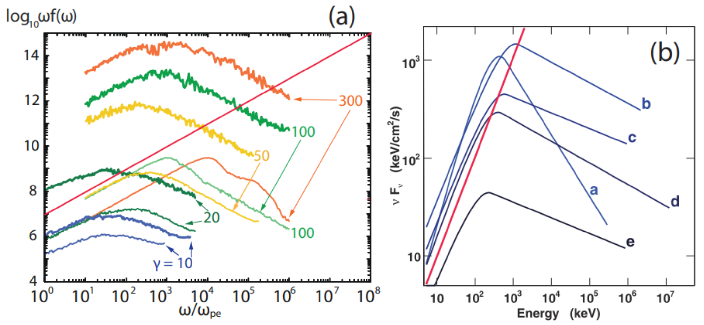
Accelerated electron radiation spectra were self-consistently calculated, and it was noticed that the spectra depend on the temperature and the initial Lorentz factor of the jet; see Figure 1.

Synthetic spectra calculated self-consistently (i.e., they are collected in situ) were also shown by our earlier work [84], where a comparison of synthetic spectra with the Fermi observations of the GRB 080916C source was given at five different times. Several other works (e.g., [85,86,87]) of synthetic spectra calculations employed a static (or frozen) electric field, although this field was self-consistently obtained in the PIC simulations and the particles were treated as test particles.

The radiation spectra shown in Figure 1 were directly calculated from the simulations by integrating the expression for the retarded power, derived from Lienard–Wiechert potentials (see [81,88]), and were obtained for electron emission from relativistic jets with Lorentz factors $\gamma$ = 10, 20, 50, 100, and 300. These electron spectra (without radiation losses) were calculated for radiation beamed along the jet axis and were attained where a strong magnetic field, WI, and acceleration were strongest in the simulation. A comparison between these synthetic spectra and the spectra of the work of [89] showed a similar trend, indicating that the temporal evolution of the spectrum from early to late times is similar to the synthetic spectra shown here, which are associated with higher to lower jet Lorentz factors.

3.1.2. Shear Velocity Simulations with the Slab Model and Cylindrical Jets

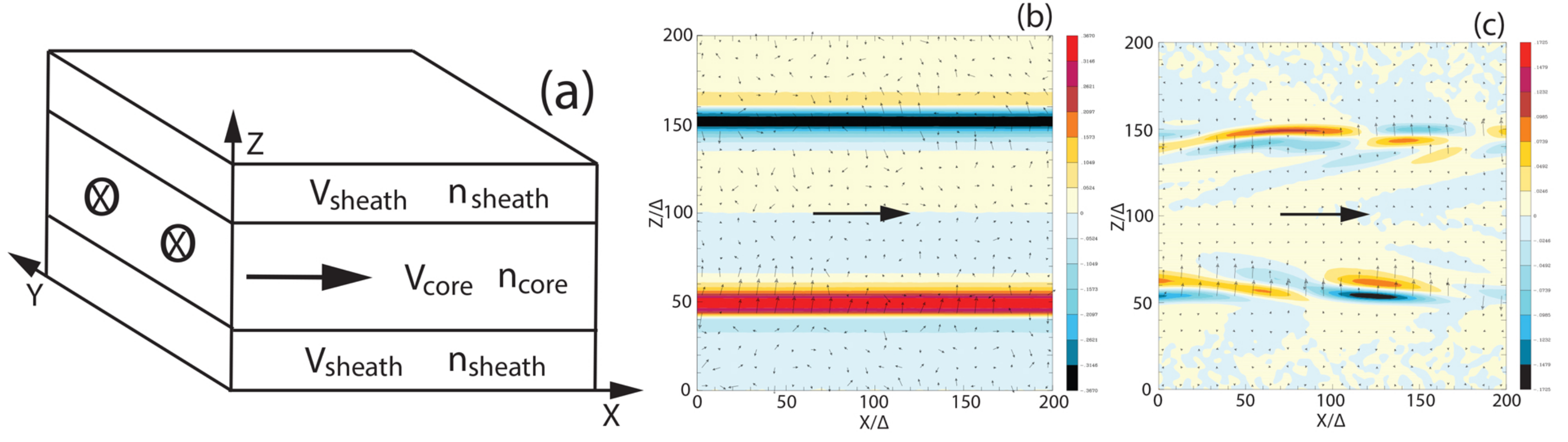
In the same work of [69], the simulation system under investigation used was small, so one cannot fully distinguish shear velocity effects and current filaments associated by the WI or kKHI. Later on in this paper (in Section 3), we discuss an advanced recent work that showed clear differences among different plasma cases, for much larger and more developed plasma jet systems. We investigated the magnetic field generation and development in shear velocities, as these are of importance, applicable to the jets of AGNs and GRBs, since they are expected to present shear velocity phenomena occurring between faster- and slower-moving astrophysical plasmas, both within the jet and at its external medium in-contact interface. In these simulations, a relativistic plasma jet core was applied with a stationary plasma sheath with plasma jet cores of Lorentz factors of 1.5, 5, and 15 for both electron–proton and electron–positron plasmas, as shown in Figure 2 and the description in the legend. In this work, it was found that for the electron–proton plasma, the generation of strong large-scale DC currents and magnetic fields occurred, which extended over the entire shear surface and reached thicknesses of a few tens of electron skin depths. On the other hand, for electron–positron plasma, the generation of alternating AC currents and magnetic fields was found. Some indications given in these simulations showed that kKHI induced jet and sheath plasmas acceleration across the shear surface in the strong magnetic fields. Moreover, the mixing of jet and sheath plasmas showed the generation of a transverse structure similar to that produced by WI.

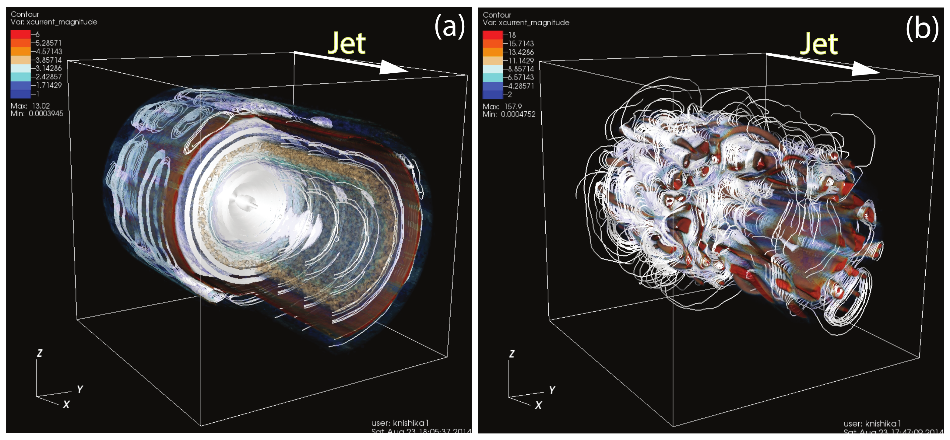
Relativistic jets and internal filamentary structures can be suitably studied via a cylindrical shape. A shear velocity in a jet could cause electromagnetic field structures and instabilities, which can be studied by PIC simulations. In particular, a shear velocity in cylindrical geometry for a $e^{-}-p^{+}$ and an $e^{\pm }$ jet was investigated in [69] for a relativistic jet of $\gamma =15$. In Figure 3, one sees the isocontour displays of the x component of the current $J_x$ along with the magnetic field lines (one-fifth of the jet size), Plot (a) for an $e^{-}-p^{+}$ and Plot (b) for an $e^{\pm }$ jet at a simulation time $t=300{\omega }_{pe}^{-1}$. The magnetic field lines are generated by kKHI. Upon close inspection, one understands that in the $e^{-}-p^{+}$ jet, the currents are generated in thin layers, and the magnetic field is wrapped around the jet. On the contrary, for the $e^{\pm }$ jet case near the shear velocity, well-defined current filaments are induced, which are wrapped by the magnetic field. These characteristic differences may be very useful for observational astronomy by means of circular and linear polarization, as we also discuss later.

In [69], we also showed the development of the MI mode at the earlier linear stage, even when we had not yet identified it explicitly as MI! At the nonlinear stage, the wavelength of MI became very large, resulting in a DC magnetic field, as also shown in another similar work [90]. For relativistic jets with a higher Lorentz factor, MI became dominant compared to the kKHI observed in the work [66]. It seemed likely that MI is the source of the DC magnetic field. By inspecting further Figure 3 (adapted from [69], it seemed that the $e^{\pm }$ jet manifested many distinct current filaments near the shear velocity as the individual current filaments are wrapped by the magnetic field, which clearly indicated MI.

3.1.3. Global Simulations of Unmagnetized Relativistic Jets

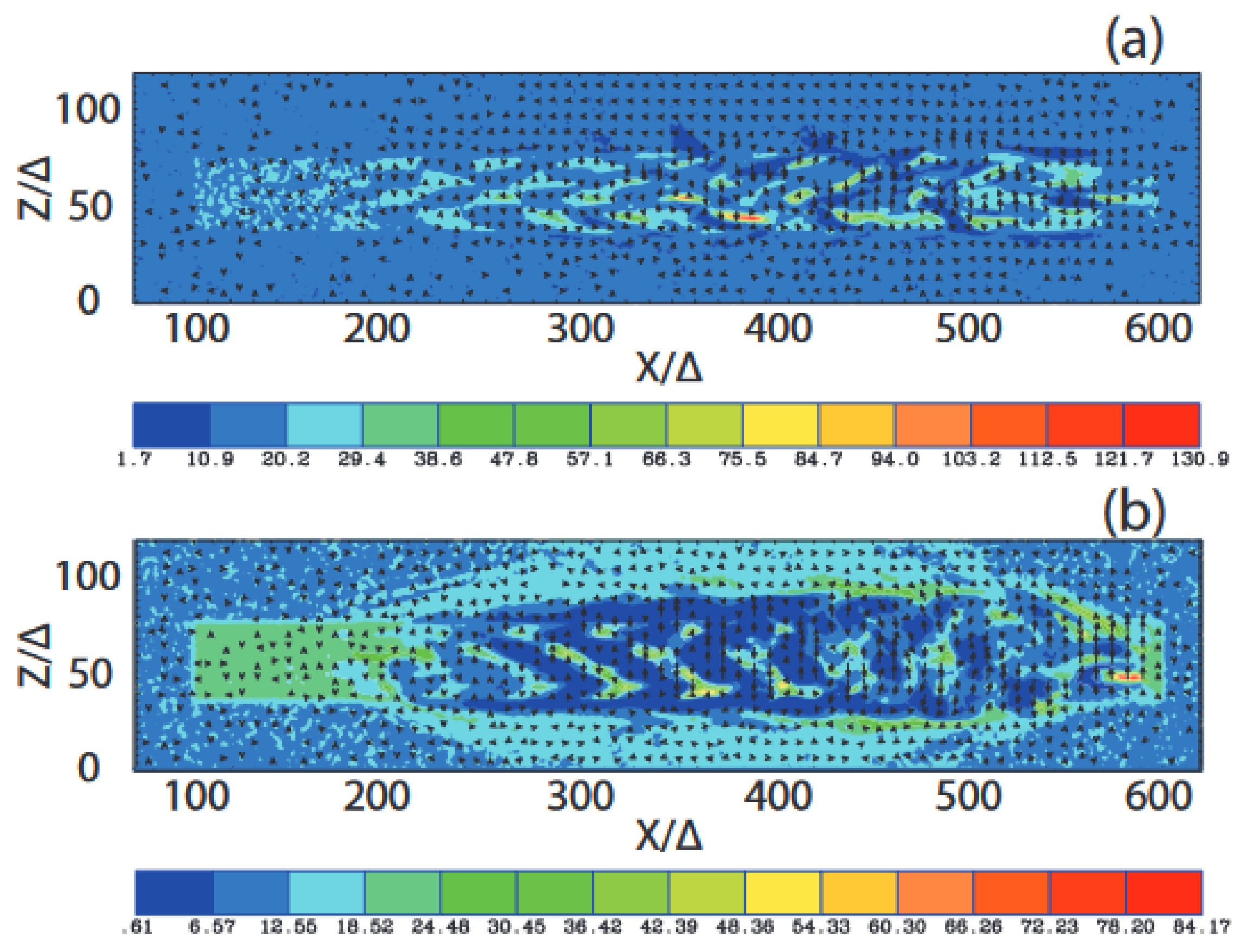
Our simulations of [69] were some of the first ones to lead to the investigation of global jets involving the injection of a cylindrical jet into an ambient plasma, so as to concurrently investigate shock (WI) and shear velocity (kKHI) instabilities. In a relatively small system, nevertheless, as previously mentioned, we also examined any fundamental differences between different jet compositions. In Figure 4, 2D midplane slices of the electron density and the transverse magnetic field are indicated, and one sees how the fast current-driven instability in the shock precursor excites current filaments for the different cases (Panels a and b) at the jet front, as also similarly shown by the work [91]. It is evident that by comparing the electron–proton and electron–positron jets, significant electron density structure differences are noted. In the electron–positron case, electrons and positrons are found outside the jet periphery because positrons are less heavy and mobile than protons, while in the electron–proton jet, electrons and protons remain within the jet rim. This behavior is due to the differently growing WI in different jet compositions, with its associated current filaments, as shown in an earlier work [92].

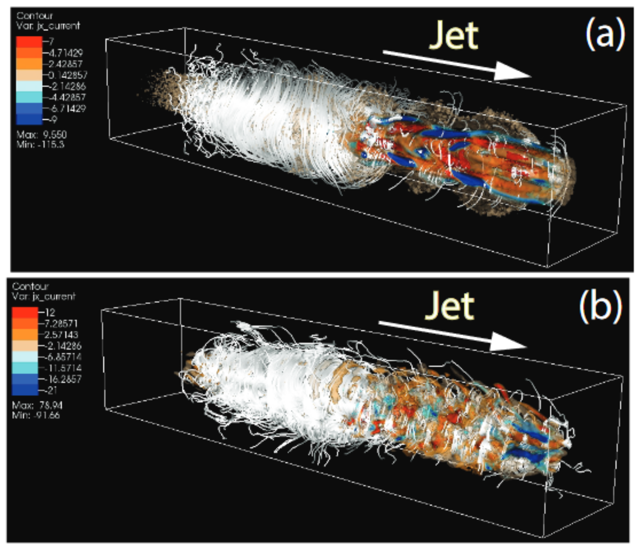
In Figure 5, one sees snipped 3D images taken for $e^{-}-p^{+}$ (a) and $e^{\pm }$ (b) jets at time $t=500{\omega }_{pe}^{-1}$ at $x/\Delta =320$ and $y/\Delta =66$ (adapted from [69]). The jet is propagating from left to right. In these cross-sections, one sees the current filament isosurfaces along with the magnetic field lines that are generated by WI (and kKHI). Upon close inspection, one sees that for both jet cases, in general, compact current filaments are confined mostly within the jet and the current filaments are wrapped by the magnetic field lines. In detail, uninterrupted, long current filaments for the $e^{-}-p^{+}$ jet case are confined within the jet and along the shear velocity surface behind the jet front (Panel a), while in the $e^{\pm }$ jet case, some short current filaments lie outside the jet along the shear velocity surface behind the jet front (Panel b). The pattern of current filaments lying inside and outside of the jet for the $e^{\pm }$ jet at smaller Lorentz factors was also observed in a slab geometry jet in an earlier work [92].

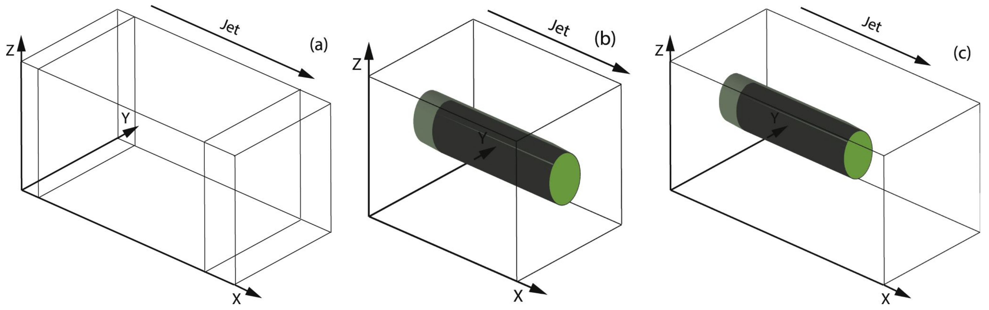
Later on, in a similar simulation [17], the initial evolution for both electron–proton ($e^{-}-p^{+}$) and electron–positron ($e^{\pm }$) relativistic jets was followed, with 3D PIC simulations in a global approach. The jet radius was five-times larger ($r_{jt}=100\Delta$) than the jet radius used in the study [68] with a Lorentz factor ${\gamma }_{jt}=15$ and a suitably larger computation system, with ($L_x,L_y,L_z$) = ($2005\Delta ,1005\Delta ,1005\Delta$). The jet and ambient (electron) plasma number density measured in the simulation frame was $n_{jt}=8$ and $n_{am}=11.1$, respectively. The electron skin depth in the ambient medium was ${\lambda }_s=10.4\Delta$, and the electron Debye length for the ambient electrons ${\lambda }_{=}1.2\Delta$. The ambient plasma at rest was $v_{am}=0$. The simulation was followed until time $t=1700{\omega }_{pe}^{-1}$. The electron jet thermal velocity $v_{jt,th,e}=0.014c$ in the jet reference frame. The electron thermal velocity in the ambient plasma was set to $v_{am,th,e}=v_{am,th,p}=0.05c$, and the ion thermal velocities were smaller by ($m_i/m_e{)}^{1/2}$. The simulations involved a cylindrical jet injection into an ambient plasma, without a magnetic field. For comparison purposes, see Figure 6 and the description in the figure legend about the different approaches (a, b, c) of the geometrical simulation setups for shock simulations in the transverse direction, cylindrical jet injection, and global jet injection.

The aim of these simulations [17] was to investigate shocks (i.e., WI) and shear velocity instabilities (kKHI and MI) simultaneously, since in [69], WI and the shear velocity instabilities were studied separately. A detailed theoretical description of the kKHI and MI growth rates can be found in the same work [17].

In this work, we focused on the jet’s lateral interaction with the ambient plasma. kKHI and MI were found to generate toroidal magnetic fields. The induced magnetic field collimated the jet for the electron–proton jet, and the electrons were perpendicularly accelerated. Meanwhile, as the jet evolved and the instabilities weakened and saturated, the polarity of the magnetic field switched from the clockwise to the counterclockwise direction in the middle of the jet. On the other had, strong mixing of electrons and positrons with the ambient plasma was found in the electron–positron jet case, subsequently resulting in a bow shock formation. Interestingly, a forward shock formed as well during the merging of current filaments, and consequent density inhomogeneities were established. The strong plasma mixing of the ambient plasma with the jet gave also hints of a jet collimation and particle acceleration at the bow shock.

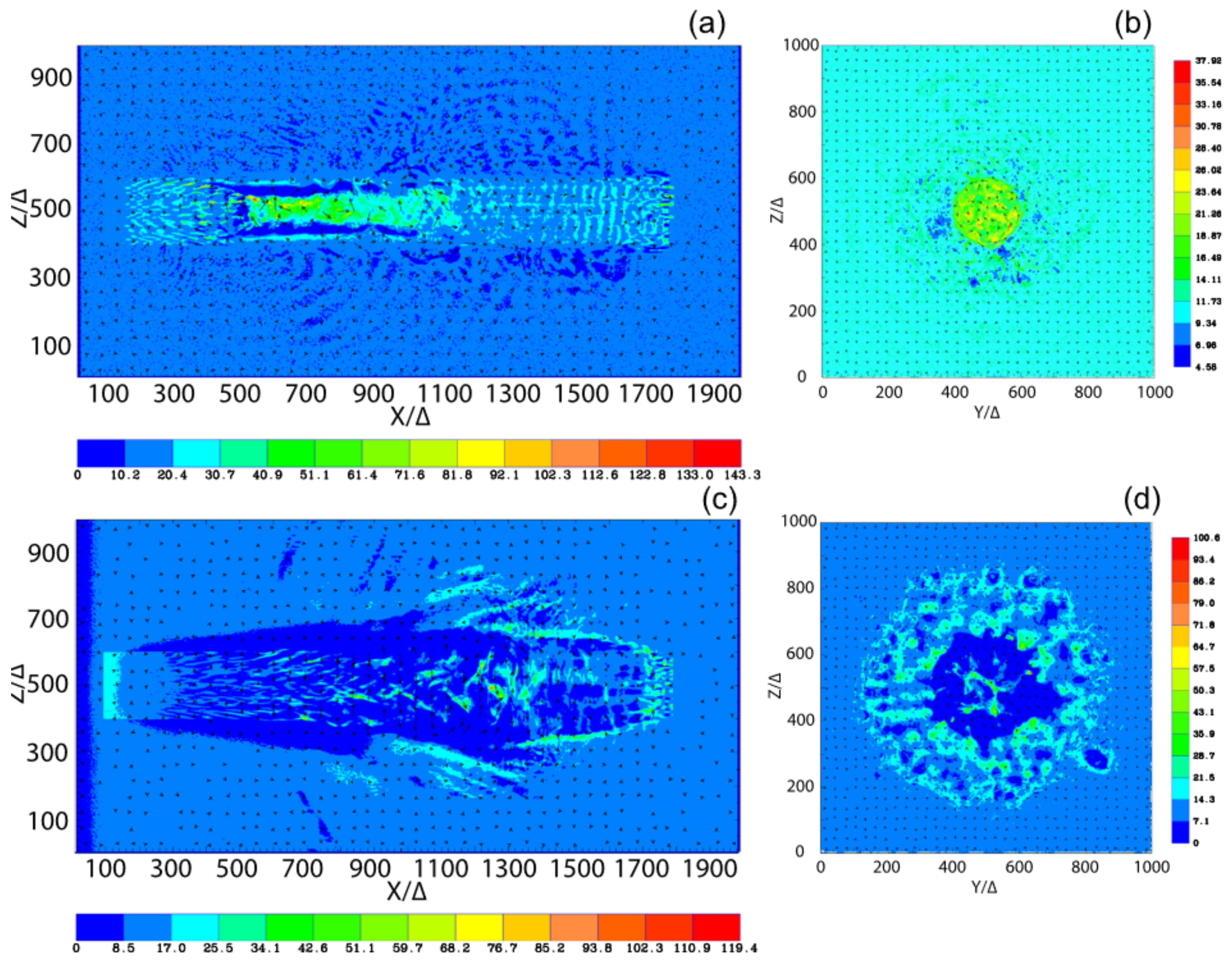
In Figure 7, one sees the global evolution of relativistic electron–positron and electron–proton plasma jet where one can deduct useful conclusions. Collimation takes place for the electron–proton case, at $500\Delta <x<750\Delta$, because kKHI and MI generate the toroidal magnetic fields. Moreover, jet electrons are pinched toward the center where current filaments merge and create a high electron density at $x\sim 500\Delta$. Beyond $x\sim 1000\Delta$, the collimation gradually dissipates. The jet protons, being heavy, define the jet. The wavy patterns, which are intrigued by MI and kKHI, extend for $r\ll r_{jt}$ (Panels a and b). On the contrary, we see that for the electron–positron jet, there is a mixing of light jet electrons and positrons with ambient particles at the shear velocity boundary, as also was shown in the earlier studies [68,69] for the cylindrical core sheath scheme. WI, as shown in earlier work [22], is excited in the jet, and density fluctuation patterns are generated around $x=1250\Delta$. Meanwhile, the jet and ambient electrons move away from the jet boundary due to the MI and kKHI excitation in the shear velocity region (see Panels c and d of Figure 7).

The simulations of [67] revealed that the combined processes and instabilities develop very differently for electron–proton and electron–positron jets. The key simulation results are summarized as follows, for the $e^{-}-p^{+}$ jet:

1.

Jet electrons are collimated by strong toroidal magnetic fields generated by MI;

2.

Electrons are perpendicularly accelerated along with the jet collimation;

3.

The toroidal magnetic field polarity switches from clockwise to counterclockwise about halfway down the jet.

For the $e^{\pm }$ jet, the key simulation results are:

1.

Jet electrons and positrons mix with the ambient plasma;

2.

Magnetic fields around current filaments generated by a combination of kKHI, MI, and Weibel instability merge and generate density fluctuations;

3.

A larger jet radius is required to properly simulate the $e^{\pm }$ jet case, since the jet and ambient particles mix strongly.

Below, we present even larger spatiotemporal simulations with a helical (Section 3.2.2) and a toroidal (Section 3.2.3) magnetic field, in order to investigate the effect the topology of these magnetic fields has on the growth of plasma instabilities (WI, MI, and kKHI) and on the consequent particle acceleration.

3.2. Magnetized Jets

3.2.1. Topology of Relativistic Helical Jets

Most relativistic jets are collimated and extend between several thousands up to millions of parsecs [1]. These astrophysical jets present highly complex phenomena, which except relativistic plasma speeds, have helical magnetic fields emanating from the central compact source engulfing the plasma outflow. Therefore, in a simulation study, it is natural to inject jets with helical (e.g., toroidal/poloidal) magnetic fields [93].

As shown in relevant PIC simulations [18,20], which we present in Section 3.2.2 and Section 3.2.3 below, the helical magnetic fields are not generated with the jets powered by a self-consistent rotating black hole; therefore, a force-free helical magnetic field is implemented at the jet’s aperture. In [18,67], we used the force-free helical magnetic field topology in the laboratory frame with poloidal ($B_x$) and toroidal ($B_{phi}$) coordinates [62], such as:

$$\begin{array}{c}\hfill B_x=\frac{B_0}{{[1+{(r/\alpha )}^2]}^p},B_{\varphi }=\frac{B_0}{(r/\alpha ){[1+{(r/\alpha )}^2]}^p}\sqrt{\frac{{[1+{(r/\alpha )}^2]}^{2p}-1-2p{(r/\alpha )}^2}{2p-1}}\end{array}$$

(2)

where, r is the radial position in cylindrical coordinates, $B_0$ is the magnetic field (the toroidal field component is a maximum at $\alpha$ for constant magnetic pitch), and p is a pitch profile parameter. The PIC simulations were performed in Cartesian coordinates, and the characteristic length scale $p=1$, so Equation (2) reduces to,

$$\begin{array}{c}\hfill B_x=\frac{B_0}{[1+{(r/\alpha )}^2]},B_{\varphi }=-\frac{(r/\alpha )B_0}{[1+{(r/\alpha )}^2]}.\end{array}$$

(3)

The current $+J_x(y,z)$ creates the toroidal magnetic field (the poloidal field component, $B_x$, is not included), and it is in the positive x-direction. In Cartesian coordinates then, the y- and z-coordinate of the magnetic field is,

$$\begin{array}{c}\hfill B_y(y,z)=\frac{(z-z_{\mathrm{jc}})B_0}{\alpha [1+{(r/\alpha )}^2]},B_z(y,z)=-\frac{(y-y_{\mathrm{jc}})B_0}{\alpha [1+{(r/\alpha )}^2]}.\end{array}$$

(4)

The characteristic length-scale of the helical magnetic field is $\alpha$, and the center of the jet is given by ($y_{jc},z_{jc}$), such as,

$$\begin{array}{c}\hfill r=\sqrt{{(y-y_{jc})}^2+{(z-z_{jc})}^2}\end{array}$$

(5)

The above Equation (5) defines the chosen helicity of the magnetic field, which has a left-handed polarity with a positive $B_0$. The helical magnetic field is implemented without the motional electric field at the jet aperture. This corresponds to a self-consistently generated toroidal magnetic field by jet particles moving along the $+x$-direction.

In the simulations of [20], an $\alpha =4$ was used, which due to the narrow current generating the toroidal magnetic field, an excitation of a kinetic current -driven instability was found to be developing before the growth of MI and kKHI. For that reason, in our most recent work [15], a new injection scheme was adopted to avoid this fact, while using small $\alpha =2$, MI and kKHI grow faster than the current-driven instability. The jet particles for both these studies (presented below) are injected at $x=100\Delta$, and they propagate as shown by the cylindrical shape in Figure 8. The components of the helical fields, i.e., the poloidal field represented by $B_x$ (black) and the toroidal field $B_{\varphi }$ (red), are depicted with different pitch profiles. We can see that the toroidal magnetic fields become zero at the center of the jet (red lines). If the pitch profile parameter is $0.5<\alpha <1$, then the magnetic pitch increases with the radius, and if $\alpha >1$, then the magnetic pitch decreases. Figure 8b shows different values of $\alpha$ for comparative reasons. In [18], for the PIC simulations (see the next subsection), a constant pitch $\alpha =1$ was used with a jet radius $r_{jt}=20,40,80$, and $120\Delta$. Here, b is the dumping factor of the magnetic fields outside the jet. It is noted that these global jet simulations were performed with the simplest type of jet structure, that is a top-hat shape (flat density profile).

3.2.2. Global Simulations with Helical Jets and Large Radii

In the work [18], we used smaller simulations within a numerical grid ($L_x,L_y,L_z$) = ($645\Delta ,131\Delta ,131\Delta$) where the simulation cell size was $\Delta =1$ and examined the helical magnetic effects on a jet’s evolution. In these simulations, the electron skin depth was $\lambda =c/{\omega }_{pe}=10.0\Delta$ and the electron Debye length for the ambient electrons was ${\lambda }_D=0.5\Delta$, where c is the speed of light and ${\omega }_{pe}$ is the electron plasma frequency.

It was indicated that although the simulation system was short, the growing instabilities were affected by the helical magnetic fields of the electron–proton and electron–positron jets. Complicated patterns of $B_y$ were produced by the currents, which were generated by instabilities. Interestingly, it was found that a larger jet radius contributed to the growth of more instability modes, making the jet structures more complicated. Longer simulations, discussed below, gave us even more information of the instabilities’ development and the propagation of jets with helical magnetic fields. Regarding particle acceleration, it was interestingly shown that the changing directions of the local magnetic fields, being generated by the instabilities, coincided with the patterns of the Lorentz factor of the jet particles.

In [20], new 3D PIC simulations were performed with a larger numerical grid size ($L_x,L_y,L_z$) = ($1285\Delta ,789\Delta ,789\Delta$) in Cartesian coordinates. In this simulation, the longitudinal box size $L_x$ and the simulation time $t_{max}=1000{\omega }_{pe}^{-1}$ were a factor of two larger than the previous simulations of [18,19,67], with radii $r_{jt}=20,40,80,120\Delta$. Open boundaries at $x/\Delta =0$ and $x/\Delta =1285$ and periodic boundary conditions in the transverse directions were applied. The jet was injected at $x=100\Delta$ in the center of the y-z plane. Its radius $r_{jt}=100\Delta$. Since a large computational box was applied, this allowed following the jet’s evolution long enough to examine also the nonlinear stage of the system. The jet head had a flat-density top-hat shape. This topology is only a simplified approach of a true jet-formation structure region (e.g., [94]). A more realistic jet structure with, e.g., a Gaussian-shaped head is the aim of our future work. Although as shown in [17,18,19], jets of different plasma composition exhibit distinct dynamical behavior that manifests itself in the morphology of the jet and its emission characteristics, only the case of an electron–proton jet with a helical magnetic field was investigated in this work.

These simulations focused on the interaction between the jet and the ambient plasma, as we wanted to explore how the helical magnetic field affects the excitation of kinetic instabilities such as WI, kKHI, and MI. It was found that these kinetic instabilities were indeed excited, as expected, and particles were also accelerated. At the linear stage, recollimation shocks were observed near the center of the jet, and as the electron–proton jet evolved into the deep nonlinear stage, the helical magnetic field became untangled due to reconnection-like phenomena. It was consequently found that electrons were repeatedly accelerated at the magnetic reconnection regions within the turbulent magnetic field. Comparatively, similar works [95,96,97] presented theoretically and numerically the particle acceleration process in turbulent reconnection. An exponential growth in the energy of the accelerated particles was demonstrated along with a power law tail development in the outcome particle spectrum. These are signatures of stochastic Fermi acceleration, by reconnection. In Figure 5 of [20], a power law tail was shown, which is consistent with the similar above-mentioned studies; nevertheless, future studies are needed to confirm the stochastic Fermi acceleration nature of this result.

The similar PIC simulation work [64] showed that in kink-unstable jets, curvature drift accelerates particles, during the formation of highly tangled magnetic fields and a large-scale inductive electric field. In their simulations, there was no bulk flow; therefore, velocity shear instabilities such as kKHI and MI were not excited, and KI occurred instead. The magnetization in their simulations was very large, i.e., $\sigma >1$, where $\sigma =B^2/n_e{m}_e{\gamma }_{jt}{c}^2$, so the toroidal magnetic field was dominant and KI was triggered, consequently tangling the helical magnetic field and probably resulting in acceleration via reconnection, not only necessarily via a curvature drift mechanism. Our simulations [20] did not show a kink-like instability as the simulations of [98] showed, since MI and kKHI grew faster than the current-driven kink instabilities due to the strong shear velocity and the moderate magnetization of the jet.

As was described in the previous subsection, a cylindrical jet containing a helical magnetic field was applied in [20], propagating in the x-direction, injected into an ambient electron–proton plasma at rest, as shown in Figure 8 and described by Equations (2)–(5). The initial particle number per cell was $n_{jt}=8$ and $n_{am}=12$, respectively, for the jet and ambient plasma. The electron skin depth was ${\lambda }_s=c/{\omega }_{pe}=10.0\Delta$, where c is the speed of light and ${\omega }_{pe}={(e^2{n}_{am}/{ϵ}_0{m}_e)}^{1/2}$ is the electron plasma frequency, and the electron Debye length of ambient electrons is ${\lambda }_{\Delta }=0.5\Delta$. Moreover, the thermal speed of jet electrons was set to $v_{jt,th,e}=0.014c$ in the jet reference frame, while in the ambient plasma, it was $v_{am,th,e}=0.03c$. A temperature equilibration was assumed, so the thermal speed of the ions was smaller than that of the electrons by a factor of ${(m_p/m_e)}^{1/2}$. A realistic mass ratio of $m_p/m_e=1836$ was also applied. The jet Lorentz factor was ${\gamma }_{jt}=15$. The jet plasma was initially weakly magnetized, and the magnetic field amplitude parameter $B_0=0.1c$ corresponded to a plasma magnetization $\sigma =B^2/n_e{m}_e{\gamma }_{jt}{c}^2=2.8\times {10}^{-3}$.

The particles were found to be accelerated by a turbulent magnetic reconnection effect, shown in Figures 1a,b and 4 of [20], initiated by the growth of kinetic instabilities such as kKHI and MI, the most dominant of which was MI, which pinched the jet and generated recollimation shocks. In our simulation analysis here, it appears that, first, kKHI and MI (WI) grow, then recollimation shocks form, and later, reconnection operates. The recollimation shocks feature a quasi-static electric field, $E_x$, which depending on its sign, accelerates or decelerates the jet electrons. We add that kKHI contributes to the recollimation shocks formation. The tracer magnetic field reversals and other diagnostics we applied found regions in which magnetic reconnection occurred, which was discussed further in [15] and in Section 3.2.3 below. Note that it was also observed that a strong transverse magnetic field $B_y$ coincided with the produced parallel electric field $E_x$. Interestingly, this kind of behavioral trend showed similarities to the structure of recollimation shocks in the RMHD simulations of [62].

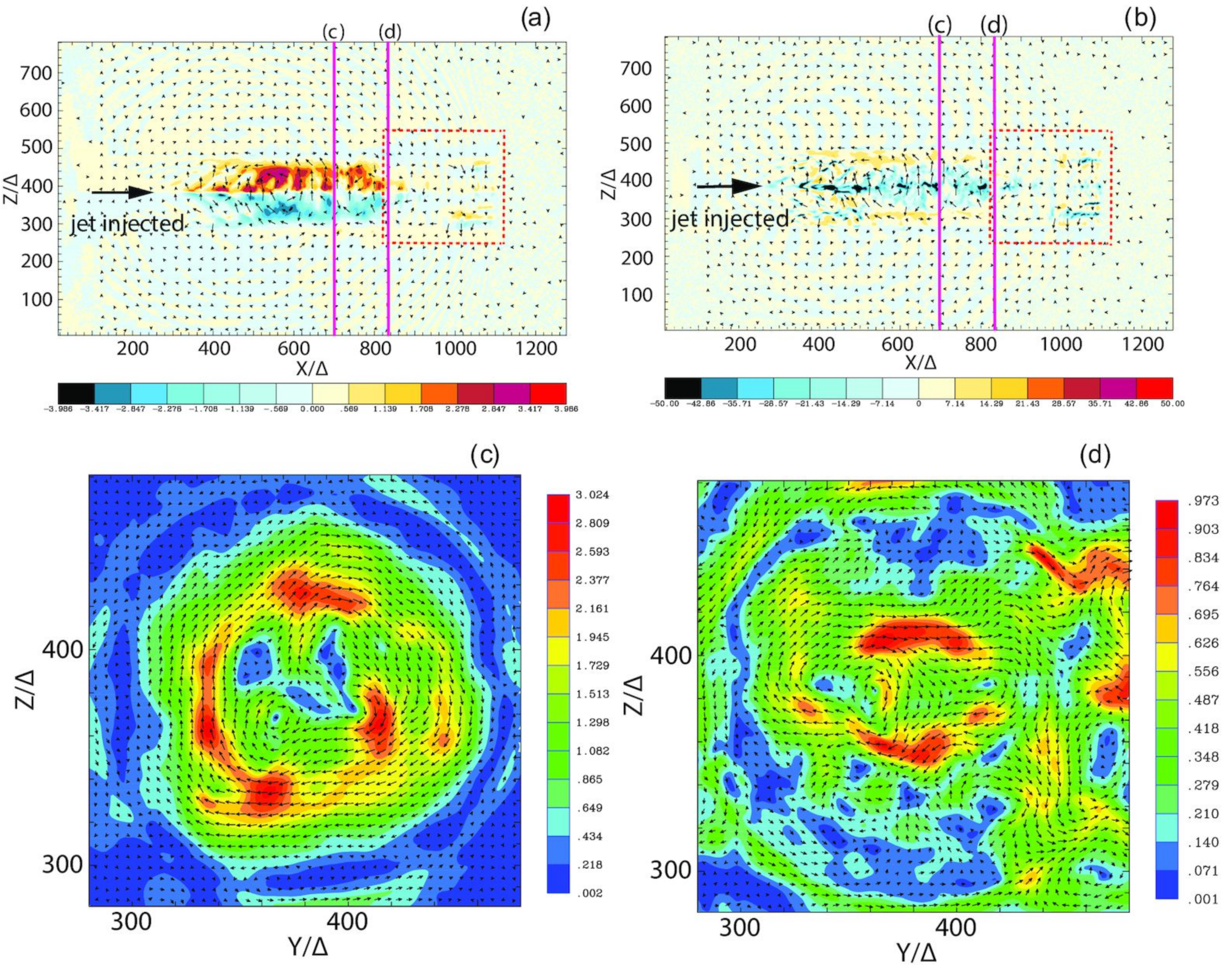
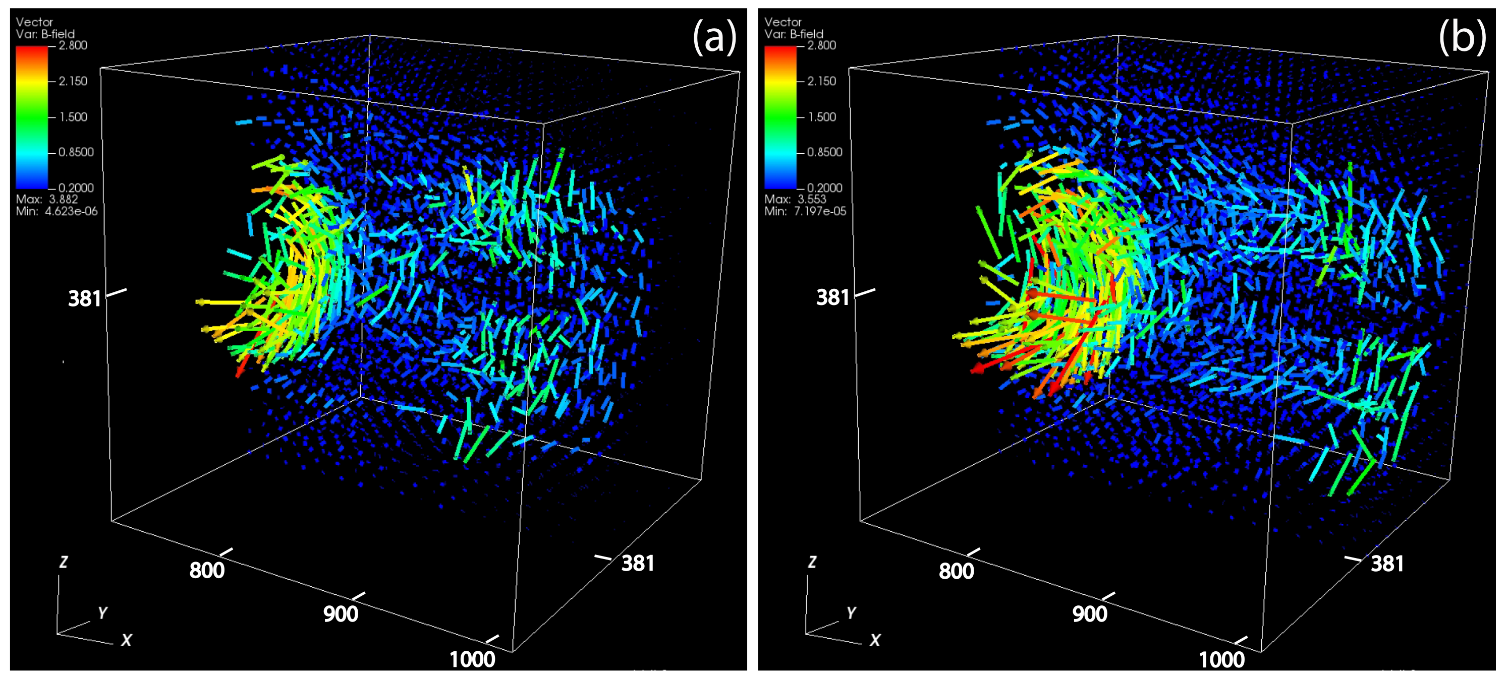
As the simulation progressed to the nonlinear stage, the toroidal magnetic fields were found to become untangled, as Figure 9 shows, where cross-sections are indicated through the center of the jet at time $t=1000{\omega }_{pe}^{-1}$. The jet propagates from the left to right. The figure shows the y-component (a) of the magnetic field, $B_y$, with the x-z electric field as arrows, and (b) the x-component of the electron current density, $J_x$, with the x-z magnetic field depicted as arrows. At $400\le x/\Delta \le 830$, a strong helical magnetic field in the jet can be discerned. As shown in Figure 9a, the amplitude with $B/B_0\approx 40$ is much larger than that of the initial field. As discussed above and in an earlier work [17], this field results from the grown instabilities (MI and kKHI). However, in the presence of an initial helical magnetic field, the growth rate of the transverse MI mode is reduced. The field structure is strongly modulated by longitudinal kKHI wave modes as shown by the bunched $B_y$ field (Figure 9a). The above phenomena cause multiple collimations along the jet, which are caused by the pinching of the jet electrons toward the center of the jet, as is visible in the electron current density (Figure 9b). In the same Panel (b), we can discern that $B_y$ is weak exactly where the collimations become weaker along the jet, disappearing at around $x/\Delta \ge 830$. This fact makes evident that the MI nonlinear saturation actuates the dissipation of the helical magnetic field. A similar behavior was observed in the recent work [15], which we discuss below.

Moreover, in Figure 9a,b, possible reconnection sites are shown by the two red lines at $x/\Delta =700$ and $x/\Delta =835$. In Figure 9c,d, the magnetic field structure is shown “head-on”, i.e., in the y-z plane. By inspecting the configuration of the field, one discerns that at $x/\Delta =700$, a clockwise circular magnetic field is split near the jet into a number of magnetic structures, which indicate the growth of MI. These structures are surrounded by a field of opposite polarity that is produced by the proton current framing the jet boundary (see also [15,17]. At $x=835\Delta$, the magnetic field is strongly turbulent. The helical structure is distorted and is reorganized into multiple magnetic islands, which reveal the nonlinear stage of MI and kKHI. Accordingly, we see that the magnetic islands interact with each other, providing conditions for magnetic reconnection. We should note at this point that in a 3D topology, a reconnection site does not occur at a simple X-point as in a 2D slab geometry. Instead, reconnection sites can be identified by regions of weak magnetic fields surrounded by oppositely directed magnetic field lines. An example of a possible site of reconnection can be discerned at ($y/\Delta /,z/\Delta$) = ($380,340$). In that region, the total magnetic field has a so-called null point (becomes minimal); see Figure 9d.

The 3D topology of the jet’s magnetic field is shown in Figure 10. The magnetic field vectors are indicated at $t=900{\omega }_{pe}^{-1}$ (Figure 10a) and $t=1000{\omega }_{pe}^{-1}$ (Figure 10b). The red dashed rectangle in Figure 9b is the respective region indicated at $820<x/\Delta <1120;231<y/\Delta ,z/\Delta <531$) in Figure 10b. The image is snipped at the center of the jet at $y/\Delta =381$. One can discern that the rim of the helical magnetic field in the jet moves slower than the jet speed. In particular, the edge of the helical magnetic field moves from $x/\Delta =780$ at $t=9000{\omega }_{pe}^{-1}$ to $x/\Delta =830$ at $t=1000{\omega }_{pe}^{-1}$, while with the same jet speed, the front should be at time $t=1000{\omega }_{pe}^{-1}$ placed at $x/\Delta =880$.

This suggests that the frontal rim of the helical magnetic field is decorticated as the jet propagates. Consequently, this may indicate that the helical magnetic field is braided by kinetic instabilities and subsequently becomes untangled, as discussed in [99]. It follows that the untangling of the helical magnetic field results from magnetic reconnection-like phenomena, which push the helical magnetic field away from the center of the jet, at the forward position.

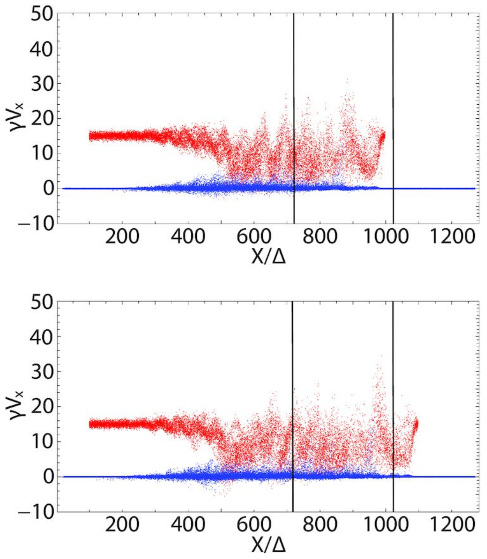
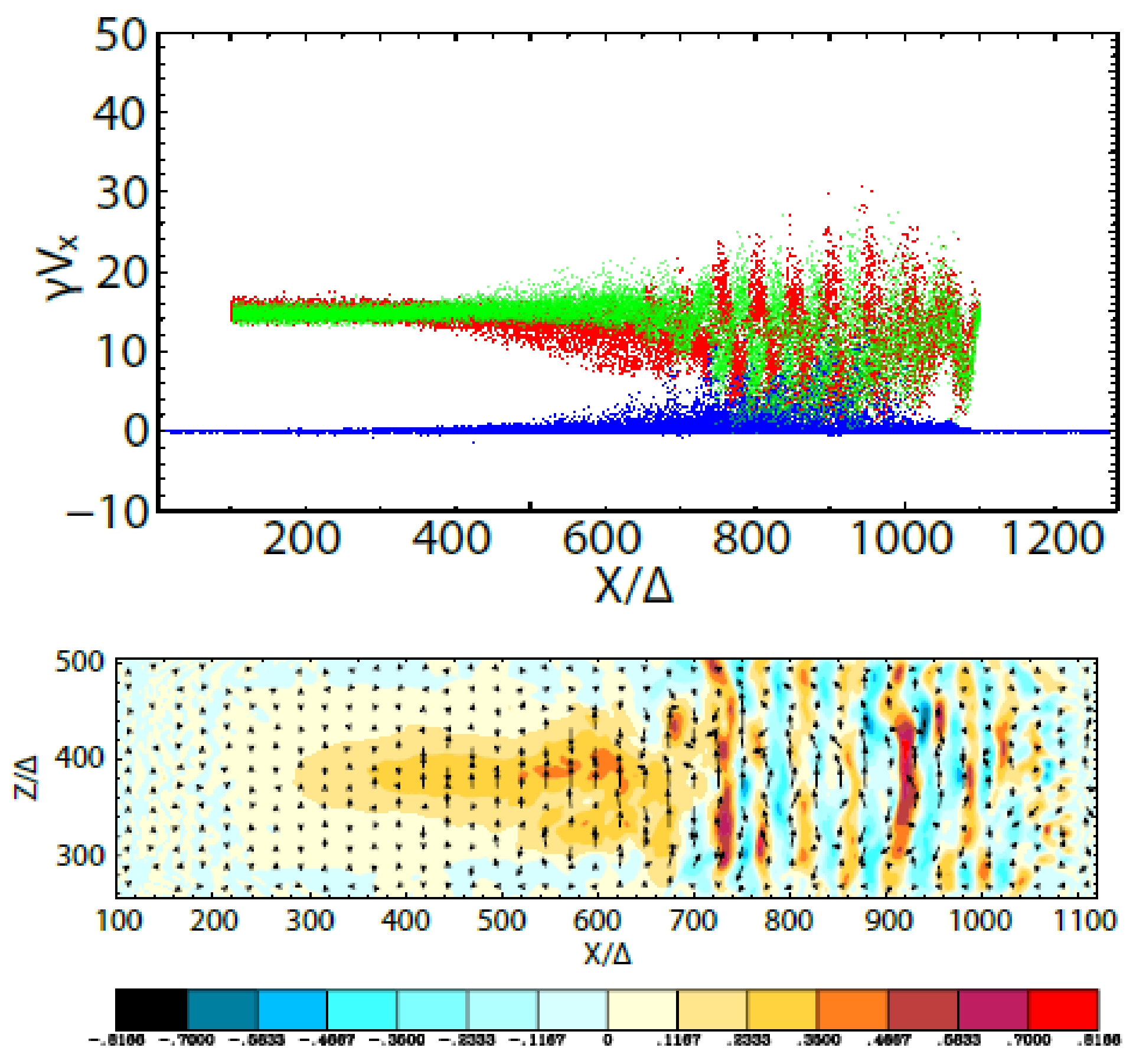
Finally, Figure 11 shows the phase space distribution of jet electrons (red) and ambient electrons (blue) at time $t=900{\omega }_{pe}^{-1}$ and at $t=1000{\omega }_{pe}^{-1}$. The electrons are accelerated at $x/\Delta =780$, where the helical magnetic field disappears, as shown accordingly in Figure 10a. Near $x=830\Delta$, the disappearance of the helical magnetic field also coincides with the acceleration of electrons, and the ambient electrons entrained into the jet plasma are also strongly accelerated.

3.2.3. Global Jet Simulations with a Toroidal Magnetic Field and a New Injection Scheme

In the simulations of [15], we used 3D PIC simulations to study the spatiotemporal evolution of magnetized relativistic electron–positron and electron–proton jets, by comparing magnetized (with toroidal fields) and unmagnetized jets, while focusing on investigating the kinetic instabilities and the associated particle acceleration. Note, as discussed in Section 3.2.1, that in this work, a new jet injection scheme was applied by injecting different compositions of $e^{\pm }$ and $e^{-}-p^{+}$ jets, with a comoving toroidal magnetic field, with a top-hat jet density profile and a current that is self-consistently carried by the jet particles, $\mathbf{J}=\nabla \times \mathbf{B}$. A toroidal magnetic field was applied at the jet orifice in order to sustain the current in the jet, as so, a motional electric field was established.

This work addresses the following key questions:

1.

How does a toroidal magnetic field affect the growth of kKHI, MI, and WI within the jet and in the jet–ambient plasma boundary?

2.

How do jets composed of electrons and positrons and jets composed of electrons and protons evolve in the presence of a large-scale toroidal magnetic field?

3.

How and where are particles accelerated in jets with different plasma compositions?

This study involved a much larger jet radius than the previous works [18]. We pinpointed how the dissipation of the magnetic fields generates electric fields that are sufficiently strong to accelerate particles up to Lorentz factors of 35. In these simulations, the jets were weakly magnetized. The ambient medium was unmagnetized, and the simulation time was sufficiently long in order for the nonlinear effects of the jets’ evolution to be included. The grid was set to ($L_x,L_y,L_z)=(1284\Delta ,789\Delta ,789\Delta$), twice as long than what was used in our earlier simulation studies [18,19,67]. The jet was injected at $x=100\Delta$ in the center of the y-z plane at $(y_{\mathrm{jc}},z_{\mathrm{jc}})$ and propagated in the x-direction. Its radial width in cylindrical coordinates was $r_{\mathrm{jet}}=100\Delta$. The jet Lorentz factor was set to ${\gamma }_{\mathrm{jt}}=15$.

In this work, only a toroidal magnetic field was applied, $B_{\varphi }\left(r\right)=B_0(r/a)[1+{(r/a)}^2]$, as also discussed in Section 3.2.1 (Equations (2)–(4)). The poloidal field component, $B_{\mathrm{x}}$ [20], was not included this time. $B_{\varphi }$ had a peak amplitude at $r=a$, where a is the characteristic radius. In Cartesian coordinates, the corresponding field components, $B_{\mathrm{y}}$ and $B_{\mathrm{z}}$, were calculated from Equation (3). For the field outside of the jet, the above equations were multiplied with a damping function, $\Theta (r-r_{\mathrm{jet}})=\frac{r_{\mathrm{jet}}}{r},\mathrm{where}r>r_{\mathrm{jet}}$.

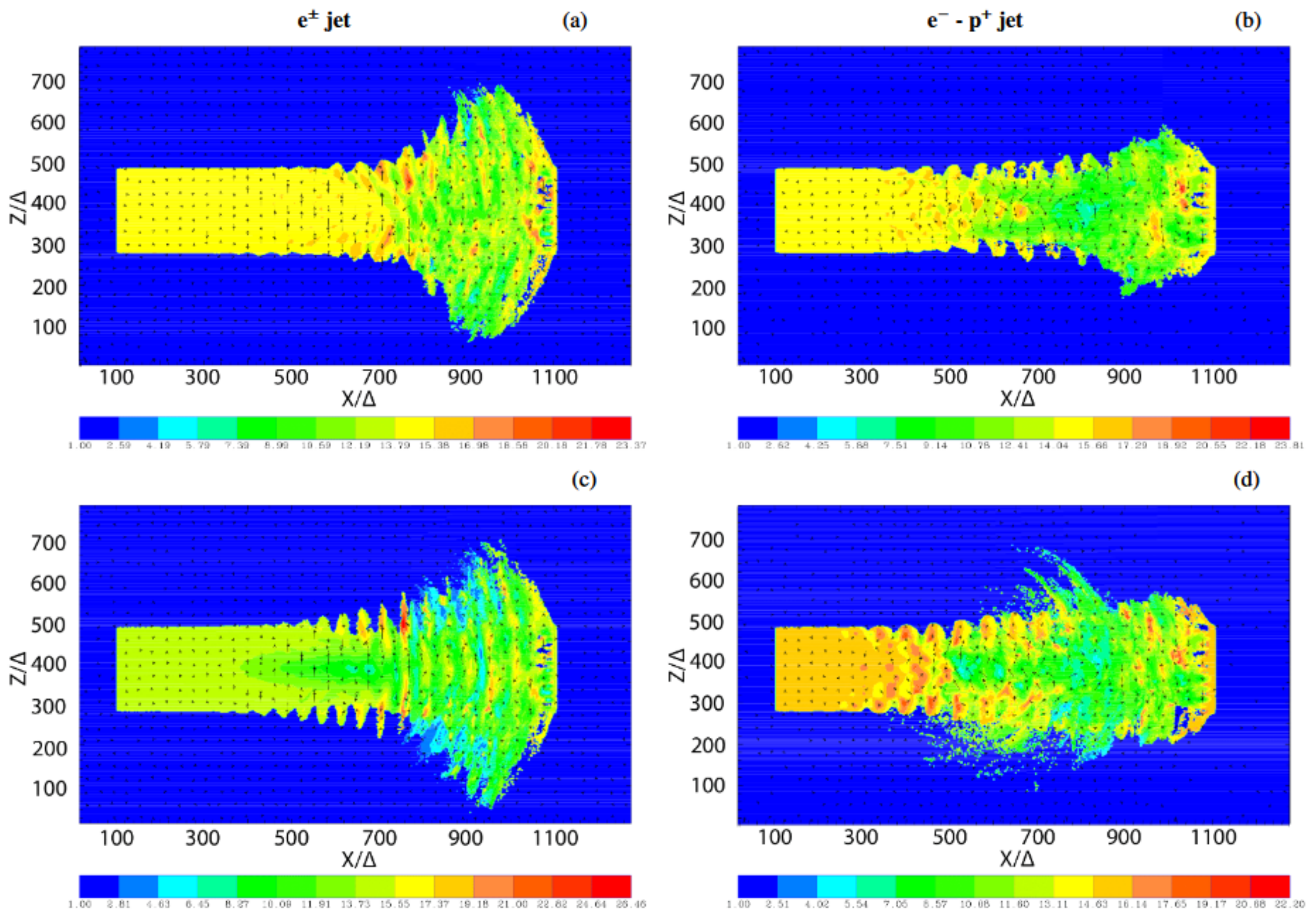
In Figure 12, one sees the global jet structure, while the Lorentz factor is demonstrated for jet electrons for an $e^{\pm }$ (Panels a and c) and an $e^{-}-p^{+}$ (Panels b and d) jet at time $t=1000{\omega }_{pe}^{-1}$. The black arrows in all panels indicate the magnetic field direction in the x-z plane. The structures seen at the boundary, for the $e^{\pm }$ jets, between the jet and the ambient plasma at $500<x/\Delta <1000$ indicate the excitation and development of kKHI and MI. As mentioned in the Introduction, MI represents the transverse component/dynamics of kKHI. In both the unmagnetized and weakly magnetized jets in this work, it is shown that after the dissipation of the magnetic field, around $x/\Delta =800$, the disruption around the jet head is prominent. It is evident that the jets expand radially. This resembles a Mach cone (a bow shock) structure. For the $e^{-}-p^{+}$ jets, the bow shock-like structures are less prominent. A notable difference between the jet with the toroidal magnetic field and the unmagnetized one is that in the first case, the jet electrons are expanded outside the jet at $x/\Delta \simeq 500-900$. That leads to the conclusion that the instabilities excited within the jet, which we discuss more later, push the jet electrons radially.

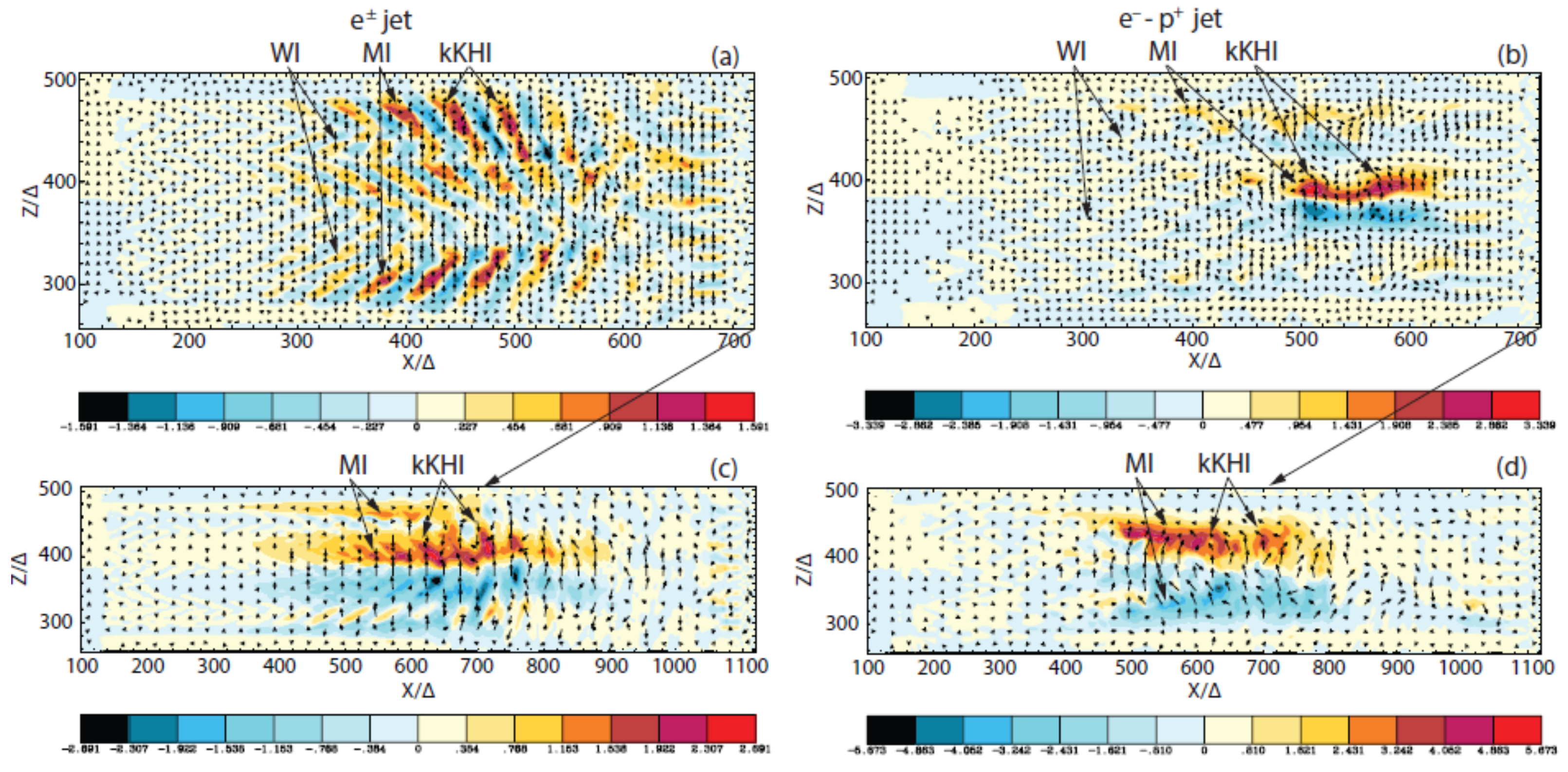
In Figure 13, one sees the magnetic field component $B_{\mathrm{y}}$ in the x-z plane at $y/\Delta =381$ with an in-plane magnetic field depicted with black arrows. The results for jets with toroidal magnetic fields are shown, and the upper panels present the field structures in the linear regime at time $t=600{\omega }_{\mathrm{pe}}^{-1}$, whereas the lower panels depict the nonlinear stage at time $t=1000{\omega }_{\mathrm{pe}}^{-1}$. In the left panels (a, c), an electron–positron jet is shown, and in the right panels (b, d), an $e^{-}-p^{+}$ jet is shown. WI is initially generated within the jet, while at the jet head located at $x/\Delta \approx$ 650–700, this instability generates magnetic field filaments aligned with the jet propagation direction. Downstream along the jet, the oblique mode of WI dominates. This is visible as striped magnetic fields at $x/\Delta \approx$ 300–600, for the $e^{\pm }$ jet (Figure 13a). In the same region of the jet, kKHI and MI start to grow simultaneously, at the jet–ambient medium boundary and across the jet, respectively. The wavelength of WI is about $4{\lambda }_{\mathrm{se}}$. The observed excitation of MI and kKHI is merged with WI. This results in slanted striped structures of the magnetic field in the electron–positron jet. The wavelength of the kKHI mode is about $6{\lambda }_{\mathrm{se}}$, and the wavelength of the MI mode is about $5{\lambda }_{\mathrm{se}}$ along the jet radius, or else perpendicular to the jet axis. Since the growth rates of MI and kKHI are similar, the excited modes propagate towards the jet center. Figure 13c shows the growth of kKHI and MI in the nonlinear stage. MI grows stronger and generates two dominant modes along the jet radius, the inner mode having a larger amplitude. Concurrently, along the jet, the longitudinal kKHI wave modes modulate the magnetic field.

Additionally, Figure 13b, for the $e^{-}-p^{+}$ jet in the linear stage, shows that MI grows around $x/\Delta =400$ dominantly. It then propagates toward the jet center and generates two MI modes. For the nonlinear stage, Figure 13d shows a very strong toroidal (helical) magnetic field in the jet at $t=1000{\omega }_{\mathrm{pe}}^{-1}$ (at approximately $500\lesssim x/\Delta \lesssim 830$), with the amplitude $B/B_0\approx 56$ (see above). The magnetic field amplification seen is attributed to kKHI and MI, which was similarly observed in the unmagnetized case of [17]. Let us note that the outer MI mode merges with the inner mode (Figure 13d).

The same panel (d) shows the growth of kKHI along the jet since the field structure is pinched by MI, which is strongly modulated. This fact demonstrates that the observed field collimation is caused by the pinching of the jet electrons towards the center of the jet, as already noted for the electron density structures in the same work. Figure 13b indicates the detailed structure of the growing modes of both MI and kKHI.

Figure 14 shows the x - $\gamma v_{\mathrm{x}}$ distribution of jet electrons (red), jet positrons (green), and ambient (blue) electrons for a jet pair at $t=1000{\omega }_{\mathrm{pe}}^{-1}$. The color map depicts $E_{\mathrm{x}}$ in the x-z plane at $y/\Delta =381$. The $B_{\mathrm{x},\mathrm{z}}$ field is indicated by the arrows. The slight dislocations of the jet electrons and positrons are the response to the magnetic field structures, as the corresponding variations in $v_z$ found, and they generate through $\dot{\mathbf{E}}\propto \mathbf{j}$ the strips of the positive and negative $E_{\mathrm{x}}$. Inspecting the bottom panel of Figure 14, one sees strong striped patterns of $E_{\mathrm{x}}$, which are generated by the out-of-phase distributions of jet electrons and positrons (top panel).

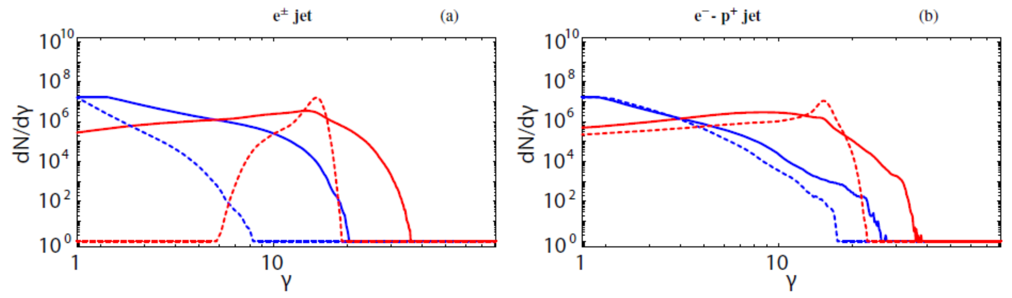
In Figure 15, the energy distribution of the jet (red) and ambient (blue) electrons in and around the $e^{\pm }$ and $e^{-}-p^{+}$ jets in the two regions $x/\Delta <600$ and $x/\Delta >600$ is shown. One sees that the electron acceleration is most significant in the nonlinear stage at the region $x/\Delta >600$. In the linear stage, the ambient electrons are not accelerated as significantly for the electron–positron jet as they are around the $e^{-}-p^{+}$jet. In our work [15], here, we further compared the results and found that the electrons are further accelerated by the disappearance/dissipation of the magnetic fields in the nonlinear stage, a fact that is also seen in the kinetic simulations of the driven magnetized turbulence of [100]. Let us note that in the latter simulation studies, the turbulent magnetic fluctuations were externally forced into the simulation system, and therefore were not self-consistent. Moreover, another work [101] investigated particle acceleration at reconnecting current sheets due to stochastic interactions with turbulent fluctuations (plasmoids and vertexes). In our current simulations [15], plasmoids (vertexes) were generated at the nonlinear stage, and these were shown to accelerate the jet electrons in a similar way. On the contrary, the turbulent magnetic field—where we report multiple magnetic flux ropes—was self-consistently created in the relativistic jets, through the self-consistent disappearance/dissipation of the toroidal magnetic field. For more details, the reader is referred to similar past studies [95,96,97], where they also discussed the particle acceleration process in turbulent magnetic reconnection events, for a comparative study.

4. Summary

PIC simulations have become more and more powerful, constituting an excellent tool to study the physical properties of relativistic jets in many highly energetic astrophysical environments such as AGNs, GRBs, and pulsars. Although microscopic PIC simulations are computationally more costly and heavy than the macroscopic plasma fluid simulations (MHD), they permit one to study the individual particle behavior in relativistic jets, in contrast to the macroscopic fluid simulations, which do not allow one to capture the key features of the plasma as the PIC approach does. The PIC simulation approach helps us to understand better many plasma phenomena in turbulent plasmas, jet collimation and propagation, the formation and operation of kinetic instabilities, acceleration processes, reconnection phenomena in linear and nonlinear stages, etc.

In this paper, we reviewed the PIC numerical method, and we briefly discussed the kinematic and plasma instabilities and presented a selection of simulation studies performed for different spatiotemporal simulation setups, applicable to astrophysical relativistic ($e^{-}-p^{+}$) and electron–positron ($e^{\pm }$) jets. The simulations performed concerned unmagnetized and magnetized relativistic jets containing helical (or toroidal) magnetic fields, presenting a summarized ensemble of the results, focusing on the excited instabilities in different jet compositions, the effects on its evolution, reconnection events, and consequent particle acceleration.

We showed that the electromagnetic currents and the magnetic structures are very different for astrophysical jets of different compositions ($e^{-}-p^{+}$ and $e^{\pm }$ jets). The differences seem to arise from the different mobilities of protons and positrons in each jet. The later aspect is very useful to help us deduct conclusions in the observed polarization signatures of radiation from such sites, and what we discussed indicates that the magnetic field structures can be different enough to yield distinctive polarizations in Very-Long-Baseline Interferometry (VLBI) observations of AGN jets at the highest angular resolutions [102]. For example, helical or toroidal magnetic fields inside and outside of an $e^{-}-p^{+}$ jet will contribute to circular polarization. This will help astronomers distinguish an $e^{-}-p^{+}$ jet clearly from an $e^{\pm }$ jet, at least partially. Furthermore, it will help establish if and when a possible dissipation of the helical magnetic fields occurs in accordance with the present and recent studies.

The simulation works we reviewed proposed that particle acceleration may occur in relativistic jets, and moreover, several of the complicated magnetic field structures seen could be observed and verified in the near future with polarimetric VLBI observations at extremely high angular resolutions, if they can resolve the transverse structure of the jet, as with space VLBI [102] and with the Event Horizon Telescope [8]. For example, flares from highly energetic sources may be associated with a reconnection-like event and/or related acceleration mechanisms prone to turbulent magnetic field behaviors similar to the ones observed in the above-reported works. One of the next steps in a future work will be to use even more realistic jet structures and comparatively combine observations with the temporal and spectral properties of very large jet simulations.

References

- Blandford, R.; Meier, D.; Readhead, A. Relativistic Jets from Active Galactic Nuclei. Annu. Rev. Astron. Astrophys. 2019, 57, 467–509. [Google Scholar] [CrossRef] [Green Version]
- Cerutti, B.; Philippov, A.A. Dissipation of the striped pulsar wind. Astron. Astrophys. 2017, 607, A134. [Google Scholar] [CrossRef] [Green Version]
- Hawley, J.F.; Fendt, C.; Hardcastle, M.; Nokhrina, E.; Tchekhovskoy, A. Disks and Jets. Gravity, Rotation and Magnetic Fields. Space Sci. Rev. 2015, 191, 441. [Google Scholar] [CrossRef] [Green Version]
- MacDonald, N.R.; Marscher, A.P. Faraday Conversion in Turbulent Blazar Jets. Astrophys. J. 2018, 862, 58. [Google Scholar] [CrossRef]
- Blandford, R.D.; Znajek, R.L. Electromagnetic extraction of energy from Kerr black holes. Mon. Not. R. Astron. Soc. 1977, 179, 433–456. [Google Scholar] [CrossRef]
- Punsly, B.; Coroniti, F.V. Ergosphere-driven Winds. Astrophys. J. 1990, 350, 518. [Google Scholar] [CrossRef]
- Penrose, R. Gravitational Collapse: The Role of General Relativity. Riv. Nuovo Cimento 1969, 1, 252–276. [Google Scholar]
- EHT Collaboration. First M87 Event Horizon Telescope Results. I. The Shadow of the Supermassive Black Hole. Astrophys. J. Lett. 2019, 875, L4. [Google Scholar] [CrossRef]
- Ruiz, M.; Shapiro, S.L.; Tsokaros, A. GW170817, general relativistic magnetohydrodynamic simulations, and the neutron star maximum mass. Phys. Rev. D 2018, 97, 021501. [Google Scholar] [CrossRef] [Green Version]
- Peér, A. Energetic and Broad Band Spectral Distribution of Emission from Astronomical Jets. Space Sci. Rev. 2014, 183, 371–403. [Google Scholar] [CrossRef] [Green Version]
- Buneman, O. Tristan: The 3-d electromagnetic particle code. In Computer Space Plasma Physics: Simulation Techniques and Software; Matsumoto, H., Omura, Y., Eds.; Terra Scientic Publishing: Tokyo, Japan, 1993; pp. 67–84. [Google Scholar]
- Messmer, P. Temperature isotropization in solar are plasmas due to the electron rehose instability. Astron. Astrophys. 2002, 382, 301–311. [Google Scholar] [CrossRef]
- Niemiec, J.; Pohl, M.; Stroman, T.; Nishikawa, K.-I. Production of Magnetic Turbulence by Cosmic Rays Drifting Upstream of Supernova Remnant Shocks. Astroph. J. 2008, 684, 1174–1189. [Google Scholar] [CrossRef] [Green Version]
- Spitkovsky, A. On the structure of relativistic collisionless shocks in electron–ion plasmas. Astrophys. J. Lett. 2008, 673, L39. [Google Scholar] [CrossRef] [Green Version]
- Meli, A.; Nishikawa, K.; Pohl, M.; Niemiec, J.; Dutan, I.; Koehn, C.; Mizuno, Y.; MacDonald, N.; Gomez, J.L.; Hirotani, K. 3D PIC Simulations for Relativistic Jets with a Toroidal Magnetic Field. Mon. Not. R. Astron. Soc. J. 2021. submitted. Available online: https://arxiv.org/abs/2009.04158 (accessed on 9 October 2021).
- Melzani, M.; Walder, R.; Folini, D.; Winisdoerer, C.; Favre, J.M. Relativistic magnetic reconnection in collisionless ion-electron plasmas explored with particle-in-cell simulations. Astron. Astrophys. 2014, 570, A111. [Google Scholar] [CrossRef] [Green Version]
- Nishikawa, K.I.; Frederiksen, J.T.; Nordlund, A.; Mizuno, Y.; Hardee, P.E.; Niemiec, J.; Gomez, J.L.; Pe’er, A.; Dutan, I.; Meli, A.; et al. Evolution of Global Relativistic Jets: Collimations and Expansion with kKHI and the Weibel Instability. Astrophys. J. 2016, 820, 94. [Google Scholar] [CrossRef] [Green Version]
- Nishikawa, K.I.; Mizuno, Y.; Gómez, J.L.; Duţan, I.; Meli, A.; White, C.; Niemiec, J.; Kobzar, O.; Pohl, M.; Pe’er, A.; et al. Microscopic Processes in Global Relativistic Jets Containing Helical Magnetic Fields: Dependence on Jet Radius. Galaxies 2017, 5, 58. [Google Scholar] [CrossRef] [Green Version]
- Nishikawa, K.I.; Mizuno, Y.; Gómez, J.L.; Duţan, I.; Meli, A.; Niemiec, J.; Kobzar, O.; Pohl, M.; Sol, H.; MacDonald, N.; et al. Relativistic Jet Simulations of the Weibel Instability in the Slab Model to Cylindrical Jets with Helical Magnetic Fields. Galaxies 2019, 7, 29. [Google Scholar] [CrossRef] [Green Version]
- Nishikawa, K.; Mizuno, Y.; Gomez, J.L.; Dutan, I.; Niemiec, J.; Kobzar, O.; MacDonald, N.; Meli, A.; Pohl, M.; Hirotani, K. Rapid particle acceleration due to recollimation shocks and turbulent magnetic elds in injected jets with helical magnetic fields. Mon. Not. R Astron. Soc. 2020, 493, 2652–2658. [Google Scholar] [CrossRef] [Green Version]
- Sironi, L.; Spitkovsky, A. Relativistic Reconnection: An Efficient Source of Non-thermal Particles. Astrophys. J. Lett. 2014, 783, L21. [Google Scholar] [CrossRef]
- Nishikawa, K.I.; Niemiec, J.; Hardee, P.E.; Medvedev, M.; Sol, H.; Mizuno, Y.; Zhang, B.; Pohl, M.; Oka, M.; Hartmann, D.H. Weibel Instability and Associated Strong Fields in a Fully Three-Dimensional Simulation of a Relativistic Shock. Astrophys. J. Lett. 2009, 698, L10–L13. [Google Scholar] [CrossRef] [Green Version]
- Nishikawa, K.-I.; Dutan, I.; Köhn, C.; Mizuno, Y. PIC methods in astrophysics: Simulations of relativistic jets and kinetic physics in astrophysical systems. Living Rev. Comput. Astrophys. 2021, 7, 1. [Google Scholar] [CrossRef]
- Rubino, G.; Tun, B. (Eds.) Rare Event Simulation Using Monte Carlo Methods; John Wiley & Sons: West Sussex, UK, 2009. [Google Scholar]
- Liu, Y.H.; Hesse, M.; Guo, F.; Li, H.; Nakamura, T.K.M. Strongly localized magnetic reconnection by the super-Alfvenic shear flow. Phys. Plasmas 2018, 25, 080701. [Google Scholar] [CrossRef]
- Rayburn, D.R. A numerical study of the continuous beam model of extragalactic radio sources. Mon. Not. R. Astron. Soc. 1977, 179, 603–617. [Google Scholar] [CrossRef] [Green Version]
- Blandford, R.D.; Rees, M.J. A “twin-exhaust” model for double radio sources. Mon. Not. R. Astron. Soc. 1974, 169, 395–415. [Google Scholar] [CrossRef]
- Norman, M.L.; Smarr, L.; Smith, M.D.; Wilson, J.R. Hydrodynamic formation of twin-exhaust jets. Astrophys. J. 1981, 247, 52. [Google Scholar] [CrossRef]
- Clarke, D.A.; Norman, M.L.; Burns, J.O. Numerical simulations of a magnetically confined jet. Astrophys. J. Lett. 1986, 311, L63. [Google Scholar] [CrossRef]
- Marti, J.M.; Muller, E. Grid-based Methods in Relativistic Hydrodynamics and Magnetohydrodynamics. Living Rev. Comput. Astrophys. 2015, 1, 182. [Google Scholar] [CrossRef] [PubMed] [Green Version]
- Weibel, E.S. Spontaneously growing transverse waves in a plasma due to an anisotropic velocity distribution. Phys. Rev. Lett. 1959, 2, 83–84. [Google Scholar] [CrossRef]
- Rieger, F.M.; Duffy, P. Particle Acceleration in Shearing Flows: Efficiencies and Limits. Astrophys. J. Lett. 2021, 886, L26. [Google Scholar] [CrossRef]
- Christie, I.M.; Lalakos, A.; Tchekhovskoy, A.; Fernandez, R.; Foucart, F.; Quataert, E.; Kasen, D. The role of magnetic field geometry in the evolution of neutron star merger accretion discs. Mon. Not. R. Astron. Soc. 2019, 490, 4811–4825. [Google Scholar] [CrossRef] [Green Version]
- De Gouveia Dal Pino, E.M.; Lazarian, A. Production of the large scale superluminal ejections of the microquasar GRS 1915+105 by violent magnetic reconnection. Astron. Astrophys. 2005, 441, 845–853. [Google Scholar] [CrossRef] [Green Version]
- Drenkhahn, G.; Spruit, H.C. Efficient acceleration and radiation in Poynting flux powered GRB outflows. Astron. Astrophys. 2002, 391, 1141–1153. [Google Scholar] [CrossRef]
- Fowler, T.K.; Li, H.; Anantua, R. A Quasi-static Hyper-resistive Model of Ultra-high-energy Cosmic-ray Acceleration by Magnetically Collimated Jets Created by Active Galactic Nuclei. Astrophys. J. 2019, 885, 4. [Google Scholar] [CrossRef]
- Giannios, D. UHECRs from magnetic reconnection in relativistic jets. Mon. Not. R. Astron. Soc. 2010, 408, L46–L50. [Google Scholar] [CrossRef] [Green Version]
- Giannios, D. Acceleration and emission of MHD driven, relativistic jets. J. Phys Conf. Ser. 2011, 283, 012015. [Google Scholar] [CrossRef]
- Granot, J. The effects of sub-shells in highly magnetized relativistic flows. Mon. Not. R. Astron. Soc. 2012, 421, 2467–2477. [Google Scholar] [CrossRef] [Green Version]
- Kadowaki, L.H.S.; De Gouveia Dal Pino, E.M.; Stone, J.M. MHD Instabilities in Accretion Disks and Their Implications in Driving Fast Magnetic Reconnection. Astrophys. J. 2018, 864, 52. [Google Scholar] [CrossRef]
- Kadowaki, L.H.; Pino, E.M.; Medina-Torrejón, T.E. A Statistical Study of Fast Magnetic Reconnection in Turbulent Accretion Disks and Jets. Available online: https://arxiv.org/abs/1904.04777 (accessed on 11 October 2021).
- Komissarov, S.S. Shock dissipation in magnetically dominated impulsive flows. Mon. Not. R. Astron. Soc. 2012, 422, 326–346. [Google Scholar] [CrossRef] [Green Version]
- McKinney, J.C.; Uzdensky, D.A. A reconnection switch to trigger gamma-ray burst jet dissipation. Mon. Not. R. Astron. Soc. 2012, 419, 573–607. [Google Scholar] [CrossRef]
- Sironi, L.; Petropoulou, M.; Giannios, D. Relativistic jets shine through shocks or magnetic reconnection? Mon. Not. R. Astron. Soc. 2015, 450, 183–191. [Google Scholar] [CrossRef]
- Uzdensky, D.A. Magnetic Reconnection in Extreme Astrophysical Environments. Space Sci. Rev. 2011, 160, 45–71. [Google Scholar] [CrossRef] [Green Version]
- Zhang, B.; Yan, H. The Internal-collision-induced Magnetic Reconnection and Turbulence (ICMART) Model of Gamma-ray Bursts. Astrophys. J. 2011, 726, 90. [Google Scholar] [CrossRef] [Green Version]
- Daughton, W.; Roytershteyn, V.; Karimabadi, H. Influence of Magnetic Shear on the Formation and Interaction of Flux Ropes in Magnetic Reconnection. Nat. Phys. 2011, 7, 539. [Google Scholar] [CrossRef]
- Guo, F.; Liu, Y.-H.; Daughton, W.; Li, H. Particle Acceleration and Plasma Dynamics during Magnetic Reconnection in the Magnetically Dominated Regime. Astrophys. J. 2015, 806, 167. [Google Scholar] [CrossRef] [Green Version]
- Guo, F.; Li, X.; Li, H.; Daughton, W.; Zhang, B.; Lloyd-Ronning, N.; Liu, Y.H.; Zhang, H.; Deng, W. Efficient Production of High-energy Nonthermal Particles during Magnetic Reconnection in a Magnetically Dominated Ion-Electron Plasma. Astrophys. J. Lett. 2016, 818, L9. [Google Scholar] [CrossRef] [Green Version]
- Guo, F.; Li, H.; Daughton, W.; Li, X.; Liu, Y.-H. Particle acceleration during magnetic reconnection in a low-beta pair plasma. Phys. Plasmas 2016, 23, 055708. [Google Scholar] [CrossRef] [Green Version]
- Kagan, D.; Milosavljevic, M.; Spitkovsky, A. A flux rope network and particle acceleration in three-dimensional relativistic magnetic reconnection. Astrophys. J. 2013, 774, 41. [Google Scholar] [CrossRef] [Green Version]
- Karimabadi, H.; Roytershteyn, V.; Vu, H.X.; Omelchenko, Y.A.; Scudder, J.; Daughton, W.; Dimmock, A.; Nykyri, K.; Wan, M.; Sibeck, D.; et al. The link between shocks, turbulence, and magnetic reconnection in collisionless plasmas. Phys. Plasmas 2014, 21, 062308. [Google Scholar] [CrossRef] [Green Version]
- Wendel, D.E.; Olson, D.K.; Hesse, M.; Aunai, N.; Kuznetsova, M.; Karimabadi, H.; Daughton, W.; Adrian, M.L. The relation between reconnected flux, the parallel electric field, and the reconnection rate in a three-dimensional kinetic simulation of magnetic reconnection. Phys. Plasmas 2013, 20, 122105. [Google Scholar] [CrossRef]
- Zenitani, S.; Hoshino, M. Relativistic Particle Acceleration in a Folded Current Sheet. Astrophys. J. Lett. 2005, 618, L111. [Google Scholar] [CrossRef]
- Gabuzda, D. Evidence for Helical Magnetic Fields Associated with AGN Jets and the Action of a Cosmic Battery. Galaxies 2019, 7, 5. [Google Scholar] [CrossRef] [Green Version]
- Tchekhovskoy, A. Launching of Active Galactic Nuclei Jets. In Book Series (ASSL): The Formation and Disruption of Black Hole Jets; Springer: Cham, Switzerlnad, 2015; Volume 414, pp. 45–82. [Google Scholar]
- Ardaneh, K.; Cai, D.; Nishikawa, K.I. Parallel 3D Electromagnetic Particle-In-Cell Simulation for Relativistic Jets. Astrophys. J. Lett. 2016, 827, 124. [Google Scholar] [CrossRef]
- De Gouveia Dal Pino, E.M.; Piovezan, P.P.; Kadowaki, L.H.S. The role of magnetic reconnection on jet/accretion disk systems. Astron. Astrophys. 2010, 518, A5. [Google Scholar] [CrossRef]
- Giannios, D.; Uzdensky, D.A.; Begelman, M.C. Fast TeV variability in blazars: Jets in a jet. Mon. Not. R. Astron. Soc. 2009, 395, L29–L33. [Google Scholar] [CrossRef] [Green Version]
- Sironi, L.; Spitkovsky, A.; Arons, J. The Maximum Energy of Accelerated Particles in Relativistic Collisionless Shocks. Astrophys. J. 2013, 771, 54. [Google Scholar] [CrossRef] [Green Version]
- Markidis, S.; Lapenta, G.; Delzanno, G.L.; Henri, P.; Goldman, M.V.; Newman, D.L.; Intrator, T.; Laure, E. Signatures of secondary collisionless magnetic reconnection driven by kink instability of a flux rope. Plasma Phys. Control Fusion 2014, 56, 064010. [Google Scholar] [CrossRef] [Green Version]
- Mizuno, Y.; Hardee, P.E.; Nishikawa, K.-I. Spatial Growth of the Current-driven Instability in Relativistic Jets. Astrophys. J. 2014, 784, 167. [Google Scholar] [CrossRef]
- Singh, C.B.; Mizuno, Y.; de Gouveia Dal Pino, E.M. Spatial Growth of Current-driven Instability in Relativistic Rotating Jets and the Search for Magnetic Reconnection. Astrophys. J. 2016, 824, 48. [Google Scholar] [CrossRef] [Green Version]
- Alves, E.P.; Zrake, J.; Fiuza, F. Nonthermal ion acceleration by the kink instability in nonrelativistic jets. Phys. Plasmas 2019, 26, 072105. [Google Scholar] [CrossRef]
- Davelaar, J.; Philippov, A.A.; Bromberg, O.; Singh, C.B. Particle Acceleration in Kink-unstable Jets. Astrophys. J. Lett. 2020, 896, L31. [Google Scholar] [CrossRef]
- Alves, E.P.; Grismayer, T.; Fonseca, R.; Silva, L.O. Transverse electron-scale instability in relativistic shear flows. Phys. Rev. E 2015, 92, 021101. [Google Scholar] [CrossRef] [Green Version]
- Nishikawa, K.I.; Mizuno, Y.; Niemiec, J.; Kobzar, O.; Pohl, M.; Gomez, J.L.; Dutan, I.; Pe’er, A.; Frederiksen, J.T.; Nordlund, A.; et al. Microscopic processes in global relativistic jets containing helical magnetic fields. Galaxies 2016, 4, 38. [Google Scholar] [CrossRef] [Green Version]
- Nishikawa, K.I.; Hardee, P.; Dutan, I.; Zhang, B.; Meli, A.; Choi, E.J.; Min, K.; Niemiec, J.; Mizuno, Y.; Medvedev, M.; et al. Radiation from Particles Accelerated in Relativistic Jet Shocks and Shear flows. arXiv 2014, arXiv:1412.7064. [Google Scholar]
- Nishikawa, K.I.; Hardee, P.E.; Dutan, I.; Niemiec, J.; Medvedev, M.; Mizuno, Y.; Meli, A.; Sol, H.; Zhang, B.; Pohl, M.; et al. Magnetic Field Generation in Core-sheath Jets via the Kinetic Kelvin–Helmholtz Instability. Astrophys. J. 2014, 793, 60. [Google Scholar] [CrossRef] [Green Version]
- Dutan, I.; Nishikawa, K.I.; Mizuno, Y.; Niemiec, J.; Kobzar, O.; Pohl, M.; Gomez, J.L.; Peér, A.; Frederiksen, J.T.; Nordlund, A.; et al. Particle-in-cell simulations of global relativistic jets with helical magnetic fields. Proc. Int. Astron. Union 2016, 12, 199–202. [Google Scholar] [CrossRef] [Green Version]
- Liska, M.; Hesp, C.; Tchekhovskoy, A.; Ingram, A.; van der Klis, M.; Marko, S.B.; Van Moer, M. Disc Tearing and Bardeen-Petterson Alignment in GRMHD Simulations of Highly Tilted Thin Accretion Discs. Mon. Not. R. Astron. Soc. 2020, 507, 983–990. [Google Scholar] [CrossRef] [Green Version]
- Liska, M.; Tchekhovskoy, A.; Quataert, E. Large-scale poloidal magnetic eld dynamo leads to powerful jets in GRMHD simulations of black hole accretion with toroidal field. Mon. Not. R. Astron. Soc. 2020, 494, 3656–3662. [Google Scholar] [CrossRef]
- Aloy, M.A.; Gomez, J.L.; Ibanez, J.M.; Mart, J.M.; Müller, E. Radio Emission from Three dimensional Relativistic Hydrodynamic Jets: Observational Evidence of Jet Stratication. Astrophys. J. Lett. 2000, 528, L85–L88. [Google Scholar] [CrossRef] [Green Version]
- Clausen-Brown, E.; Lyutikov, M.; Kharb, P. Signatures of large-scale magnetic fields in active galactic nuclei jets: Transverse asymmetries. Mon. Not. R Astron. Soc. 2011, 415, 2081–2092. [Google Scholar] [CrossRef]
- O’Sullivan, S.P.; McClure-Griths, N.M.; Feain, I.J.; Gaensler, B.M.; Sault, R.J. Broad-band radio circular polarization spectrum of the relativistic jet in PKS B2126-158. Mon. Not. R Astron. Soc. 2013, 435, 311–319. [Google Scholar] [CrossRef] [Green Version]
- Marti, J.M. Numerical Simulations of Jets from Active Galactic Nuclei. Galaxies 2019, 7, 24. [Google Scholar] [CrossRef] [Green Version]
- Dieckmann, M.E.; Shukla, P.K.; Drury, L.O.C. The Formation of a Relativistic Partially Electromagnetic Planar Plasma Shock. Astrophys. J. 2008, 675, 586. [Google Scholar] [CrossRef] [Green Version]
- Nishikawa, K.I.; Hardee, P.; Richardson, G.; Preece, R.; Sol, H.; Fishman, G.J. Particle Acceleration in Relativistic Jets Due to Weibel Instability. Astrophys. J. 2003, 595, 555–563. [Google Scholar] [CrossRef] [Green Version]
- Nishikawa, K.I.; Hardee, P.; Hededal, C.B.; Richardson, G.; Preece, R.; Sol, H.; Fishman, G.J. Particle acceleration, magnetic eld generation, and emission in relativistic shocks. Adv. Space Res. 2006, 38, 1316–1319. [Google Scholar] [CrossRef] [Green Version]
- Nishikawa, K.I.; Mizuno, Y.; Fishman, G.J.; Hardee, P. Particle Acceleration, Magnetic Field Generation, and Associated Emission in Collisionless Relativistic Jets. Int. J. Mod. Phys. D 2008, 17, 1761–1767. [Google Scholar] [CrossRef] [Green Version]
- Nishikawa, K.I.; Niemiec, J.; Medvedev, M.; Zhang, B.; Hardee, P.; Nordlund, A.; Frederiksen, J.; Mizuno, Y.; Sol, H.; Pohl, M.; et al. Simulation of Relativistic Shocks and Associated Self-consistent Radiation. In Partially Ionized Plasmas throughout the Cosmos; Florinski, V., Heerikhuisen, J., Zank, G.P., Gallagher, D.L., Eds.; AIP Conference Series; American Institute of Physics: Big Island, HI, USA, 2011; Volume 1366, pp. 163–171. [Google Scholar]
- Spitkovsky, A. Particle acceleration in relativistic collisionless shocks: Fermi process at last? Astrophys. J. Lett. 2008, 682, L5. [Google Scholar] [CrossRef]
- Medvedev, M.V.; Loeb, A. Generation of Magnetic Fields in the Relativistic Shock of Gamma-Ray Burst Sources. Astrophys. J. 1999, 526, 697–706. [Google Scholar] [CrossRef] [Green Version]
- Nishikawa, K.I.; Choi, E.J.; Min, K.W.; Niemiec, J.; Zhang, B.; Hardee, P.; Mizuno, Y.; Medvedev, M.; Nordlund, A.; Frederiksen, J.; et al. Radiation from shock-accelerated particles. In Proceedings of the Gamma-Ray Bursts 2012 Conference (GRB 2012), Munich, Germany, 7–11 May 2012; p. 28. [Google Scholar]
- Hededal, C.B.; Nishikawa, K.I. The Influence of an Ambient Magnetic Field on Relativistic collisionless Plasma Shocks. Astrophys. J. Lett. 2005, 623, L89–L92. [Google Scholar] [CrossRef] [Green Version]
- Medvedev, M.V.; Frederiksen, J.T.; Haugbolle, T.; Nordlund, A. Radiation signatures of sub-Larmor scale magneti fields. Astrophys. J. 2011, 737, 55. [Google Scholar] [CrossRef] [Green Version]
- Sironi, L.; Spitkovsky, A. Synthetic spectra from particle-in-cell simulations of relativistic collisionless shocks. Astrophys. J. 2009, 707, L92–L96. [Google Scholar] [CrossRef]
- Jackson, J.D. Classical Electrodynamics, 3rd ed.; John Wiley & Sons, Inc.: New York, NY, USA, 1999. [Google Scholar]
- Abdo, A.A.; Ackermann, M.; Arimoto, M.; Asano, K.; Atwood, W.B.; Axelsson, M.; Baldini, L.; Ballet, J.; Band, D.L.; Barbiellini, G.; et al. Fermi Observations of High-Energy Gamma-Ray Emission from GRB 080916C. Science 2009, 323, 1688–1693. [Google Scholar] [CrossRef]
- Alves, E.P.; Grismayer, T.; Martins, S.F.; Fiuza, F.; Fonseca, R.A.; Silva, L.O. Large-scale magnetic field generation via the kinetic kelvin-helmholtz instability in unmagnetized scenarios. Astrophys. J. 2012, 746, L14. [Google Scholar] [CrossRef]
- Lemoine, M.; Pelletier, G.; Gremillet, L.; Plotnikov, L. Current-driven filamentation upstream of magnetized relativistic collisionless shocks. Mon. Not. R Astron. Soc. 2014, 440, 1365–1378. [Google Scholar] [CrossRef] [Green Version]
- Nishikawa, K.-I.; Hardee, P.; Zhang, B.; Dutan, I.; Medvedev, M.; Choi, E.J.; Min, K.W.; Niemiec, J.; Mizuno, Y.; Nordlund, Å.; et al. Magnetic field generation in a jet sheath plasma via the kinetic Kelvin–Helmholtz instability. Ann. Geophys. 2013, 31, 1535. [Google Scholar] [CrossRef] [Green Version]
- Meier, D.L.; Koide, S.; Uchida, Y. Magnetohydrodynamic production of relativistic jets. Science 2001, 291, 84–92. [Google Scholar] [CrossRef]
- Mościbrodzka, M.; Dexter, J.; Davelaar, J.; Falcke, H. Faraday rotation in GRMHD simulations of the jet launching zone of M87. Mon. Not. R Astron. Soc. 2017, 468, 2214–2221. [Google Scholar] [CrossRef] [Green Version]
- Kowal, G.; de Gouveia Dal Pino, E.M.; Lazarian, A. Magnetohydrodynamic Simulations of Reconnection and Particle Acceleration: Three-dimensional Effects. Astrophys. J. 2011, 735, 102. [Google Scholar] [CrossRef] [Green Version]
- Kowal, G.; de Gouveia Dal Pino, E.M.; Lazarian, A. Particle Acceleration in Turbulence and Weakly Stochastic Reconnection. Phys. Rev. Lett. 2012, 108, 241102. [Google Scholar] [CrossRef] [Green Version]
- Lazarian, A.; Kowal, G.; Takamoto, M.; de Gouveia Dal Pino, E.M.; Cho, J. Theory and Applications of Non-relativistic and Relativistic Turbulent Reconnection. In Magnetic Reconnection. Astrophysics and Space Science Library; Gonzalez, W., Parker, E., Eds.; Springer: Cham, Switzerland, 2016; Volume 427. [Google Scholar]
- Alves, E.P.; Zrake, J.; Fiuza, F. Efficient Nonthermal Particle Acceleration by the Kink Instability in Relativistic Jets. Phys. Rev. Lett. 2018, 121, 245101. [Google Scholar] [CrossRef] [Green Version]
- Blandford, R.; Yuan, Y.; Hoshino, M.; Sironi, L. Magnetoluminescence. Space Sci. Rev. 2017, 207, 291. [Google Scholar] [CrossRef] [Green Version]
- Zhdankin, V.; Uzdensky, D.A.; Werner, G.R.; Begelman, M.C. System-size Convergence of Nonthermal Particle Acceleration in Relativistic Plasma Turbulence. Astrophys. J. Lett. 2018, 867, L18. [Google Scholar] [CrossRef]
- Comisso, L.; Sironi, L. Particle Acceleration in Relativistic Plasma Turbulence. Phys. Rev. Lett. 2018, 121, 255101. [Google Scholar] [CrossRef] [Green Version]
- Gómez, J.L.; Lobanov, A.P.; Bruni, G.; Kovalev, Y.Y.; Marscher, A.P.; Jorstad, S.G.; Mizuno, Y.; Bach, U.; Sokolovsky, K.V.; Anderson, J.M.; et al. Probing the innermost regions of agn JETS and their magnetic fields with radioastron. I. Imaging BL lacertae AT 21 μas resolution. Astrophys. J. 2016, 817, 96. [Google Scholar] [CrossRef] [Green Version]
Figure 1.
Panel (a) shows synthetic spectra for jets with Lorentz factors of and 300 and cold (thin lines) or warm (thick lines) jet electrons. Panel (b) shows modeled Fermi spectra in units at early (a) to late (e) times. Straight red lines indicate the slope of . Figure adapted from [68].
Figure 2.
Panel (a) shows the 3D PIC simulation setup. Panels (b,c) show the magnetic field component 0 (red) and (blue) plotted in the x-z plane (jet flow indicated by large arrows) at the center of the simulation box, at , (b) for the electron–proton case and (c) for the electron–positron case, both with . The smaller arrows indicate the magnetic field direction in the plane. Panels (b,c) cover one-fifth of the simulation system length in the x-direction. The maximum and minimum magnetic field strength is (b,c) . Figure adapted from [69].
Figure 3.
Isocontour plots of the magnitude with magnetic field lines (one-fifth of the jet size) (a) for an and (b) for an jet at simulation time . The 3D images are snipped perpendicularly and along the jet in order to view its interior. Figure adapted from [69].
Figure 4.
Midplane slices of the electron density for jet Lorentz factor at a simulation time . The jet is injected at and propagates to the right. The jet front is located at . The upper panel (a) shows the electron density structure for the mass ratio and the lower panel (b) for the electron–positron case. Figure adapted from [69].
Figure 5.
Global jet simulations for (a) and (b) at time . Figure adapted from [69].
Figure 6.
Schematic simulation setups: (a) injection scheme for shock simulations where jets are injected at in the y-z plane, (b) cylindrical injection scheme for shear flow simulations where jets are initially placed along the entire length of the x-axis at the center of the y-z plane, and (c) global jet injection scheme where the jet is injected at with a jet radius at the center of the y-z plane (not scaled). Figure adapted from [17].
Figure 7.
Electron density with magnetic field arrows in the plane at time for the jet (a,b) and the jet (c,d). Panels (a,c) show electron density in the x-z plane at , and Panels (b,d) show electron density in the y-z plane at , where development is in the nonlinear stage. Color bars: (a) 0–143.3, (b) 4.58–37.92, (c) 0–119.4, and (d) 0–100.6. Figure adapted from [17].
Figure 8.
Panel (a) shows the schematic simulation setup of a global jet. The jet is injected at with a jet radius of at the center of the () plane (not scaled). Panel (b) shows the helical magnetic fields (black), (red) for pitch profiles (dashed), 1.0 (solid), and 2.0 (dotted) with damping functions outside the jet with . The jet boundary is located at . Figure adapted from [23].
Figure 9.
Upper panels: (a) the y-component of the magnetic field, , with the x-z electric field depicted by arrows, and (b) the x-component of the electron current density, , with the x-z magnetic field depicted by arrows, both in the x-z plane at . The lower panels show the total magnetic field strength in the y-z plane at (c) and (d). The arrows indicate the magnetic field (). Figure adapted from [20].
Figure 10.
Magnetic field vectors within a cubic section of the simulation grid () at time (a) and at (b). To illustrate the magnetic field inside the jet, the plots show the rear half of the jet with a cut in the x-z plane (). Figure adapted from [20].
Figure 11.
Phase space () distribution of jet electrons (red) and ambient electrons (blue) at (top) and (bottom). The two vertical lines show the regions for which Figure 10 displays the 3D magnetic field vectors. Figure adapted from [20].
Figure 12.
Two-dimensional maps of the Lorentz factor of the jet electrons at for jets (left panels) and jets (right panels) with at time . Panels (a,b) show unmagnetized jets and Panels (c,d) the jets with the toroidal magnetic field. Black arrows show the in-plane magnetic field . Figure adapted from [15].
Figure 13.
Color maps of the magnetic field amplitude and arrows depicting the magnetic field components in the x-z plane, both at (upper panels) and (lower panels), respectively. The jet is injected at in the middle of the y-z plane and propagates in the -direction. Panels (a,c) are for an plasma, while Panels (b,d) are for an composition. The peak amplitudes of are (a) , (b) , (c) , and (d) . Figure adapted from [15].
Figure 14.
Upper panel: x - distribution of jet electrons (red), jet positrons (green), and ambient (blue) electrons at . Lower panel: color map of in the x-z plane at , with arrows indicating . The maximum and minimum are . The dislocation of jet electrons and positrons generates the strips of the positive and negative . Figure adapted from [15].
Figure 15.
Particle energy distributions of the jet (red) and ambient (blue) electrons in and around the jet (a) and jet (b) in the two regions (dashed lines) and (solid lines) at . Figure adapted from [15].
Publisher’s Note: MDPI stays neutral with regard to jurisdictional claims in published maps and institutional affiliations. |
© 2021 by the authors. Licensee MDPI, Basel, Switzerland. This article is an open access article distributed under the terms and conditions of the Creative Commons Attribution (CC BY) license (https://creativecommons.org/licenses/by/4.0/).
Share and Cite
MDPI and ACS Style
Meli, A.; Nishikawa, K.-i. Particle-in-Cell Simulations of Astrophysical Relativistic Jets. Universe 2021, 7, 450. https://0-doi-org.brum.beds.ac.uk/10.3390/universe7110450
AMA Style
Meli A, Nishikawa K-i. Particle-in-Cell Simulations of Astrophysical Relativistic Jets. Universe. 2021; 7(11):450. https://0-doi-org.brum.beds.ac.uk/10.3390/universe7110450
Chicago/Turabian StyleMeli, Athina, and Ken-ichi Nishikawa. 2021. "Particle-in-Cell Simulations of Astrophysical Relativistic Jets" Universe 7, no. 11: 450. https://0-doi-org.brum.beds.ac.uk/10.3390/universe7110450
Note that from the first issue of 2016, this journal uses article numbers instead of page numbers. See further details here.