Perspective of Direct Search for Dark Components in the Universe with Multi-Wavelengths Stimulated Resonant Photon-Photon Colliders

Abstract

We explore a possibility to detect dark components in the Universe via stimulated photon–photon collisions by focusing two-frequency coherent electromagnetic fields in a vacuum. Those fields are assumed to be pulsed reaching Fourier transform limits in near-infrared, THz, and GHz frequency bands, respectively. The numbers of signal photons as a result of exchange of a pseudoscalar-type pseudo Nambu–Goldstone boson have been evaluated in the individual frequency bands. Within presently available beam intensities, we found that the QCD axion scenarios are thoroughly testable in the mass range ${10}^{-6}$–${10}^0$ eV based on the common method. Furthermore, we show a possibility to reach the weak coupling domain even beyond the gravitationally weak coupling strength if pulse compression in the GHz band is realized in the near future development.

1. Introduction

The current central dogma in particle and cosmology is that the vacuum, the invisible part of the Universe, has evolved through plural phase transitions. This point of view originates from the concept of spontaneous symmetry breaking (SSB), which has been advocated by Nambu, who tried to apply the concept of the BCS theory to explain why $\pi$ meson masses are so light compared to those of protons or neutrons. $\pi$ mesons are understood as close to massless modes, pseudo Nambu–Goldstone bosons (pNGB), as a result of spontaneous symmetry breaking in terms of chiral symmetry of quark condensate. Exactly speaking, at that time, this view point was just an effective hypothesis to naturally understand the lightness of $\pi$ mesons. However, this view point has been further extended to the Higgs mechanism in terms of gauge symmetry. The degree of pNGB states are eaten by longitudinal modes of the massive gauge bosons, while a massive mode survives as a result of gauge symmetry breaking where the symmetry is indeed hidden. The recent discovery of the Higgs boson thus makes us notice the following two important aspects. One is that nature allows the existence of a degree of freedom of scalar type of potential in the vacuum. The second is that our universe might have really experienced phase transitions associated with SSB of underlying symmetries as the temperature decreases. If the broken symmetries are continuous and global, we may expect appearances of pNGBs in nature. This so-called Nambu–Goldstone theorem [1,2] can be a robust guiding principle to search for something dark in the Universe because whenever a global continuous symmetry is broken, we may expect a corresponding pNGB.

Since Rutherford’s experiment, which resolved the microscopic world by introducing a large momentum transfer to a target, we have invented charged particle accelerators and counter-propagating particle colliders have appeared. These apparatuses are dedicated to probe high mass particles. Indeed, the Higgs boson was discovered in the cutting-edge Large Hadron Collider. However, even after we almost established the standard model of particle physics, dark matter and dark energy in the Universe demand of us the extension or even revision of the entire framework. Why do we face such a situation? The dark components are indeed discussed through windows of only gravitational phenomena. If we set the standard at the gravitational coupling strength to discuss coupling between matter fields, particle physics is indeed limited to the extremely stronger coupling domain by more than thirty orders of magnitude. Given this huge gap in the sensitive coupling domain, can we really discuss something only based on the present knowledge on particle physics? In this paper, we thus explore how much weaker coupling domains we can access via quantum scattering experiments to which the established particle scattering picture can be naturally applied.

Because we are interested in low-mass pNGBs, it is reasonable to utilize massless beams, photon beams, in order to directly produce pNGBs via photon–photon collisions in laboratory experiments. Figure 1 illustrates possible photon–photon scattering processes in terms of the center of mass system (CMS) energies. For instance, we know the Higgs boson as an example of a scalar field and ${\pi }^0$ as that of pseudo scalar field can decay into two photons. Therefore, by utilizing the inverse processes, photon–photon collisions can produce those resonance states at the CMS energies of 126 GeV and 135 MeV, respectively, where the pole masses coincide with the CMS energies. Let us lower the CMS energy furthermore. At MeV scale, we expect that the QED based photon–photon scattering via box diagram [3] may occur. The cross section is maximized at around $E_{cms}$ = 2 MeV. If we lower the CMS energy further, we might be able to see scattering processes by exchanging pNGBs as we see similar scatterings in the higher energy scales. We note here that the QED cross section scales with $E_{cms}^6$, the lower the CMS energy, the more the QED process is suppressed. This is an advantage to lower the CMS energy furthermore due to the reduction of the standard model background process with respect to the new light particle productions.

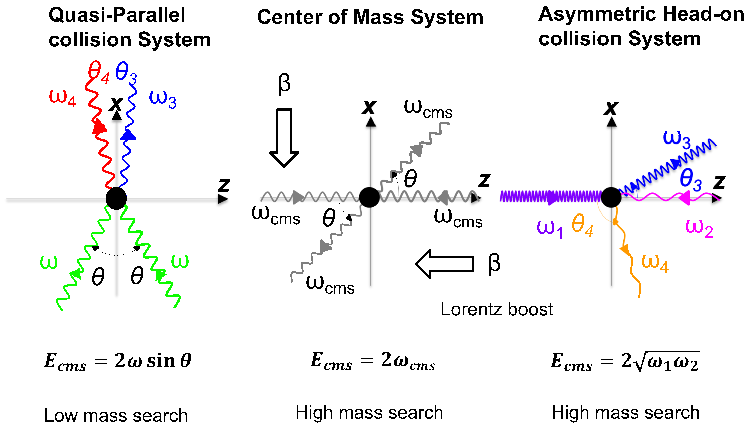
As the simplest example, let us first consider a head-on photon–photon collision at a center of mass system energy $2{\omega }_{cms}$ as illustrated in the middle of Figure 2. In this collision system, the initial and final state photons have the same photon energies. With respect to this collision system, if we introduce an observer who is moving along minus x-direction, the observer will see the collision geometry as indicated in the left of Figure 2. As a result of the Lorentz boost, the final state photons experience Doppler shifts: the one is blue shift and the other is red shift depending on the angles with respect to the boost direction. If we realize this Lorentz boosted frame in the laboratory, for instance, by introducing a lens element with respect to a single laser beam, the corresponding CMS energy is expressed as $E_{cms}=2\omega sin\vartheta$ with the laboratory photon energy $\omega$ and half incident angle between two photons $\vartheta$. Therefore, in addition to lowering photon energy, we can further lower the CMS energy by introducing a small incident angle, that is, with a long focal length. We refer to this collision system as Quasi Parallel collision System (QPS) in the following discussion. The feature of QPS is thus summarized as: it can lower the CMS energy by several orders of magnitude and it can cause photon energy shifts as a result of scattering, which can be a clear signature of scattering.

As a dilatonic scalar-type pNGB associated with conformal symmetry breaking, testability of the chameleon mechanism has been discussed in a recent paper [4] in order to explore the dark energy parameter spaces consistent with the cosmological observations. 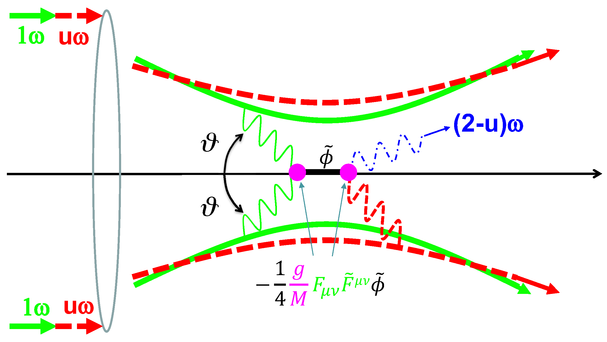In this paper, we focus on testability of the QCD axion [5,6,7,8,9], a pseudoscalar-type pNGB, associated with Peccei–Quinn symmetry breaking [5] as well as a generic axion-like particle relevant to a inflation scenario [10] as illustrated in Figure 3. The coupling of a pNGB with two photons is then expressed via the following interaction Lagrangian in the case of the pseudoscalar field ($\tilde{\varphi }$) exchange

$$-\mathcal{L}=\frac{1}{4}\frac{g}{M}{F}_{\mu \nu }{\tilde{F}}^{\mu \nu }\tilde{\varphi }.$$

(1)

Because we are interested in a very weak coupling domain relevant to dark components in the Universe, we have to accept a situation where even if a pNBG is produced, it cannot immediately decay into two photons spontaneously, that is, it can survive for a long time. We thus have proposed to introduce a co-moving coherent field in order to stimulate the pNGB decay [11]. Figure 3 indicates that a creation field with energy $\omega$ (solid green line) is combined with a different-color inducing field with energy $u\omega (0<u<1)$ (dashed red line). The combined fields are simultaneously focused by a lens element in a vacuum. Emission of signal photons with energy $(2-u)\omega$ (blue wavy line) is parametrically stimulated via energy–momentum conservation in the scattering process $\omega +\omega \to \tilde{\varphi }\to (2-u)\omega +u\omega$ via a resonance state $\tilde{\varphi }$. This stimulation effect will be discussed in detail in the next section.

Experimentally, if QPS is realized by focusing electromagnetic fields, we need to accept a situation where the incident momenta (angles) of photons largely fluctuate at around a focal point. This is due to the wavy nature of photons, that is, the uncertainty principle. In addition, as we discuss later, since we assume a short pulsed electromagnetic field reaching its Fourier transform limit, a pulsed beam must contain broad-band photons, that is, $\omega$ must also fluctuate. Therefore, it is unavoidable for the CMS energy in QPS to fluctuate in principle due to momentum (incident angle) fluctuations and also energy fluctuations simultaneously. This nature will be taken into account in the following calculation processes.

For simplicity, we have initially parametrized this stimulated resonant scattering in QPS by assuming symmetric incident angle and symmetric energy collisions [11] as shown in Figure 3. However, if we seriously consider the fluctuations on energy and momentum of incident two photons, we need to extend the symmetric scattering geometry to the fully asymmetric one where both a pair of photons with different momenta and energies creates a resonance state and its decay is stimulated by a field containing its momentum and energy fluctuation as well. This extension has been done in our previous publication ref. [12] in great detail.

In this paper, we will explore how much we can extend the present horizon in the weak coupling and low-mass domains by assuming multi-wavelengths coherent photon sources, which are in principle available at present and in the near future based on the parametrization in ref. [12]. As available photon sources for low energy photon–photon colliders, we will consider near-infrared laser fields at the eV scale, THz fields at the 0.01 eV scale, and GHz fields at the ${10}^{-5}$ eV scale in this paper. In the following section, we first review relevant formulae with some extensions to apply to the pseudoscalar-type field to describe the coupling-mass relation, and then provide the sensitivity projection in the end of the paper if we could utilize currently existing short-pulsed multi-wavelengths coherent beam sources with the near future extension.

2. Evaluation for the $\mathit{m}$–$\mathit{g}/\mathit{M}$ Relation in General QPS

In ref. [12], we have formulated stimulated resonant photon–photon scattering applicable to the most general collisional geometry including asymmetric incidence and non-coaxial scattering. The details are fully explained in the appendix of [12]. In the following subsections, we shortly summarize how to relate the physical parameters of mass m and coupling $g/M$ to the observed number of stimulated signal photons.

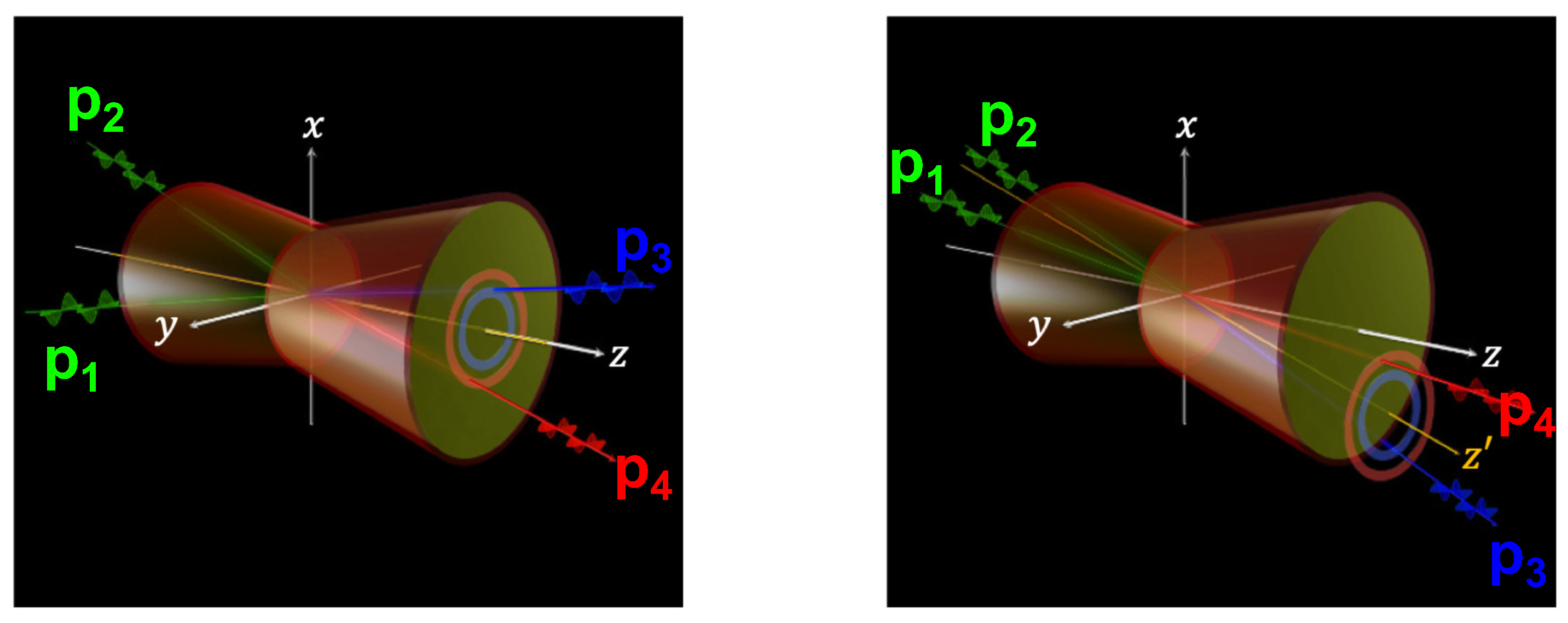
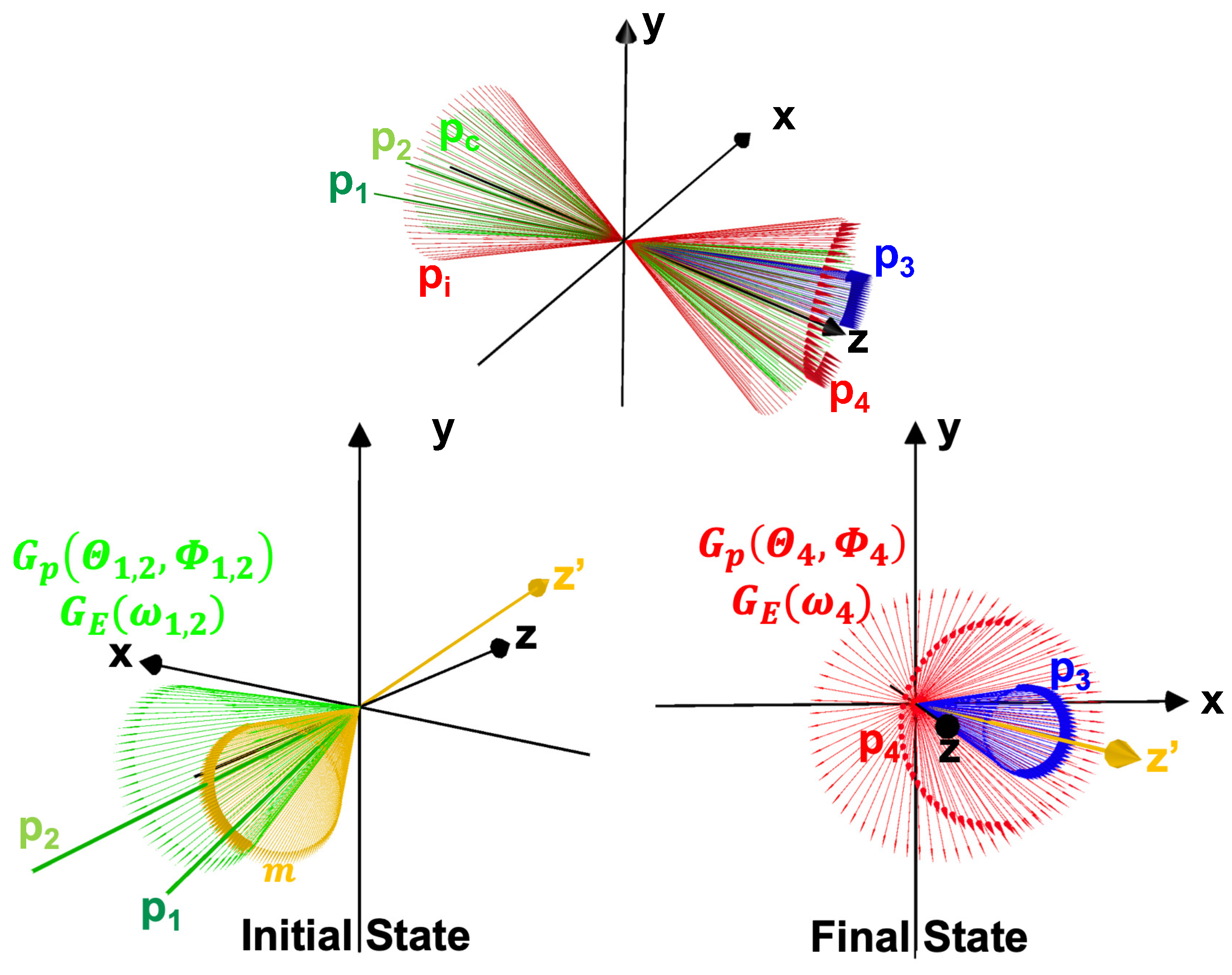
As illustrated in Figure 4, we consider a search for signal photons $p_3$ by mixing a creation beam with the central four-momentum $p_c$ and an inducing beam with the central four-momentum $p_i$ in a generic QPS:

$$<p_c\left(p_1\right)>+<p_c\left(p_2\right)>\to p_3+<p_i\left(p_4\right)>,$$

(2)

where $<>$ indicates that $p_1$ and $p_2$ are stochastically selected from the focused coherent beam for the creation of long-lived resonance states via s-channel photon–photon scattering, while the focused coherent beam is co-moving to induce emission of signal photons $p_3$ when a fraction of the $p_i$ beam coincides with $p_4$.

As depicted in Figure 4 (left), in symmetric incidence and coaxial scattering, transverse momenta of stochastically selected plane wave pairs, $p_T$, are always fixed to zero with respect to the common optical axis z. In this case, the evaluation of the inducible momentum or angular range can be very much simplified because the azimuthal angles of the final-state plane wave vectors are axially symmetric around the z-axis where the axial symmetry of the focused laser beams is also maintained. In the case of asymmetric incidence and non-coaxial scattering in Figure 4 (right), however, a finite transverse momentum must be introduced. Thus, the axial symmetry is lost. Even in this case, however, it is possible to find a new zero-$p_T$ axis, expressed as the $z^{{}^{\prime }}$-axis, for any pair of incident wave vectors. Around this $z^{{}^{\prime }}$-axis, thus, the axial symmetric nature of the azimuthal angles of the final-state wave vectors can be restored. On the other hand, since the inducing coherent field is still physically mapped on to the common optical axis z, depending on an arbitrarily formed $z^{{}^{\prime }}$-axis, the inducible momentum range changes. This situation complicates the evaluation of the induced signal yield. A numerical integration is thus necessary to estimate the number of signal photons generated from the creation of resonance state (c) and its induced decay (i) in the scattering process (2) per pulse collision, ${\mathcal{Y}}_{c+i}$. Given a ${\mathcal{Y}}_{c+i}$ with a set of coherent beam parameters P, the number of stimulated signal photons, $N_{obs}$, is expressed as

$$N_{obs}={\mathcal{Y}}_{c+i}(m,g/M;P)t_{a}rϵ,$$

(3)

as a function of mass m and coupling $g/M$, where $t_a$ is the data acquisition time, r is the repetition rate of the pulsed beams, and $ϵ$ is the overall efficiency of detecting $p_3$. For a set of m values and an $N_{obs}$, a set of coupling $g/M$ can be estimated by numerically solving the equation.

2.1. Induced Signal Yield ${\mathcal{Y}}_{c+i}$

The induced signal yield ${\mathcal{Y}}_{c+i}$ per pulse collision is expressed as

$$\begin{array}{c}\hfill {\mathcal{Y}}_{c+i}\left[1\right]=(N_c/2)(N_c/2)N_i\times \\ \hfill \left({\int }_{-Z_{R_c}/c}^{0}dt{\int }_{-\infty }^{+\infty }dr{\rho }_c(r,t){\rho }_c(r,t){\rho }_i(r,t)V_i\right)\times \\ \hfill \left(\int d{Q}_{I}W\left(Q_I\right)\frac{c}{2{\omega }_{1}2{\omega }_2}{|{\mathcal{M}}_s\left(Q^{{}^{\prime }}\right)|}^{2}d{L}_{ips}^{{}^{\prime }I}\right)\\ \hfill \equiv \frac{1}{4}{N}_c^2{N}_i{\mathcal{D}}_I\left[s/L^3\right]{\overline{\Sigma }}_I\left[L^3/s\right],\end{array}$$

(4)

where units are explicitly given in [ ] with units of length L and second s.

The factors $N_c$ and $N_i$ in Equation (4) are the average numbers of photons per pulse for the creation and inducing coherent beams, respectively. Theoretically the coherent states include Poissonian fluctuations of the numbers of photons around these mean numbers.

The factor ${\mathcal{D}}_I$ in Equation (4) expresses a spatiotemporal overlapping factor of the focused creation beam (subscript c) with the co-moving focused inducing beam (subscript i) in laboratory coordinates (see $x,y,z$ in Figure 5). The following photon number densities ${\rho }_{k=c,i}$ deduced from the electromagnetic field amplitudes based on the Gaussian beam parameterization are integrated over spacetime $(t,r)$:

$$\begin{array}{c}\hfill {\rho }_k(t,r)={\left(\frac{2}{\pi }\right)}^{\frac{3}{2}}\frac{1}{w_k^2\left(ct\right)c{\tau }_k}\times \\ \hfill exp\left(-2\frac{x^2+y^2}{w_k^2\left(ct\right)}\right)exp\left(-2{\left(\frac{z-ct}{c{\tau }_k}\right)}^2\right),\end{array}$$

(5)

where $w_k$ are the beam radii as a function of time t whose origin is set at the moment when all the pulses reach the focal point, and ${\tau }_k$ are the time durations of the pulsed laser beams with the speed of light c and the volume for the inducing beam $V_i$ is defined as

$$V_i={(\pi /2)}^{3/2}{w}_{i0}^{2}c{\tau }_i,$$

(6)

where $w_{i0}$ is the beam waist (minimum radius) of the inducing beam. As a conservative evaluation, the integrated range for the overlapping factor is limited in the Rayleigh length $z_{R_c}$ only around the focal spot of the creation field where the scattering probability is maximized. In concrete the factor ${\mathcal{D}}_{\mathit{I}}$ is given as follows:

$${\mathcal{D}}_{\mathit{I}}=\frac{1}{2}{\left(\frac{2}{\pi }\right)}^{\frac{3}{2}}\frac{1}{c^2}\frac{{\tau }_{\mathrm{i}}}{{\tau }_{\mathrm{c}}}\frac{1}{\sqrt{{\tau }_{\mathrm{c}}^2+2{\tau }_{\mathrm{i}}^2}}\frac{1}{w_{\mathrm{c}0}^2\left(1-\frac{z_{\mathrm{c}R}^2}{z_{\mathrm{i}R}^2}\right)}\left[z_{\mathrm{c}R}{tan}^{-1}\left(\frac{z_{\mathrm{i}R}}{z_{\mathrm{c}R}}\right)-R_{\mathrm{ci}}{Z}_{\mathrm{ci}}{tan}^{-1}\left(\frac{z_{\mathrm{i}R}}{Z_{\mathrm{ci}}}\right)\right]$$

(7)

with

$$R_{\mathrm{ci}}\equiv \frac{w_{\mathrm{c}0}^2{z}_{\mathrm{i}R}^2+2w_{\mathrm{i}0}^2{z}_{\mathrm{c}R}^2}{z_{\mathrm{i}R}^2\left(w_{\mathrm{c}0}^2+2w_{\mathrm{i}0}^2\right)}$$

(8)

and

$$Z_{\mathrm{ci}}\equiv \sqrt{\frac{w_{\mathrm{c}0}^2+2w_{\mathrm{i}0}^2}{{\vartheta }_{\mathrm{c}0}^2+2{\vartheta }_{\mathrm{i}0}^2}}$$

(9)

using beam diameters $d_{\mathrm{k}}$ for a common focal length f, beam waists $w_{\mathrm{k}0}$, wavelengths ${\lambda }_{\mathrm{k}}$ and Rayleigh lengths $z_{\mathrm{k}R}$ for $\mathrm{k}=\mathrm{c},\mathrm{i}$ defined as

$$\begin{array}{cc}\hfill {\vartheta }_{\mathrm{k}0}& ={tan}^{-1}\left(\frac{d_{\mathrm{k}}}{2f}\right),\hfill \end{array}$$

(10)

$$\begin{array}{cc}\hfill w_{\mathrm{k}0}& =\frac{{\lambda }_{\mathrm{k}}}{\pi {\vartheta }_{\mathrm{k}0}},\hfill \end{array}$$

(11)

$$\begin{array}{cc}\hfill z_{\mathrm{k}R}& =\frac{\pi w_{\mathrm{k}0}^2}{{\lambda }_{\mathrm{k}}}.\hfill \end{array}$$

(12)

We note that this ${\mathcal{D}}_I$ is the modified expression from that in ref. [12] for the different beam diameter case in order to fit to the real experimental setup [13] obtained by integrating the spatiotemporal overlapping factor in Equation (4) over the Rayleigh length of the inducing laser, which is longer than that of the creation laser in the experimental setup.

The factor ${\overline{\Sigma }}_I$ in Equation (4) describes an integrated inducible volume-wise interaction rate by integrating the square of the scattering amplitude $|{\mathcal{M}}_s\left(Q^{{}^{\prime }}\right){|}^2$ over an inducible variable set consisting of energies ${\omega }_i$, polar angles ${\Theta }_i$, and azimuthal angles ${\Phi }_i$ in laboratory coordinates for $i=1,2,4$: $Q_I\equiv \{Q,{\omega }_4,{\Theta }_4,{\Phi }_4\}$ with $Q\equiv \{{\omega }_1,{\Theta }_1,{\Phi }_1,{\omega }_2,{\Theta }_2,{\Phi }_2\}$ by weighting with multiple Gaussian distributions:

$$W\left(Q_I\right)\equiv {\mathsf{\Pi }}_i{G}_E\left({\omega }_i\right)G_p({\Theta }_i,{\Phi }_i)$$

(13)

for energy $G_E$ and for momentum $G_p$, and also over an inducible Lorentz-invariant phase space in zero-$p_T$ coordinates:

$$d{L}_{ips}^{{}^{\prime }I}={\left(2\pi \right)}^4\delta (p_3^{{}^{\prime }}+p_4^{{}^{\prime }}-p_1^{{}^{\prime }}-p_2^{{}^{\prime }})\frac{d^3{p}_3^{{}^{\prime }}}{2{\omega }_3{\left(2\pi \right)}^3}\frac{d^3{p}_4^{{}^{\prime }}}{2{\omega }_4{\left(2\pi \right)}^3}$$

(14)

with two incident energies ${\omega }_1$ and ${\omega }_2$. The primed variables $Q^{{}^{\prime }}$ in zero-$p_T$ coordinates can be converted from Q in laboratory coordinates via coordinate rotation. The energy and momentum fractions of $p_4$ satisfying energy–momentum conservation with respect to the energy and momentum distributions of the given inducing laser beam in laboratory coordinates are taken into account in the inducing weight $W\left(Q_I\right)$. The fundamental element of ${\overline{\Sigma }}_I$ is the Lorentz-invariant scattering amplitude defined in zero-$p_T$ coordinates, ${\mathcal{M}}_S\left(Q^{{}^{\prime }}\right)$, for the given polarization states $S=abcd$ in a two-body interaction: $p_1^{{}^{\prime }}\left\{a\right\}+p_2^{{}^{\prime }}\left\{b\right\}\to p_3^{{}^{\prime }}\left\{c\right\}+p_4^{{}^{\prime }}\left\{d\right\}$. In the following, unless confusion is expected, the prime symbol associated with the momentum vectors will be omitted.

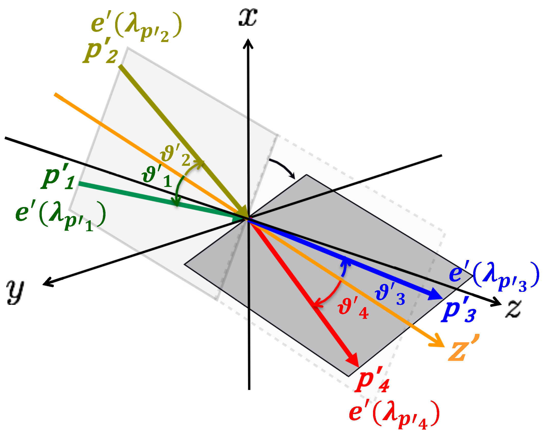
2.2. Derivation of $|{\mathcal{M}}_s\left(Q^{{}^{\prime }}\right){|}^2$

We review the relevant formulae for the scalar-field exchange in ref. [12] to describe the scattering amplitude based on the kinematic definitions in Figure 5 and then extend them to the pseudo-scalar field exchange in the following. The second order term in the expansion of the scattering operator for the scalar type effective interaction Lagrangian

$$-\mathcal{L}=g{M}^{-1}\frac{1}{4}{F}_{\mu \nu }{F}^{\mu \nu }\varphi$$

(15)

is expressed as

$$\begin{array}{c}\hfill S^{\left(2\right)}={\left(-\frac{1}{4}\frac{g}{M}\right)}^2\frac{i^2}{2}\int d^{4}x\int d^{4}y\\ \hfill \times T\left[F_{\mu \nu }\left(x\right)F^{\mu \nu }\varphi \left(x\right)F_{\rho \sigma }\left(y\right)F^{\rho \sigma }\left(y\right)\varphi \left(y\right)\right],\end{array}$$

(16)

where T is the time-ordered product. The T-product can be converted to the normal-ordering product by requiring contractions with four external electromagnetic fields based on Wick’s theorem as follows:

$$N[F_{\mu \nu }\left(x\right)F^{\mu \nu }\left(x\right)F_{\sigma \rho }\left(y\right)F^{\sigma \rho }\left(y\right)\langle 0\left|T\left[\varphi \left(x\right)\varphi \left(y\right)\right]\right|0\rangle ],$$

(17)

where

$$i\langle 0\left|T\left[\varphi \left(x\right)\varphi \left(y\right)\right]\right|0\rangle \equiv \frac{1}{{\left(2\pi \right)}^4}\int d^{4}q\frac{e^{-iq(x-y)}}{m_{\varphi }^2-q^2-iϵ}$$

(18)

is the propagator of a massive scalar field $\varphi$ with the mass $m_{\varphi }$ and infinitesimal number $ϵ$. The field strength tensor is then expanded as

$$F^{\mu \nu }\equiv (-i)\int \frac{d^3\mathit{p}}{{\left(2\pi \right)}^{3}2p^0}{\Sigma }_{\lambda =1,2}(P^{\mu \nu }{e}^{-ipx}{a}_{\mathit{p},{\lambda }_p}+{\widehat{P}}^{\mu \nu }{e}^{ipx}{a}_{\mathit{p},{\lambda }_p}^{†})$$

(19)

with a polarization four-vector $e_i\left({\lambda }_p\right)$ with an arbitrary polarization state ${\lambda }_p$ associated with a four-momentum p and a symbol * indicating complex conjugate, the momentum-polarization tensors are defined as

$$\begin{array}{ccc}\hfill P^{\mu \nu }\left({\lambda }_p\right)& \equiv & p^{\mu }{e}^{\nu }\left({\lambda }_p\right)-e^{\mu }\left({\lambda }_p\right)p^{\nu },\hfill \\ \hfill {\widehat{P}}^{\mu \nu }\left({\lambda }_p\right)& \equiv & e^{\ast \mu }\left({\lambda }_p\right)p^{\nu }-p^{\mu }{e}^{\ast \nu }\left({\lambda }_p\right).\hfill \end{array}$$

(20)

We also can apply the same formation based on the following pseudo scalar type effective Lagrangian

$$-\mathcal{L}=g{M}^{-1}\frac{1}{4}{F}_{\mu \nu }{\tilde{F}}^{\mu \nu }\tilde{\varphi }$$

(21)

resulting in

$$\begin{array}{c}\hfill {\tilde{S}}^{\left(2\right)}={\left(-\frac{1}{4}\frac{g}{M}\right)}^2\frac{i^2}{2}\int d^{4}x\int d^{4}y\\ \hfill \times T[F_{\mu \nu }\left(x\right){\tilde{F}}^{\mu \nu }\tilde{\varphi }\left(x\right)F_{\rho \sigma }\left(y\right){\tilde{F}}^{\rho \sigma }\left(y\right)\tilde{\varphi }\left(y\right)]\end{array}$$

(22)

with the pseudo scalar type propagator

$$i\langle 0|T[\tilde{\varphi }\left(x\right)\tilde{\varphi }\left(y\right)]|0\rangle \equiv \frac{1}{{\left(2\pi \right)}^4}\int d^{4}q\frac{e^{-iq(x-y)}}{m_{\tilde{\varphi }}^2-q^2-iϵ}$$

(23)

where the dual field strength tensor is defined as

$${\tilde{F}}^{\mu \nu }\equiv {ϵ}^{\mu \nu \alpha \beta }{F}_{\alpha \beta }=(-i)\int \frac{d^{3}p}{{\left(2\pi \right)}^{3}2p^0}{\Sigma }_{\lambda =1,2}({\tilde{P}}^{\mu \nu }{e}^{-ipx}{a}_{p,{\lambda }_p}+{\widehat{\tilde{P}}}^{\mu \nu }{e}^{ipx}{a}_{p,{\lambda }_p}^{†})$$

(24)

with the corresponding momentum-polarization tensors

$$\begin{array}{ccc}\hfill {\tilde{P}}^{\mu \nu }\left({\lambda }_p\right)& \equiv & {\epsilon }^{\mu \nu \alpha \beta }\left(p_{\alpha }{e}_{\beta }\left({\lambda }_p\right)-e_{\alpha }\left({\lambda }_p\right)p_{\beta }\right),\hfill \\ \hfill {\widehat{\tilde{P}}}^{\mu \nu }\left({\lambda }_p\right)& \equiv & {\epsilon }^{\mu \nu \alpha \beta }\left(p_{\alpha }{e}_{\beta }^{\ast }\left({\lambda }_p\right)-e_{\alpha }^{\ast }\left({\lambda }_p\right)p_{\beta }\right).\hfill \end{array}$$

(25)

The following commutation relations are required to creation and annihilation operators for both the effective interactions which become important for the discussion of the simulation effect.

$$\begin{array}{ccc}\hfill [a_{\mathit{p},{\lambda }_p},a_{{\mathit{p}}^{{}^{\prime }},{\lambda }_p^{{}^{\prime }}}^{†}]& =& {\left(2\pi \right)}^{3}2p^0{\delta }^3(\mathit{p}-{\mathit{p}}^{{}^{\prime }})\delta ({\lambda }_p-{\lambda }_p^{{}^{\prime }}),\hfill \\ \hfill [a_{\mathit{p},{\lambda }_p},a_{{\mathit{p}}^{{}^{\prime }},{\lambda }_p^{{}^{\prime }}}]& =& [a_{\mathit{p},{\lambda }_p}^{†},a_{{\mathit{p}}^{{}^{\prime }},{\lambda }_p^{{}^{\prime }}}^{†}]=0.\hfill \end{array}$$

(26)

From here, we omit the polarization index $\lambda$ and the sum over it for the photon creation and annihilation operators, $a_{\mathit{p},\lambda }$ and $a_{\mathit{p},\lambda }^{†}$, because we require fixed beam polarizations in the last step of the following calculations.

The coherent state [14] is defined as

$$|N_{\mathit{p}}\rangle \rangle \equiv exp\left(-N_{\mathit{p}}/2\right)\sum _{n=0}^{\infty }\frac{N_{\mathit{p}}^{n/2}}{\sqrt{n!}}|n_{\mathit{p}}\rangle ,$$

(27)

where $|n_{\mathit{p}}\rangle$ is the normalized state of n photons

$$|n_{\mathit{p}}\rangle =\frac{1}{\sqrt{n!}}{\left(a_{\mathit{p}}^{†}\right)}^n|0\rangle ,$$

(28)

with the creation operator $a_{\mathit{p}}^{†}$ of photons that share a common momentum p and a common polarization state over different number states. The following relations on the coherent state

$$\langle \langle N_{\mathit{p}}|N_{\mathit{p}}\rangle \rangle =1$$

(29)

and

$$\langle \langle N_{\mathit{p}}\left|n\right|N_{\mathit{p}}\rangle \rangle =\langle \langle N_{\mathit{p}}|\left(a_{\mathit{p}}^{†}{a}_{\mathit{p}}\right)|N_{\mathit{p}}\rangle \rangle =N_{\mathit{p}},$$

(30)

give us basic properties with respect to the creation and annihilation operators:

$$a_{\mathit{p}}|N_{\mathit{p}}\rangle \rangle =\sqrt{N_{\mathit{p}}}|N_{\mathit{p}}\rangle \rangle ,\mathrm{and}\langle \langle N_{\mathit{p}}|a_{\mathit{p}}^{†}=\sqrt{N_{\mathit{p}}}\langle \langle N_{\mathit{p}}|.$$

(31)

A search for signal photons $p_3$ is considered via the scattering process $p_1+p_2\to p_3+p_4$ by supplying coherent fields $|N_{{\mathit{p}}_1}\rangle \rangle$, $|N_{{\mathit{p}}_2}\rangle \rangle$ and $|N_{{\mathit{p}}_4}\rangle \rangle$. The initial and final states are, respectively, introduced as follows:

$$\begin{array}{ccc}\hfill |\Omega \rangle & \equiv & |N_{{\mathit{p}}_1}\rangle \rangle |N_{{\mathit{p}}_2}\rangle \rangle |N_{{\mathit{p}}_4}\rangle \rangle |0\rangle ,\mathrm{and}\hfill \\ \hfill \langle {\Omega }^{{}^{\prime }}|& \equiv & \langle \langle N_{{\mathit{p}}_1}|\langle \langle N_{{\mathit{p}}_2}|\langle \langle N_{{\mathit{p}}_4}|\langle 1_{{\mathit{p}}_3}|=\langle \Omega |a_{{\mathit{p}}_3}.\hfill \end{array}$$

(32)

In the following, we commonly formulate a Lorentz-invariant scattering amplitude both for exchanges of scalar and pseudoscalar fields with a mass m by omitting the field-type subscript with a sequence of four-photon polarization states as a subscript $S\equiv abcd$ for the initial $a,b$ and the final $c,d$ states. From the following definition for the transition amplitude

$$\begin{array}{c}\hfill \langle {\Omega }^{{}^{\prime }}|S_{2\to 2}^{\left(2\right)}|\Omega \rangle =\sqrt{N_{p_1}}\sqrt{N_{p_2}}\sqrt{N_{p_4}}\times \\ \hfill i{\left(2\pi \right)}^4{\delta }^{\left(4\right)}(p_1+p_2-p_3-p_4){\mathcal{M}}_S,\end{array}$$

(33)

with the initial and final state vertex factors $V_i$ and $V_f$, respectively, the s-channel Lorentz-invariant scattering amplitude ${\mathcal{M}}_S$ can be expressed as

$$\begin{array}{cc}\hfill {\mathcal{M}}_S& =\frac{1}{4}{\left(\frac{g}{M}\right)}^2\frac{V_i{V}_f}{m^2-2{\omega }_1{\omega }_2(1-cos({\vartheta }_1+{\vartheta }_2))}\hfill \\ \hfill & =\frac{1}{4}{\left(\frac{g}{M}\right)}^2\frac{V_i{V}_f}{m^2-4{\omega }_1{\omega }_2{sin}^2{\vartheta }_b}\hfill \end{array}$$

(34)

with ${\vartheta }_b\equiv ({\vartheta }_1+{\vartheta }_2)/2$. To implement energy fluctuations in the initial state of two photons chosen from a solo coherent beam around its central energy ${\omega }_c$, we introduce two independent parameters $s_1$ and $s_2$, as follows:

$${\omega }_1=s_1{\omega }_{\mathrm{c}},{\omega }_2=s_2{\omega }_{\mathrm{c}}.$$

(35)

We then define a resonance energy ${\omega }_r$ satisfying $E_{cms}=m$ as

$${\omega }_r^2\equiv \frac{m^2}{4s_1{s}_2{sin}^2{\vartheta }_b}.$$

(36)

Because the exchanged scalar field is (in principle) an unstable particle, we introduce a decay rate $\Gamma$, which is defined as [11]

$$\Gamma =\frac{1}{16\pi }{\left(\frac{g}{M}\right)}^2{m}^3.$$

(37)

This causes a change in the mass square as $m^2\to {(m-i\Gamma /2)}^2\approx m^2-im\Gamma$. Therefore, the denominator $\mathcal{D}$ in Equation (34) is expressed as

$$\begin{array}{cc}\hfill \mathcal{D}& \approx -4s_1{s}_2{\omega }_{\mathrm{c}}^2{sin}^2{\vartheta }_b+m^2-i\Gamma m\hfill \\ \hfill & =-4s_1{s}_2{\omega }_{\mathrm{c}}^2{sin}^2{\vartheta }_b+4s_1{s}_2{\omega }_r^2{sin}^2{\vartheta }_b-i\Gamma m\hfill \\ \hfill & =-4s_1{s}_2{sin}^2{\vartheta }_b\left({\omega }_{\mathrm{c}}^2-{\omega }_r^2+i\frac{\Gamma m}{4s_1{s}_2{sin}^2{\vartheta }_b}\right)\hfill \\ \hfill & \equiv -4s_1{s}_2{sin}^2{\vartheta }_b(\chi +ia),\hfill \end{array}$$

(38)

where

$$\chi \equiv {\omega }_c^2-{\omega }_r^2=\left(1-\frac{m^2}{4{\omega }_1{\omega }_2{sin}_{{\vartheta }_b}^2}\right){\omega }_c^2$$

(39)

describes the degrees of deviation of $E_{cms}$ as determined by a pair of incident photons from the resonance energy derived from the central energy ${\omega }_c$, and a is defined as

$$a=\frac{\Gamma m{\omega }_c^2}{4{\omega }_1{\omega }_2{sin}^2{\vartheta }_b}=\frac{1}{16\pi }{\left(\frac{g}{M}\right)}^2{\omega }_r^2{m}^2.$$

(40)

By using a, the invariant amplitude is re-expressed as

$${\mathcal{M}}_S=-4\pi \frac{a}{\chi +ia}\left(\frac{V_i}{m^2}\right)\left(\frac{V_f}{m^2}\right)\equiv \mathcal{M}{\mathcal{V}}_i{\mathcal{V}}_f$$

(41)

where the polarization-independent amplitude $\mathcal{M}$ and the vertex coefficients ${\mathcal{V}}_i$ and ${\mathcal{V}}_f$ are introduced. We then take square of ${\mathcal{M}}_S$ expressed as

$$|{\mathcal{M}}_s{|}^2={\left|\mathcal{M}\right|}^2{\mathcal{V}}_i^2{\mathcal{V}}_f^2$$

(42)

where ${\left|\mathcal{M}\right|}^2$ contains the Breit–Wigner formula as a function of $\chi$ with the resonance width of a

$${\left|\mathcal{M}\right|}^2={\left(4\pi \right)}^2\frac{a^2}{{\chi }^2+a^2}.$$

(43)

Because $E_{cms}$ is in principle uncertain due to unavoidable energy and momentum uncertainties of a selected pair of photon wave vectors in QPS, averaging the resonance effect over a range of $\chi$ is necessary. In order to demonstrate the essence of inclusion of a resonance state within a range from ${\chi }_{-}$ to ${\chi }_{+}$, we show the simplest averaging process as follows. Defining ${\chi }_{\pm }$ in units of a as ${\chi }_{\pm }=\pm \eta a$ with $\eta \gg 1$ the averaging is then expressed as

$$\begin{array}{ccc}\hfill \overline{{\left|\mathcal{M}\right|}^2}& =& \frac{1}{{\chi }_{+}-{\chi }_{-}}{\int }_{{\chi }_{-}}^{{\chi }_{+}}{\left|M\right|}^{2}d\chi \hfill \\ \hfill & =& \frac{{\left(4\pi \right)}^2}{2\eta a}2a{tan}^{-1}\left(\eta \right)={\left(4\pi \right)}^2{\eta }^{-1}{tan}^{-1}\left(\eta \right)\hfill \\ \hfill & \approx & {\left(4\pi \right)}^2{\eta }^{-1}\frac{\pi }{2}=8{\pi }^2\frac{a}{|{\chi }_{\pm }|},\hfill \end{array}$$

(44)

where the approximation is due to $\eta \gg 1$. Capturing a resonance within the $E_{cms}$ uncertainty has an obvious gain of $a^{-1}\propto M^2$ compared to non s-channel cases where ${\left|\mathcal{M}\right|}^2\propto a^2$. Since we are interested in the energy scale M corresponding to the Planckian scale $M_p$, this gain factor is huge even though we cannot directly hit the top of the Breit–Wigner distribution where ${\left|\mathcal{M}\right|}^2\propto {\left(4\pi \right)}^2$ with $\chi \to 0$. This is the significant impact of s-channel scattering including a resonance in QPS. Indeed, we have already introduced $W\left(Q_I\right)$ in Equation (13) to Equation (4) as more realistic probability distribution functions based on the physical nature of propagating electromagnetic fields in order to effectively implement this averaging process.

2.3. Vertex Factors

Based on Figure 5 arbitrary momentum-polarization tensor products between four-momenta s and t with their polarization states ${\lambda }_s$ and ${\lambda }_t$ are summarized as

$$\begin{array}{ccc}\hfill S_{\mu \nu }\left({\lambda }_s\right)T^{\mu \nu }\left({\lambda }_t\right)& =& 2\{(s·t)(e\left({\lambda }_s\right)·e\left({\lambda }_t\right))-(s·e\left({\lambda }_t\right))(t·e\left({\lambda }_s\right))\},\hfill \\ \hfill {\widehat{S}}_{\mu \nu }\left({\lambda }_s\right){\widehat{T}}^{\mu \nu }\left({\lambda }_t\right)& =& 2\{(s·t)(e^{\ast }\left({\lambda }_s\right)·e^{\ast }\left({\lambda }_t\right))-(s·e^{\ast }\left({\lambda }_t\right))(t·e^{\ast }\left({\lambda }_s\right))\}\hfill \end{array}$$

(45)

for scalar field exchange and

$$\begin{array}{ccc}\hfill S_{\mu \nu }\left({\lambda }_s\right){\tilde{T}}^{\mu \nu }\left({\lambda }_t\right)& =& 4{\epsilon }^{\mu \nu \alpha \beta }{s}_{\mu }{e}_{\nu }\left({\lambda }_s\right)t_{\alpha }{e}_{\beta }\left({\lambda }_t\right),\hfill \\ \hfill {\widehat{S}}_{\mu \nu }\left({\lambda }_s\right){\widehat{\tilde{T}}}^{\mu \nu }\left({\lambda }_t\right)& =& 4{\epsilon }^{\mu \nu \alpha \beta }{s}_{\mu }{e}_{\nu }^{\ast }\left({\lambda }_s\right)t_{\alpha }{e}_{\beta }^{\ast }\left({\lambda }_t\right)\hfill \end{array}$$

(46)

for pseudoscalar exchange. With the abbreviated expression $\left(ST\right)$ representing a momentum-polarization tensor product such as $\left(ST\right)\equiv S_{\mu \nu }{T}^{\mu \nu }$ for four-momenta s and t, the concrete vertex factors in Equation (34) are given as

$$V_i{V}_f=\left(P_1{P}_2\right)\left({\widehat{P}}_3{\widehat{P}}_4\right)$$

(47)

for the scalar field exchange and

$$V_i{V}_f=\left(P_1{\tilde{P}}_2\right)\left({\widehat{P}}_3{\widehat{\tilde{P}}}_4\right)$$

(48)

for the pseudoscalar field exchange. In the following calculation scheme, these vertex factors are numerically calculated for a given set of four-momentum vectors and polarization vectors in the process of the calculation.

2.4. Flow of Numerical Calculations

Based on Figure 6 (top) where wave vector directions contained in the focused creation (green) and inducing (red) fields and signal wave vectors (blue) are drawn in the laboratory coordinates, the steps in the numerical calculation including fully asymmetric collisions are explained below. With G representing normalized Gaussian distributions, probability distribution functions in momentum space $G_p$ as a function of polar angles ${\Theta }_i$ and azimuthal angles ${\Phi }_i$ mapped on the laboratory coordinates and those in energy $G_E\left({\omega }_i\right)$ for the creation (left, green) and inducing (right, red) lasers for individual photons $i=1,2,4$ are implemented for individual focused fields. The concrete steps are summarized as follows:

• Choose a finite-size segment of $p_1$ based on the $G_E\left({\omega }_1\right)G_p({\Theta }_1,{\Phi }_1)$ distributions.
• A $z^{{}^{\prime }}$-axis of zero-$p_T$ coordinates denoted as the yellow arrow in the left figure is defined by paring $p_2$ that satisfies the resonance condition with respect to the selected $p_1$ and to a finite energy segment from $G_E\left({\omega }_2\right)$ for a given mass parameter m. The yellow cone around the $p_1$-axis in the left figure indicates possible $p_2$ candidates satisfying the resonance condition. Effectively, creation fields along the thicker yellow arc belt crossing with the creation angular distribution can contribute to the resonance creation and thus the proper field weights for $p_1$ and $p_2$ are taken into account.
• Convert the polarization vectors $e_i\left({\lambda }_i\right)$ from laboratory coordinates to zero-$p_T$ coordinates through coordinate rotation $Q\to Q^{{}^{\prime }}$.
• The axial symmetric nature of possible final-state momenta $p_3^{{}^{\prime }}$ and $p_4^{{}^{\prime }}$ around $z^{{}^{\prime }}$ is drawn in the right figure. A spontaneous scattering probability with the vertex factors $V_i$ and $V_f$ in the planes containing four photo-waves (see Figure 5) is calculated in the given zero-$p_T$ coordinates and it is integrated over possible final state planes containing $p_3^{{}^{\prime }}$ and $p_4^{{}^{\prime }}$ by utilizing the axial symmetric nature around $z^{{}^{\prime }}$.
• To evaluate the inducing effect with respect to $G_E\left({\omega }_4\right)G_p({\Theta }_4,{\Phi }_4)$ defined in the laboratory coordinates, a matching fraction of $p_4$ is calculated after rotating back to the laboratory coordinates from the zero-$p_T$ coordinates by $Q^{{}^{\prime }}\to Q$. Based on the spread of $G_E\left({\omega }_4\right)$, weights along the red arc belt (Figure 6 right) are determined via energy–momentum conservation.
• Because $p_3$ must balance with $p_4$ through energy–momentum conservation, a signal energy spread via ${\omega }_s\equiv {\omega }_3={\omega }_1+{\omega }_2-{\omega }_4$ and also the polar-azimuthal angle spreads by taking the $G_E\left({\omega }_4\right)G_p({\Theta }_4,{\Phi }_4)$ distribution into account are parametrically determined. The volume-wise interaction rate ${\overline{\Sigma }}_I$ is then integrated over the inducible solid angle of $p_3$ calculated from all the energy and angular spreads.
• Based on Equation (4), the signal yield ${\mathcal{Y}}_{c+i}$ is evaluated.

3. Technology Choices for Photon Sources and Sensors

As explicitly shown in Equation (4), the signal yield is proportional to the square of the number of creation photons and the number of inducing photons per pulse. This cubic dependence on the pulse energies discriminates the proposed method from any existing charged particle colliders where the signal yield is proportional to square of the number of charged particles per colliding bunch in accelerators. Even in the case of fixed target experiments, this square dependence is still the same. Typically, the number of charged particles in a colliding bunch is at most order of ${10}^{11}$ due to the physical limitation by the space-charge effect in the focused beam. In the case of photons, however, there is no physical limitation at a focal point unless it reaches the Schwinger limit around ${10}^{29}$ W/cm${}^2$, above which pair productions may occur. Even with the highest laser intensities currently available at the Extreme Light Infrastructure (ELI) project [15], the reachable intensity is at most ${10}^{24}$ W/cm${}^2$ with a typical pulse energy of $0.1$–1 kJ and the pair production is still far from the threshold. However, this pulse energy already contains around ${10}^{21}$ near-infrared laser photons (∼800 nm) per pulse. The cubic of this number, ${\left({10}^{21}\right)}^3$, is huge compared to ${\left({10}^{11}\right)}^2$. We thus see the potential of this method to extend the present horizon of particle physics toward the very weakly coupling domains. Therefore, the beam energy per pulse is the essentially important factor for the stimulated photon–photon scattering probability to drastically increase.

A short pulse duration time at a focused geometry is another important factor through the inducible volume-wise interaction rate ${\overline{\Sigma }}_I$ and the overlapping factor ${\mathcal{D}}_I$ in Equation (4). The Fourier transform limited pulse duration is equivalent to the state with the maximally broadened energy spectrum and a focused beam introduces the uncertainty of incident angles, that is, momentum fluctuations. Thanks to these energy and momentum fluctuations, ${\overline{\Sigma }}_I$ drastically increases because the inducible kinematical phase space which can satisfy energy–momentum conservation between four-photons is enlarged. In addition, as seen in Equation (7), the overlapping factor is inversely proportional to the duration times of focused beams. Therefore, utilizing the Fourier transform limited pulse is the essential factor as well.

Taking the aforementioned two important factors into account, we seek for available coherent photon sources and discuss the individual single photon sensitivities as follows. For the near-infrared band (eV-band), as already introduced, pulsed laser fields are available at ELI facilities for instance. For this frequency domain, photomultipliers are widely used and well-known to be sensitive to single photons. For the THz band (0.01 eV-band), we consider to utilize THz beams produced via optical rectification driven by short-pulsed laser pumping. There is a possibility to generate tens-of-mJ level THz pulses as evaluated in [16]. The single photon sensitivity in the THz band is known to be achievable, for instance, based on nanostructured semiconductors and carbon materials [17]. As for the GHz band (${10}^{-5}$ eV-band), for instance, 100 MW-class klystron [18] is already available as commercial products though the pulse duration is still $\mathsf{\mu }$s level, which does not reach the Fourier transform limit corresponding to ns level. However, it is expected to be possible in principle if a pulse compression technique with a helically corrugated waveguide [19] is combined with a broad band klystron. Concerning the single photon sensitive device, for example, proof-of-principle detection is achieved based on an artificial $\Lambda$ system formed by the dressed states of a driven superconducting qubit coupled to a microwave resonator [20].

Given the discussion above, we assume coherent photon sources with individual single photon sensitivities as summarized in

Table 1. Photon beam parameters and experimental conditions used to create Figure 7.

Characteristic		Near-Infrared		THz-Band		GHz-Band (Compressed)
of Light Sources		Creation	Inducing	Creation	Inducing	Creation	Inducing
Central wavelength	${\lambda }_{c,i}$	$800\mathrm{nm}$	$1300\mathrm{nm}$	$259\mathsf{\mu }\mathrm{m}$	$422\mathsf{\mu }\mathrm{m}$	$4.15\mathrm{cm}$	$6.75\mathrm{cm}$
Relative line width	$\delta \nu /\nu$	$2.0\%$	$2.0\%$	$2.0\%$	$2.0\%$	$2.2\times {10}^{-3}\%$	$3.6\times {10}^{-3}\%$
						$(2.0\%)$	$(2.0\%)$
Energy per pulse	$E_{c,i}$	$10\mathrm{J}$	$10\mathrm{J}$	$10\mathrm{mJ}$	$10\mathrm{mJ}$	$100\mathrm{J}$	$100\mathrm{J}$
Pulse duration	${\tau }_{c,i}$	$21\mathrm{fs}$	$35\mathrm{fs}$	$6.9\mathrm{ps}$	$11.2\mathrm{ps}$	$1\mathsf{\mu }\mathrm{s}$	$1\mathsf{\mu }\mathrm{s}$
						$\left(1.1\mathrm{ns}\right)$	$\left(1.8\mathrm{ns}\right)$
Beam diameter	$d_{c,i}$	$25\mathrm{cm}$	$25\mathrm{cm}$	$5\mathrm{cm}$	$5\mathrm{cm}$	$3.0\mathrm{m}$	$3.0\mathrm{m}$
Experimental condition
Focal length	f	$125\mathrm{cm}$		$25\mathrm{cm}$		$15\mathrm{m}$
Repetition rate	r	$1\mathrm{Hz}$		$1\mathrm{Hz}$		$50\mathrm{Hz}$
Data acquisition time	$t_a$	$1\mathrm{month}$		$1\mathrm{month}$		$1\mathrm{month}$
Detector efficiency	$ϵ$	$5\%$		$5\%$		$5\%$
Required background level	$\delta N_S$	100		100		100

.

4. Sensitivity Projections

Based on parameters in Table 1, Figure 7 shows the reachable sensitivities in the coupling-mass relation for the pseudoscalar field exchange at a 95% confidence level by the concept of the stimulated resonant photon colliders with multi-wavelengths coherent photon sources represented as SRPCs in the figure. The red solid curve shows the excluded region by a SRPC, the SAPPHIRES collaboration [13]. The red dotted lines from the left are evaluated based on the GHz band (klystron), the THz band (optical rectification with short laser pulses), and the near-infrared band (lasers), respectively, whose parameters are all summarized in Table 1. These assumed photon sources all exist within the current technology in terms of the photons’ wavelengths and fields’ energies per pulse. In particular the thicker red dotted line indicates the case when an existing pulse from a high-power klystron [18] is compressed in time down to its Fourier transform limit. All the red dotted lines assume that single photon sensitivities of photon detectors in individual bands are guaranteed. We emphasize that the GHz sensitivity with the pulse compress can explore the gravitationally weak domain.

These sensitivity curves are obtained based on the following evaluation. In order to exclude a null hypothesis, a confidence level $1-\alpha$ is introduced as

$$1-\alpha =\frac{1}{\sqrt{2\pi }\sigma }{\int }_{\mu -\delta }^{\mu +\delta }{e}^{-{(x-\mu )}^2/\left(2{\sigma }^2\right)}dx=\mathrm{erf}\left(\frac{\delta }{\sqrt{2}\sigma }\right),$$

(49)

where $\mu$ is the expected value of an estimator x following a hypothesis, and $\sigma$ is one standard deviation. In searches, the estimator x corresponds to the number of signal photons $N_S$ and we assign the acceptance-uncorrected uncertainty $\delta N_S$ as the one standard deviation $\sigma$ around the mean value $\mu =0$. In these virtual searches, the null hypothesis is supposed to be fluctuations of the number of photon-like signals following a Gaussian distribution whose expectation value, $\mu$, is zero for the given total number of collision statistics. In order to settle a confidence level of 95%, $2\alpha =0.05$ with $\delta =2.24\sigma$ is used, where a one-sided upper limit by excluding above $x+\delta$ [41] is applied. The upper limits on the coupling–mass relation are then obtained by solving

$$N_{obs}=2.24\delta N_S={\mathcal{Y}}_{c+i}(m,g/M;P)t_{a}rϵ$$

(50)

numerically based on Equation (3) with respect to m and $g/M$ for a set of experimental parameters P in Table 1.

The rest of excluded domains and the future projections are explained as follows. All the solid lines are excluded regions by the past searching experiments, while all the dashed lines are ongoing searches and all the dotted lines indicate future experiments to which designs or concepts are proposed. The blue domains are excluded by the light shining through the wall (LSW) experiments represented by ALPS-I, II [21,22] and OSQAR [23]. The domain with the black solid line is excluded by the vacuum magnetic birefringence measurement represented by PVLAS-FE [24]. The domain with the green solid line is excluded by the Helioscope experiment CAST [25] with the future extentions by BabyIAXO and IAXO [26]. The magenta domains ares excluded by the Haloscopes experiments ADMX [27,28,29,30], RBF [31,32], UF [33], HAYSTAC [34,35], and the magenta dotted line indicates the projection by ADMX-G2 [36]. The purple domain is excluded by ABRACADABRA [37] and its extensions are the purple dashed lines ABRA-40 cm, ABRA-1 m, and ABRA-QCD [38]. The yellow band shows QCD axion models with $0.07<|E/N-1.95|<7$ where KSVZ($E/N=0$) [8,9] and DFSZ($E/N=8/3$) [39,40] are shown with the brawn lines. The cyan lines show predictions from an inflaton model, MIRACLE [10] with its parameters $c=1.0,0.1,0.01$, respectively. The gray area below ∼$3\times {10}^{-21}{\mathrm{GeV}}^{-1}$ represents the gravitationally weak coupling domain.

5. Conclusions

In this paper, we have introduced the concept of the stimulated photon–photon colliders and briefly reviewed how to evaluate the coupling-mass relation with respect to the observed number of signal photons by extending the formulae for the scalar field exchange to the pseudoscalar case. We then presented the sensitivity projections with multi-wavelength coherent photon sources in near-infrared, THz, and GHz frequency domains. Because the larger number of photons for a given common pulse energy is expected in the lower frequency band, the photon source in the GHz band shows a capability of accessing to the gravitationally weak coupling domain if the pulse compression technique in addition to the single-photon detection capability in GHz is realized, which allows a test of dark energy models [4]. As shown in Figure 7, within presently available beam intensities, we found that the QCD axion scenarios are thoroughly testable in the wide mass range: ${10}^{-6}$–${10}^0$ eV. Therefore, we conclude that the stimulated resonant photon–photon colliders can open up a wide coupling-mass window to directly access the two important cosmological issues: dark energy and dark matter based on purely laboratory experiments independent of any theoretical parameters in astronomical and astrophysical models.