
On the Dominant Lunisolar Perturbations for Long-Term Eccentricity Variation: The Case of Molniya Satellite Orbits


1
Dipartimento di Matematica, Università di Pisa, Largo B. Pontecorvo 5, 56127 Pisa, Italy
2
IMATI-CNR—Istituto di Matematica Applicata e Tecnologie Informatiche “E. Magenes”, Consiglio Nazionale delle Ricerche, Via Alfonso Corti 12, 20133 Milano, Italy
3
IFAC-CNR—Istituto di Fisica Applicata “N. Carrara”, Via Madonna del Piano 10, 50019 Sesto Fiorentino, Italy
*
Author to whom correspondence should be addressed.
†
These authors contributed equally to this work.
Universe 2021, 7(12), 482; https://0-doi-org.brum.beds.ac.uk/10.3390/universe7120482
Submission received: 7 November 2021
/
Revised: 2 December 2021
/
Accepted: 3 December 2021
/
Published: 7 December 2021
(This article belongs to the Section Space Science)
Abstract
:The aim of this work is to investigate the main dominant terms of lunisolar perturbations that affect the orbital eccentricity of a Molniya satellite in the long term. From a practical point of view, these variations are important in the context of space situational awareness—for instance, to model the long-term evolution of artificial debris in a highly elliptical orbit or to design a reentry end-of-life strategy for a satellite in a highly elliptical orbit. The study assumes a doubly averaged model including the Earth’s oblateness effect and the lunisolar perturbations up to the third-order expansion. The work presents three important novelties with respect to the literature. First, the perturbing terms are ranked according to their amplitudes and periods. Second, the perturbing bodies are not assumed to move on circular orbits. Third, the lunisolar effect on the precession of the argument of pericenter is analyzed and discussed. As an example of theoretical a application, we depict the phase space description associated with each dominant term, taken as isolated, and we show which terms can apply to the relevant dynamics in the same region.
1. Introduction
On 23 April 1965, the first Molniya-1 spacecraft was launched by the former Soviet Union [1]. After this, many others were set in orbit until 2004 and, currently, an total of 36 Molniyas are still in orbit as non-cooperant satellites [2]—that is, space debris. The orbits of these satellites were designed ad hoc for Russian communication needs and are now considered a class of special orbits around the Earth: the Molniya orbits.
As a matter of fact, the Molniya orbits have inspired particular interest among the scientific community for their dynamical features, namely the high eccentricity , the critical inclination and the orbital period of approximately 12 h. The reason for this configuration can be ascribed to the need to cover the Russian territory, located at a high latitude. The chosen inclination not only ensures coverage of the range of latitude of interest, but also the removal of the effect of precession of the line of apsides induced by the oblateness of the Earth. In this way, the perigee and the apogee of the satellite remain almost frozen in time, according to the initial argument of pericenter chosen due to the Russian latitude [3,4]. Moreover, a Molniya satellite revolves two times around the Earth every day: its orbital period and the Earth’s rotation period are commensurable and this fact produces a tesseral resonance, sometimes called inappropriately mean motion resonance (e.g., [5]).
Because of its dynamical features, a Molniya satellite undergoes several orbital perturbations. The low value of the altitude of the perigee, approximately 500 km [6], gives a non-negligible effect due to the atmospheric drag, which deeply affects the evolution of the semi-major axis, besides the tesseral resonance. Moreover, the satellite spends most of the time at high altitudes; hence, the lunisolar effect plays a fundamental role in the eccentricity evolution on a timescale larger than the satellite orbital period.
From this brief overview, it is evident that Molniya orbits are placed in a particularly rich dynamical environment; therefore, caution is needed. Our intent is to provide a robust analytical insight that allows us to better understand the nature of the eccentric motion. Throughout the discussion, the semi-major axis will be assumed constant. Moreover, we stress that we are not interested in the role played by geopotential harmonics beyond the second zonal harmonics . For further details on their role, the interested reader can refer to [7,8,9].
We will focus on a doubly averaged Hamiltonian model including the secular oblateness effect and the expansion of the lunar and solar disturbing functions up to the third order (Section 2.1), thus not considering the simplification of circular orbits for the perturbing bodies.
By exploiting an analytical approach based on the Hamiltonian theory (Section 2.2), it is possible to identify the lunisolar contributions that dominate the eccentricity (and inclination) dynamics in the long term. The analysis provided can be especially useful when perturbative models of different orders are built, particularly to estimate the possible emergence of chaos. In the literature, the choice of the perturbative terms is generally heuristic, based only on the amplitudes of the harmonic coefficients of the disturbing potential. Here, the amplitudes of the harmonic coefficients, the corresponding periods and the ratio between the amplitudes and the frequency are estimated for the specific case of the Molniya orbital region (Section 3.1), following [10]. These quantities will be our “observables”. The analysis is actually general and similar arguments can be applied to other initial conditions.
By identifying the main perturbing terms and the regime in eccentricity and inclination where they can play a role, we will be able to estimate a maximum overlapping region, comprising more than two resonant effects. This could be the basis for a future analysis of the possible chaotic evolution of the eccentricity.
Another novelty with respect to past works is that lunisolar effects are usually studied with a second-order doubly averaged model but the geocentric orbits of the third bodies are taken as circular. Under this assumption, the third-order disturbing function vanishes, thanks to the analytical expressions of the eccentricity functions appearing in it [11], and the argument of pericenter of the perturbing bodies is not well-defined; hence, they do not appear in the power series development of the disturbing functions. Here, we will provide the general treatment.
We also remark that most of the past literature on lunisolar perturbation effects approximated the slow frequencies of the problem with the precession rate caused by the Earth’s oblateness (see, e.g., [12]). Such approximation is generally both convenient and accurate enough but, as shown later in this paper, it seems not appropriate for the Molniya dynamics. Indeed, the lunisolar contribution on the slow frequencies is not negligible for the dynamics of the argument of the perigee of the satellite, because of the critical inclination.
Finally, this work is part of a wider project in which the goal is to analyze in depth the relevant astrodynamical properties of the Molniya satellites’ orbits. Specifically, the analysis presented here runs parallel to the one carried out in [2], whose numerical results agree with our general conclusions, as long as the assumption of a constant semi-major axis (i.e., outside the drag regime) holds. The interested reader can find there a more detailed numerical analysis; here, we will focus on the analytical part.
2. Theoretical Background
The theoretical background of our investigation is collected here for the sake of completeness, even if several concepts are well-known among the celestial mechanics community and the treatment may be long. In this way, the interested researcher has all the necessary information to follow our approach and results, and to reproduce them, if needed. In the following, the Keplerian orbital elements will be referred to as: the semi-major axis a, the eccentricity e, the inclination i, the argument of the perigee , the longitude of the ascending node and the mean anomaly M. Moreover, the subscripts ⊕, ☾ and ⊙ will denote the parameters of the Earth, the Moon and the Sun, respectively. The satellite’s elements will be denoted by no subscript.
2.1. The Disturbing Functions
Following [12], the solar disturbing function can be written as:
where is the gravitational parameter of the Sun, the Keplerian elements of both the satellite and the Sun are written with respect to the equatorial reference plane, and are Kaula’s inclination functions, and are Hansen coefficients and can be found in [12].
On the other hand, the motion of the Moon around the Earth is significantly perturbed by the gravitational attraction of the Sun; hence, the lunar inclination, node and argument of the perigee with respect to the celestial equator evolve as nonlinear functions of time. To overcome this issue, usually, a mixed reference plane is adopted, where the elements of the satellite are written with respect to the equatorial plane, while the elements of the Moon are referred to as the ecliptic, so that is approximately constant and and are approximately linear functions of time [12]. In this way, the lunar disturbing function reads
where is the gravitational parameter of the Moon, is the obliquity of the ecliptic, for s even while for s odd. The analytical expansions of the Kaula inclination functions and of , the Hansen coefficients and the coefficients , , , , can be found in [12,13,14].
We are interested in a model including the oblateness effect and the third-body perturbation up to the third order, i.e., including the harmonics in Equations (1) and (2) with . In order to investigate the long-term evolution, a doubly averaged model is used, i.e., the disturbing potential is averaged over the mean motion of the satellite and over the mean motion of the third body. The disturbing potential can be written as the sum of the contribution due to the second zonal harmonics, say , and the one due to Moon and Sun, say and , respectively. We have
where the first term in Equation (3) is the singly averaged secular oblateness effect [15]
where is the second-order zonal coefficient of the Earth’s gravity field harmonic expansion, is the Earth’s gravitational parameter and represents the equatorial mean radius of the Earth. On the other hand, the terms and in Equation (3) are, respectively, the lunar and solar doubly averaged disturbing functions.They can be obtained as the collections of all the terms in Equations (1) and (2), respectively, such that:
We recall that the averaging procedure is allowed whenever no mean motion resonance and no semi-secular lunisolar resonance occur, the latter arising from a commensurability between the slow frequencies of the satellite and the mean anomalies of Moon and Sun.
2.2. Hamiltonian Dynamics
In order to highlight the Hamiltonian structure of the problem, a coordinate change is required, by considering the Delaunay canonical variables defined as [16]
In this way, the Hamiltonian describing the long-term lunisolar effect on a Molniya satellite can be written as
where
and
written in terms of Delaunay variables. It has to be pointed out that in Equation (2), the harmonic argument vanishes for , and . Since the corresponding term in only depends on the actions , we will call this special harmonic the lunar mean term. As for the lunar case, for , and , the solar harmonic argument in Equation (1) disappears and thus we will refer to the corresponding harmonic term as the solar mean term.
Let us introduce the following notation:
where:
- and index the finite number of lunar and solar, respectively, harmonics retained in the model;
- is the -th lunar harmonic coefficient, and the constant term includes the lunar orbital parameters;
- is the -th solar harmonic coefficient and includes the solar orbital parameters;
- and denote the mean terms, i.e., is the lunar mean term and is the solar mean term;
- is the -th lunar argument and is the -th solar argument.
Generally, both sine and cosine trigonometric functions appear in the development of the lunar disturbing function. However, in our case, only cosine harmonics persist because of the values that s and in Equation (2) assume when . The mean anomaly is cyclic in the doubly averaged Hamiltonian Equation (10); hence, the action L is a first integral, i.e., the semi-major axis is constant in the long term.
Given the above considerations, the dynamics of the and h are given by the following Hamilton equations:
Following, e.g., [15], the oblateness of the Earth does not produce any effect on the actions G and H, but it causes a precession, or regression, of g and h, which is usually used to approximate the evolution of the angles, as already mentioned before. From the last two equations of the system, Equation (11), we notice that the angles undergo secular drifts, caused by both the oblateness and the lunar and solar mean terms, and periodic effects, given by integrating the oscillating terms whose amplitude is proportional to the partial derivatives of the harmonic coefficients. Since the Laplace radius is around [17], higher than the Molniya one, and is the geocentric distance at which the order of magnitude of the precession caused by the lunisolar perturbation is equivalent to the one caused by the Earth’s oblateness, the following approximation
is usually both convenient and accurate enough. However, in the particular case of the Molniya dynamics, the orbits are critically inclined; thus, the third-body perturbation might not be necessarily negligible at least for , as confirmed by numerical experiments that will be presented in Section 3.1.
From Equation (11), it is noteworthy that , and thus the mean eccentricity, only depends on the harmonics showing in the argument. On the other hand, only harmonics depending on h affect ; therefore, the orbital inclination depends on the harmonics having g or h in the argument.
Furthermore, the first two equations of the system (11) suggest that the larger the harmonic coefficient, the deeper the resulting fluctuations in and . Following the approach presented in [10] for the dynamics in the main asteroid belt, we will analyze the role in the evolution of G and H also of the harmonic frequency.
Let us consider a first approximation of the system (11) such that:
- the actions are assumed as a constant, namely
- the angles evolve linearly in time, namelybeing and generic initial conditions and and constants.
Note that the last assumption holds especially in the neighborhood of a resonance.
In this way, from (11), we obtain
By integration, defining and , we obtain
In other words, the long-term variation of G and H depends on the ratio between the amplitude of the harmonic coefficients and the corresponding frequency. In the following, this ratio will be denoted as R. The larger the ratio, the deeper the long-term effects. Roughly speaking, a large ratio R, that identifies a strong perturbing term, is due to a large amplitude or to a small frequency. In the first case, the term produces deep periodic oscillations of G and H; in the latter, we are dealing with a resonant or near-resonant term leading to significant variation over the time. Consideration of the ratio gives an indication of the perturbation when the distinction between the two types of dynamics is not so sharp. To identify the contributions that govern the dynamics of G and H, and thus of e and i, it is thereby interesting to evaluate the amplitudes, the periods and the ratio of all the terms involved in the model. An in-depth analysis of these terms will be presented in Section 3.1.
3. Numerical Evaluation of the Dominant Terms of the Doubly Averaged Lunisolar Perturbation
In the following, we will assume the values
and definitions
We will refer to the above parameters as the Molniya parameters. For the sake of consistency, we also use the Delaunay angles for both the Moon and the Sun, namely
Important results will be translated in terms of Keplerian elements in order to be more understandable.
3.1. The Dominant Terms in the Long-Term Dynamics
According to the theoretical considerations exposed in Section 2.2 and taking as a reference system (11), we evaluate the amplitudes of the harmonic coefficients (see Table 1 and Table 2), their partial derivatives with respect to the actions (see Table 3) and the periods of the harmonic arguments (see Tables 5 and 6) at the Molniya parameters. Since the functions involved are sufficiently regular, the results provide an accurate estimate of the perturbing terms affecting a satellite in a Molniya regime.
Table 1 shows all the amplitudes of the second-order solar harmonics. The number of the third-order solar harmonics computed is 28, but the corresponding coefficients are too small to be displayed: the largest values are of the order of km2/s2. In the lunar case, the number of the second-order harmonics evaluated is 38, ranging from values of approximately km2/s2 to km2/s2. Instead, the third-order contribution consists of 196 harmonics, ranging from approximately km2/s2 to km2/s2. Of all these estimates, the largest amplitudes of both the second- and the third-order lunar potential are listed in Table 2.
We notice that the largest lunar amplitudes in Table 2 are only one order of magnitude lower than the contribution in Equation (7), which is of order km2/s2 when evaluated at the Molniya parameter. This is due to the fact that a Molniya satellite attains high altitudes.
Moreover, from the table, it is clear that, although considering the geocentric orbits of the Moon and of the Sun with their actual eccentricity (, ), the third-order contribution in the Hamiltonian given by a third body is quite small, even if Molniya are highly eccentric and high-altitude orbits.
In Table 3, we give the estimates of the largest values of the partial derivatives of the harmonic coefficients with respect to the actions, computed in the Molniya region. This analysis would indicate the dominant terms in the angular dynamics defined by the last two equations in Equation (11). Table 3 on the left shows the lunisolar contribution to , while, on the right, we report the terms determining the dynamics of h. Only the second-order lunisolar contribution was taken into account.
The precession caused by the lunar and solar mean terms (Table 3 on the left) is certainly larger than the secular drift of the argument of perigee due to the Earth’s oblateness, which cancels out, by definition, at the critical inclination.
Moreover, the amplitudes of the oscillations seem to be quite large. These facts imply that the third-body effects on the dynamics of the argument of perigee are small but not negligible if compared with the oblateness effect. If we change slightly the inclination—for example, —the oblateness drift becomes only one order of magnitude larger than the ones produced by the third-body mean terms. For practical applications, because of the unavoidable errors in spacecraft maneuvering, the conclusion is that the gravitational attraction exerted by the Moon and the Sun is essential to study in depth the periods and the perigee resonance that characterize Molniya-like orbits (Section 4.1 and Section 4).
On the contrary, the partial derivatives of both the lunar and the solar mean terms in Table 3 on the right ensure that the oblateness effect is still the dominant perturbation for , as it usually happens in the case of a no frozen condition. Indeed,
Hence, to better capture how the lunisolar perturbation might affect the dynamics of the angular terms, the periods of the arguments involved in the doubly averaged model are computed assuming and different approximations of taking into account also the the lunisolar terms listed in Table 3.
To handle the periodic effects, we need to set initial conditions also for the argument of pericenter and for the longitude of the ascending node of the satellite. An initial argument of perigee at is the best initial condition to allow the largest coverage of the Russian territory by a Molniya satellite [3,4]; thus, we focus only on how lunisolar effects on the angles vary with respect to the initial ascending node of the satellite. This choice is dictated by the fact highlighted, for instance, by Anselmo and Pardini in [18]: the initial ascending node is crucial for the satellite’s lifetime. Moreover, we can always fix . The notation adopted to represent the different approximations of and the details are arranged in Table 4.
In Table 5, we list the largest second-order periods obtained, while Table 6 shows the third-order ones. We remark that the arguments that do not depend on are also shown for the sake of completeness. As we will see in the second part of the work, to each resonant term including g, one can associate an integral of motion that comprises the value of the semi-major axis, eccentricity and inclination. Thus, the terms in the disturbing potential that explicitly cause the inclination to evolve implicitly change the long-term picture when combined with the eccentricity resonances.
In both tables, the arguments are grouped with respect to the associated periods to make the reading easier. In Table 5, macro periods of the order 40.08 years, 18.61 years, 12.71 years, 9.30 years and 7.55 years are highlighted, consistent with the frequency analysis [2]. The argument represents the main resonant angle, because of the critical inclination, and thus we compute a very large period, for any assumptions we take for . Moreover, we find the well-known value 18.61 years in correspondence with the period of the lunar ascending node. Small periods are related to high frequencies that are not very sensitive to the value of . On the contrary, the largest periods strongly depend on the approximation chosen. The same feature also emerges from Table 6, where the groups are of four arguments in the lunar case and of two arguments in the solar case. The solar third-order critical arguments and (top of Table 6) behave as the main resonant angle. Conversely, the third-order lunar arguments and behave in the opposite way: by increasing the lunisolar perturbation, the arguments may even become critical.
In Table 7, all the harmonics whose km2/s are shown, from the highest to the lowest, taking as reference the assumption of the fourth column. At the top of the table, we find clearly the main resonant argument , which is the lunisolar term dominating the dynamics of the eccentricity for Molniya orbits, as is well known.
Subsequently, the harmonics corresponding to and h show km2/s; thus, they produce a significant contribution to the dynamics; precisely, affects both e and i, while h only perturbs i. These arguments are far from being critical; the periods are around 7.55 years, but their amplitudes are quite large (see Table 1 and Table 2).
In [5], the role played by was analyzed by means of a double resonance model, even though the resonance does not produce any resonances overlapping. Moreover, in [2], the authors proved that the terms corresponding to , and h capture the main features of the long-term eccentricity variation, by comparing the pseudo-observation data given by the Two-Line Element (TLE) with ad hoc numerical propagations. Following the results in [2], in this work, the dominant terms are chosen as the ones associated with km2/s. Indeed, as long as the hypothesis of a constant semi-major axis holds true, a model including the lunar harmonics with , and in Equation (2) and the solar harmonics with , in Equation (1) seems to be the “poorest” model capable of representing the third-body effect in the actual mean eccentricity of many Molniya spacecraft. Such terms of the quadrupolar expansion occupy the first 14 lines of Table 7, having only 2 of them km2/s significantly.
4. The Phase Space Structure of the Main Terms
As an example of a possible application of the analysis carried out so far, we show the phase space corresponding to the dominant terms that have been identified in the previous section. As mentioned above, we focus on the terms whose ratio R, as lunar or solar harmonics, is larger than 100 kms, except for the contribution corresponding to h and , and we aim to identify the neighborhood in eccentricity and inclination where they play a role for the long-term dynamics. As before, for the sake of completeness, we introduce the investigation by recalling the basic concepts.
4.1. The Resonant Dynamics
A non-autonomous dynamical system can be converted into an autonomous one by adding one dimension to the phase space. Therefore, without loss of generality, in what follows, we assume to have an autonomous 3-degree-of-freedom nearly integrable Hamiltonian system. Referring to the classical theory presented in [16], let us take into account as a concrete example, useful to our purpose, the resonant Hamiltonian:
where is the small parameter, and are the action-angle variables 1 for the unperturbed Hamiltonian , and in some region of the phase space. The Hamilton equations arising from are:
where is the vector of the main frequencies. From the classical theory, by resonance, we mean a commensurability between the main frequencies for some value of . In this case:
We refer to the relation in Equation (19) as an exact resonance, while we talk of real resonance, or simply resonance, by referring to the following relation:
If the perturbation is sufficiently small with respect to the unperturbed dynamics, then and the exact resonance may well approximate the real resonance at least up to the first order in . There always exists a canonical transformation such that the critical argument is a new angle, i.e.,
After performing a coordinate change , the new one-degree-of-freedom (1-DOF) Hamiltonian
describes a two-dimensional motion taking place along the level curves and in the plane, where is the action conjugate to the critical angle and .
According to the Standard Resonance Model (SRM), also known as integrable approximation in [16], the Hamiltonian can be developed in Taylor series of around , which, as a first approximation, represents a pendulum-like dynamics in the neighborhood of the exact resonance.
Following [16], the resonant region is the libration region around the elliptic equilibrium point and its maximum libration width measured at the apex of the separatrix is given by
If there are two or more resonances, then we can separately study the dynamics corresponding to each one, making the assumption that they are isolated. The resulting motion is pendulum-like with an appropriate coordinate change for every single resonance and the pendulum-like model may give a good approximation as long as the libration regions remain isolated. If any resonance overlap occurs, then the pendulum-like model breaks down. The separatrices of different resonances are connected if two or more resonances overlap; therefore, an initial condition in this region may produce jumps from one libration region to one other, showing chaotic diffusion [16].
Another scenario in which the classical approach does not provide a reliable description of the real resonant dynamics occurs when the exact resonance is not a good approximation of the real resonance. The real equilibria arising from the suitable Hamiltonian are solutions of:
As in the pendulum case, the condition implies with . By replacing this solution in the second equation of (24), then the latter splits into two different equations, namely
Hence, the solutions of (25) are not necessarily the same: the stronger the perturbing effects, controlled by , the more the solutions of the system (25) are separated in the phase space. In such a case, the Taylor approximation, which characterizes the classical approach, fails to capture a deep asymmetry.
In the case of deep asymmetry, the maximum libration width can be computed by taking advantage of the invariant condition associated with the Hamiltonian function, namely
where is the stable equilibrium of the system and is the unstable one, such that . In what follows, we will refer to this as the non-standard approach (NSA), only to distinguish it from the pendulum-like case.
4.2. Single Resonance Hypothesis Description
If we apply the above description to the Hamiltonian Equation (7), the actions are , the angles and the unperturbed term is given by the -term and both the lunar and solar mean terms, namely
The resonant perturbation is given by the Hamiltonian contribution of a lunisolar dominant harmonic related to the resonant angle, considered on a case-by-case basis. This is to say that, in order to start from a simplified analysis, we assume that only one lunisolar term affects the dynamics at a time. Under the hypothesis of isolated resonance, the dynamics in a small enough neighborhood are described by a resonant Hamiltonian of the form given in Equation (17).
For each case that we will show, after performing a coordinate change of the form shown in Equation (21), the motion evolves in the plane. The first integral of motion is Kozai-like, i.e., the evolution of e and i is coupled (recalling that the semi-major axis is constant in our assumptions). Thus, the phase portraits are computed assuming and they correspond to the given integral of motion computed at the Molniya parameters.
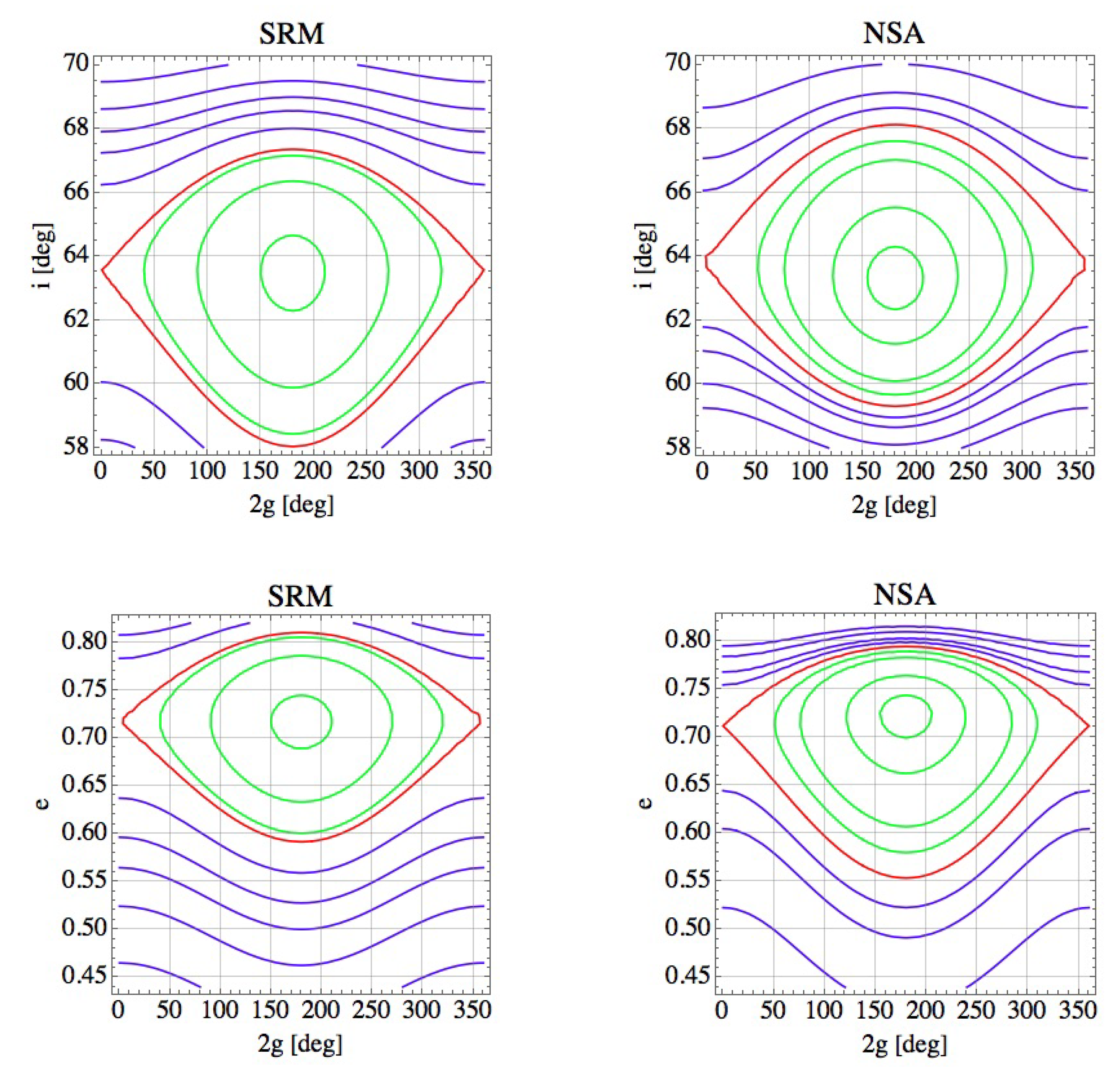
The resonant dominant harmonics for which the SRM gives a reliable description of the phase plane structure are listed in Table 8, while the resonances associated with the arguments in Table 9 exhibit a non-standard behavior. In Table 8, we show the center of libration related to each resonant harmonic and the corresponding maximum width, as computed with the standard approach (SRM) through Equation (23). The maximum real excursion in eccentricity and in inclination, computed by using Equation (26), gives substantially the same width obtained with the SRM. These facts can be appreciated by looking at the phase portraits from Figure 1, Figure 2, Figure 3 and Figure 4. The dynamical structure arising from the pendulum-like Hamiltonian is depicted on the left, while, on the right, we show the results obtained from the resonant Hamiltonian not developed in Taylor series; the Y-axis is always converted in eccentricity or in inclination.
We note that the phase portraits for the cases where the angle does not include the lunar node have been computed considering the contribution of both Sun and Moon. Moreover, since the harmonic argument depending on the lunar ascending node leads to a non-autonomous resonant Hamiltonian, it is necessary to introduce a dummy momentum and a new conjugate angle depending on the lunar node in order to eliminate the explicit linear time dependency. For this reason, there are two first integrals in correspondence of , in Table 8 and Table 9.
The lunisolar periodic component with argument produces a non-negligible contribution to the dynamics of the argument of the pericenter, if compared with the oblateness effect and with the precession due to the lunisolar mean terms. Therefore, the ideal model SRM does not give a reliable estimate of the resonant region, in accordance with [5]. Figure 1 depicts the dynamics in the plane and in the plane around the main resonance. The maximum excursion in inclination, as computed with SRM, is and it is rather similar to the one obtained with NSA in Table 9, the difference being around one degree both for the minimum and the maximum inclination. The excursions in eccentricity given by the two models are instead quite different: the minimum value of the eccentricity reached in the libration region of the pendulum-like approximation is approximately and is quite different from . The maximum values are both above the threshold of 2.
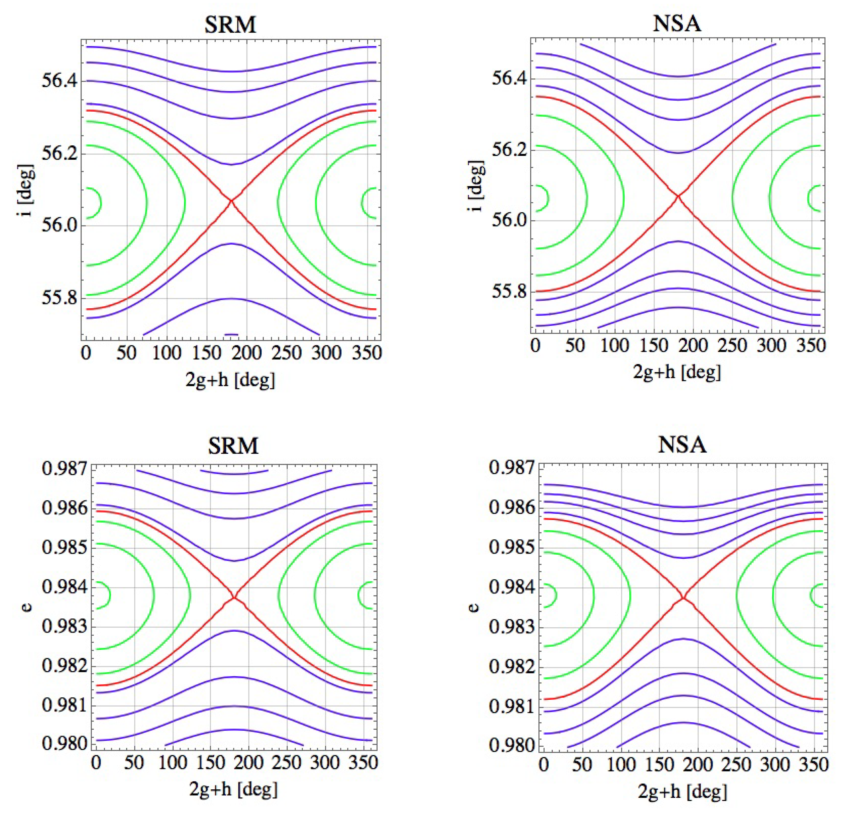
The second dominant term, namely , is not resonant by definition at the critical inclination. By using the Molniya parameters as initial conditions, the equilibrium point lies in the retrograde orbit region, at (see Figure 2).
This means that for a Molniya satellite with , the argument always circulates with a period of approximately years (see Table 5). In any case, the libration region of is quite narrow and does not overlap with the other dynamics taken into account, especially with the main resonance and with , as already pointed out in [5].
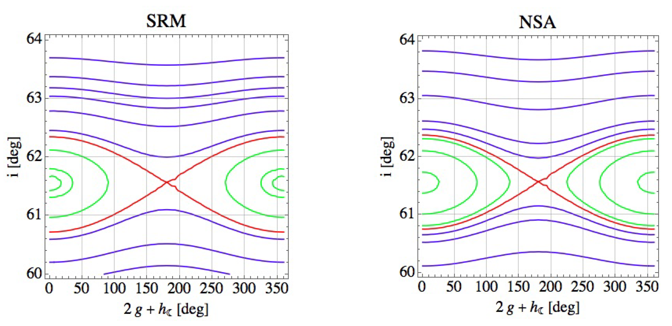
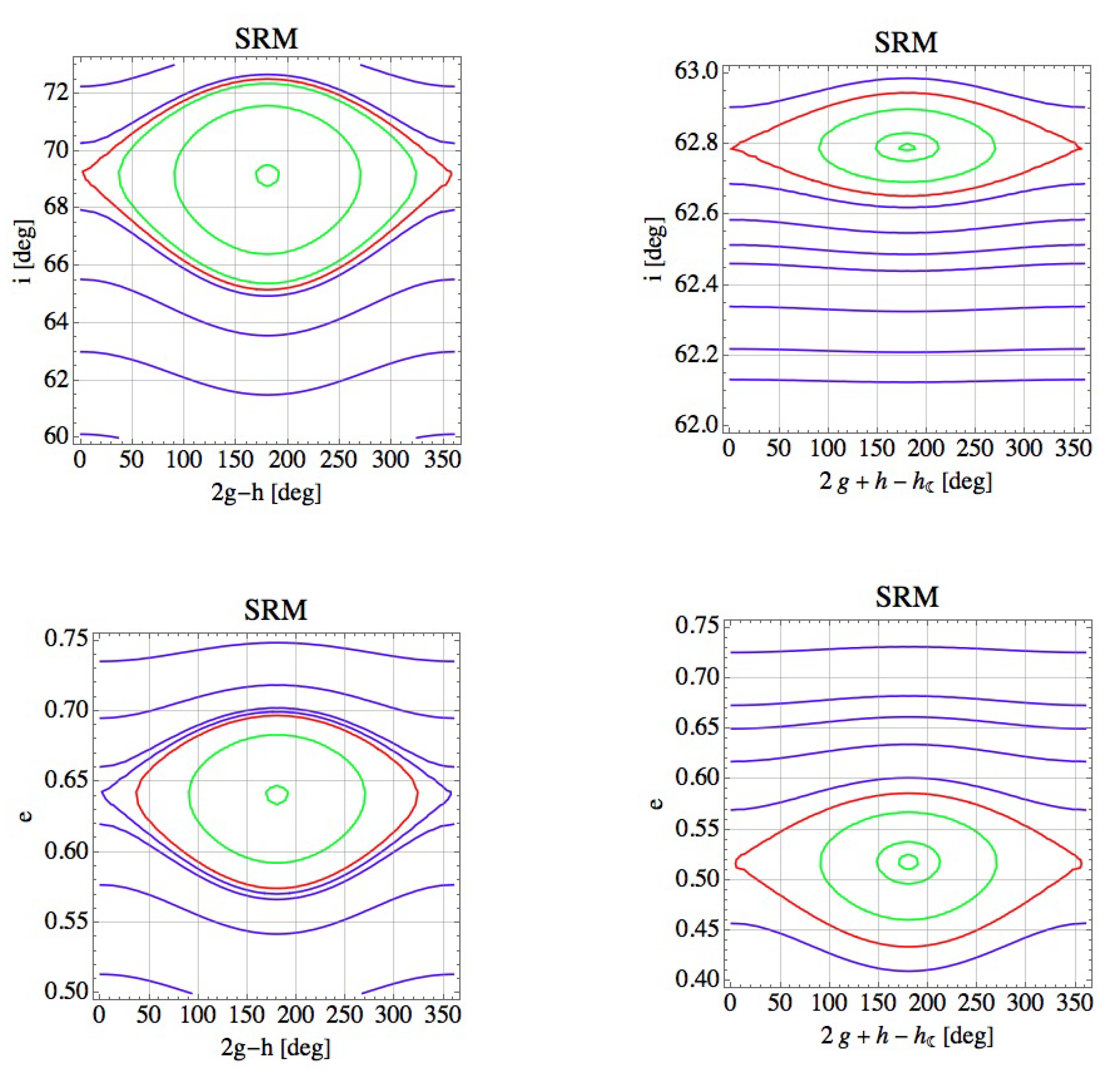
In general, also for the other dominant terms identified (see Figures and Figure 4), the dynamics corresponding to are of circulation, except for the case (Figure ) if we consider a certain tolerance in the inclination, which is reasonable for practical applications [2].
Finally, this analysis shows that initial conditions corresponding to the Molniya parameters allow for a motion in which the width associated with the arguments , , and intersects. By putting together the maximum and the minimum i and e (see Table 8 and Table 9) that may be attained in the libration region of every single resonance, we obtain a maximum overlapping region defined as
that is widely extended both in eccentricity and in inclination. This is depicted in Figure 5, where we display also the resonance , because it takes place in the same domain. In turn, it is not possible to encapsulate the complexity of the Molniya dynamics in a simple way—for instance, with a single-resonance model or a double-resonance model.
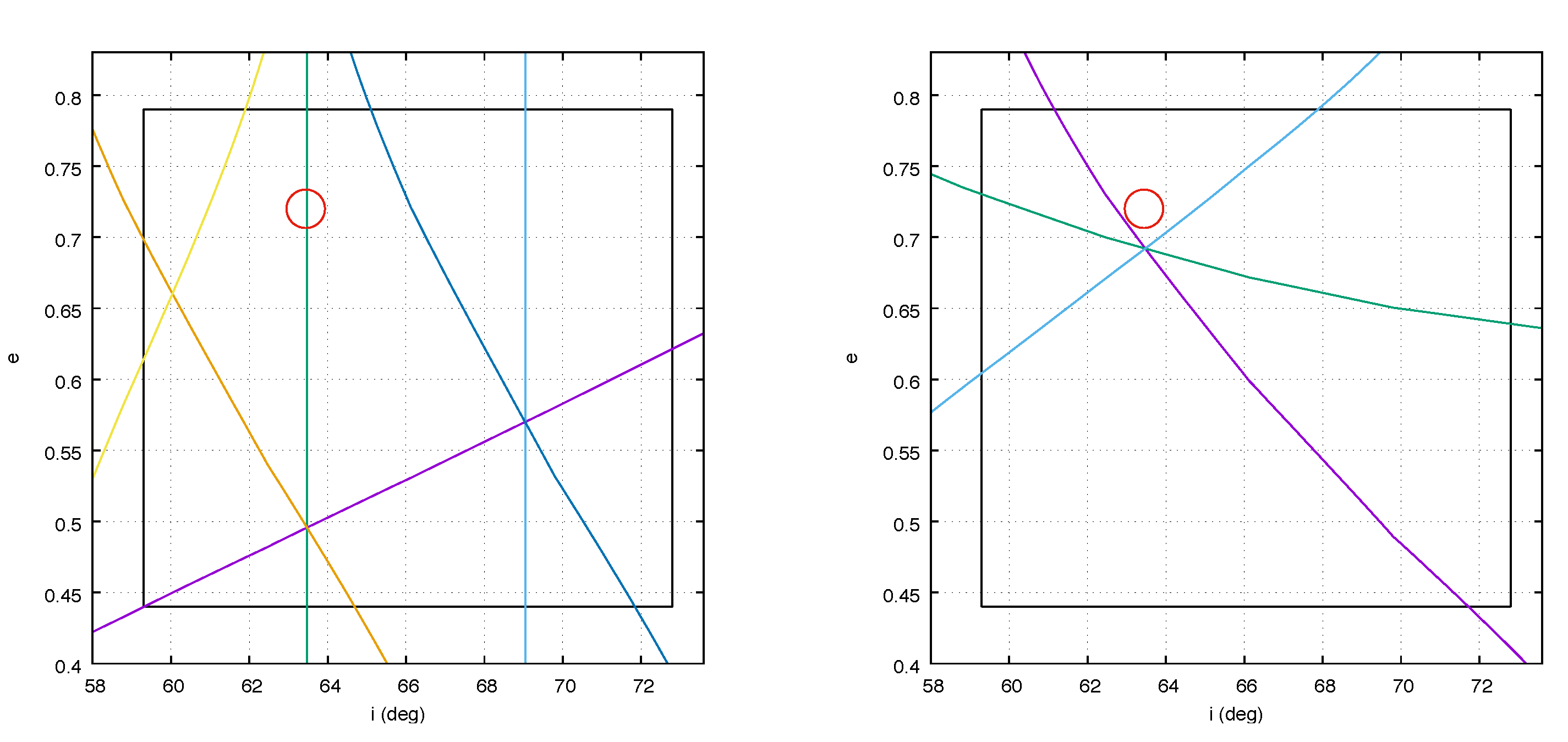
Only three third-order resonances show a ratio larger than a few second-order terms. From Figure 6, which depicts the location of such resonances, we expect that , and occur in the maximum overlapping region found in Equation (28).
5. Conclusions
In this work, we have considered a doubly averaged Hamiltonian model accounting for the Earth’s oblateness effect and the octupolar lunisolar perturbation to estimate the perturbing contribution caused by each term in the specific case of the Molniya satellites’ orbit.
Concerning the evolution of the mean eccentricity and inclination, the role played by the ratio between the harmonic amplitude and the harmonic frequency is crucial to set a “hierarchy” on the large amount of terms that we are dealing with. The analysis provided is general and can be exploited to approach the long-term evolution in other orbital regions. In the case considered here, in addition to the harmonics corresponding to and , considered in the past to be the most important, our investigation shows that the long-term behavior in eccentricity is influenced, at the same level, also by perturbing terms associated with the satellite and the lunar ascending nodes. The amplitude of the second-order dominant terms (beyond ) is at least 1.89 × 10 for the Sun and at least 1.16 × 10 for the Moon. The periods of the most relevant terms are instead: 7.21, 7.55, 7.92, 11.79, 12.71, 16.71 and 21 years. In particular, the terms that exhibit a large ratio are also those identified as the dominant contributors through the numerical experiments given in [2], at least as long as the hypothesis of a constant mean semi-major axis holds. Moreover, we have shown that the third-body effect is crucial also for the evolution of the argument of the pericenter, because of the critical inclination.
Besides providing a robust basis for the choice of the terms to consider in an analytical modeling, a possible application of the analysis is to explain observational data or to estimate the maximum eccentricity growth in the long term due to lunisolar perturbations, as done in [19,20] in the case of solar radiation pressure.
Moreover, in the second part of the paper, we have described the phase space associated with the most important resonant terms causing explicitly an eccentricity variation. We have highlighted in particular when the pendulum-like approach does not give a reliable estimate of the resonance extension. In these cases, the critical inclination characterizing Molniya orbits deforms the lobe of the libration region.
The identification of a maximum overlapping region defined by the main resonant contributions, following the phase space investigation, could be a starting point for the further investigation of a possible chaotic behavior. Finally, the third-order lunisolar perturbation does not seem to be particularly significant as regards the dynamics, but it could play a more important role in relation to chaotic phenomena.
Author Contributions
Conceptualization, T.T., E.M.A. and G.T.; methodology, T.T., E.M.A. and G.T.; software, T.T.; validation, T.T.; formal analysis, T.T.; investigation, T.T.; resources, T.T.; data curation, T.T.; writing—original draft preparation, T.T.; writing—review and editing, E.M.A.; visualization, T.T.; supervision, E.M.A. and G.T. All authors have read and agreed to the published version of the manuscript.
Funding
This research received no external funding.
Institutional Review Board Statement
Not applicable.
Informed Consent Statement
Not applicable.
Data Availability Statement
Not applicable.
Acknowledgments
E.M. Alessi acknowledges the support received from Fondazione Cariplo through the program Promozione dell’attrattività e competitività dei ricercatori su strumenti dell’European Research Council—Sottomisura rafforzamento.
Conflicts of Interest
The authors declare no conflict of interest.
| 1 | We use the following notation to denote the components of a generic vector : where is the canonical basis of . |
| 2 | Molniya orbits with a semi-major axis cannot have an eccentricity larger than because the corresponding perigee altitude would be smaller than the radius of the Earth. |
References
- Wade, M. The Astronautix Web Site. 2019. Available online: http://www.astronautix.com (accessed on 1 December 2021).
- Alessi, E.M.; Buzzoni, A.; Daquin, J.; Carbognani, A.; Tommei, G. Dynamical properties of the Molniya satellites constellation: Long-term evolution of orbital eccentricity. Acta Astronaut. 2021, 179, 659–669. [Google Scholar] [CrossRef]
- Ulybyshev, Y.P. Design of satellite constellations with continuous coverage on elliptic orbits of Molniya type. Cosm. Res. 2009, 47, 310–321. [Google Scholar] [CrossRef]
- Buzzoni, A.; Guichard, J.; Alessi, E.M.; Altavilla, G.; Figer, A.; Carbognani, A.; Tommei, G. Spectrophotometric and dynamical properties of the Soviet/Russian constellation of Molniya satellites. J. Space Saf. Eng. 2020, 7, 255–261. [Google Scholar] [CrossRef]
- Zhu, T.-L.; Zhao, C.-Y.; Wang, H.-B.; Zhang, M.-J. Analysis on the long term orbital evolution of Molniya satellites. Astrophys. Space Sci. 2015, 357, 126. [Google Scholar] [CrossRef]
- McGraw, J.T.; Zimmer, P.C.; Ackermann, M.R. Ever wonder what’s in Molniya? We do. In Proceedings of the Advanced Maui Optical and Space Survelliance (AMOS) Technologies Conference, Maui, HI, USA, 19–22 September 2017; Available online: https://ui.adsabs.harvard.edu/link_gateway/2017amos.confE.107M/PUB_PDF (accessed on 1 December 2021).
- Daquin, J.; Alessi, E.M.; O’Leary, J.; Lemaitre, A.; Buzzoni, A. Dynamical properties of the Molniya satellite constellation: Long-term evolution of the semi-major axis. Nonlinear Dynam. 2021, 105, 2081–2103. [Google Scholar] [CrossRef]
- Ely, T.A.; Howell, K.C. Dynamics of artificial satellite orbits with tesseral resonances including the effects of luni-solar perturbations. Dynam. Stabil. Syst. 1997, 12, 243–269. [Google Scholar] [CrossRef]
- Iorio, L. The Impact of the Static Part of the Earth’s Gravity Field on Some Tests of General Relativity with Satellite Laser Ranging. CMDA 2003, 86, 277–294. [Google Scholar] [CrossRef]
- Murray, C.D.; Dermott, S.F. Solar System Dynamics; Cambridge University Press: Cambridge, UK, 1999. [Google Scholar]
- Colombo, C. Long-term evolution of highly-elliptical orbits: Luni-solar perturbation effect for stability and re-entry. Front. Astron. Space Sci. 2019, 6, 34. [Google Scholar] [CrossRef]
- Celletti, A.; Gales, C.; Pucacco, G.; Rosengren, A.J. Analytical development of lunisolar disturbing function and the critical inclination secular resonance. Celest. Mech. Dyn. Astron. 2017, 127, 259–283. [Google Scholar] [CrossRef] [Green Version]
- Kaula, W.M. Theory of Satellite Geodesy: Applications of Satellites to Geodesy; Blaisdell Publishing Company: Waltham, MA, USA, 1966. [Google Scholar]
- Laskar, J.; Bouè, G. Explicit expansion of the three-body disturbing function for arbitrary eccentricities and inclinations. Astron. Astrophys. 2010, 522, A60. [Google Scholar] [CrossRef]
- Battin, R.H. An Introduction to the Mathematics and Methods of Astrodynamics Revised Edition; AIAA Education Series; American Institute of Aeronautics and Astronautics, Inc.: Reston, VA, USA, 1999. [Google Scholar]
- Morbidelli, A. Modern Celestial Mechanics: Aspects of Solar System Dynamics; Taylor and Francis: London, UK, 2002. [Google Scholar]
- Tremaine, S.; Touma, J.; Namouri, F. Satellite dynamics on the Laplace surface. Astron. J. 2009, 137, 3706–3717. [Google Scholar] [CrossRef]
- Anselmo, L.; Pardini, C. Long-Term Simulation of Object in High-Earth Orbits. ESA/ESOC Study Note. 2006. Available online: https://openportal.isti.cnr.it/doc?id=people______::20ae9d19d50be310fa9fd4910857578f (accessed on 1 December 2021).
- Alessi, E.M.; Schettino, G.; Rossi, A.; Valsecchi, G.B. Solar radiation pressure resonances in Low Earth Orbits. Mon. Not. R. Astron. Soc. 2018, 473, 2407–2414. [Google Scholar] [CrossRef] [Green Version]
- Schettino, G.; Alessi, E.M.; Rossi, A.; Valsecchi, G.B. A frequency portrait of Low Earth Orbits. Celest. Mech. Dyn. Astron. 2019, 131, 35. [Google Scholar] [CrossRef] [Green Version]
Figure 1.
Phase space associated with the dynamics. Contour plot of the pendulum-like approximation (plot title SRM on the left) and of the resonant Hamiltonian not developed in Taylor series (plot title NSA on the right). The X-axis always shows the critical angle in degrees. The Y-axis is converted in inclination (on the top), and measured in degrees, or in eccentricity (on the bottom). Green lines denote the librating curves around the stable equilibrium, purple lines denote the circulation region, while the separatrices are depicted in red.

Figure 2.
Phase space associated with the dynamics. Contour plot of the pendulum-like approximation (SRM on the left) and of the resonant Hamiltonian not developed in Taylor series (NSA on the right). The X-axis always shows the critical angle in degrees. The Y-axis is converted in i (on the top), and measured in degrees, or in e (on the bottom). Green lines denote the librating curves around the stable equilibrium, purple lines denote the circulation region, while the separatrices are depicted in red.

Figure 3.
Phase space associated with the dynamics. Contour plot of the pendulum-like approximation (plot title SRM on the left) and of the resonant Hamiltonian not developed in Taylor series (plot title NSA on the right). The X-axis always shows the critical angle in degrees. The Y-axis is converted in inclination (on the top), and measured in degrees, or in eccentricity (on the bottom). Green lines denote the librating curves around the stable equilibrium, purple lines denote the circulation region, while the separatrices are depicted in red.


Figure 4.
Phase space associated with the and (right) dynamics. The X-axis always shows the critical angle in degrees. The Y-axis is converted in i (on the top), and measured in degrees, or in e (on the bottom). Green lines denote the librating curves around the stable equilibrium, purple lines denote the circulation region, while the separatrices are depicted in red.

Figure 5.
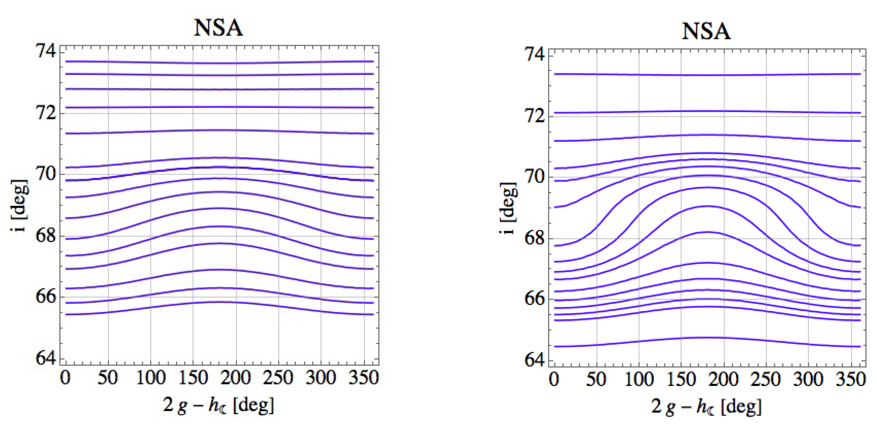
Phase space associated with the dynamics. Contour plot of the Hamiltonian obtained after performing the suitable coordinate change. The pictures show how the phase structure changes by using different initial conditions to evaluate the first integral; is the initial eccentricity, while the initial inclination varies: (top left), (top right), (bottom left), (bottom right). Equilibria emerge by increasing the orbital inclination. Purple lines identify the circulation orbits. The separatrices arising from the different unstable equilibria are drawn in red and black, while the corresponding librating curves are denoted in magenta and orange, respectively. Cyan lines appear only on the bottom left, where there is no clear distinction between the libration region associated with different pairs of recently emerged equilibria.
Figure 5.
Phase space associated with the dynamics. Contour plot of the Hamiltonian obtained after performing the suitable coordinate change. The pictures show how the phase structure changes by using different initial conditions to evaluate the first integral; is the initial eccentricity, while the initial inclination varies: (top left), (top right), (bottom left), (bottom right). Equilibria emerge by increasing the orbital inclination. Purple lines identify the circulation orbits. The separatrices arising from the different unstable equilibria are drawn in red and black, while the corresponding librating curves are denoted in magenta and orange, respectively. Cyan lines appear only on the bottom left, where there is no clear distinction between the libration region associated with different pairs of recently emerged equilibria.


Figure 6.
Left: in the plane, the second-order resonances that correspond to the dominant terms of Table 7 and that can occur in the maximum overlapping region identified (black box). Purple: ; green: ; cyan: ; orange: ; yellow: ; blue: . Right: the third-order resonances with largest ratio (see Table 7) that can occur in the same neighborhood. In both plots, the red circle denotes the Molniya parameters. Purple: ; green: ; cyan: .


Table 1.
Largest amplitudes (in km2/s2), in absolute value, of the solar harmonic coefficients, together with the corresponding argument (left column). The values are computed by evaluating the harmonic coefficients at the Molniya parameters, i.e., .
Table 1.
Largest amplitudes (in km2/s2), in absolute value, of the solar harmonic coefficients, together with the corresponding argument (left column). The values are computed by evaluating the harmonic coefficients at the Molniya parameters, i.e., .
| , | |
|---|---|
| Mean Term | |
Table 2.
Largest amplitudes (in km2/s2), in absolute value, of the lunar harmonic coefficients, together with the corresponding argument. The values are computed by evaluating the harmonic coefficients at the Molniya parameters.
Table 2.
Largest amplitudes (in km2/s2), in absolute value, of the lunar harmonic coefficients, together with the corresponding argument. The values are computed by evaluating the harmonic coefficients at the Molniya parameters.
| , | |
|---|---|
| h | |
| Mean Term | |
Table 3.
Largest amplitudes (in rad/s), in absolute value, of the partial derivatives of the harmonic coefficients with respect to the actions, together with the corresponding argument. The values are computed by evaluating the terms at the Molniya parameters.
Table 3.
Largest amplitudes (in rad/s), in absolute value, of the partial derivatives of the harmonic coefficients with respect to the actions, together with the corresponding argument. The values are computed by evaluating the terms at the Molniya parameters.
| Mean Term | Mean Term | ||||||
| h | |||||||
| h | |||||||
| Mean Term | |||||||
| Mean Term |
Table 4.
Notation and details of the various approximations of considered in the work. The first column is the notation; the second to the fourth columns show whether a perturbing effect is taken into account (✓) or not (−). The last column reports, where relevant, the fixed value (in degrees) of the initial longitude of the ascending node chosen to compute the approximation of .
| Notation | -Term | Mean Terms | Periodic Terms in Table 3 | |
|---|---|---|---|---|
| ✓ | − | − | Not relevant | |
| ✓ | ✓ | − | Not relevant | |
| ✓ | ✓ | ✓ | 90 | |
| ✓ | ✓ | ✓ | 180 | |
| ✓ | ✓ | ✓ | 0 | |
| ✓ | ✓ | ✓ | 270 |
Table 5.
Largest periods (>7 years) for the lunar and solar arguments appearing in the second-order doubly averaged disturbing potential. The first column helps to identify which third body the arguments belong to. The periods (in years) are computed assuming and following the assumptions listed in Table 4 for , as specified at the top of each column.
| Argument | |||||||
|---|---|---|---|---|---|---|---|
| 9777.54 | 513.68 | 196.72 | 163.76 | 150.31 | 130.27 | ||
| ☾ | 40.25 | 43.47 | 50.34 | 53.07 | 54.65 | 57.89 | |
| ☾ | 40.08 | 40.08 | 40.08 | 40.08 | 40.08 | 40.08 | |
| ☾ | 39.92 | 37.18 | 33.30 | 32.20 | 31.64 | 30.65 | |
| ☾ | 18.65 | 19.31 | 20.56 | 21.00 | 21.24 | 21.71 | |
| ☾ | 18.61 | 18.61 | 18.61 | 18.61 | 18.61 | 18.61 | |
| ☾ | 18.58 | 17.96 | 17.00 | 16.71 | 16.56 | 16.28 | |
| ☾ | 12.73 | 13.03 | 13.58 | 13.78 | 13.88 | 14.08 | |
| ☾ | 12.71 | 12.71 | 12.71 | 12.71 | 12.71 | 12.71 | |
| ☾ | 12.69 | 12.40 | 11.94 | 11.79 | 11.72 | 11.58 | |
| ☾ | 9.31 | 9.47 | 9.77 | 9.87 | 9.92 | 10.02 | |
| ☾ | 9.31 | 9.31 | 9.31 | 9.31 | 9.31 | 9.31 | |
| ☾ | 9.30 | 9.14 | 8.89 | 8.81 | 8.76 | 8.68 | |
| 7.56 | 7.66 | 7.85 | 7.92 | 7.95 | 8.01 | ||
| h | 7.55 | 7.55 | 7.55 | 7.55 | 7.55 | 7.55 | |
| 7.55 | 7.55 | 7.27 | 7.21 | 7.19 | 7.13 |
Table 6.
Largest periods for the lunar and solar arguments appearing in the third-order doubly averaged disturbing potential. The first column helps to identify the third body. The periods (in years) are computed assuming the approximations of listed in Table 4 and .
Table 6.
Largest periods for the lunar and solar arguments appearing in the third-order doubly averaged disturbing potential. The first column helps to identify the third body. The periods (in years) are computed assuming the approximations of listed in Table 4 and .
| Argument | |||||||
|---|---|---|---|---|---|---|---|
| ⊙ | 23,669.36 | 1036.82 | 394.83 | 328.48 | 301.43 | 261.16 | |
| ⊙ | 16,659.31 | 1018.06 | 392.08 | 326.57 | 299.83 | 259.95 | |
| ⊙ | 6919.27 | 343.50 | 131.30 | 109.28 | 100.30 | 86.91 | |
| ⊙ | 6161.37 | 341.41 | 131.00 | 109.07 | 100.12 | 86.78 | |
| ☾ | 184.42 | 367.55 | 488.04 | 279.03 | 227.11 | 168.40 | |
| ☾ | 181.00 | 217.27 | 329.57 | 396.41 | 444.55 | 575.42 | |
| ☾ | 177.71 | 152.69 | 123.19 | 115.89 | 112.33 | 106.23 | |
| ☾ | 174.54 | 117.70 | 75.75 | 67.86 | 64.29 | 58.51 | |
| ☾ | 108.11 | 154.24 | 562.28 | 4104.67 | 1736.91 | 473.80 | |
| ☾ | 106.93 | 118.62 | 145.73 | 157.48 | 164.55 | 179.68 | |
| ☾ | 105.77 | 96.37 | 83.72 | 80.28 | 78.55 | 75.52 | |
| ☾ | 104.64 | 81.15 | 58.72 | 53.87 | 51.59 | 47.80 | |
| ☾ | 52.03 | 60.78 | 85.12 | 97.91 | 106.45 | 127.23 | |
| ☾ | 51.75 | 54.35 | 59.41 | 61.27 | 62.32 | 64.37 | |
| ☾ | 51.48 | 49.15 | 45.63 | 44.59 | 44.05 | 43.08 | |
| ☾ | 51.21 | 44.86 | 34.07 | 37.03 | 35.04 | 32.37 |
Table 7.
Lunisolar harmonics with km2/s. The first column helps to identify the third body; the second one indicates whether the corresponding argument appears in the second- or in the third-order lunisolar potential. The ratioR (in km2/s) is computed by assuming the approximations of listed in Table 4 and .
| l | Argument | |||||||
|---|---|---|---|---|---|---|---|---|
| ☾ | 2 | 879,496.40 | 46,205.55 | 17,695.51 | 14,730.36 | 13,520.88 | 11,718.5 | |
| ⊙ | 2 | 407,137.87 | 21,389.55 | 8191.64 | 6819.00 | 6259.11 | 5424.75 | |
| ☾ | 2 | 526.48 | 533.92 | 547.08 | 551.51 | 553.90 | 558.45 | |
| ☾ | 2 | h | 446.00 | 446.00 | 446.004 | 446.00 | 446.00 | 446.00 |
| ⊙ | 2 | 243.72 | 247.16 | 253.25 | 255.30 | 256.41 | 258.52 | |
| ⊙ | 2 | h | 206.46 | 206.46 | 206.46 | 206.46 | 206.46 | 206.46 |
| ☾ | 2 | 200.75 | 197.99 | 193.47 | 192.05 | 191.29 | 189.89 | |
| ☾ | 2 | 175.79 | 180.01 | 187.69 | 190.33 | 191.78 | 194.54 | |
| ☾ | 2 | 148.84 | 148.84 | 148.84 | 148.84 | 148.84 | 148.84 | |
| ☾ | 2 | 108.85 | 112.73 | 120.00 | 122.58 | 124.00 | 126.75 | |
| ☾ | 2 | 108.44 | 104.85 | 99.25 | 97.56 | 96.67 | 95.06 | |
| ⊙ | 2 | 92.93 | 91.65 | 89.56 | 88.90 | 88.55 | 87.90 | |
| ☾ | 2 | 66.96 | 65.43 | 62.97 | 62.22 | 61.82 | 61.08 | |
| ☾ | 2 | 49.65 | 49.65 | 49.65 | 49.65 | 49.65 | 49.65 | |
| ☾ | 2 | 48.33 | 48.33 | 48.33 | 48.33 | 48.33 | 48.33 | |
| ☾ | 2 | 46.15 | 46.48 | 47.04 | 47.22 | 47.32 | 47.51 | |
| ☾ | 2 | 26.42 | 26.42 | 26.42 | 26.42 | 26.42 | 26.42 | |
| ☾ | 2 | 25.23 | 25.46 | 25.84 | 25.97 | 26.04 | 26.17 | |
| ⊙ | 2 | 22.37 | 22.3 | 22.37 | 22.37 | 22.37 | 22.37 | |
| ⊙ | 2 | 21.36 | 21.51 | 21.77 | 21.86 | 21.91 | 21.99 | |
| ☾ | 2 | 11.92 | 12.88 | 14.91 | 15.72 | 16.19 | 17.15 | |
| ☾ | 2 | 10.85 | 10.96 | 11.15 | 11.21 | 11.24 | 11.31 | |
| ☾ | 2 | 10.07 | 10.07 | 10.07 | 10.07 | 10.07 | 10.07 | |
| ☾ | 2 | 9.19 | 9.19 | 9.19 | 9.19 | 9.19 | 9.19 | |
| ☾ | 2 | 6.72 | 6.68 | 6.60 | 6.58 | 6.56 | 6.54 | |
| ☾ | 3 | 5.65 | 6.60 | 9.24 | 10.63 | 11.56 | 13.82 | |
| ☾ | 3 | 5.32 | 5.58 | 6.10 | 6.29 | 6.40 | 6.61 | |
| ☾ | 3 | 5.29 | 5.05 | 4.69 | 4.58 | 4.53 | 4.43 | |
| ☾ | 2 | 4.51 | 4.21 | 3.77 | 3.64 | 3.58 | 3.47 | |
| ☾ | 2 | 4.14 | 4.10 | 4.03 | 4.01 | 4.00 | 3.98 | |
| ☾ | 2 | 3.85 | 3.85 | 3.85 | 3.85 | 3.85 | 3.85 | |
| ☾ | 2 | 3.68 | 3.64 | 3.59 | 3.57 | 3.57 | 3.56 | |
| ☾ | 2 | 3.67 | 3.72 | 3.79 | 3.82 | 3.83 | 3.86 | |
| ⊙ | 2 | 3.11 | 3.09 | 3.06 | 3.04 | 3.04 | 3.03 | |
| ☾ | 3 | 2.12 | 1.86 | 1.53 | 1.45 | 1.41 | 1.34 | |
| ☾ | 3 | 1.77 | 1.81 | 1.89 | 1.92 | 1.94 | 1.97 | |
| ☾ | 3 | 1.76 | 1.18 | 1.65 | 1.63 | 1.62 | 1.60 | |
| ☾ | 3 | 1.27 | 1.18 | 1.05 | 1.01 | 0.99 | 0.96 | |
| ☾ | 3 | 1.21 | 1.25 | 1.31 | 1.33 | 1.34 | 1.36 | |
| ☾ | 3 | 1.21 | 1.23 | 1.25 | 1.26 | 1.26 | 1.27 | |
| ☾ | 3 | 1.21 | 1.18 | 1.13 | 1.11 | 1.10 | 1.09 | |
| ☾ | 3 | 1.15 | 1.15 | 1.16 | 1.16 | 1.16 | 1.16 | |
| ☾ | 3 | 1.15 | 1.14 | 1.13 | 1.13 | 1.13 | 1.13 |
Table 8.
Resonances whose dynamics are well described by the SRM. The first column identifies the resonances through the critical argument associated with it; the second column shows the first integral arising from the resonant Hamiltonian. is the dummy momentum introduced to add one dimension to the phase space in case of resonances involving the lunar ascending node. The center of libration is given in terms of Keplerian elements: identifies the libration center of the exact resonance while gives the center of libration related to the real resonance. (in km2/s) gives information about the asymmetry of the resonant region. The last two columns show the libration width in terms of e and i; the same values are obtained with the SRM Equation (23) and with NSA Equation (26). The values in inclination are reported in degrees.
| Critical Argument | First Integral | |||||||
|---|---|---|---|---|---|---|---|---|
| 0.64 | 0.64 | 69.14 | 69.03 | 114.41 | 0.13 | 7.3 | ||
| 0.98 | 0.98 | 56.06 | 56.06 | 1.20 | 0.004 | 0.55 | ||
| 0.52 | 0.52 | 62.79 | 62.80 | 337.35 | 0.15 | 0.29 | ||
| 0.76 | 0.76 | 61.56 | 61.55 | 10.27 | 0.03 | 1.63 |
Table 9.
Resonances whose dynamics are not appropriately described by the SRM. The first column identifies the resonance through the associated argument; the second column shows the first integral arising from the resonant Hamiltonian. The equilibria are given in terms of eccentricity and inclination: stable ones, unstable ones. (in km2/s) gives information about the asymmetry of the resonant region. The last two columns show the maximum excursion, in terms of e and i, that may be attained in the libration region as computed with NSA through Equation (26). The values in inclination are reported in degrees. N.E. means “not evaluated”.
| Critical Argument | First Integral | |||||||
|---|---|---|---|---|---|---|---|---|
| 0.72 | 0.71 | 63.29 | 63.69 | 625.10 | ||||
| N.E. |
Publisher’s Note: MDPI stays neutral with regard to jurisdictional claims in published maps and institutional affiliations. |
© 2021 by the authors. Licensee MDPI, Basel, Switzerland. This article is an open access article distributed under the terms and conditions of the Creative Commons Attribution (CC BY) license (https://creativecommons.org/licenses/by/4.0/).
Share and Cite
MDPI and ACS Style
Talu, T.; Alessi, E.M.; Tommei, G. On the Dominant Lunisolar Perturbations for Long-Term Eccentricity Variation: The Case of Molniya Satellite Orbits. Universe 2021, 7, 482. https://0-doi-org.brum.beds.ac.uk/10.3390/universe7120482
AMA Style
Talu T, Alessi EM, Tommei G. On the Dominant Lunisolar Perturbations for Long-Term Eccentricity Variation: The Case of Molniya Satellite Orbits. Universe. 2021; 7(12):482. https://0-doi-org.brum.beds.ac.uk/10.3390/universe7120482
Chicago/Turabian StyleTalu, Tiziana, Elisa Maria Alessi, and Giacomo Tommei. 2021. "On the Dominant Lunisolar Perturbations for Long-Term Eccentricity Variation: The Case of Molniya Satellite Orbits" Universe 7, no. 12: 482. https://0-doi-org.brum.beds.ac.uk/10.3390/universe7120482
Note that from the first issue of 2016, this journal uses article numbers instead of page numbers. See further details here.