Gravitational Lensing of Continuous Gravitational Waves

Abstract

Continuous gravitational waves are analogous to monochromatic light and could therefore be used to detect wave effects such as interference or diffraction. This would be possible with strongly lensed gravitational waves. This article reviews and summarises the theory of gravitational lensing in the context of gravitational waves in two different regimes: geometric optics and wave optics, for two widely used lens models such as the point mass lens and the Singular Isothermal Sphere (SIS). Observable effects due to the wave nature of gravitational waves are discussed. As a consequence of interference, GWs produce beat patterns which might be observable with next generation detectors such as the ground based Einstein Telescope and Cosmic Explorer, or the space-borne LISA and DECIGO. This will provide us with an opportunity to estimate the properties of the lensing system and other cosmological parameters with alternative techniques. Diffractive microlensing could become a valuable method of searching for intermediate mass black holes formed in the centres of globular clusters. We also point to an interesting idea of detecting the Poisson–Arago spot proposed in the literature.

1. Introduction

With the first detection of gravitational waves (GWs) in 2015 from the coalescing compact binary system [1], we have entered the long-expected era of GW astronomy. A new window in the Universe has been opened. First, GW detections brought about the confirmation of the existence of binary black hole (BBH) systems in nature. A half of a century ago, the primary candidates for chirping signals were binary neutron stars (BNS) due to sober expectations based on Hulse–Taylor-like BNS systems discovered so far. Indeed, in 2017, the first of such coalescence was registered [2], and accompanying electromagnetic signals spanning from gamma rays through optical rays and radio waves were registered, allowing for the identification of the host galaxy and making a plethora of various other tests possible. Further observing runs of the LIGO–Virgo–KAGRA network considerably enriched the statistics of registered events. In the future, there will be a qualitative boost when the third generation of ground-based detectors such as the Einstein Telescope (ET) [3] or the Cosmic Explorer (CE) [4] as well as space-borne detectors (LISA, DECIGO, TianQin) [5,6,7,8,9,10] become operative. First, the sensitivity of ground-based detectors will be increased by an order of magnitude over the existing ones, allowing for the exploration of a larger volume of the universe by three orders of magnitude. Second, the satellite detectors will probe much lower frequencies of GWs (inaccessible from the ground due to seismic noise), enabling the observation of adiabatic inspiralling signals from binary systems much earlier than the coalescence phase probed by ground-based detectors. This means that besides the already registered chirp signals, we would gain access to almost monochromatic continuous GW signals.

In this paper we discuss some new opportunities that will be available when continuous GW signals are registered. In the case of light, historically, there has been a dispute about its nature: corpuscular vs. wave. The wave nature of light has been established with interference and diffraction patterns, which are best visible with monochromatic light. By analogy, interference and diffraction patterns should be revealed in GWs as well. But what sort of experiment could be performed in this context? We point to gravitationally lensed GW signals as a promising physical setting to reveal the wave effects of GWs. The first ideas of this kind were formulated by [11,12], where the proper treatment of this phenomenon within the wave regime was presented.

The bending of light by the sun was the first classic test of general relativity. The essence of light bending by massive bodies lies in the fact that paths of photons (light rays) are null geodesics in spacetime, which is curved by the presence of mass. Since Eddington’s expedition in 1919, this phenomenon has now evolved to a mature discipline of extragalactic astronomy called gravitational lensing. Currently, this is routinely used to study the structure of galaxies (lenses) and in cosmology. Gravitational waves, in the geometric optics approximation, follow the null geodesics as well. Hence, one can expect to see gravitationally lensed GW signals. Such signals coming from unresolved images would interfere, producing characteristic patterns. In the next section, we will review the strong lensing of GWs. Section 3 contains a discussion of some observable effects that are particularly pronounced when the source emits continuous GWs. We summarise the article in Section 4.

2. Gravitational Lensing of Gravitational Waves

As one of the successful predictions of general relativity, strong gravitational lensing by galaxies has become one of the most important tools in studying cosmology [13], galaxy structure, and evolution [14]. With the dawn of gravitational wave astronomy, the robust prediction suggested that a considerable number of GW signals from inspiralling neutron stars would be gravitationally lensed, and detected by third-generation, ground-based GW detectors [15] or the planned space-based GW detectors LISA [16] and DECIGO [17].

2.1. Strong Gravitational Lensing in Brief

Strong gravitational lensing occurs whenever the source, the lens (a galaxy, a black hole, a star), and the observer are almost aligned. In the particular case of perfect alignment, the source will not be obscured by the lens but will instead be made visible as a glowing ring—also known as the Einstein ring. In the case of axisymmetric lenses, the angular radius of this ring, i.e., the Einstein radius, is the following:

$${\theta }_E=\sqrt{\frac{4G{M}_l}{c^2}\frac{D_{ls}}{D_l{D}_s}},$$

(1)

where $D_l$ is the angular diameter distance to the lens at redshift $z_l$, $D_s$ is the angular diameter distance to the source at redshift $z_s$, $D_{ls}$ is the angular diameter distance between the lens and the source. $M_l$ is the total projected mass of the lens contained within the Einstein radius $M(r<{\theta }_E)$. For the point mass (or a very compact object), it is just the total mass of the lens. Misalignment in this optical system by the angle $\beta$ (angle between directions to the source and to the lens) leads to the appearance of multiple images. Usually, two or four images (with a spherically symmetric mass distribution) are formed at angular separations of ${\theta }_i$ from the center of the lens. The typical separation between different images is set by the Einstein radius, and their locations are described by the following lens equation:

$$\beta =\theta -\alpha \left(\theta \right)$$

(2)

where $\alpha \left(\theta \right)$ is the deflection angle determined by the projected mass distribution of the lens (for detailed derivations, see [18]). The total time delay introduced by gravitational lensing at the angular position $\theta$ from the lens is calculated as follows:

$$\Delta t=\frac{1+z_l}{c}\frac{D_l{D}_s}{D_{ls}}\left[\frac{{(\theta -\beta )}^2}{2}-\varphi \left(\theta \right)+{\varphi }_m\left(\beta \right)\right]$$

(3)

where $\varphi \left(\theta \right)$ is the lens potential determining the deflection angle $\alpha \left(\theta \right)={\nabla }_{\theta }\varphi \left(\theta \right)$. Term ${\varphi }_m\left(\beta \right)$ corresponds to the arrival time in a non-lensed case, and in practice, it is a constant adjusted to ensure the extreme value of the time delay functional. Total time delay, or more precisely the time delay functional, measures the delay between lensed signal arrival from the image at position $\theta$ with respect to the (unmeasurable) arrival time from the source if the lens was absent. Fermat’s principle implies that images correspond to stationary points of the time delay functional, and one can see that condition ${\nabla }_{\theta }\Delta t=0$ is equivalent to the lens Equation (2). The measurable quantity is the time delay difference $\Delta t_{ij}$ between images at ${\theta }_i$ and ${\theta }_j$. Another measurable quantity is the ratio of image magnifications. The (signed) magnification is the inverse Jacobian of the lens equation: $\mu ={\left(det\left(\frac{\partial \beta }{\partial \theta }\right)\right)}^{-1}$. The sign corresponds to the parity of the image, so $\left|\mu \right|$ is physically relevant, and since the intrinsic luminosity is usually unknown, only magnification ratios are relevant. The exception could be the lensed standard candles, where the absolute magnification could be derived. In the optical system, image locations are another sort of observables, but in the case of GWs, they are irrelevant.

For the purpose of this work, we refer to two of the simplest and most commonly used analytic lens models: the point mass model and the singular isothermal sphere (SIS) model. Their choice is dictated by two realistic scenarios: lensing by an isolated mass such as a massive (with $M_l<{10}^7{M}_{\odot }$) black hole (BH) or an intervening galaxy ($M_l$∼${10}^9$–${10}^{11}{M}_{\odot }$).

In the case of axisymmetric point lenses, the typical separation between different images is set by the Einstein radius (1). The dimensionless lens Equation (2) and its corresponding solutions are as follows [18]:

$$y=x-\frac{1}{x}\to \begin{array}{c}\left\{\begin{array}{c}{x}_{+}=\frac{y+\sqrt{y^2+4}}{2}\\ x_{-}=\frac{y-\sqrt{y^2+4}}{2}\end{array}\right.\end{array}$$

(4)

where $y=\beta /{\theta }_E$, and $x=\theta /{\theta }_E$. Hence, two images could be produced at angular positions ${\theta }_{+}=x_{+}{\theta }_E$ and ${\theta }_{-}=x_{-}{\theta }_E$, respectively. The magnification of images reads as follows:

$${\mu }_{\pm }={\left[1-{\left(\frac{1}{x_{\pm }}\right)}^4\right]}^{-1}.$$

(5)

The time delay between images produced by a point mass lens is calculated with the following equation [18]:

$$\Delta t=\frac{4G{M}_l(1+z_l)}{c^3}\left(\frac{y\sqrt{y^2+4}}{2}+ln\frac{\sqrt{y^2+4}+y}{\sqrt{y^2+4}-y}\right).$$

(6)

Point mass lenses (also called Schwarzschild lenses) are representative of lensing by stars (microlensing) and BHs with stellar or intermediate mass BHs.

It has been well-established that early type galaxies act as lenses in the majority of the strongly gravitational lens systems detected. Even though their formation and evolution are still not fully understood in detail, a singular isothermal sphere model (SIS) can reasonably characterize the mass distribution of massive elliptical galaxies within the effective radius [14,19,20,21]. In the case of the axisymmetric SIS model [22,23], its three-dimensional density profile could be described as $\rho \left(r\right)={\sigma }_v^2/2\pi G{r}^2$, where r is the distance from the sphere center and ${\sigma }_v$ is the velocity dispersion of the lens. In this case, the dimensionless lens Equation (2) could be written as follows [18]:

$$y=x-\frac{x}{\left|x\right|},$$

(7)

where $x=\theta /{\theta }_E$, $y=\beta /{\theta }_E$, as above. When $y<1$, the solutions are:

$$x_{\pm }=y\pm 1.$$

(8)

The corresponding angular positions of the images are ${\theta }_{\pm }=\beta \pm {\theta }_E$, where:

$${\theta }_E=4\pi \frac{{\sigma }_v^2}{c^2}\frac{D_{ls}}{D_s}.$$

(9)

In this case, the magnifications of the images are the following:

$${\mu }_{\pm }=1\pm \frac{1}{y}.$$

(10)

On the other hand, when $y>1$, the lens equation only has one solution: $x=y+1$. Its corresponding magnification is $\mu =\left|x\right|/\left(\left|x\right|-1\right)$.

For the SIS model, the time delay between different images reads as follows:

$$\Delta t=\frac{32{\pi }^2}{c}{\left(\frac{{\sigma }_v}{c}\right)}^4\frac{D_l{D}_{ls}}{D_s}(1+z_l)y.$$

(11)

2.2. Wave Optics Regime

The above summarised results were obtained using the geometric optics approximation, which is excellent in most astrophysically relevant cases of the strong gravitational lensing of electromagnetic waves. Indeed, this approximation is valid as long as the typical length scale of the system is much larger than the wavelength, and the timescale of the typical variations of the system are much larger than the period of the wave. In the case of GWs, things become different: the frequency range probed by ground-based detectors comprise 10 Hz $<f<10$ kHz (to be lowered down to 1 Hz in the future third generation), while in the space-borne detectors, it will be 0.1 mHz $<f<100$ mHz for LISA and 1 mHz $<f<100$ Hz for DECIGO. This corresponds to the GW wavelengths of ${10}^4$ m $<\lambda <{10}^7$ m in ground-based and ${10}^6$ m $<\lambda <{10}^{12}$ m in space-borne detectors.

In the wave optics regime, we consider the gravitational wave from a distant source as propagating in the background spacetime $g_{\mu \nu }^{\left(L\right)}$ of the lens object characterized by the gravitational potential $U\left(\mathbf{r}\right)<<1$. The total metric, including the perturbation (due to the GW signal) is given by $g_{\mu \nu }=g_{\mu \nu }^{\left(L\right)}+h_{\mu \nu }$, where $h_{\mu \nu }=\psi e_{\mu \nu }$. Since the polarization tensor $e_{\mu \nu }$ is parallel transported along the null geodesic, we may neglect its change (being of order $\sim U\left(\mathbf{r}\right)<<1$) and study the propagation equation of the scalar wave: ${\partial }_{\mu }\left(\sqrt{-g^{\left(L\right)}}{g}^{\left(L\right)\mu \nu }{\partial }_{\nu }\psi \right)=0$. For the monochromatic scalar wave $\psi (\mathbf{r},t)=\tilde{\psi }(\mathbf{r})e^{-2\pi ift}$ in the frequency domain, and remembering the weak potential assumption, this equation can be cast to the form of the Helmholtz equation:

$$\left({\nabla }^2+4{\pi }^2{f}^2\right)\tilde{\psi }=16{\pi }^2{f}^{2}U\tilde{\psi }$$

(12)

The solution to the Helmholtz equation can be given in terms of the Kirchhoff integral [18], where it is convenient to introduce the dimensionless amplification factor:

$$F\left(f\right)=\frac{{\tilde{\psi }}^L}{\tilde{\psi }}$$

(13)

which is the ratio of wave amplitudes with and without lensing. Then, the Kirchhoff integral allows us to calculate the amplification factor at the observer [18] as:

$$F(f,\beta )=\frac{1+z_l}{c}\frac{D_s}{D_l{D}_{ls}}\frac{f}{i}\int d^2\theta exp\left[2\pi if\Delta t(\theta ,\beta )\right]$$

(14)

where $\Delta t$ is the lensing time delay given by Equation (3), and the cosmological nature of distances in the optical system has been taken into account. The calculation of the integral (14) can be simplified by switching from angles to dimensionless variables x and y (see above after Equation (5)) and by introducing the new parameter $w=\frac{8\pi G}{c^3}{M}_l\left({\theta }_E\right)(1+z_l)f$:

$$F(w,y)=\frac{w}{2\pi i}\int d^{2}y\left[exp\left[iwT\right(x,y)\right]$$

(15)

where $T(x,y)=\frac{{(x-y)}^2}{2}-\frac{\varphi \left(x\right)}{{\theta }_E^2}$. In general, the amplification factor (15) should be evaluated numerically, but in two particular cases, it can be integrated analytically. In the point mass lens model, the dimensionless lensing potential is $\varphi \left(\mathbf{x}\right)=lnx$, and the analytical solution to the diffraction integral is given by the following equation:

$$F\left(f\right)=exp\left[\frac{\pi w}{4}+i\frac{w}{2}\left(ln\left(\frac{w}{2}\right)-2{\varphi }_m\left(y\right)\right)\right]\Gamma \left(1-\frac{i}{2}w\right){}_1{F}_1\left(\frac{i}{2}w,1;w{y}^2\right)$$

(16)

where ${\varphi }_m\left(y\right)=0.5{(x_m-y)}^2/2-ln{x}_m$ with $x_m=(y+\sqrt{y^2+4})/2$, and ${}_1{F}_1$ is the confluent hypergeometric function.

In the case of the SIS model, the Kirchhoff integral could be cast into an analytically manageable form [12]:

$$F\left(f\right)=-iw{e}^{iw{y}^2/2}{\int }_0^{\infty }dxx{J}_0\left(wxy\right)exp\left[iw\left(\frac{1}{2}{x}^2-x+{\varphi }_m\left(y\right)\right)\right]$$

(17)

where ${\varphi }_m\left(y\right)=y+1/2$ and the $J_0$ is the Bessel function of order zero.

Geometric optics formally corresponds to $f\to \infty$; hence, $w>>1$. In such a case, the Kirchhoff integral can be calculated by using stationary phase approximation, and dominant contributions will come from image positions. Hence, the amplification of the wave intensity is as follows:

$${\left|F\left(f\right)\right|}^2=|{\mu }_{+}{|}^2+|{\mu }_{-}{|}^2+2\left|{\mu }_{+}{\mu }_{-}\right|sin(2\pi f\Delta t_d)$$

(18)

where the first two terms correspond to magnifications in geometric optics, and the last one represents the interference between images.

3. Effects of the Gravitational Wave Lensing of Continuous Waves

Since the lensed images would not be resolved, they are expected to come from the same location in the sky, separated in time by the lensing time delay $\Delta t_{ij}$. In the case of coalescences of compact binary systems, these are expected to be revealed as just two signals with similar temporal patterns and amplitudes affected by magnification. This picture is basically true for merging systems staying within the detectors’ sensitivity band for a fraction of a second. However, if such a system could be monitored earlier, i.e., in the adiabatic inspiral phase (an almost monochromatic signal), then the brighter image (arriving earlier) could imprint its interference patterns on the strain of the fainter image. In this section, we will discuss some of these effects stemming from the wave nature of GWs, which could be observed. Here, we will review some fresh ideas that have already appeared in the literature (and to which one of us contributed).

3.1. Beat Patterns

An interesting paper [24] discussed that if the lensed images from the coalescing binary system could be detected simultaneously by the detector, then beat patterns would be revealed prior to the merger signal. The merger signal would arrive first from the brighter (more magnified) image, then the merger signal from the fainter one would be registered after lensing time delay. If they stayed for a couple of seconds in the detector sensitivity band, then one would see beat patterns. First of all, this condition is very restrictive for the strong lensing system configuration: time delay should be of order of minutes at most. This means that the probability of detecting such an event from the ground is much lower than the probability of detecting a strong lensed GW in general. However, the payoff of such a detection should be considerable because, as the authors of [24] argue, one would be able to measure the redshifted lens mass purely from the GW signal and measure the time delay distance without reconstructing the Fermat potential. This is interesting enough, and it is thus worth recalling the basic points here.

Suppose that we have a signal in time domain $h\left(t\right)$, which is a superposition of two differently magnified signals from two unresolved images:

$$\begin{array}{cc}h\hfill & ={\mu }_{+}[A^{+}cos({\omega }_{1}t+{\varphi }_1)+A^{\times }sin({\omega }_{1}t+{\varphi }_1)]+\hfill \\ \hfill & +{\mu }_{-}[A^{+}cos({\omega }_{2}t+{\varphi }_2)+A^{\times }sin({\omega }_{2}t+{\varphi }_2)]\hfill \end{array}$$

(19)

where ${\mu }_{+}$ and ${\mu }_{-}$ are their respective magnification, $A^{+}$ and $A^{\times }$ are the amplitudes, and ${\omega }_1$,${\omega }_2$,${\varphi }_1$,${\varphi }_2$ are angular frequencies and initial phases, respectively. These can be rewritten as follows:

$$\begin{array}{cc}h\hfill & ={\mu }_{sum}\left[A^{+}cos({\omega }_{f}t+{\varphi }_f)cos({\omega }_{b}t+{\varphi }_b)+A^{\times }sin({\omega }_{f}t+{\varphi }_f)cos({\omega }_{b}t+{\varphi }_b)\right]+\hfill \\ \hfill & +{\mu }_{diff}\left[-A^{+}sin({\omega }_{f}t+{\varphi }_f)sin({\omega }_{b}t+{\varphi }_b)+A^{\times }cos({\omega }_{f}t+{\varphi }_f)sin({\omega }_{b}t+{\varphi }_b)\right]\hfill \end{array}$$

(20)

with ${\mu }_{sum}={\mu }_{+}+{\mu }_{-},$${\mu }_{diff}={\mu }_{+}-{\mu }_{-},$ the frequencies ${\omega }_b=\frac{{\omega }_1-{\omega }_2}{2}$ and ${\omega }_f=\frac{{\omega }_1+{\omega }_2}{2}$ represent the beat and the average frequency, respectively, and phases ${\varphi }_b,{\varphi }_f$ are defined in a similar manner. In the early inspiral phase (i.e., well before coalescence), when the frequency evolves according to $\frac{d\omega }{dt}=\frac{192}{5}{\mathcal{M}}^{5/3}{\left(\frac{\omega }{2}\right)}^{11/3}$ [25,26] and ${\omega }_b<<{\omega }_f\approx {\omega }_1\approx {\omega }_2$, one has the following:

$${\omega }_b=\frac{96}{5}{\left(\frac{{\omega }_f}{2}\right)}^{11/3}\mathcal{M}\Delta t$$

(21)

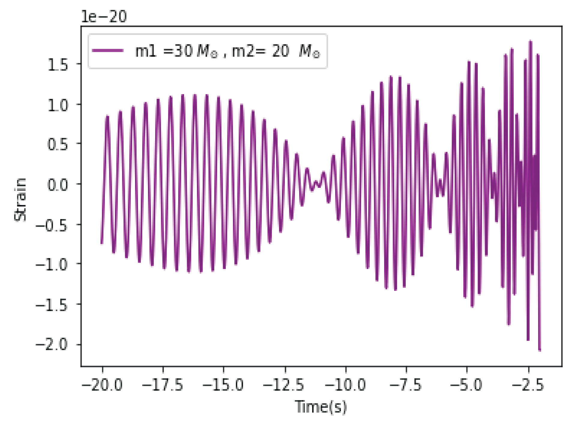
where $\mathcal{M}$ is the chirp mass of the binary system and $\Delta t$ is the lensing time delay (3) given by formula (6) in the case of the point mass lens. Figure 1 illustrates the beat pattern originating in the lensed coalescing system. One can see the evolution of the beat pattern toward the coalescence. During the last stages of the inspiral phase, ${\omega }_f$ increases and the beat pattern disappears. In the case of the lensed continuous GW signals, the beat pattern would be rigid. Now, if one uses the beat pattern defined by Equation (20) as a template in the matched filtering method, then the ratio $\frac{{\mu }_{sum}}{{\mu }_{diff}}$ can be extracted from the data and easily converted to the magnification ratio $r=\left|\frac{{\mu }_{+}}{{\mu }_{-}}\right|$. The lensing time delay $\Delta t$ is directly measurable, and in the case of registering two coalescence signals, the accuracy of such a measurement would be unprecedented. In the case of almost monochromatic signals from the inspiral phase long before the merger (accessible in low-frequency bands of DECIGO and LISA), the time delay $\Delta t$ could still be extracted from the matched filtering using the beat pattern template. The knowledge of the magnification ratio r will allow for interesting inferences to be made. In the case of a point mass lens, after expressing the time delay (6) in terms of r, one can see that the redshifted mass of the lens can be calculated as follows:

$$M_l(1+z_l)=\frac{c^3}{2G}\Delta t{\left[\frac{r-1}{\sqrt{r}}+lnr\right]}^{-1}$$

(22)

On the other hand, in the case of the SIS lens, the so-called time delay distance $D_{\Delta t}$ can be obtained with the following equation:

$$D_{\Delta t}\equiv \frac{D_l{D}_{ls}}{D_s}=\frac{c^5\Delta t}{32{\pi }^2{\sigma }_v^4(1+z_l)}\frac{r-1}{r+1}$$

(23)

provided that the lens is identified and its redshift is known. This is also an important result, demonstrating the breadth of information which can be extracted from the GW signal alone. Needless to say, time delay distance measurements have been used to determine the Hubble constant in a way that is independent of the cosmic ladder or CMB techniques. It has been shown in [27] that lensed GW signals from coalescing BNS systems would allow for a percent accuracy in $H_0$ measurements. Moreover, the time delay distance can be used to test the cosmological model beyond the $\Lambda$CDM.

Given the promising applications of beat patterns, a natural question arises concerning their detectability. In order to forecast the yearly rate of lensed GW signals from compact binary systems, one usually assumes that both images, the faint one and the bright one, should have an SNR above the threshold. From the perspective of beat patterns, an additional demand is that time delays should be comparable to the time spent in the sensitivity band of the detector. These factors modify the optical depth appropriately. Such a self-consistent study of beat patterns detectability has been performed for the planned DECIGO and B-DECIGO missions [24]. For the Einstein Telescope, there has been a series of studies focused on the lensed GW signals in general. The initial one assumed that sources should intrinsically have an SNR greater than or equal to the detection threshold [28]. Then, this demand was relaxed in [15], updating the forecasts for intrinsically faint signals, which could be registered because of magnification due to lensing. Then, the rotation of the Earth was taken into account in [29] since it influences the detector’s orientation factors for the signals separated by the lensing time delay. Robust predictions for the Einstein Telescope are 50–100 lensed GW signals per year. Finally, the newest study [30] considered the third generation of detectors in a network configuration with existing detectors and applied realistic signal templates for the study. The conclusion was that a more realistic scenario improves the detection rate. However, beat pattern detectability puts restrictions on the time delay, so the results of these studies cannot be easily carried over. A dedicated study is necessary. Let us also comment on the following issue. Namely, that the Einstein Telescope is expected to register 10${}^5$–10${}^6$ BBH coalescences per year. This means that optimistically ET would detect one such coalescence every minute. Whether such frequent chirping events occurring simultaneously for some time before the merger would produce interference patterns is an interesting question to be studied further.

3.2. Diffractive Microlensing

Besides the strong lensing discussed in the previous section, which in the case of an electromagnetic window usually means multiple images of a quasar (or galaxy) lensed by a galaxy, one can consider microlensing. It is again a strong lensing case (usually starlight lensed by a star) where the images cannot be resolved, but the relative motion of the elements of the optical system make the temporal changes in the total magnification of the source detectable. It was an ingenious idea of Paczyński [31] that two individually unobservable effects (image separation and relative proper motion) can be combined to give an observable effect. One can expect that the similar phenomenon could be detected in the GW domain. In the paper [32], such a setting was proposed and discussed. In addition to [32], fringes due to GW lensing were also studied in [33,34,35].

One can think of the gravitational lensing of GWs (in or close to the wave regime) as an analogue of a one-slit or two-slit experiment with light. When the light is monochromatic (such as a laser beam), a characteristic fringe pattern is visible on the screen. In astrophysical scales, the “screen” has astronomical scales and is inaccessible directly. This corresponds to a fixed y parameter. However, in the microlensing case, y changes in time (due to relative motions) and one can explore the “screen” by watching the manifestation of fringes. The peculiar motions of the lensing system mentioned above include the motion of the observer ${\mathbf{v}}_{obs}$, the source ${\mathbf{v}}_s$, and the lens ${\mathbf{v}}_l$—all measured in the CMB frame combined to obtain the effective velocity ${\mathbf{v}}_{eff}$ as given by the following equation [36]:

$${\mathbf{v}}_{eff}={\mathbf{v}}_s-\frac{1+z_s}{1+z_l}\frac{D_s}{D_l}{\mathbf{v}}_l+\frac{1+z_s}{1+z_l}\frac{D_{ls}}{D_l}{\mathbf{v}}_{obs}$$

(24)

In lensing, since we are referring to angles in the sky, the effective velocity should be converted to angular proper motion.

For the comparison between the size of the “barrier” (lens) and the wavelength of the GW, one uses the parameter $w=\frac{8\pi G}{c^3}{M}_l\left({\theta }_E\right)(1+z_l)f$ introduced in Section 2. Recall that if $w>>1$, the amplification factor in (14) simplifies to (18). The last term in (18) is the interference term. If the amplitude of the diffraction fringes are to be detectable, the parameter w should be large enough (but not too big). It has been proposed in [32] that $w>1$ is the reasonable condition for the fringe pattern to be detectable. To see a complete diffraction or interference pattern, the observation period $T_{obs}$ should be more than the timescale over which the fringe pattern is affected due to the peculiar motion of the system; we then denote the fringe timescale as $t_f$. This timescale of the transit of fringes can be denoted by $t_f=\frac{t_E}{w}$, where $t_E$ is the Einstein radius crossing time. For galactic sources and lens, it is given by the equation below:

$$t_E\approx 34.7\mathrm{days}\sqrt{4\frac{D_l}{D_s}\left(1-\frac{D_l}{D_s}\right)}{\left(\frac{D_s}{8\mathrm{kpc}}\right)}^{1/2}\times {\left(\frac{M}{M_{\odot }}\right)}^{1/2}{\left(\frac{{\mathbf{v}}_{eff}}{200\mathrm{km}{\mathrm{s}}^{-1}}\right)}^{-1}$$

(25)

Therefore, the criterion for detecting a fringe pattern can be summarised in three conditions [32]:

• w > 1, to have enough amplification;
• y < 3, to detect fringes before they are damped;
• $\Delta t>t_f$, to see a fringe pattern.

Let us say that the second condition means that the probability of microlensing is almost an order of magnitude larger than that of the optical. It is because the cross-section for lensing is proportional to the Einstein ring area $\pi y^2$, and in the optical, $y=1$ is the threshold for microlensing.

Estimates of [37,38] suggest that a galactic bulge contains about ${10}^9$ NSs and a globular cluster contains ${10}^3$ NSs, which could be the target population for the current and next-generation gravitational detectors. In order to find the probability of observing a fringe pattern from such a population of monochromatic sources, one would need to calculate the optical depth, which gives the probability that a given source falls into the Einstein radius of any lens located along the line of sight $\tau ={\int }_0^{D_s}n\left(D_l\right)\pi R_E^{2}d{D}_l.$ If we consider a source population in the Milky Way bulge lensed by a constant density of stellar mass lenses in the galactic disc moving with a velocity $v_{rot}=200{\mathrm{kms}}^{-1}$, the lensing probability is given by the following equation [31,39]:

$$\tau =\frac{v_{rot}^2}{2c^2}=f_l\times {10}^{-6}$$

(26)

where $f_l$ is the fraction of the lens larger than one solar mass, which is required to fulfil the above-mentioned conditions for diffractive microlensing.

Currently, the issue of intermediate mass BHs and their existence has been debated. They can be formed in the very cores of globular clusters. Therefore, it would be interesting to focus on globular clusters as the hosts of gravitational lenses for lensing continuous GWs. One such candidate is already known. M22 is a rich globular cluster with a projected location pointing to the Galactic bulge—a perfect site of sources (spinning neutron stars or binary systems). A typical velocity dispersion in a globular cluster is ${\sigma }_v$∼10 km s${}^{-1}$; hence, the typical transverse velocity of the lens can be very well approximated by that of a cluster as a whole ∼200 km s${}^{-1}$. Once again, ref. [40] showed that the optical depth for microlensing in such a case is:

$$\tau =f_l\frac{{\sigma }^2}{c^2}\frac{2\pi }{\phi }\frac{D_{ls}}{D_s}\approx 2.4{10}^{-4}{f}_l{\left(\frac{{\sigma }_v}{10\mathrm{km}{\mathrm{s}}^{-1}}\right)}^2\left(\frac{1^{\prime }}{\phi }\right)\frac{D_{ls}}{D_s}$$

(27)

where $\phi$ denotes the angular distance from the center of the cluster. Knowledge of the distance and the transversal velocity of the lenses belonging to the cluster may result in accurate estimates of their masses, breaking the degeneracies inherent to the microlensing technique. The microlensing of the bulge star at $D_s=8.2$ kpc by a low-mass object in the globular cluster M22 located at $D_l=2.6$ has been reported in [41]. Let us remark that the inclusion of the $\phi$ term was motivated by the fact that in the optical system, only the outskirts of the cluster can produce the microlensing of the bulge stars. Regions close to the center would obscure the light of bulge stars. In the GW domain, this is completely different—GWs can easily probe central parts of the cluster. This will significantly enhance the optical depth. Moreover, the intermediate mass black holes (IMBHs) M∼10${}^2$–${10}^4{M}_{\odot }$ are expected to reside in the centres of globular clusters. Hence, diffractive microlensing could open a new chapter in the search for IMBHs. One of the candidates among continuous GW signals is a (slightly deformed) spinning neutron star. Their detection is fairly difficult since the signal is strongly modulated by the Earth’s rotation and orbital motion. Moreover, this modulation is different for every sky position. Diffraction and interference fringes caused by an intervening mass acting as a lens and moving with respect to the source also produce modulation. Luckily, the timescales of these effects are significantly different from timescales involved in the motion of the detector. In the setting we have discussed here, the directed search with the known position in the sky (in the case of globular cluster lensing) can be applied. The GW signal coming from a rotating NS is so weak that in order to detect it in the detector’s noise, one has to analyse months-long segments of data. The implementation of the F-statistic [25] (or G-statistics [42]) consists of coherent searches over two-day periods, and it is followed by a search for coincidences among the candidates from the two-day segments. The timescales for fringe modulation are larger, and one can expect that respective amplitude modulation could be detectable with current techniques. In order to be able to make any rigorous statements, further research on mock data involving real data analysis tools is required. One may hope that this approach should be extended to other sources of continuous GWs such as binary systems that are observable in low-frequency bands to be probed by DECIGO and LISA. This, however, also demands dedicated studies.

3.3. Poisson–Arago Spot

One of the observable signatures of the wave nature of light, besides interference, is diffraction. The French physicist, Fresnel, presented his work on diffraction in a competition sponsored by the French Academy of Sciences in 1818. It was a period when Newton’s idea of the corpuscular theory of light was prevalent. One of the judges in the competition, Poisson, in an attempt to disprove the wave nature of light, pointed out that according to Fresnel’s theory, a parallel beam of light falling on a spherical obstacle would produce a bright spot at the centre, as if the obstacle were not present. This was considered to be an absurd result. Later, another French physicist, Arago, successfully conducted an experiment, and the Poisson spot was seen. This phenomenon later came to be known as Poisson’s spot or the Spot of Arago, which established the wave nature of light in the 19th century. Therefore, a similar phenomenon should be expected of GWs, and a strong lensing optical configuration appears to be the perfect candidate. The reason for the appearance of the spot is that wavefronts originating at the boundary of a circular obstacle interfere constructively. The same is expected from the Einstein ring of lensed GW. To some extent, one can see analogous behaviour in the wave GW regime, when the amplification calculated from the Kirchhoff integral (15) has a maximal value, when $\beta =0$ [43]:

$${\left|F(w,\beta =0)\right|}^2=\frac{\pi w}{1-e^{-\pi w}}.$$

(28)

An interesting and rigorous study of the Poisson–Arago spot that was produced when GWs were passing in the background of a Schwarzschild BH was presented in [44]. This strong-field scenario can be understood as an on-axis scattering problem using the Regge–Wheeler equation [45,46], which describes the axial perturbations of the Schwarzschild metric as a linear approximation [47], and the solutions are given by the confluent Heun equation. The amplitude of the gravitational wave passing in the background of this opaque disc is given by the following equation:

$${\Phi }_l=\frac{1}{r}\sum _{l=2}^{\infty }(2l+1)e^{-i\omega t}{P}_l(cos\theta )R_{ls}\left(r\right)$$

(29)

where $P_l(cos\theta )$ denotes the Legendre polynomials and $R_{ls}$ is the $l-th$ partial wave of the GW, with the spin $s=2$ and the angular momentum $\hslash \sqrt{l(l+1)}$ measured with respect to the scattering centre. For a Schwarzschild BH, the gravitational waves with the impact parameters $3\sqrt{3}M$ fall into the black hole and will not reach infinity, i.e., BH can shield the gravitational waves. $R_{ls}/r$ in (29) is an oscillatory function in the far zone, at which the summation in l in Equation (29) becomes divergent. This issue can be solved in [48] by using the Fresnel half-wave zone, according to which an effective contribution to diffraction comes from the 1/4 zone, and the residues cancel each other. In the case of a small scattering angle and at a large distance, $R_{ls}/r$ becomes:

$${\Phi }_l=e^{-i\omega t}{e}^{\omega r(1-\frac{{\theta }^2}{4})+\pi M\omega }\Gamma (1-2i\omega M)J_0\left(2\sqrt{\frac{M}{r}\omega r\theta }\right)$$

(30)

The fringe pattern is determined by the function $J_0\left(2\sqrt{\frac{M}{r}\omega r\theta }\right)$. The time delay between successive bright or dark spots depends on the mass of the BH, the wavelength of the gravitational wave, and the relative position of the system. The upper bound of the wavelength is set by the radius of the opaque disc. For the supermassive black hole in our galaxy of the radius $6\times {10}^{10}$ m, this corresponds to the frequency of $f=0.005$ Hz. This is within the sensitivity band of the planned space-based detectors such as LISA and TianQin. There is no theoretical lower limit in this calculation; a realistic lower bound depends on the sensitivity of the gravitational wave detector. For a gravitational wave at a frequency of 100 Hz, with SMBH in our galaxy as an obstacle, the diffraction time delay between the bright spot and the first dark fringe is 3.86 days, while that for the second bright fringe is 6.2 days. These effects will be observable with a sensitive ground-based detector.

4. Conclusions

The gravitational lensing of GW signals has been discussed in many papers since its first detection [48]. In particular, [49] put forward an idea that unexpectedly high masses of BBHs detected by LIGO are consequences of the signals being lensed. These claims have been subsequently refuted [50], but the interest in lensed GW remained. Some teams have undertaken efforts to monitor ongoing LIGO–Vrigo–KAGRA detections for the possibility of some signals being lensed by galaxy clusters [51] and with the hope of repeating the Refsdal supernova story [52].

In this paper, we have discussed new opportunities for detecting wave effects in lensed GW signals such as beat patterns (interference) and diffractive microlensing. The former would allow for an independent measurement of the lens mass and the time-delay distance purely from the GW signal. The latter would open a new opportunity to search for IMBHs inside globular clusters and more generally, study the central parts of globular clusters—a technique completely inaccessible through the electromagnetic window. Lensing in the geometrical optics regime preserves the waveform, while the wave diffraction induces amplitude and phase modulation in the frequency domain waveform. The emerging opportunities to detect dark matter clumps at cosmological distances has been discussed in [53]. The authors developed a dynamic programming-based algorithm to search for amplitude and phase modulations imprinted in the waveform due to diffractive lensing. The algorithm does not require a template bank for lensed waveforms, and its feasibility has been demonstrated in simulated mock data. A more recent study, which delineated the regime where wave effects are significant from the regime where geometric effects are significant, was performed in [54]. For a detailed study on the effects of the microlens population in galaxy scale lenses within the LIGO/VIRGO frequency band (10–10${}^4$ Hz), we refer the reader to [55]. Moreover, microlensing is affected by different parameters such as stellar densities, distribution of microlens population around the source, Initial Mass Function (IMF), and types of images [55].

The future third-generation detectors, such as the Einstein Telescope [3] or the Cosmic Explorer [4], are expected to detect lensed GW signals routinely at the rate of 50–100 events per year [28,29]. The prospects are also bright for the planned space-borne detectors such as DECIGO, which will probe a volume of the Universe an order of magnitude larger than the ET. In [17], it has been estimated that DECIGO would routinely register about 50 lensed GW signals per year. Remarkably, some of these sources will later enter the band of ground-based detectors. Inspiralling sources detectable with the DECIGO would exhibit slowly evolving frequency, hence being almost monochromatic and allowing for the detection of patterns discussed in this paper. The expected rate of detecting beat patterns by DECIGO was assessed in [56]. All the studies performed so far regrading lensed GW signals in the wave regime have been focused on high frequency GWs detectable from the ground. Such analyses involving mock data simulations should be extended to low frequencies to be probed by DECIGO, LISA, and TianQin.

Finally, let us comment on the issue of non-linear GWs. Usually, gravitational waves are studied in the weak-field approximation of the Einstein equations in vacuum. Thus, with this limit, they evolve as linear waves. However, gravitational waves are intrinsically non-linear, and both cylindrical and planar nonlinear GWs can be interpreted as soliton solutions to the Einstein equations. For more recent discussions of non-linear GWs, see [57]. With the gravitational lensing of such waves, their interference or diffraction would result in interesting phenomenology, certainly worth investigating in the future.

References

- Abbott, B.P.; Abbott, R.; Abbott, T.D.; Abernathy, M.R.; Acernese, F.; Ackley, K.; Adams, C.; Adams, T.; Addesso, P.; Adhikari, R.X.; et al. Observation of Gravitational Waves from a Binary Black Hole Merger. Phys. Rev. Lett. 2016, 116, 061102. [Google Scholar] [CrossRef] [PubMed]
- Abbott, B.P.; Abbott, R.; Abbott, T.D.; Acernese, F.; Ackley, K.; Adams, C.; Adams, T.; Addesso, P.; Adhikari, R.X.; Adya, V.B.; et al. GW170817: Observation of Gravitational Waves from a Binary Neutron Star Inspiral. Phys. Rev. Lett. 2017, 119, 161101. [Google Scholar] [CrossRef] [PubMed] [Green Version]
- Punturo, M.; Abernathy, M.; Acernese, F.; Allen, B.; Andersson, N.; Arun, K.; Barone, F.; Barr, B.; Barsuglia, M.; Beker, M.; et al. The Einstein Telescope: A third-generation gravitational wave observatory. Class. Quant. Grav. 2010, 27, 194002. [Google Scholar] [CrossRef]
- Dwyer, S.; Sigg, D.; Ballmer, S.W.; Barsotti, L.; Mavalvala, N.; Evans, M. Gravitational wave detector with cosmological reach. Phys. Rev. D 2015, 91, 082001. [Google Scholar] [CrossRef] [Green Version]
- Danzmann, K.; for the LISA Study Team. LISA—An ESA cornerstone mission for a gravitational wave observatory. Class. Quant. Grav. 1997, 14, 1399–1404. [Google Scholar] [CrossRef]
- Amaro-Seoane, P.; Audley, H.; Babak, S.; Baker, J.; Barausse, E.; Bender, P.; Berti, E.; Binetruy, P.; Born, M.; Bortoluzzi, D.; et al. Laser Interferometer Space Antenna. arXiv 2017, arXiv:1702.00786. [Google Scholar]
- Seto, N.; Kawamura, S.; Nakamura, T. Possibility of Direct Measurement of the Acceleration of the Universe Using 0.1 Hz Band Laser Interferometer Gravitational Wave Antenna in Space. Phys. Rev. Lett. 2001, 87, 221103. [Google Scholar] [CrossRef]
- Kawamura, S.; Nakamura, T.; Ando, M.; Seto, N.; Tsubono, K.; Numata, K.; Takahashi, R.; Nagano, S.; Ishikawa, T.; Musha, M.; et al. The Japanese space gravitational wave antenna—DECIGO. Class. Quant. Grav. 2006, 23, S125–S131. [Google Scholar] [CrossRef]
- Kawamura, S.; Ando, M.; Seto, N.; Sato, S.; Nakamura, T.; Tsubono, K.; Kanda, N.; Tanaka, T.; Yokoyama, J.; Funaki, I.; et al. The Japanese space gravitational wave antenna: DECIGO. Class. Quant. Grav. 2011, 28, 094011. [Google Scholar] [CrossRef]
- Gong, Y.; Luo, J.; Wang, B. Concepts and status of Chinese space gravitational wave detection projects. Nat. Astron. 2021, 5, 881–889. [Google Scholar] [CrossRef]
- Nakamura, T.T. Gravitational Lensing of Gravitational Waves from Inspiraling Binaries by a Point Mass Lens. Phys. Rev. Lett. 1998, 80, 1138–1141. [Google Scholar] [CrossRef]
- Takahashi, R.; Nakamura, T. Wave Effects in the Gravitational Lensing of Gravitational Waves from Chirping Binaries. Astrophys. J. 2003, 595, 1039–1051. [Google Scholar] [CrossRef] [Green Version]
- Cao, S.; Biesiada, M.; Gavazzi, R.; Piórkowska, A.; Zhu, Z.H. Cosmology with strong-lensing systems. Astrophys. J. 2015, 806, 185. [Google Scholar] [CrossRef]
- Cao, S.; Biesiada, M.; Yao, M.; Zhu, Z.H. Limits on the power-law mass and luminosity density profiles of elliptical galaxies from gravitational lensing systems. MNRAS 2016, 461, 2192–2199. [Google Scholar] [CrossRef] [Green Version]
- Ding, X.; Biesiada, M.; Zhu, Z.H. Strongly lensed gravitational waves from intrinsically faint double compact binaries—Prediction for the Einstein Telescope. J. Cosmol. Astropart. Phys. 2015, 2015, 006. [Google Scholar] [CrossRef] [Green Version]
- Sereno, M.; Sesana, A.; Bleuler, A.; Jetzer, P.; Volonteri, M.; Begelman, M.C. Strong Lensing of Gravitational Waves as Seen by LISA. Phys. Rev. Lett. 2010, 105, 251101. [Google Scholar] [CrossRef] [Green Version]
- Piórkowska-Kurpas, A.; Hou, S.; Biesiada, M.; Ding, X.; Cao, S.; Fan, X.; Kawamura, S.; Zhu, Z.H. Inspiraling Double Compact Object Detection and Lensing Rate: Forecast for DECIGO and B-DECIGO. Astrophys. J. 2021, 908, 196. [Google Scholar] [CrossRef]
- Schneider, P.; Ehlers, J.; Falco, E.E. Gravitational Lenses; Springer: Berlin/Heidelberg, Germany, 1992. [Google Scholar] [CrossRef]
- Treu, T.; Koopmans, L.V.E. Massive Dark Matter Halos and Evolution of Early-Type Galaxies toz≈1. Astrophys. J. 2004, 611, 739–760. [Google Scholar] [CrossRef] [Green Version]
- Treu, T.; Koopmans, L.V.E.; Bolton, A.S.; Burles, S.; Moustakas, L.A. Erratum: “The Sloan Lens ACS Survey. II. Stellar Populations and Internal Structure of Early-Type Lens Galaxies” (ApJ, 640, 662 [2006]). Astrophys. J. 2006, 650, 1219. [Google Scholar] [CrossRef]
- Liu, T.; Cao, S.; Zhang, J.; Biesiada, M.; Liu, Y.; Lian, Y. Testing the cosmic curvature at high redshifts: The combination of LSST strong lensing systems and quasars as new standard candles. Mon. Not. R. Astron. Soc. 2020, 496, 708–717. [Google Scholar] [CrossRef]
- Narayan, R.; Bartelmann, M. Lectures on Gravitational Lensing. arXiv 1996, arXiv:astro–ph/9606001. [Google Scholar]
- Bernardeau, F. Gravitation lenses. In Theoretical and Observational Cosmology; NATO Advanced Study Institute (ASI) Series C; Lachièze-Rey, M., Ed.; Springer-Science+Business Media: Dordrecht, The Netherlands, 1999; Volume 541, p. 179. [Google Scholar]
- Hou, S.; Fan, X.L.; Liao, K.; Zhu, Z.H. Gravitational wave interference via gravitational lensing: Measurements of luminosity distance, lens mass, and cosmological parameters. Phys. Rev. D 2020, 101, 064011. [Google Scholar] [CrossRef] [Green Version]
- Jaranowski, P.; Krolak, A. Analysis of Gravitational-Wave Data. Cambridge University Press: Cambridge, UK, 2009. [Google Scholar]
- Maggiore, M. Gravitational Waves. Volume 1: Theory and Experiments; Oxford University Press: New York, NY, USA, 2007; ISBN 978-0-19-857074-5. [Google Scholar] [CrossRef]
- Liao, K.; Fan, X.L.; Ding, X.; Biesiada, M.; Zhu, Z.H. Precision cosmology from future lensed gravitational wave and electromagnetic signals. Nat. Commun. 2017, 8, 1148. [Google Scholar] [CrossRef] [PubMed]
- Biesiada, M.; Ding, X.; Piórkowska, A.; Zhu, Z.H. Strong gravitational lensing of gravitational waves from double compact binaries—Perspectives for the Einstein Telescope. J. Cosmol. Astropart. Phys. 2014, 2014, 80. [Google Scholar] [CrossRef] [Green Version]
- Yang, L.; Ding, X.; Biesiada, M.; Liao, K.; Zhu, Z.H. How Does the Earth’s Rotation Affect Predictions of Gravitational Wave Strong Lensing Rates? Astrophys. J. 2019, 874, 139. [Google Scholar] [CrossRef]
- Yang, L.; Wu, S.; Liao, K.; Ding, X.; You, Z.; Cao, Z.; Biesiada, M.; Zhu, Z.H. Event rate predictions of strongly lensed gravitational waves with detector networks and more realistic templates. Mon. Not. R. Astron. Soc. 2021, 509, 3772–3778. [Google Scholar] [CrossRef]
- Paczynski, B. Gravitational Microlensing by the Galactic Halo. Astrophys. J. 1986, 304, 1. [Google Scholar] [CrossRef]
- Liao, K.; Biesiada, M.; Fan, X.L. The Wave Nature of Continuous Gravitational Waves from Microlensing. Astrophys. J. 2019, 875, 139. [Google Scholar] [CrossRef]
- Lai, K.H.; Hannuksela, O.A.; Herrera-Martín, A.; Diego, J.M.; Broadhurst, T.; Li, T.G.F. Discovering intermediate-mass black hole lenses through gravitational wave lensing. Phys. Rev. D 2018, 98, 083005. [Google Scholar] [CrossRef] [Green Version]
- Jung, S.; Shin, C.S. Gravitational-Wave Fringes at LIGO: Detecting Compact Dark Matter by Gravitational Lensing. Phys. Rev. Lett. 2019, 122, 041103. [Google Scholar] [CrossRef] [Green Version]
- Christian, P.; Vitale, S.; Loeb, A. Detecting stellar lensing of gravitational waves with ground-based observatories. Phys. Rev. D 2018, 98, 103022. [Google Scholar] [CrossRef] [Green Version]
- Kayser, R.; Refsdal, S.; Stabell, R. Astrophysical applications of gravitational micro-lensing. Astron. Astrophys. 1986, 166, 36–52. [Google Scholar]
- Narayan, R.; Ostriker, J.P. Pulsar Populations and Their Evolution. Astrophys. J. 1990, 352, 222. [Google Scholar] [CrossRef]
- Arnett, W.D.; Schramm, D.N.; Truran, J.W. On Relative Supernova Rates and Nucleosynthesis Roles. Astrophys. J. 1989, 339, L25. [Google Scholar] [CrossRef]
- Paczynski, B. Gravitational Microlensing of the Galactic Bulge Stars. Astrophys. J. 1991, 371, L63. [Google Scholar] [CrossRef]
- Paczynski, B. Gravitational Microlensing by the Globular Cluster Stars. Acta Astron. 1994, 44, 235–239. [Google Scholar]
- Pietrukowicz, P.; Minniti, D.; Jetzer, P.; Alonso-García, J.; Udalski, A. The first confirmed microlens in a globular cluster. Astrophys. J. Lett. 2011, 744, L18. [Google Scholar] [CrossRef] [Green Version]
- Jaranowski, P.; Królak, A. Searching for gravitational waves from known pulsars using the and statistics. Class. Quant. Grav. 2010, 27, 194015. [Google Scholar] [CrossRef]
- Oguri, M. Strong gravitational lensing of explosive transients. Rep. Prog. Phys. 2019, 82, 126901. [Google Scholar] [CrossRef] [Green Version]
- Zhang, H.; Fan, X. Poisson-Arago spot for gravitational waves. Sci. China Phys. Mech. Astron. 2021, 64, 120462. [Google Scholar] [CrossRef]
- Regge, T.; Wheeler, J.A. Stability of a Schwarzschild Singularity. Phys. Rev. 1957, 108, 1063–1069. [Google Scholar] [CrossRef]
- Nambu, Y.; Noda, S.; Sakai, Y. Wave optics in spacetimes with compact gravitating object. Phys. Rev. D 2019, 100, 064037. [Google Scholar] [CrossRef] [Green Version]
- Fiziev, P.P. Exact solutions of Regge–Wheeler equation and quasi-normal modes of compact objects. Class. Quant. Grav. 2006, 23, 2447–2468. [Google Scholar] [CrossRef] [Green Version]
- Ng, K.K.Y.; Wong, K.W.K.; Broadhurst, T.; Li, T.G.F. Precise LIGO lensing rate predictions for binary black holes. Phys. Rev. D 2018, 97, 023012. [Google Scholar] [CrossRef] [Green Version]
- Broadhurst, T.; Diego, J.M.; Smoot, G.F., III. Twin LIGO/Virgo Detections of a Viable Gravitationally-Lensed Black Hole Merger. arXiv 2019, arXiv:1901.03190. [Google Scholar]
- Abbott, R.; Abbott, T.D.; Abraham, S.; Acernese, F.; Ackley, K.; Adams, A.; Adams, C.; Adhikari, R.X.; Adya, V.B.; Affeldt, C.; et al. Search for lensing signatures in the gravitational-wave observations from the first half of LIGO-Virgo’s third observing run. arXiv 2021, arXiv:2105.06384. [Google Scholar] [CrossRef]
- Smith, G.P.; Berry, C.; Bianconi, M.; Farr, W.M.; Jauzac, M.; Massey, R.; Richard, J.; Robertson, A.; Sharon, K.; Vecchio, A.; et al. Strong-lensing of Gravitational Waves by Galaxy Clusters. Proc. Int. Astron. Union 2017, 13, 98–102. [Google Scholar] [CrossRef] [Green Version]
- Kelly, P.L.; Rodney, S.A.; Treu, T.; Strolger, L.G.; Foley, R.J.; Jha, S.W.; Selsing, J.; Brammer, G.; Bradač, M.; Cenko, S.B.; et al. Deja vu all over again: The reappearance of supernova refsdal. Astrophys. J. 2016, 819, L8. [Google Scholar] [CrossRef] [Green Version]
- Dai, L.; Li, S.S.; Zackay, B.; Mao, S.; Lu, Y. Detecting lensing-induced diffraction in astrophysical gravitational waves. Phys. Rev. D 2018, 98, 104029. [Google Scholar] [CrossRef] [Green Version]
- Meena, A.K.; Bagla, J.S. Gravitational lensing of gravitational waves: Wave nature and prospects for detection. Mon. Not. R. Astron. Soc. 2019, 492, 1127–1134. [Google Scholar] [CrossRef] [Green Version]
- Mishra, A.; Meena, A.K.; More, A.; Bose, S.; Bagla, J.S. Gravitational lensing of gravitational waves: Effect of microlens population in lensing galaxies. Mon. Not. R. Astron. Soc. 2021, 508, 4869–4886. [Google Scholar] [CrossRef]
- Hou, S.; Li, P.; Yu, H.; Biesiada, M.; Fan, X.L.; Kawamura, S.; Zhu, Z.H. Lensing rates of gravitational wave signals displaying beat patterns detectable by DECIGO and B-DECIGO. Phys. Rev. D 2021, 103, 044005. [Google Scholar] [CrossRef]
- Villatoro, F.R. Nonlinear Gravitational Waves and Solitons. In Nonlinear Systems, Vol. 1: Mathematical Theory and Computational Methods; Carmona, V., Cuevas-Maraver, J., Fernández-Sánchez, F., García-Medina, E., Eds.; Springer International Publishing: Cham, Switzerland, 2018; pp. 207–240. [Google Scholar] [CrossRef]
Figure 1.
A diagram showing the beat pattern of a binary inspiral signal. Masses of the components are and , the source is located at , the lens at is assumed to be a point mass of Time delay has been chosen as , thus fixing the parameter.
Publisher’s Note: MDPI stays neutral with regard to jurisdictional claims in published maps and institutional affiliations. |
© 2021 by the authors. Licensee MDPI, Basel, Switzerland. This article is an open access article distributed under the terms and conditions of the Creative Commons Attribution (CC BY) license (https://creativecommons.org/licenses/by/4.0/).
Share and Cite
MDPI and ACS Style
Biesiada, M.; Harikumar, S. Gravitational Lensing of Continuous Gravitational Waves. Universe 2021, 7, 502. https://0-doi-org.brum.beds.ac.uk/10.3390/universe7120502
AMA Style
Biesiada M, Harikumar S. Gravitational Lensing of Continuous Gravitational Waves. Universe. 2021; 7(12):502. https://0-doi-org.brum.beds.ac.uk/10.3390/universe7120502
Chicago/Turabian StyleBiesiada, Marek, and Sreekanth Harikumar. 2021. "Gravitational Lensing of Continuous Gravitational Waves" Universe 7, no. 12: 502. https://0-doi-org.brum.beds.ac.uk/10.3390/universe7120502
Note that from the first issue of 2016, this journal uses article numbers instead of page numbers. See further details here.