
The Dipolar Solar Minimum Corona


National Institute for Astrophysics, Astrophysical Observatory of Torino, Via Osservatorio 20, I-10025 Pino Torinese, Italy
Universe 2021, 7(12), 507; https://0-doi-org.brum.beds.ac.uk/10.3390/universe7120507
Submission received: 24 November 2021
/
Revised: 7 December 2021
/
Accepted: 18 December 2021
/
Published: 20 December 2021
(This article belongs to the Special Issue Advances in Solar Wind Origin and Evolution)
Abstract
:The large-scale configuration of the UV solar corona at the minimum activity between solar cycles 22 and 23 is explored in this paper. Exploiting a large sample of spectroscopic observations acquired by the Ultraviolet Coronagraph Spectrometer aboard the Solar and Heliospheric Observatory in the two-year period of 1996–1997, this work provides the first-ever monochromatic O vi 1032 Å image of the extended corona, and the first-ever two-dimensional maps of the kinetic temperature of oxygen ions and the O vi Å doublet intensity ratio (a proxy for the outflow velocity of the oxygen component of the solar wind), statistically representative of solar minimum conditions. A clear dipolar magnetic structure, both equator- and axis-symmetric, is distinctly shown to shape the solar minimum corona, both in UV emission and in temperature and expansion rate. This statistical approach allows for robust establishment of the key role played by the magnetic field divergence in modulating the speed and temperature of the coronal flows, and identification of the coronal sources of the fast and slow solar wind.
1. Introduction
The solar corona is the outermost layer of the Sun’s atmosphere. It is the region where the plasma is heated to such high temperatures that it is much hotter than the underlying solar surface in such a seemingly paradoxical fashion [1]. It is also where the solar wind, a continuous stream of charged particles, originates and is accelerated to supersonic speeds, then expanding into the heliosphere, the Sun’s region of influence that permeates the whole solar system and a bit beyond, interacting with the planets’ magnetospheres [2]. The solar corona and the solar wind, so closely related to each other, represent a fascinating puzzle whose unraveling is crucial for the solar and plasma physics community. However, other various fields, such as space weather and planetary habitability science, which strongly depend on the interplay of processes between the planet, stellar wind and host star, would greatly benefit from a deep understanding of the solar corona-solar wind coupled system (e.g., [3,4,5,6,7,8,9]). Outstanding questions concern the formation of the solar wind, the physical mechanisms at the base of the plasma heating, the origin, evolution and dissipation of Alfvén waves and turbulence (two basic ingredients of the solar wind), as well as the transport of energetic particles in the heliosphere [10]. It is therefore not surprising that some of the most important solar missions of the space exploration era have been focusing on the observation of the solar corona by means of remote sensing instruments, as well as on in situ measurements of the local properties of the solar wind since the Mariner 2 spacecraft, during its journey to Venus, first established empirically its existence [11], which Parker had theoretically predicted just 4 years earlier in 1958 [12]. In particular, from the launch of the Solar and Heliospheric Observatory (SOHO, [13]) on 2 December 1995, the solar corona has been being monitored daily thanks to the Large Angle Spectrometric COronagraph (LASCO, [14]) instrument suite (which comprises three visible-light coronagraphs) and to the Ultraviolet Coronagraph Spectrometer (UVCS, [15]), capable of measuring the speed of the outflowing coronal plasma in its early phase of propagation towards the heliosphere.
The global configuration of the solar corona and, consequently, the solar wind pattern are neither symmetric in latitude nor constant in time over the course of the solar cycle (SC). Specifically, at solar minimum, the coronal geometry is predominately shaped by the magnetic dipole [16]. If the solar dipole is strong, as at the minimum of SC , the solar corona is simply formed by an equatorial streamer belt separating two large polar coronal holes. However, if the magnetic dipole is weak, as at the SC activity minimum, then polar open-field regions may also extend at lower latitudes where the streamer structures tend to vanish or at least be fainter and short-lived. An analysis of the recent, partly unusual solar minimum is provided by Li et al. [17]. Conversely, during high activity phases, polar coronal holes shrink until they disappear completely, the large-scale corona comprises a multitude of topological structures (appearing as thin current sheets) at all latitudes and small coronal holes may also emerge at low latitudes [18]. The solar cycle dependence of the coronal geometry, as observed from the ground and space, has been reviewed by Koutchmy and Livshits [19] and Antonucci et al. [20], respectively.
The characteristics of the solar wind are predominantly regulated by the magnetic field topology and, in particular, by its divergence. Indeed, at solar minimum, the fast wind is channeled in the core of the open-field polar coronal holes, where the flux tube expansion factor is the lowest [21,22,23]. On the other hand, the slow wind flows along their peripheral regions, where the larger super-radial divergence pushes the sonic point to higher heights (about 3 R); hence, most of energy is deposited in an extended zone of the subsonic flow region, with the effect of increasing wind mass flux rather than speed, in agreement with wind models (e.g., [24]). More specifically, moving from the cores of the coronal holes towards their edges, the solar wind speed progressively decreases from about 400 km s at R (e.g., [25]) down to 110 km s (e.g., [26,27]) as the field divergence increases. However, the slowest wind flows either along the coronal hole–streamer interface [28,29,30], where the initially diverging and then converging lines can lead to flow stagnation [31], or between the sub-streamer structures forming the complex equatorial streamers, according to the original picture drawn by Noci et al. [32] and to the observational evidence that low-speed streams are generally found in the interplanetary space close to the heliospheric current sheet [33]. During the minimum of activity, the solar wind hence comes mainly in two distinct flavors: high- and low-speed streams, whose differences extend well beyond their speeds, including density, collisionality, ion temperature and composition, thermodynamic and spectral properties, a mixture of static structures convected by the wind and propagating (Alfvén) waves (see [34], and references therein). This picture was robustly confirmed by Ulysses’s [35] observations of the three-dimensional solar wind over the course of 18 years of operations. In the 1990–2008 time period, thus encompassing the minima of SC and , Ulysses completed three polar orbits around the Sun, clearly revealing that at a solar minimum, the fast solar wind fills most of the heliosphere, while the slow solar wind is confined in an equatorial belt wide [36]. During solar maximum activity, on the other hand, the slow solar wind is not spatially limited to the heliospheric current sheet, thus becoming the dominant flow state at all latitudes [37].
Similar to the coronal expansion velocity, the kinetic temperatures of coronal atoms and ions are also anti-correlated to the field divergence. As a matter of fact, at the surface of 2 R, the oxygen kinetic temperature, determined by the ion velocity distribution across the magnetic field, decreases from ≥10 K in the core of polar holes [25] by more than one order of magnitude to about K approaching their edges [26]. Similarly, the hydrogen kinetic temperature decreases by half from the polar regions ( K at 2 R, [38]) to the borders of the coronal holes ( K at 2 R, [26]). Both in the fast and in the slow solar wind regions, oxygen ions (and, albeit to a lesser extent, also hydrogen atoms, which at coronal heights are still coupled with protons) are out of the thermal equilibrium (, where is the electron temperature determined by Coulomb collisions) and, moreover, the velocity distributions are highly anisotropic (, where is the expected temperature along the magnetic field). Such observational evidence was readily interpreted as the main signature of coronal plasma heating and solar wind acceleration mechanisms.
The temperature anisotropies experienced by coronal ions/atoms cannot simply be explained in terms of the thermal Doppler effect due to the coronal expansion [25] nor of bulk transverse wave motions. Rather, an additional energy deposition, whether in fast or slow wind, is required to satisfactorily account for the velocity excess of ions/atoms across the magnetic field. The most accredited mechanism responsible for the preferential perpendicular heating of coronal plasma is the dissipation of high-frequency Alfvén waves resonant with the ion cyclotron motions around the magnetic field lines [21,22]. However, it must be pointed out that the ion cyclotron resonance scattering is less efficient for ion species with larger Z/A ratios [39] since the energizing wave spectrum might already be partially depleted before high Z/A ions even experience heating. This critically questions the role of the dissipation of ion cyclotron waves in the heating and acceleration of protons (Z/A = 1), representing the predominant wind component. Furthermore, how such high-frequency Alfvén waves could be generated in the solar corona is still unclear [40]. A further problem with the ion cyclotron heating mechanism is related to the quick replenishment of the wave spectrum dissipated by ion cyclotron resonance, in order to ensure rapid plasma heating in the lower solar corona. However, it does not appear to be possible since the cascade generating high-frequency parallel modes is very slow. A more viable mechanism for heating the solar corona is associated with the dissipation of low-frequency magnetohydrodynamic (MHD) turbulence. The MHD turbulence models can be classified into two classes according to the different source of turbulence, either a flux of Alfvén waves generated by the jostling of the magnetic flux tubes driven by convection on the solar surface or a reconnection phenomena at the magnetic carpet, and are summarized by Cranmer and van Ballegooijen [41]. The reader is also referred to Zank et al. [42] for a comprehensive review of theoretical turbulence models and their convergence with observations. Importantly, these models predict that the same heating mechanism applies to both the fast and slow solar wind plasma and that, as discussed above, the large-scale magnetic field geometry is instead responsible for modulating the speed and nature of the wind. More specifically, in the core of polar coronal holes, the high temperature anisotropies found at least still at R [43] clearly indicate that energy deposition occurs preferentially above the sonic point (statistically identified at R [44]), thus, effectively increasing the wind speed at the fast wind regime. By contrast, in the slow wind regions, the lower temperature (though still higher than expected values for thermal equilibrium) is indicative of less energy available to accelerate the wind, which is moreover deposited below the sonic point, thus, further limiting the increase in flow speed, which therefore retains relatively small values typical of low-speed streams.
Despite more than 17 years of almost continuous UVCS observations since the first measurements dating back to January 1996, only case studies have been conducted to investigate either the polar regions of acceleration of the fast solar wind, or specific eruptive events or particular equatorial streamers in attempting to disclose the origin of the slow solar wind. The huge volume of UVCS data covering more than one solar cycle has remained largely unexploited and buried in data repositories (mainly, but not only, because of the difficulties of analyzing data that is not easy to manage: information on density, temperature and velocity are indeed not readily inferred from the UVCS spectra and require complex diagnostics), where they lie waiting to be statistically analyzed in order to provide a clear, comprehensive and detailed picture of the solar corona and the solar wind from which it originates. Although UVCS data represent a real gold mine (to date, they are the only remote-sensing measurements of the corona that allow a simultaneous estimation of density, temperature and velocity of the solar wind plasma), very few and limited statistical studies have been carried out so far. Specifically, Strachan et al. [45] analyzed over a decade of UVCS and LASCO observations of the corona to produce plasma density and outflow velocity maps. Their results clearly show that (i) the dipolar geometry of the solar corona was particularly stable during the early stages of the solar minimum and (ii) the coronal hole/streamer interface region exhibits the largest flux tube areal expansion factor. However, that work was limited to a coronal source surface at R, thus, completely neglecting the possibility to address the radial evolution of the plasma parameters over the course of the solar cycle. On the other hand, Telloni et al. [44] performed a statistical study of UVCS observations acquired at different heights along the northern polar coronal hole, during the 1996–1997 period of low solar activity, finding that the acceleration processes of the fast solar wind are more efficient at higher altitudes and confirming the model predictions that plasma heating of only supersonic flows leads to effective solar wind acceleration. However, that study did not address how the wind acceleration mechanisms are modulated by latitude-related changes in coronal magnetic field divergence.
This means that despite almost 30 years having passed since the first UVCS measurements, a two-dimensional (2D) mapping and characterization of the large-scale coronal structures and the related solar wind pattern is unbelievably still missing (excluding outflow velocity and kinetic temperature maps occasionally obtained by [46,47,48], which, anyway, being related to very short time periods, do not allow at all for the dipolar structure of the solar corona at the minimum of activity to be brought out nor its morphological characteristics to be studied in detail). This lack motivates the present paper, which simply but importantly provides a thorough and statistical description of the dipolar solar minimum corona, taking into account both a radial and a latitudinal variation of proxies of the most relevant parameters in the corona, that is, UV emission, plasma temperature and outflow velocity. The layout of this paper presents the analysis of UVCS data (Section 2), a discussion of the results (Section 3) and the concluding remarks (Section 4).
2. UVCS Data Analysis
The SOHO/UVCS instrument has spectroscopically observed the extended corona nearly continuously from 1996 to 2012, thus encompassing the whole solar cycle 23 and the ascending phase of solar cycle 24. It consisted of two spectroscopic channels, which have daily recorded coronal spectra in the wavelength ranges around the H i Ly Å (emitted by neutral hydrogen atoms) and the O vi doublet at and Å (emitted by O ions), respectively. UVCS imaged the solar corona in an instantaneous field of view wide. Its entrance slit, oriented perpendicularly to the radial direction, could be positioned at any heliocentric distance between and 10 R and rotated by any angle around the Sun’s center (named position angle, PA), so as to image the whole corona. The reader is referred to Kohl et al. [15] for a detailed discussion of the instrument capabilities.
The operation of UVCS included a daily synoptic program, which consisted of radial scans at different heliocentric heights (depending on latitude, but starting in any case from ∼1.5 R), at eight positions angles in steps of . The polar coronal holes were scanned up to just above R to account for the lower signal-to-noise ratio at higher altitudes with respect to the brighter equatorial regions, which were instead observed up to just above R. The maximum height scanned at mid-latitudes was finally about R.
Since this work aims to statistically map, among others, the coronal expansion rate of the solar wind, the O vi measurements, rather than those for H i, have been employed in the analysis. Indeed, the O vi doublet is much more sensitive to Doppler dimming and, in turn, to the outflow velocity of the expanding corona than H i Ly (e.g., [49]). As a matter of fact, an outflow speed of 50–60 km s Doppler dims the resonantly scattered components of the O vi doublet, leaving, however, unaffected the H i Ly line. It follows that only the O vi lines can be used to investigate the low-speed or quasi stationary core of quiescent streamers. In addition, while at outflow velocities of about 400 km s, the Ly line is totally Doppler dimmed, thus effectively making the hydrogen component of the solar wind undetectable in high-speed regions, the Doppler pumping of the O vi Å line by the two nearby chromospheric C ii and Å lines [50], occurring at expansion rates of about 170 and 370 km s, respectively, extends the wind diagnostics by O vi doublet to much higher velocities, allowing the exploration of the fast wind acceleration regions, that is, the polar coronal holes [23]. It turns out that since the O vi lines are differently affected by the Doppler dimming, their intensity ratio can be powerfully used as an accurate proxy of the coronal expansion speed (even if only for the minority oxygen component of the solar wind). Indeed, is independent on ionization and abundance of oxygen ions and only weakly dependent on electron density and temperature: its values can be thus regarded as a direct measure of the outflow velocity of the oxygen ions, as well as its variation with the heliocentric distance as an indication of the acceleration of the solar wind. The reader is referred to Noci et al. [51] and Noci and Gavryuseva [52] for a comprehensive and exhaustive dissertation on the O vi ratio diagnostics. Information on the use of spectroscopic techniques to probe the solar wind acceleration region can also be found in the seminal work by Withbroe et al. [49].
Information on the oxygen temperature in the extended corona can be obtained with UVCS from the recorded O vi line profiles. Since the O vi 1032 Å spectral line is more intense, and therefore more statistically reliable (with respect to the O vi 1037 Å companion), it is generally used for this purpose. Its width comprises both thermal and non-thermal motions, so that what can be actually measured is a kinetic temperature , sum of the real oxygen temperature and a contribution due to, e.g, turbulence and/or propagating Alfvén waves. Because of this, the O kinetic temperature can be considered a measure of the energy deposited to the oxygen component of the solar wind. The study of how varies with distance from the Sun may thus allow the identification of the coronal regions where the plasma heating is most effective.
Since the main aim of this work is exploring the large-scale structure of the UV corona at the 1996–1997 minimum of SC , the observations collected with UVCS from 5 May 1996 to 12 August 1997 [45], when the magnetic topology of the solar corona was remarkably stable, have been exploited. The solar corona has been ideally partitioned into 72 angular sectors wide, arranged starting from the North Pole (PA = 0). UVCS spectra in the O vi channel were averaged over the portions of the slits subtended by these angular sectors in such a way as to obtain a fairly uniform coverage of UVCS observations in latitude by steps. In addition, with the aim of increasing statistics, all exposures at each observed coronal location during the daily synoptic mode were averaged over time.
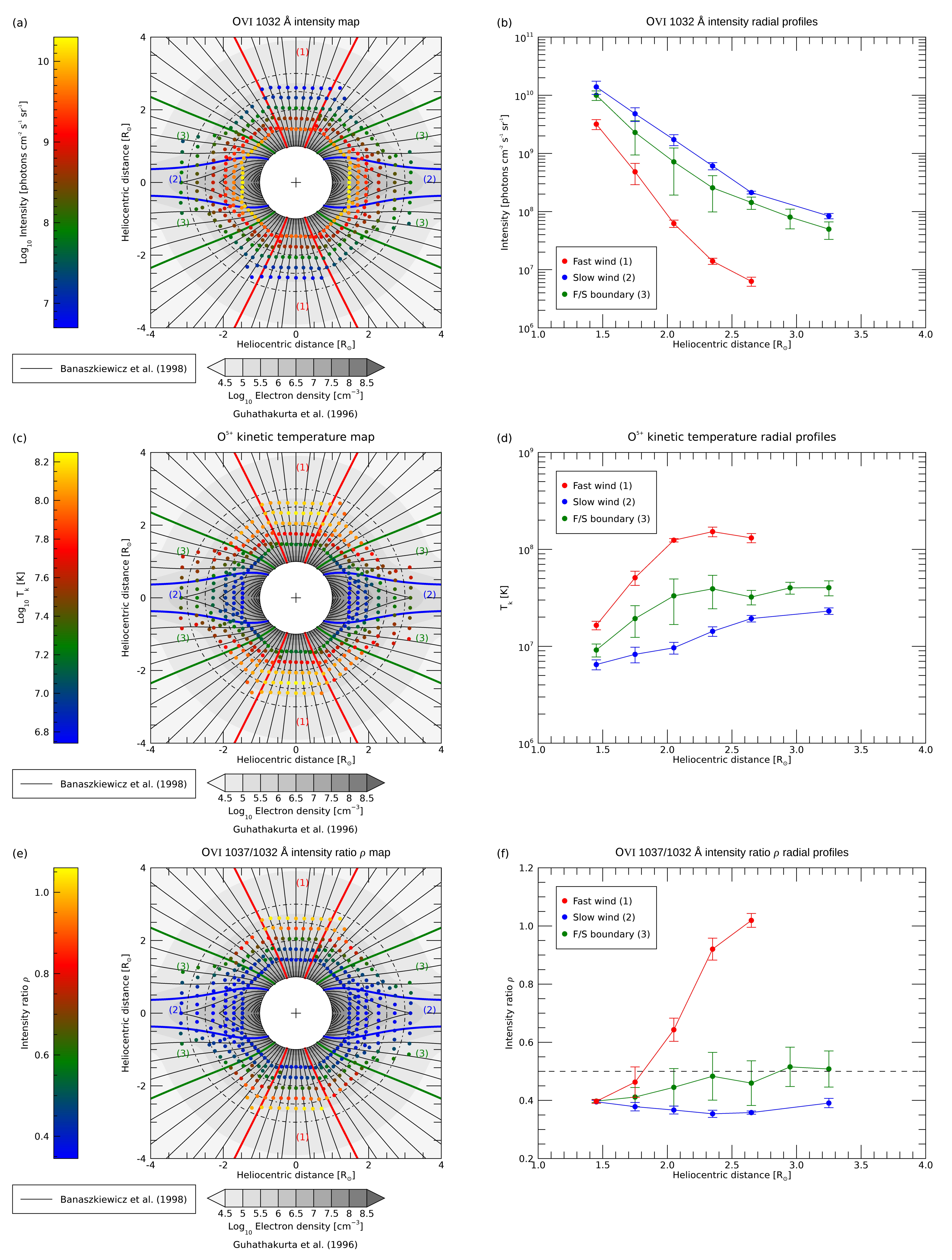
From top to bottom, the left panels of Figure 1 show 2D maps of the intensity of the O vi 1032 Å spectral line, kinetic temperature of the oxygen ions and O vi Å doublet intensity ratio . Each point in the maps represents the -wide portion of slit considered in the analysis and reports the corresponding value averaged over time from 5 May 1996 to 12 August 1997. Overlaid are the magnetic field lines by Banaszkiewicz et al. [53] and the electron isodensity contours by Guhathakurta et al. [54], representative of a dipolar solar minimum corona. UVCS results within the coronal regions referring to fast wind (i.e, polar coronal holes), slow wind (i.e., equatorial streamers) and fast/slow wind boundary (i.e., coronal hole edges adjacent to the streamers), as delimited in the maps by colored thicker magnetic field lines, are averaged in steps of R, in order to obtain radial profiles from to R. These are displayed (along with the corresponding standard deviation error bars) in the right panels of Figure 1. The magnetic field lines delimiting the fast, slow and boundary regions are rooted at 14, 50, and to the polar axis, respectively. Specifically, the lines defining the slow-wind regions (blue) are those closest to the equator not yet closed at the distances observed by UVCS; those delimiting the sources of high-speed streams (red) ensure instead to define a coronal hole core at most wide while encompassing (almost) all UVCS observations acquired at maximum height at PA = 0. Finally, the lines chosen to define the fast/slow wind boundary regions (green) are those that provide comparable statistics with respect to the slow and fast wind regions. It is worth noting that, to ensure statistical significance, the same analysis was also accomplished by considering slightly different delimiting field lines (while still fulfilling the above criteria). The results obtained fully confirmed those presented in the following.
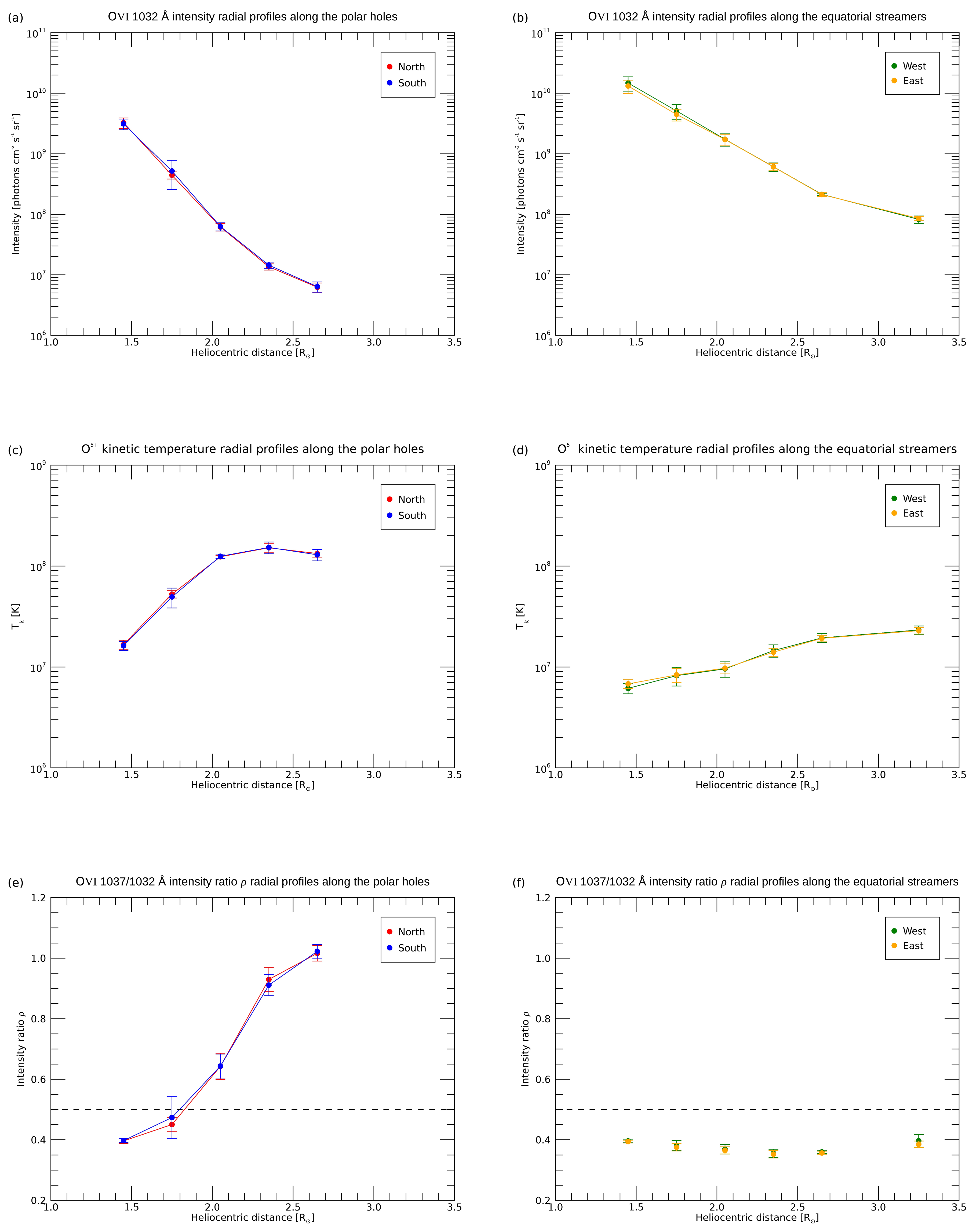
In order to ascertain any possible polar or axial coronal asymmetry, either in UV emission or in temperature/velocity, Figure 2 shows the radial profiles of each considered UVCS-based coronal parameter, along the coronal hole cores (left panels) and the equatorial streamers (right panels), but distinguishing between North (red) and South (blue) poles and between west (green) and east (orange) limbs.
3. Discussion of the Results
Looking at the results reported in the figures of the previous section as a whole, the first observational evidence that clearly emerges is the strikingly prominent dipolar structure of the solar minimum corona, characterized by large polar coronal holes and an equatorial streamer belt. This is the first time that such a topological configuration is statistically evidenced for the UV corona. As a matter of fact, the maps provided by Giordano et al. [46], Dolei et al. [47] and Dolei et al. [48] do not depict as clearly as in the present work the dipolar configuration of the UV corona (probably due to poor statistics and/or the use of the H i Ly as a wind diagnostic, as in [48], which, as discussed above, is not suited to this purpose). Not only is the dipolar geometry evident in the intensity of the O vi 1032 Å spectral line (Figure 1a), so is it also in the kinetic temperature (Figure 1c) and the expansion rate (Figure 1e) of the oxygen component of the solar wind. This seemingly straightforward result, which instead comes from analyzing hundreds of UVCS datasets over a two-year period, allows for the following picture to be drawn: at least at the solar minimum, the large-scale magnetic field topology is the main driver of the thermodynamic and hydrodynamic properties of the solar corona.
More specifically, the core of the polar coronal holes, where the plasma is heated at the highest temperatures in the entire corona (red radial profile in Figure 1d), represents the primary source of the fast solar wind (red dots in Figure 1f). There, the lowest divergence of the field lines ensures that the large amount of energy available is deposited beyond the sonic point (located at R, as statistically shown by [44]), thus, allowing the wind to be effectively accelerated as early as 5 R to values close to those observed in high-speed streams in the heliosphere [25]. Moving from the polar regions of the coronal holes toward their peripheral zones, the divergence of the field lines progressively increases and the coronal temperature decreases (green radial profile in Figure 1d). The combined effect of a sonic point located at higher heights [20], due to the more divergent field lines and less available energy, causes the solar wind acceleration process to be significantly less efficient. As a result, the outflow velocity of the expanding coronal plasma decreases with increasing divergence of the magnetic field lines when approaching the edges of the coronal hole (green dots in Figure 1f). The coupling between coronal temperature/outflow velocity and magnetic field divergence culminates along the boundary regions separating coronal holes from equatorial streamers, where the expansion factor of the field lines is no longer monotonic but first divergent and then convergent according to the streamer morphology. It is where the coronal temperatures are at least one order of magnitude lower than at the poles (blue curve in Figure 1d) and the plasma is accelerated to the slow solar wind regime (blue curve in Figure 1f).
This statistical result thereby establishes that during the the low activity phases of the solar cycle, the flanks of the streamers represent one of the coronal sources of the slow solar wind, thus strongly supporting the scenario drawn by Antonucci et al. [26], in which the low-speed plasma does indeed flow along the streamer boundaries. One, but not the only one, it is worth pointing out here: other sources may actually participate in the acceleration of the slow solar wind. Indeed, the values of the O vi doublet intensity ratio found in the core of streamers (, Figure 1f) are consistent with a very small-velocity coronal plasma (≲50 km s), though not static. It follows that according to the model proposed by Noci et al. [32], a component of the slow solar wind (the slowest, actually) may flow between the three-loop system constituting the complex structure of quiescent streamers. The two flux tubes delimited by the three so-formed current sheets and channeling the outflowing plasma first widen and then considerably shrink with height, causing “de facto” the wind to be slow.
Interestingly, on average, the dipolar solar minimum corona exhibits a striking symmetric configuration with respect to both the equator (i.e., North–South pole symmetry), and the rotation axis (i.e., west–east limb symmetry). This symmetry not only holds for the UV emission (top panels of Figure 2), but also and more remarkably for the kinetic temperature (middle panels) and expansion rate (bottom panels) of oxygen ions. This does not exclude the possibility that during the solar minimum period, there may be instants when the corona may be asymmetric, but should caution against making easy claims based on case studies (e.g., [48]). As a matter of fact, the results outlined in this work clearly indicate that the two poles of the solar minimum corona have the same magnetic field configuration, thus sharing similar areas and flux tube expansion factors, and are characterized by a comparable level of activity.
4. Concluding Remarks
This paper provides the first 2D maps of the UV solar corona that are statistically significant and therefore representative of the solar minimum of SC . The main benefit of statistical analyses over case studies is, in fact, the possibility of clearly ascertaining global average features of the solar corona that may otherwise remain at least partially unrevealed due to its intrinsic dynamical variability. Indeed, case studies’ results could be influenced by the particular corona conditions at the time of observation. It follows that only a statistical approach provides more reliable results, allowing for the establishment of large-scale coronal patterns, such as the radial evolution or latitudinal dependence of the most relevant solar wind plasma parameters, as well as the identification of the regions where the coronal heating and solar wind accelerations processes efficiently occur. (However, it is worth noting here that, on the other hand, only case studies can capture transient and local phenomena, which averaging procedures carried out over a long time period would inevitably blur. In this respect, case and statistical studies have their own (and mutual) benefit).
Specifically, this study clearly reports, for the first time in the literature, the dipolar structure of the corona, not only in its UV emission, but also evident by mapping the kinetic temperature and expansion rate of the solar wind oxygen component. In addition, it indicates which are, at solar minimum, the primary coronal sources of the slow solar wind, i.e., the flanks of the equatorial streamers and the flux tubes within the core of the streamers, and corroborates the ongoing paradigm that all of the fast wind is coming from polar coronal holes. Still in the spirit of showing how statistical studies can avoid drawing misleading conclusions, this work reveals that the corona is definitely axis-symmetric, in contrast to the claims raised by Dolei et al. [48] about a alleged North–South asymmetry in the coronal expansion rate, and based on a case study performed over a one-month interval in June 1997. It appears evident here that even if such asymmetry exists in June 1997, it is certainly not a global feature of the solar corona at the minimum of activity, but rather due to the temporal variability in coronal dynamics.
What is reported here is just a very first example of the outstanding scientific results that can be achieved from the analysis of UVCS survey data. A similar study performed at the minimum of activity of SC would allow for a comparison of the topological configurations of the solar corona during the two minima. Or, an analysis carried out at the solar maximum would shed light on the global characteristics of the corona during high activity phases, and reveal the sources of the slow solar wind, whether or not statistical asymmetries exist and what the average radial evolutions of temperature and outflow velocity are, depending on the latitude. Or, even, performing the same analysis but exploiting the H i Ly spectroscopic channel of UVCS, optimized for the investigation of the hydrogen component of the solar wind (the dominant one, actually), would allow scientists to deal with the still open problem concerning the possible difference between the expansion rates of the hydrogen atoms and oxygen ions, thus giving some clues about either the possible different mechanisms or the different efficiency of the same process underlying the heating and acceleration of the two components of the solar wind. Spectral analyses, accomplished at different heights from the Sun and at different latitudes, of crucial coronal parameters (i.e., UV emission, temperature and outflow velocity) are other interesting examples. It thus appears evident that although UVCS has stopped its instrumental activities in 2012, its data have a fundamental and crucial heritage, especially in terms of the key role they can play in support of coronal observations performed with the Metis coronagraph [55] aboard the Solar Orbiter [56], which, despite simultaneously imaging the solar corona in both white light and UV, does not have the capability of measuring its temperature. UVCS data will thus surely and significantly contribute to addressing the scientific goals of the Metis instrument and, more generally, the Solar Orbiter mission.
Funding
The author was partially supported by the Italian Space Agency (ASI) under contract 2018-30-HH.0.
Institutional Review Board Statement
Not applicable.
Informed Consent Statement
Not applicable.
Data Availability Statement
The raw UVCS data analyzed in this study are publicly available. They can be retrieved from the SOHO archive (https://sohowww.nascom.nasa.gov/data/archive/).
Acknowledgments
The author wishes to thank S. Giordano for his help in providing calibrated UVCS data.
Conflicts of Interest
The author declares no conflict of interest. The funders had no role in the design of the study; in the collection, analyses or interpretation of data; in the writing of the manuscript, or in the decision to publish the results.
References
- Aschwanden, M.J. Physics of the Solar Corona. An Introduction with Problems and Solutions, 2nd ed.; Springer: New York, NY, USA, 2005. [Google Scholar]
- Hundhausen, A.J. Coronal Expansion and Solar Wind; Springer: Berlin, Germany, 1972. [Google Scholar]
- See, V.; Jardine, M.; Vidotto, A.A.; Petit, P.; Marsden, S.C.; Jeffers, S.V.; do Nascimento, J.D. The effects of stellar winds on the magnetospheres and potential habitability of exoplanets. Astron. Astrophys. 2014, 570, A99. [Google Scholar] [CrossRef] [Green Version]
- Vidotto, A.A. Stellar Coronal and Wind Models: Impact on Exoplanets. In Handbook of Exoplanets; Deeg, H.J., Belmonte, J.A., Eds.; Springer: Cham, Switzerland, 2018; p. 26. [Google Scholar] [CrossRef] [Green Version]
- Linsky, J. Host Stars and their Effects on Exoplanet Atmospheres; Springer: Cham, Switzerland, 2019; Volume 955. [Google Scholar] [CrossRef]
- Wang, X.; Loeb, A. Nonthermal Emission from the Interaction of Magnetized Exoplanets with the Wind of Their Host Star. Astrophys. J. Lett. 2019, 874, L23. [Google Scholar] [CrossRef]
- Kay, C.; Airapetian, V.S.; Lüftinger, T.; Kochukhov, O. Frequency of Coronal Mass Ejection Impacts with Early Terrestrial Planets and Exoplanets around Active Solar-like Stars. Astrophys. J. Lett. 2019, 886, L37. [Google Scholar] [CrossRef]
- Telloni, D.; Carbone, F.; Antonucci, E.; Bruno, R.; Grimani, C.; Villante, U.; Giordano, S.; Mancuso, S.; Zangrilli, L. Study of the Influence of the Solar Wind Energy on the Geomagnetic Activity for Space Weather Science. Astrophys. J. 2020, 896, 149. [Google Scholar] [CrossRef]
- Telloni, D.; D’Amicis, R.; Bruno, R.; Perrone, D.; Sorriso-Valvo, L.; Raghav, A.N.; Choraghe, K. Alfvénicity-related Long Recovery Phases of Geomagnetic Storms: A Space Weather Perspective. Astrophys. J. 2021, 916, 64. [Google Scholar] [CrossRef]
- Viall, N.M.; Borovsky, J.E. Nine Outstanding Questions of Solar Wind Physics. J. Geophys. Res. Space Phys. 2020, 125, e26005. [Google Scholar] [CrossRef]
- Neugebauer, M.; Snyder, C.W. Solar Plasma Experiment. Science 1962, 138, 1095–1097. [Google Scholar] [CrossRef]
- Parker, E.N. Dynamics of the Interplanetary Gas and Magnetic Fields. Astrophys. J. 1958, 128, 664. [Google Scholar] [CrossRef]
- Domingo, V.; Fleck, B.; Poland, A.I. The SOHO Mission: An Overview. Sol. Phys. 1995, 162, 1–37. [Google Scholar] [CrossRef]
- Brueckner, G.E.; Howard, R.A.; Koomen, M.J.; Korendyke, C.M.; Michels, D.J.; Moses, J.D.; Socker, D.G.; Dere, K.P.; Lamy, P.L.; Llebaria, A.; et al. The Large Angle Spectroscopic Coronagraph (LASCO). Sol. Phys. 1995, 162, 357–402. [Google Scholar] [CrossRef]
- Kohl, J.L.; Esser, R.; Gardner, L.D.; Habbal, S.; Daigneau, P.S.; Dennis, E.F.; Nystrom, G.U.; Panasyuk, A.; Raymond, J.C.; Smith, P.L.; et al. The Ultraviolet Coronagraph Spectrometer for the Solar and Heliospheric Observatory. Sol. Phys. 1995, 162, 313–356. [Google Scholar] [CrossRef]
- Schwenn, R.; Inhester, B.; Plunkett, S.P.; Epple, A.; Podlipnik, B.; Bedford, D.K.; Eyles, C.J.; Simnett, G.M.; Tappin, S.J.; Bout, M.V.; et al. First View of the Extended Green-Line Emission Corona At Solar Activity Minimum Using the Lasco-C1 Coronagraph on SOHO. Sol. Phys. 1997, 175, 667–684. [Google Scholar] [CrossRef]
- Li, H.; Feng, X.; Wei, F. Is Solar Minimum 24/25 Another Unusual One? Astrophys. J. Lett. 2021, 917, L26. [Google Scholar] [CrossRef]
- Morgan, H.; Habbal, S.R. Observational Aspects of the Three-dimensional Coronal Structure Over a Solar Activity Cycle. Astrophys. J. 2010, 710, 1–15. [Google Scholar] [CrossRef]
- Koutchmy, S.; Livshits, M. Coronal Streamers. Space Sci. Rev. 1992, 61, 393–417. [Google Scholar] [CrossRef]
- Antonucci, E.; Harra, L.; Susino, R.; Telloni, D. Observations of the Solar Corona from Space. Space Sci. Rev. 2020, 216, 117. [Google Scholar] [CrossRef]
- Kohl, J.L.; Noci, G.; Antonucci, E.; Tondello, G.; Huber, M.C.E.; Cranmer, S.R.; Strachan, L.; Panasyuk, A.V.; Gardner, L.D.; Romoli, M.; et al. UVCS/SOHO Empirical Determinations of Anisotropic Velocity Distributions in the Solar Corona. Astrophys. J. Lett. 1998, 501, L127–L131. [Google Scholar] [CrossRef]
- Cranmer, S.R.; Kohl, J.L.; Noci, G.; Antonucci, E.; Tondello, G.; Huber, M.C.E.; Strachan, L.; Panasyuk, A.V.; Gardner, L.D.; Romoli, M.; et al. An Empirical Model of a Polar Coronal Hole at Solar Minimum. Astrophys. J. 1999, 511, 481–501. [Google Scholar] [CrossRef] [Green Version]
- Antonucci, E.; Dodero, M.A.; Giordano, S. Fast Solar Wind Velocity in a Polar Coronal Hole during Solar Minimum. Sol. Phys. 2000, 197, 115–134. [Google Scholar] [CrossRef]
- Leer, E.; Holzer, T.E. Energy addition in the solar wind. J. Geophys. Res. Space Phys. 1980, 85, 4681–4688. [Google Scholar] [CrossRef]
- Telloni, D.; Antonucci, E.; Dodero, M.A. Outflow velocity of the O+5 ions in polar coronal holes out to 5 R⊙. Astron. Astrophys. 2007, 472, 299–307. [Google Scholar] [CrossRef] [Green Version]
- Antonucci, E.; Abbo, L.; Dodero, M.A. Slow wind and magnetic topology in the solar minimum corona in 1996–1997. Astron. Astrophys. 2005, 435, 699–711. [Google Scholar] [CrossRef] [Green Version]
- Abbo, L.; Antonucci, E.; Mikić, Z.; Linker, J.A.; Riley, P.; Lionello, R. Characterization of the slow wind in the outer corona. Adv. Space Res. 2010, 46, 1400–1408. [Google Scholar] [CrossRef] [Green Version]
- Wang, Y.M. Two Types of Slow Solar Wind. Astrophys. J. Lett. 1994, 437, L67. [Google Scholar] [CrossRef]
- Antonucci, E. Wind in the Solar Corona: Dynamics and Composition. Space Sci. Rev. 2006, 124, 35–50. [Google Scholar] [CrossRef]
- Antonucci, E.; Abbo, L.; Telloni, D. UVCS Observations of Temperature and Velocity Profiles in Coronal Holes. Space Sci. Rev. 2012, 172, 5–22. [Google Scholar] [CrossRef]
- Nerney, S.; Suess, S.T. Stagnation Flow in Thin Streamer Boundaries. Astrophys. J. 2005, 624, 378–391. [Google Scholar] [CrossRef]
- Noci, G.; Kohl, J.L.; Antonucci, E.; Tondello, G.; Huber, M.C.E.; Fineschi, S.; Gardner, L.D.; Korendyke, C.M.; Nicolosi, P.; Romoli, M.; et al. The quiescent corona and slow solar wind. In Proceedings of the Fifth SOHO Workshop: The Corona and Solar Wind Near Minimum Activity, Kiruna, Sweden, 17–20 June 1997; Wilson, A., Ed.; ESA Special Publication: The Hague, The Netherlands, 1997; Volume 404, p. 75. [Google Scholar]
- Smith, E.J.; Tsurutani, B.T.; Rosenberg, R.L. Observations of the interplanetary sector structure up to heliographic latitudes of 16°: Pioneer 11. J. Geophys. Res. Space Phys. 1978, 83, 717–724. [Google Scholar] [CrossRef]
- D’Amicis, R.; Matteini, L.; Bruno, R. On the slow solar wind with high Alfvénicity: From composition and microphysics to spectral properties. Mon. Not. R. Astron. Soc. 2019, 483, 4665–4677. [Google Scholar] [CrossRef]
- Wenzel, K.P.; Marsden, R.G.; Page, D.E.; Smith, E.J. The ULYSSES Mission. Astron. Astrophys. Suppl. Ser. 1992, 92, 207. [Google Scholar]
- McComas, D.J.; Barraclough, B.L.; Funsten, H.O.; Gosling, J.T.; Santiago-Muñoz, E.; Skoug, R.M.; Goldstein, B.E.; Neugebauer, M.; Riley, P.; Balogh, A. Solar wind observations over Ulysses’ first full polar orbit. J. Geophys. Res. Space Phys. 2000, 105, 10419–10434. [Google Scholar] [CrossRef]
- McComas, D.J.; Elliott, H.A.; Schwadron, N.A.; Gosling, J.T.; Skoug, R.M.; Goldstein, B.E. The three-dimensional solar wind around solar maximum. Geophys. Res. Lett. 2003, 30, 1517. [Google Scholar] [CrossRef]
- Antonucci, E. Solar Wind Acceleration Region. In Proceedings of the 8th SOHO Workshop: Plasma Dynamics and Diagnostics in the Solar Transition Region and Corona, Paris, France, 22–25 June 1999; Vial, J.C., Kaldeich-Schü, B., Eds.; ESA Special Publication: The Hague, The Netherlands, 1999; Volume 446, p. 53. [Google Scholar]
- Cranmer, S.R. Ion Cyclotron Wave Dissipation in the Solar Corona: The Summed Effect of More than 2000 Ion Species. Astrophys. J. 2000, 532, 1197–1208. [Google Scholar] [CrossRef] [Green Version]
- Kohl, J.L.; Noci, G.; Cranmer, S.R.; Raymond, J.C. Ultraviolet spectroscopy of the extended solar corona. Astron. Astrophys. Rev. 2006, 13, 31–157. [Google Scholar] [CrossRef]
- Cranmer, S.R.; van Ballegooijen, A.A. Can the Solar Wind be Driven by Magnetic Reconnection in the Sun’s Magnetic Carpet? Astrophys. J. 2010, 720, 824–847. [Google Scholar] [CrossRef] [Green Version]
- Zank, G.P.; Zhao, L.L.; Adhikari, L.; Telloni, D.; Kasper, J.C.; Bale, S.D. Turbulence transport in the solar corona: Theory, modeling, and Parker Solar Probe. Phys. Plasmas 2021, 28, 080501. [Google Scholar] [CrossRef]
- Telloni, D.; Antonucci, E.; Dodero, M.A. Oxygen temperature anisotropy and solar wind heating above coronal holes out to 5 R⊙. Astron. Astrophys. 2007, 476, 1341–1346. [Google Scholar] [CrossRef] [Green Version]
- Telloni, D.; Giordano, S.; Antonucci, E. On the Fast Solar Wind Heating and Acceleration Processes: A Statistical Study Based on the UVCS Survey Data. Astrophys. J. Lett. 2019, 881, L36. [Google Scholar] [CrossRef]
- Strachan, L.; Panasyuk, A.V.; Kohl, J.L.; Lamy, P. The Evolution of Plasma Parameters on a Coronal Source Surface at 2.3 R⊙ during Solar Minimum. Astrophys. J. 2012, 745, 51. [Google Scholar] [CrossRef] [Green Version]
- Giordano, S.; Antonucci, E.; Benna, C.; Kohl, J.L.; Noci, G.; Michels, J.; Fineschi, S. Solar Wind Acceleration in the Solar Corona. In Correlated Phenomena at the Sun, in the Heliosphere and in Geospace; Wilson, A., Ed.; ESA Special Publication: The Hague, The Netherlands, 1997; Volume 415, p. 327. [Google Scholar]
- Dolei, S.; Spadaro, D.; Ventura, R. Mapping the coronal hydrogen temperature in view of the forthcoming coronagraph observations by Solar Orbiter. Astron. Astrophys. 2016, 592, A137. [Google Scholar] [CrossRef]
- Dolei, S.; Susino, R.; Sasso, C.; Bemporad, A.; Andretta, V.; Spadaro, D.; Ventura, R.; Antonucci, E.; Abbo, L.; Da Deppo, V.; et al. Mapping the solar wind HI outflow velocity in the inner heliosphere by coronagraphic ultraviolet and visible-light observations. Astron. Astrophys. 2018, 612, A84. [Google Scholar] [CrossRef] [Green Version]
- Withbroe, G.L.; Kohl, J.L.; Weiser, H.; Munro, R.H. Probing the solar wind acceleration region using spectroscopic techniques. Space Sci. Rev. 1982, 33, 17–52. [Google Scholar] [CrossRef]
- Dodero, M.A.; Antonucci, E.; Giordano, S.; Martin, R. Solar Wind Velocity and Anisotropic Coronal Kinetic Temperature Measured with the O vi Doublet Ratio. Sol. Phys. 1998, 183, 77–90. [Google Scholar] [CrossRef]
- Noci, G.; Kohl, J.L.; Withbroe, G.L. Solar Wind Diagnostics from Doppler-enhanced Scattering. Astrophys. J. 1987, 315, 706. [Google Scholar] [CrossRef]
- Noci, G.; Gavryuseva, E. Plasma Outflows in Coronal Streamers. Astrophys. J. Lett. 2007, 658, L63–L66. [Google Scholar] [CrossRef]
- Banaszkiewicz, M.; Axford, W.I.; McKenzie, J.F. An analytic solar magnetic field model. Astron. Astrophys. 1998, 337, 940–944. [Google Scholar]
- Guhathakurta, M.; Holzer, T.E.; MacQueen, R.M. The Large-Scale Density Structure of the Solar Corona and the Heliospheric Current Sheet. Astrophys. J. 1996, 458, 817. [Google Scholar] [CrossRef]
- Antonucci, E.; Romoli, M.; Andretta, V.; Fineschi, S.; Heinzel, P.; Moses, J.D.; Naletto, G.; Nicolini, G.; Spadaro, D.; Teriaca, L.; et al. Metis: The Solar Orbiter visible light and ultraviolet coronal imager. Astron. Astrophys. 2020, 642, A10. [Google Scholar] [CrossRef]
- Müller, D.; St. Cyr, O.C.; Zouganelis, I.; Gilbert, H.R.; Marsden, R.; Nieves-Chinchilla, T.; Antonucci, E.; Auchère, F.; Berghmans, D.; Horbury, T.S.; et al. The Solar Orbiter mission. Science overview. Astron. Astrophys. 2020, 642, A1. [Google Scholar] [CrossRef]
Figure 1.
2D maps of the O vi 1032 Å line intensity (a), O kinetic temperature (c) and O vi Å doublet intensity ratio (e) measured with UVCS in the solar corona. Superimposed are typical solar minimum models for the magnetic field dipole configuration [53] and (in tonalities of grey) for the electron density distribution [54]. Dash-dotted circles at , , and R are drawn for reference. The corresponding radial profiles are shown in (b,d,f), respectively. Red, blue and green curves refer to the coronal regions bound in the maps by thicker same-colored magnetic field lines and corresponding to the fast wind (1), slow wind (2) and fast/slow wind boundary regions (3), respectively. Standard deviation uncertainties are displayed as error bars. , roughly corresponding to an outflow velocity of 100 km s [51], is marked as a horizontal dashed line in (f).

Figure 2.
Radial profiles of the O vi 1032 Å line intensity along coronal hole cores (a) and equatorial streamers (b). Analogous polar/equatorial radial profiles but for the O kinetic temperature and O vi Å doublet intensity ratio are shown in (c–f), respectively. Red, blue, green and orange colors refer to North and South poles, and to west and east limbs, respectively. Standard deviation error bars are also displayed. The horizontal dashed line in (e,f) indicates an expansion rate of about 100 km s.

Publisher’s Note: MDPI stays neutral with regard to jurisdictional claims in published maps and institutional affiliations. |
© 2021 by the author. Licensee MDPI, Basel, Switzerland. This article is an open access article distributed under the terms and conditions of the Creative Commons Attribution (CC BY) license (https://creativecommons.org/licenses/by/4.0/).
Share and Cite
MDPI and ACS Style
Telloni, D. The Dipolar Solar Minimum Corona. Universe 2021, 7, 507. https://0-doi-org.brum.beds.ac.uk/10.3390/universe7120507
AMA Style
Telloni D. The Dipolar Solar Minimum Corona. Universe. 2021; 7(12):507. https://0-doi-org.brum.beds.ac.uk/10.3390/universe7120507
Chicago/Turabian StyleTelloni, Daniele. 2021. "The Dipolar Solar Minimum Corona" Universe 7, no. 12: 507. https://0-doi-org.brum.beds.ac.uk/10.3390/universe7120507
Note that from the first issue of 2016, this journal uses article numbers instead of page numbers. See further details here.