
De Sitter Solutions in Einstein–Gauss–Bonnet Gravity †


Skobeltsyn Institute of Nuclear Physics, Lomonosov Moscow State University, Leninskie Gory 1, 119991 Moscow, Russia
*
Author to whom correspondence should be addressed.
†
This paper is an extended version from the proceeding paper: Sergey Vernov and Ekaterina Pozdeeva. De Sitter Solutions in Models with the Gauss-Bonnet Term. In Proceedings of the 1st Electronic Conference on Universe, online, 22–28 February 2021.
Universe 2021, 7(5), 149; https://0-doi-org.brum.beds.ac.uk/10.3390/universe7050149
Submission received: 23 April 2021
/
Revised: 12 May 2021
/
Accepted: 12 May 2021
/
Published: 16 May 2021
(This article belongs to the Special Issue Selected Papers from the 1st International Electronic Conference on Universe (ECU 2021))
Abstract
:De Sitter solutions play an important role in cosmology because the knowledge of unstable de Sitter solutions can be useful to describe inflation, whereas stable de Sitter solutions are often used in models of late-time acceleration of the Universe. The Einstein–Gauss–Bonnet gravity cosmological models are actively used both as inflationary models and as dark energy models. To modify the Einstein equations one can add a nonlinear function of the Gauss–Bonnet term or a function of the scalar field multiplied on the Gauss–Bonnet term. The effective potential method essentially simplifies the search and stability analysis of de Sitter solutions, because the stable de Sitter solutions correspond to minima of the effective potential.
1. Introduction
Cosmological models with scalar fields play a central role in the description of the global evolution of the Universe. In particular, modified gravity models with the Ricci scalar multiplied by a function of the scalar field are very popular [1,2,3,4]. These models are quite natural because quantum corrections to the effective action with a minimally coupled scalar field include nonminimal coupling terms [5,6,7]. Many inflationary models that connect cosmology and particle physics include nonminimally coupled scalar fields [8,9,10,11,12,13,14,15,16,17,18,19,20,21,22,23,24].
It is well-known that one can add the Gauss–Bonnet term to the Hilbert–Einstein Lagrangian of the General Relativity and it does not change the equations of motion. On the other hand, this term multiplied by some nonconstant function of a scalar field modifies the equations of motion. Models with both the Ricci scalar and the Gauss–Bonnet term multiplied by some functions of the scalar field are natural generalizations of the models with a minimal coupling [25,26,27]. Furthermore, models with a nonlinear function of the Gauss–Bonnet term can be rewritten in the equivalent form that includes a scalar field without kinetic term [28,29,30,31].
The cosmological models with the Gauss–Bonnet term are motivated by the string theory [30,31,32,33,34,35,36,37] and are actively used for describing of both the early Universe evolution (inflation) [25,26,27,38,39,40,41,42,43,44,45,46,47,48,49,50,51,52,53,54,55,56,57] and the current dark energy dominated epoch [28,29,30,31,36,37,58,59,60,61,62,63,64,65,66]. Note that both stages of the Universe evolution are characterized by the quasi de Sitter accelerated expansion of the Universe. So, it is important to have an effective method for the searching of de Sitter solutions and the study of their stability. The method proposed in [67] solves this problem for the Gauss–Bonnet model with the standard scalar field. It is a generalization of the effective potential method for models with scalar field nonminimally coupled to the curvature only [68,69,70]. We have shown in Ref. [27] that the effective potential is a useful tool to generalize the known inflationary models with the Gauss–Bonnet term. On the one hand, the effective potential allows to rule out models with a stable de Sitter solution, for which it is difficult to construct an inflationary scenario with a graceful exit. Models with unstable de Sitter solutions or without an exact de Sitter solution are more suitable. On the other hand, the scalar spectral index and the amplitude of the scalar perturbations as functions of the e-folding number can be expressed via derivatives of the effective potential [27,55,57].
In this paper, we generalize the effective potential method on models with nonlinear functions of the Gauss–Bonnet term that can be presented as models with a scalar field without kinetic term. We also show that the situation is more difficult in the case of a phantom scalar field.
The paper is organized as follows. In Section 2, we remind the evolution equations of the model considered and the standard way for the search of de Sitter solutions. In Section 3, we analyze the stability of de Sitter solutions due to the effective potential. A way of constructing different models with the same structure of de Sitter solutions is proposed in Section 4. In Section 5, we analyze the stability of de Sitter solutions in the proposed type of gravity models. Section 6 is devoted to our conclusions.
2. Models the Gauss–Bonnet Term
Let us consider the model with the Gauss–Bonnet term described by the following action:
where the functions , , and are double differentiable ones, c is a constant, R is the Ricci scalar and is the Gauss–Bonnet term,
As known [29,31], the action
where is a constant and is a double differentiable function, can be rewritten in the form of action (1) with :
where a prime denotes the derivatives with respect to . Varying action (3) over , one gets and the initial model.
In the spatially flat Friedmann–Lemaître–Robertson–Walker metric with the interval
where is the scale factor, one gets the following evolution equations [56]:
where is the Hubble parameter, dots and primes denote the derivatives with respect to the cosmic time and the scalar field , respectively. At , these equations have been investigated in many papers (see, for example [25,56,67]).
To find de Sitter solutions with a constant in the model (2) we substitute and into Equations (5) and (7). A de Sitter solution does not depend on the value of c, so we obtain the same results as in the case of considered in [67]:
and
where for any function A. Therefore, for arbitrary functions and with , we can choose such that the corresponding point becomes a de Sitter solution, with the Hubble parameter defined by Equation (8). We always choose that .
3. Stability of de Sitter Solutions
To analyze the stability of a de Sitter solution we transform Equations (6) and (7) to the following dynamical system:
where
In the case , the last equation is essentially simplified:
At a de Sitter point system (10) is
that corresponds to .
In Ref. [67], the effective potential has been proposed for models with the Gauss–Bonnet term:
Using Equations (8) and (12), we obtain
therefore, de Sitter solutions correspond to extremum points of the effective potential .
To investigate the Lyapunov stability of a de Sitter solution we use the following expansions:
where is a small parameter. Therefore,
where
The functions , , and are connected by Equation (5):
This expression does not depend on the value of c and coincides with the corresponding expression obtained in Ref. [67].
Substituting (16)–(18) into Equation (10) in the first order of , we obtain the following system of two linear differential equations:
where
This system can be rewritten in the matrix form:
where the matrix
The general solution of system (22) has the following form:
where are some constants. Solving the characteristic equation:
we get the following roots:
A de Sitter solution is stable if real parts of both and are negative. We consider the case
hence, .
In the case of a positive , we see that for and the condition is equivalent to . In the cases and , a de Sitter solution is stable if and unstable if .
In the case of , we see that can be negative. So, in this case de Sitter solution is stable if the . So, the main result of Ref. [67] can be generalized on the case without any correction, whereas the condition should be change to in the case of that corresponds to a phantom scalar field .
4. Different Models with the Same Structure of de Sitter Solutions
It is evident that any change of functions U and V can be compensated by the change of function F such that the first derivative of the effective potential does not change. This property can be used for the generalization of the inflationary scenarios [27]. Let us consider a more nontrivial question: how one can change the functions U and V only to obtain the model with the same structure of de Sitter solutions. To be concrete we seek for models with the same values of and the same stability properties of de Sitter solutions, but maybe with different values of .
Considering the stability analysis of de Sitter solutions, we define the effective potential as such a function that its minima correspond to the stable de Sitter solutions and maxima correspond to unstable de Sitter solutions. For this reason, the effective potential is not unique. We can add a constant to it or multiply it on a positive number. If we transform functions and to functions and
then the effective potentials of the original and transformed models are connected as follows:
Therefore, the structure of de Sitter solutions does not change if the function , where a constant and is an arbitrary constant. Furthermore, one should check that and for all de Sitter solutions.
Moreover, if for any , then the functions and , where n is a natural number, can be considered as new effective potentials. Different transformations of the effective potential can be combined, for example, functions and can be considered as effective potentials if for any . So, transformations of the model with or does not change the structure of de Sitter solutions.
5. Examples of Models
5.1. Evolution Equations
Several examples of models with an ordinary scalar field coupled with the Gauss–Bonnet term have been considered in Refs. [55,67]. In this paper, we consider examples in the case of , namely, the case of model, described by the following action:
where is a double differentiable function, , , and are constants. A linear function corresponds to the General Relativity, whereas a nonlinear function corresponds to the modified gravity. Note that and models are particular cases of the model considered.
In the case of a nonlinear function , action (29) can be rewritten in the following form:
Varying action (30) over , one gets and the initial model with action (29). Action (30) is a particular case of action (1) with the functions:
The effective potential is the following combination of the function and its first derivative:
So,
and a point with correspond to de Sitter solutions if and . Furthermore, the second multiplied can be equal to zero that also can correspond to a de Sitter solution. We explorer de Sitter solutions in detail in a few examples of models.
5.2. The Function F in a Role of the Effective Potential
If , where C is a constant, then and the function plays the role of the effective potential. For the considering models the condition is the following first order differential equation
This equation has two solutions:
where A is an integration constant. The function is a linear one, so this case is the General Relativity model with the cosmological constant. In the case of the function , the function F is a linear one and this model has no de Sitter solution.
5.3. The Case of a Power Function of the Gauss–Bonnet Term
There is no de Sitter solutions at . So, we consider only such values of that is real and negative at and obtain
Let us consider several examples:
- 1.
- At , we get de Sitter solution
The effective potential
and its second derivative is negative: . Therefore, we can conclude that the de Sitter solution is unique and unstable.
- 2.
- At we get
The potential
The condition demands for . Using
we get that the considered model with and has an unstable de Sitter solution.
- 3.
So, a de Sitter solution exist if and only if and it is unstable.
5.4. The Case of a Quadratic Polynomial
5.4.1. Equation for
Let us consider the case of
where are constants, . In this case,
where . Note that the function F is defined up to a constant, so we can put without loss of generality.
De Sitter solution corresponds to that is a solution of the following equation:
Let us consider a few interesting particular cases of this equation.
5.4.2. The Case Gravity
If , then the model has no Gauss–Bonnet term and is a gravity model with the effective potential
Equation (46) is a quadratic one and has the following two solutions:
The point does not correspond to de Sitter solution because of . At , we get
At de Sitter point , we obtain
From Equation (8), we get
a de Sitter solution exists only if . Note that the Starobinsky inflationary model [71,72,73] does not include the cosmological constant, so, . In this case, a de Sitter solution does not exist. The potential for all values of if and . In this case, the de Sitter solution is stable.
5.4.3. The Case Gravity
If , then the model is a gravity models with the effective potential
The value of at a de Sitter point is a real solution of the following equation:
In the case of , one gets the following real solutions of Equation (53):
Note that does not correspond to a de Sitter solution, because . So, we get the unique de Sitter solution .
At the de Sitter point, the second derivative of the effective potential is
Furthermore, we demand that , so, and we get a model with one unstable de Sitter solution.
5.4.4. The Case of the Absence of the Cosmological Constant
In the case of , the potential , therefore, and are necessary condition for de Sitter solution existence. Assuming that , we obtain the first derivative of the effective potential in the following form:
where
The effective potential can be multiplied on any positive constant, so we can consider the function
instead of and the number of its zeros depends on values of parameters and only.
The function
is not always positive, so it is possible that an extremum of the effective potential does not corresponds to de Sitter solution. The sign of depends on the sign of the parameter , whereas does not depend on the sign of the parameter . Note that the functions U and J are not equal to zero at the same point, because .
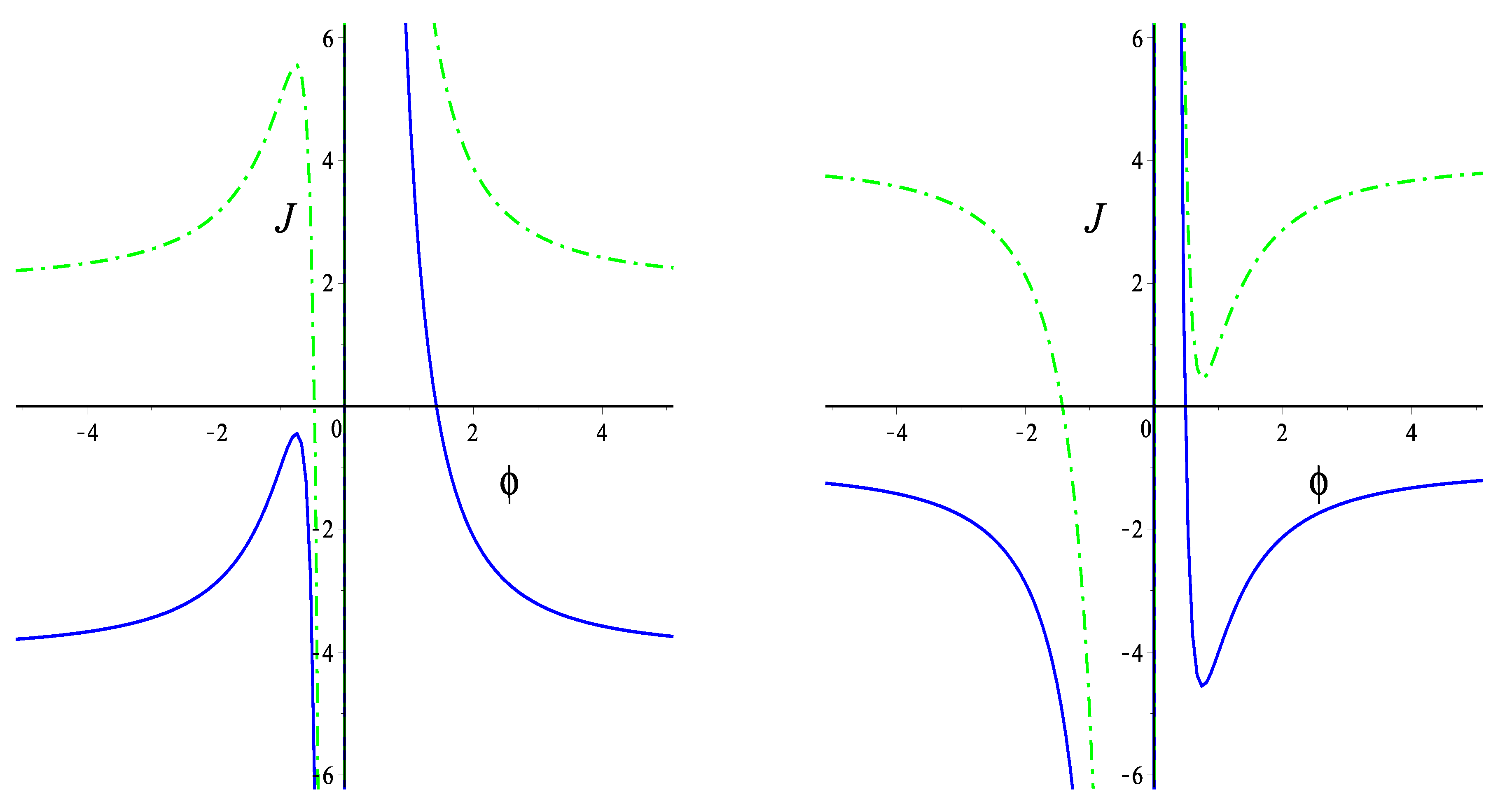
The same values of parameters and correspond both to models with one de Sitter solution and to models without de Sitter solution in dependence of the sign of . A decreasing behavior of the function J in the neighborhood of corresponds to an unstable de Sitter solution. In Figure 1, blue solid curves and green dash-dot curves correspond to models either with one unstable de Sitter solution or without de Sitter solutions in dependence of the sign of .
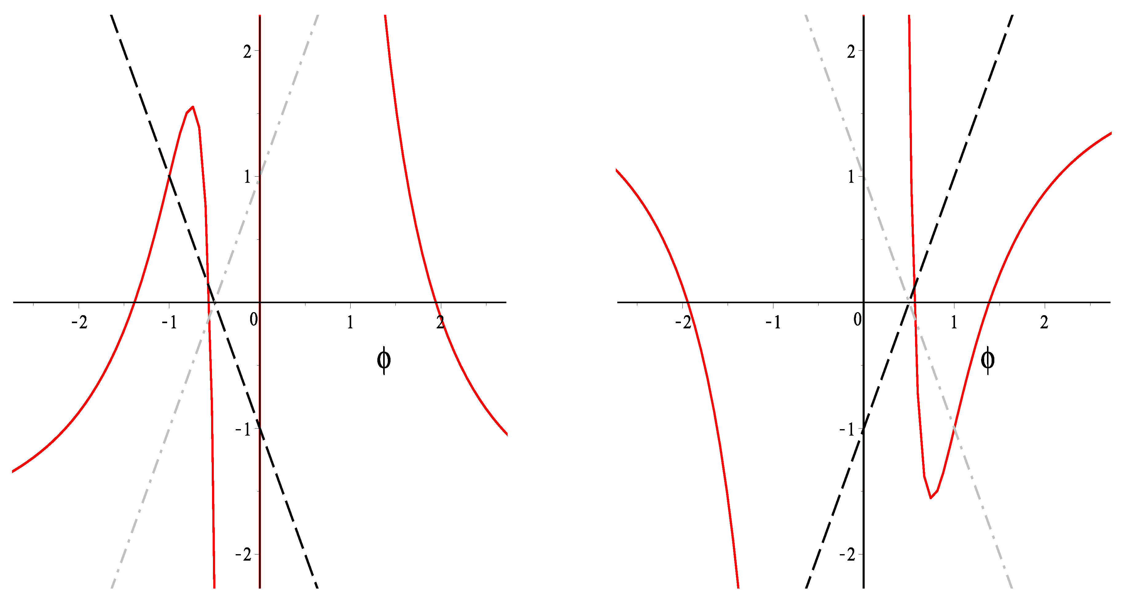
In Figure 2, we present the function that has three roots (red solid curves) and the function for the same values of parameters and and the parameter . One can see that the model has one unstable de Sitter solution or one stable and one unstable de Sitter solutions in dependence on the sign of . The crosses of gray and black lines with axis correspond to switch of gravity and antigravity regimes in the model considered.
6. Conclusions
In this paper, we consider de Sitter solutions in models with the Gauss–Bonnet term, including gravity models. We investigate evolution equations of a scalar field nonminimally coupled both with the curvature and with the Gauss–Bonnet term and look for the fixed points of scalar field dynamics which correspond to de Sitter solutions. We show that, in the case of a positive coupling function , it is possible to introduce an effective potential which can be expressed through the function U of nonminimal coupling with the curvature, the scalar field potential V, and the coupling function with the Gauss–Bonnet term denoted by F. We show that it is convenient to investigate the structure of fixed points using the effective potential because the stable de Sitter solutions correspond to minima of the effective potential. The existence and stability of de Sitter solutions in the system under consideration can be studied with the help of function since one can get the structure and stability properties of de Sitter solutions using a graphical representation of the effective potential only. It should be noted that the effective potential is not uniquely defined. We can multiply it on a positive constant or add a constant to it. If the effective potential is a positive definite function, then we can consider and , where n is a natural number, like other forms of the effective potential.
In this paper, we show that the effective potential proposed [67] for models with the Gauss–Bonnet term multiplied on a function of the scalar field can be used in models as well. To find de Sitter solutions in some model, we rewrite the action of this model in the form (30) and construct the corresponding effective potential . A stable de Sitter solutions corresponds , where the values of the scalar field at de Sitter point is determined by the condition . We have found de Sitter solutions in a few models to demonstrate the effective potential method.
Note that the proposed effective potential is a useful tool for the construction of inflationary scenarios in the models with the Gauss–Bonnet term multiplied to a function of the scalar field [27,55,57]. It is interesting that in the slow-roll approximation the scalar spectral index and the amplitude of the scalar perturbations as functions of the e-folding number can be expressed via derivatives of the effective potential given in the form (14). Furthermore, the knowledge of unstable de Sitter solutions can be useful to describe inflation (see, for example, Ref. [20]). We plan to generalize this approach to inflationary scenarios in models.
The search for stable de Sitter solutions is important for models that explain the late-time accelerated expansion of the Universe [29,59,60,62,65,66]. A generic action can be transformed into one linear in R and by including of two scalar fields, whereas the proposed special type of such models describing by action (29) can be linearized in R and by including of one scalar field without kinetic term. It allows to use the effective potential method and to simplify analysis of the stability of de Sitter solutions in distinguish to the traditional approach [62]. The proposed models include not only and gravity models, but also more complicated models with the function in the action. We plan to investigate a possibility to describe the late-time accelerated expansion of the Universe in such types of models taking into account the observation restrictions.
Author Contributions
The authors contributed equally to this work. Investigation, S.V. and E.P.; Writing original draft, S.V. and E.P. All authors have read and agreed to the published version of the manuscript.
Funding
This work is partially supported by the Russian Foundation for Basic Research grant No. 20-02-00411.
Conflicts of Interest
The authors declare no conflict of interest.
References
- Capozziello, S.; Faraoni, V. Beyond Einstein Gravity: A Survey of Gravitational Theories for Cosmology and Astrophysics; Springer: New York, NY, USA, 2011. [Google Scholar]
- Capozziello, S.; De Laurentis, M. Extended Theories of Gravity. Phys. Rep. 2011, 509, 167–321. [Google Scholar] [CrossRef] [Green Version]
- Fujii, Y.; Maeda, K. The Scalar—Tensor Theory of Gravitation; Cambridge University Press: Cambridge, UK, 2004. [Google Scholar]
- Faraoni, V. Cosmology in Scalar—Tensor Gravity; Kluwer Academic: Dordrecht, The Netherlands, 2004. [Google Scholar]
- Chernikov, E.A.; Tagirov, E.A. Quantum theory of scalar fields in de Sitter space-time. Ann. Poincare Phys. Theor. A 1968, 9, 109. [Google Scholar]
- Tagirov, E.A. Consequences of field quantization in de Sitter type cosmological models. Ann. Phys. 1973, 76, 561. [Google Scholar] [CrossRef]
- Callan, C.G.; Coleman, S.R.; Jackiw, R. A New improved energy—Momentum tensor. Ann. Phys. 1970, 59, 42. [Google Scholar] [CrossRef]
- Barvinsky, A.O.; Kamenshchik, A.Y. Quantum scale of inflation and particle physics of the early universe. Phys. Lett. B 1994, 332, 270. [Google Scholar] [CrossRef] [Green Version]
- Bezrukov, F.L.; Shaposhnikov, M. The Standard Model Higgs boson as the inflaton. Phys. Lett. B 2008, 659, 703. [Google Scholar] [CrossRef] [Green Version]
- Barvinsky, A.O.; Kamenshchik, A.Y.; Starobinsky, A.A. Inflation scenario via the Standard Model Higgs boson and LHC. J. Cosmol. Asropart. Phys. 2008, 2008, 021. [Google Scholar] [CrossRef]
- De Simone, A.; Hertzberg, M.P.; Wilczek, F. Running Inflation in the Standard Model. Phys. Lett. B 2009, 678, 1. [Google Scholar] [CrossRef] [Green Version]
- Barvinsky, A.O.; Kamenshchik, A.Y.; Kiefer, C.; Starobinsky, A.A.; Steinwachs, C.F. Higgs boson, renormalization group, and cosmology. Eur. Phys. J. C 2012, 72, 2219. [Google Scholar] [CrossRef]
- Lerner, R.N.; McDonald, J. Higgs Inflation and Naturalness. J. Cosmol. Astropart. Phys. 2010, 1004, 015. [Google Scholar] [CrossRef] [Green Version]
- Bezrukov, F.L.; Magnin, A.; Shaposhnikov, M.; Sibiryakov, S. Higgs inflation: Consistency and generalisations. J. High Energy Phys. 2011, 1101, 016. [Google Scholar] [CrossRef] [Green Version]
- Greenwood, R.N.; Kaiser, D.I.; Sfakianakis, E.I. Multifield Dynamics of Higgs Inflation. Phys. Rev. D 2013, 87, 064021. [Google Scholar] [CrossRef] [Green Version]
- Bezrukov, F.L. The Higgs field as an inflaton. Class. Quant. Grav. 2013, 30, 214001. [Google Scholar] [CrossRef]
- Cerioni, A.; Finelli, F.; Tronconi, A.; Venturi, G. Inflation and Reheating in Induced Gravity. Phys. Lett. B 2009, 681, 383. [Google Scholar] [CrossRef] [Green Version]
- Kallosh, R.; Linde, A.; Roest, D. The double attractor behavior of induced inflation. J. High Energy Phys. 2014, 1409, 062. [Google Scholar] [CrossRef] [Green Version]
- Rinaldi, M.; Vanzo, L.; Zerbini, S.; Venturi, G. Inflationary quasi-scale invariant attractors. Phys. Rev. D 2016, 93, 024040. [Google Scholar] [CrossRef] [Green Version]
- Elizalde, E.; Odintsov, S.D.; Pozdeeva, E.O.; Vernov, S.Y. Renormalization-group inflationary scalar electrodynamics and SU(5) scenarios confronted with Planck2013 and BICEP2 results. Phys. Rev. D 2014, 90, 084001. [Google Scholar] [CrossRef] [Green Version]
- Elizalde, E.; Odintsov, S.D.; Pozdeeva, E.O.; Vernov, S.Y. Cosmological attractor inflation from the RG-improved Higgs sector of finite gauge theory. J. Cosmol. Astropart. Phys. 2016, 1602, 025. [Google Scholar] [CrossRef] [Green Version]
- Pozdeeva, E.O.; Vernov, S.Y. Renormalization-group improved inflationary scenarios. Phys. Part. Nucl. Lett. 2017, 14, 386. [Google Scholar] [CrossRef] [Green Version]
- Dubinin, M.N.; Petrova, E.Y.; Pozdeeva, E.O.; Sumin, M.V.; Vernov, S.Y. MSSM-inspired multifield inflation. J. High Energy Phys. 2017, 1712, 036. [Google Scholar] [CrossRef] [Green Version]
- Kamenshchik, A.Y.; Tronconi, A.; Venturi, G. Quantum cosmology and the inflationary spectra from a nonminimally coupled inflaton. Phys. Rev. D 2020, 101, 023534. [Google Scholar] [CrossRef] [Green Version]
- van de Bruck, C.; Longden, C. Higgs Inflation with a Gauss–Bonnet term in the Jordan Frame. Phys. Rev. D 2016, 93, 063519. [Google Scholar] [CrossRef] [Green Version]
- Mathew, J.; Shankaranarayanan, S. Low scale Higgs inflation with Gauss–Bonnet coupling. Astropart. Phys. 2016, 84, 1. [Google Scholar] [CrossRef] [Green Version]
- Pozdeeva, E.O.; Vernov, S.Y. Construction of inflationary scenarios with the Gauss–Bonnet term and nonminimal coupling. arXiv 2021, arXiv:2104.04995. [Google Scholar]
- Nojiri, S.; Odintsov, S.D.; Sasaki, M. Gauss–Bonnet dark energy. Phys. Rev. D 2005, 71, 123509. [Google Scholar] [CrossRef] [Green Version]
- Cognola, G.; Elizalde, E.; Nojiri, S.; Odintsov, S.D.; Zerbini, S. Dark energy in modified Gauss–Bonnet gravity: Late-time acceleration and the hierarchy problem. Phys. Rev. D 2006, 73, 084007. [Google Scholar] [CrossRef] [Green Version]
- Cognola, G.; Elizalde, E.; Nojiri, S.; Odintsov, S.D.; Zerbini, S. String-inspired Gauss–Bonnet gravity reconstructed from the universe expansion history and yielding the transition from matter dominance to dark energy. Phys. Rev. D 2007, 75, 086002. [Google Scholar] [CrossRef] [Green Version]
- Nojiri, S.; Odintsov, S.D.; Oikonomou, V.K. Modified Gravity Theories on a Nutshell: Inflation, Bounce and Late-time Evolution. Phys. Rept. 2017, 692, 1–104. [Google Scholar] [CrossRef] [Green Version]
- Antoniadis, I.; Rizos, J.; Tamvakis, K. Singularity-free cosmological solutions of the superstring effective action. Nucl. Phys. B 1994, 415, 497. [Google Scholar] [CrossRef] [Green Version]
- Kawai, S.; Soda, J. Evolution of fluctuations during graceful exit in string cosmology. Phys. Lett. B 1999, 460, 41. [Google Scholar] [CrossRef] [Green Version]
- Cartier, C.; Hwang, J.C.; Copeland, E.J. Evolution of cosmological perturbations in nonsingular string cosmologies. Phys. Rev. D 2001, 64, 103504. [Google Scholar] [CrossRef] [Green Version]
- Hwang, J.C.; Noh, H. Classical evolution and quantum generation in generalized gravity theories including string corrections and tachyon: Unified analyses. Phys. Rev. D 2005, 71, 063536. [Google Scholar] [CrossRef] [Green Version]
- Calcagni, G.; Tsujikawa, S.; Sami, M. Dark energy and cosmological solutions in second-order string gravity. Class. Quant. Grav. 2005, 22, 3977. [Google Scholar] [CrossRef]
- Tsujikawa, S.; Sami, M. String-inspired cosmology: Late time transition from scaling matter era to dark energy universe caused by a Gauss–Bonnet coupling. J. Cosmol. Astropart. Phys. 2007, 0701, 006. [Google Scholar] [CrossRef]
- Guo, Z.; Schwarz, D.J. Slow-roll inflation with a Gauss–Bonnet correction. Phys. Rev. D 2010, 81, 123520. [Google Scholar] [CrossRef] [Green Version]
- Koh, S.; Lee, B.H.; Lee, W.; Tumurtushaa, G. Observational constraints on slow-roll inflation coupled to a Gauss–Bonnet term. Phys. Rev. D 2014, 90, 063527. [Google Scholar] [CrossRef] [Green Version]
- Jiang, P.X.; Hu, J.W.; Guo, Z.K. Inflation coupled to a Gauss–Bonnet term. Phys. Rev. D 2013, 88, 123508. [Google Scholar] [CrossRef] [Green Version]
- De Laurentis, M.; Paolella, M.; Capozziello, S. Cosmological inflation in F(R, ) gravity. Phys. Rev. D 2015, 91, 083531. [Google Scholar] [CrossRef] [Green Version]
- Oikonomou, V.K. Autonomous dynamical system approach for inflationary Gauss–Bonnet modified gravity. Int. J. Mod. Phys. D 2018, 27, 1850059. [Google Scholar] [CrossRef] [Green Version]
- Wu, Q.; Zhu, T.; Wang, A. Primordial Spectra of slow-roll inflation at second-order with the Gauss–Bonnet correction. Phys. Rev. D 2018, 97, 103502. [Google Scholar] [CrossRef] [Green Version]
- Nozari, K.; Rashidi, N. Perturbation, nonGaussianity, and reheating in a Gauss–Bonnet α-attractor model. Phys. Rev. D 2017, 95, 123518. [Google Scholar] [CrossRef] [Green Version]
- Koh, S.; Lee, B.H.; Tumurtushaa, G. Reconstruction of the Scalar Field Potential in Inflationary Models with a Gauss–Bonnet term. Phys. Rev. D 2017, 95, 123509. [Google Scholar] [CrossRef] [Green Version]
- Chakraborty, S.; Paul, T.; SenGupta, S. Inflation driven by Einstein–Gauss–Bonnet gravity. Phys. Rev. D 2018, 98, 083539. [Google Scholar] [CrossRef] [Green Version]
- Yi, Z.; Gong, Y.; Sabir, M. Inflation with Gauss–Bonnet coupling. Phys. Rev. D 2018, 98, 083521. [Google Scholar] [CrossRef] [Green Version]
- Odintsov, S.D.; Oikonomou, V.K. Viable Inflation in Scalar–Gauss–Bonnet Gravity and Reconstruction from Observational Indices. Phys. Rev. D 2018, 98, 044039. [Google Scholar] [CrossRef] [Green Version]
- Yi, Z.; Gong, Y. Gauss–Bonnet Inflation and the String Swampland. Universe 2019, 5, 200. [Google Scholar] [CrossRef] [Green Version]
- Fomin, I.V.; Chervon, S.V. Reconstruction of GR cosmological solutions in modified gravity theories. Phys. Rev. D 2019, 100, 023511. [Google Scholar] [CrossRef] [Green Version]
- Odintsov, S.D.; Oikonomou, V.K.; Fronimos, F.P. Rectifying Einstein–Gauss–Bonnet Inflation in View of GW170817. Nucl. Phys. B 2020, 958, 115135. [Google Scholar] [CrossRef]
- Odintsov, S.; Oikonomou, V.K. Swampland Implications of GW170817-compatible Einstein–Gauss–Bonnet Gravity. Phys. Lett. B 2020, 805, 135437. [Google Scholar] [CrossRef]
- Fomin, I. Gauss–Bonnet term corrections in scalar field cosmology. Eur. Phys. J. C 2020, 80, 1145. [Google Scholar] [CrossRef]
- Pozdeeva, E.O. Generalization of cosmological attractor approach to Einstein–Gauss–Bonnet gravity. Eur. Phys. J. C 2020, 80, 612. [Google Scholar] [CrossRef]
- Pozdeeva, E.O.; Gangopadhyay, M.R.; Sami, M.; Toporensky, A.V.; Vernov, S.Y. Inflation with a quartic potential in the framework of Einstein–Gauss–Bonnet gravity. Phys. Rev. D 2020, 102, 043525. [Google Scholar] [CrossRef]
- Oikonomou, V.K.; Fronimos, F.P. Non-minimally coupled Einstein–Gauss–Bonnet gravity with massless gravitons: The constant-roll case. Eur. Phys. J. Plus 2020, 135, 917. [Google Scholar] [CrossRef]
- Pozdeeva, E.O. Violation of the slow-roll regime in the EGB inflationary models with . arXiv 2021, arXiv:2105.02772. [Google Scholar]
- Sami, M.; Toporensky, A.V.; Tretjakov, P.V.; Tsujikawa, S. The Fate of (phantom) dark energy universe with string curvature corrections. Phys. Lett. B 2005, 619, 193. [Google Scholar] [CrossRef] [Green Version]
- Nojiri, S.; Odintsov, S.D.; Toporensky, A.V.; Tretjakov, P.V. Reconstruction and deceleration-acceleration transitions in modified gravity. Gen. Relativ. Grav. 2010, 42, 1997–2008. [Google Scholar] [CrossRef] [Green Version]
- Elizalde, E.; Myrzakulov, R.; Obukhov, V.V.; Saez-Gomez, D. LambdaCDM epoch reconstruction from F(R,G) and modified Gauss–Bonnet gravities. Class. Quant. Grav. 2010, 27, 095007. [Google Scholar] [CrossRef] [Green Version]
- Myrzakulov, R.; Saez-Gomez, D.; Tureanu, A. On the ΛCDM Universe in f(G) gravity. Gen. Relativ. Grav. 2011, 43, 1671–1684. [Google Scholar] [CrossRef]
- de la Cruz-Dombriz, A.; Saez-Gomez, D. On the stability of the cosmological solutions in f(R,G) gravity. Class. Quant. Grav. 2012, 29, 245014. [Google Scholar] [CrossRef] [Green Version]
- Benetti, M.; Santos da Costa, S.; Capozziello, S.; Alcaniz, J.S.; De Laurentis, M. Observational constraints on Gauss–Bonnet cosmology. Int. J. Mod. Phys. D 2018, 27, 1850084. [Google Scholar] [CrossRef] [Green Version]
- Navó, G.; Elizalde, E. Stability of hyperbolic and matter-dominated bounce cosmologies from F(R,) modified gravity at late evolution stages. Int. J. Geom. Meth. Mod. Phys. 2020, 17, 2050162. [Google Scholar] [CrossRef]
- Odintsov, S.D.; Oikonomou, V.K.; Fronimos, F.P.; Fasoulakos, K.V. Unification of a Bounce with a Viable Dark Energy Era in Gauss–Bonnet Gravity. Phys. Rev. D 2020, 102, 104042. [Google Scholar] [CrossRef]
- Odintsov, S.D.; Oikonomou, V.K.; Fronimos, F.P. Late-time cosmology of scalar-coupled f(R,) gravity. Class. Quant. Grav. 2021, 38, 075009. [Google Scholar] [CrossRef]
- Pozdeeva, E.O.; Sami, M.; Toporensky, A.V.; Vernov, S.Y. Stability analysis of de Sitter solutions in models with the Gauss–Bonnet term. Phys. Rev. D 2019, 100, 083527. [Google Scholar] [CrossRef] [Green Version]
- Skugoreva, M.A.; Toporensky, A.V.; Vernov, S.Y. Global stability analysis for cosmological models with nonminimally coupled scalar fields. Phys. Rev. D 2014, 90, 064044. [Google Scholar] [CrossRef] [Green Version]
- Pozdeeva, E.O.; Skugoreva, M.A.; Toporensky, A.V.; Vernov, S.Y. Possible evolution of a bouncing universe in cosmological models with nonminimally coupled scalar fields. J. Cosmol. Astropart. Phys. 2016, 1612, 006. [Google Scholar] [CrossRef] [Green Version]
- Järv, L.; Toporensky, A. Global portraits of nonminimal inflation. arXiv 2021, arXiv:2104.10183. [Google Scholar]
- Starobinsky, A.A. A New Type of Isotropic Cosmological Models without Singularity. Phys. Lett. B 1980, 91, 99. [Google Scholar] [CrossRef]
- Starobinsky, A.A. Dynamics of phase transition in the new inflationary universe scenario and generation of perturbations. Phys. Lett. B 1982, 117, 175. [Google Scholar] [CrossRef]
- Starobinsky, A.A. The Perturbation Spectrum Evolving from a Nonsingular Initially De-Sitter Cosmology and the Microwave Background Anisotropy. Sov. Astron. Lett. 1983, 9, 302. [Google Scholar]
Figure 1.
The function for different values of parameters: , (blue solid curve) and (green dash-dot curve) (left); , (blue solid curve) and (green dash-dot curve) (right).
Figure 1.
The function for different values of parameters: , (blue solid curve) and (green dash-dot curve) (left); , (blue solid curve) and (green dash-dot curve) (right).

Figure 2.
The functions and for (left) and (right). Red solid curves show the function . Black dash curves show the function at and grey dash-dot curves show the function at .
Figure 2.
The functions and for (left) and (right). Red solid curves show the function . Black dash curves show the function at and grey dash-dot curves show the function at .

Publisher’s Note: MDPI stays neutral with regard to jurisdictional claims in published maps and institutional affiliations. |
© 2021 by the authors. Licensee MDPI, Basel, Switzerland. This article is an open access article distributed under the terms and conditions of the Creative Commons Attribution (CC BY) license (https://creativecommons.org/licenses/by/4.0/).
Share and Cite
MDPI and ACS Style
Vernov, S.; Pozdeeva, E. De Sitter Solutions in Einstein–Gauss–Bonnet Gravity. Universe 2021, 7, 149. https://0-doi-org.brum.beds.ac.uk/10.3390/universe7050149
AMA Style
Vernov S, Pozdeeva E. De Sitter Solutions in Einstein–Gauss–Bonnet Gravity. Universe. 2021; 7(5):149. https://0-doi-org.brum.beds.ac.uk/10.3390/universe7050149
Chicago/Turabian StyleVernov, Sergey, and Ekaterina Pozdeeva. 2021. "De Sitter Solutions in Einstein–Gauss–Bonnet Gravity" Universe 7, no. 5: 149. https://0-doi-org.brum.beds.ac.uk/10.3390/universe7050149
Note that from the first issue of 2016, this journal uses article numbers instead of page numbers. See further details here.