The Casimir Interaction between Spheres Immersed in Electrolytes

Abstract

We investigate the Casimir interaction between two dielectric spheres immersed in an electrolyte solution. Since ionized solutions typically correspond to a plasma frequency much smaller than $k_{B}T/ħ$ at room temperature, only the contribution of the zeroth Matsubara frequency is affected by ionic screening. We follow the electrostatic fluctuational approach and derive the zero-frequency contribution from the linear Poisson-Boltzmann (Debye-Hückel) equation for the geometry of two spherical surfaces of arbitrary radii. We show that a contribution from monopole fluctuations, which is reminiscent of the Kirkwood-Shumaker interaction, arises from the exclusion of ionic charge in the volume occupied by the spheres. Alongside the contribution from dipole fluctuations, such monopolar term provides the leading-order Casimir energy for very small spheres. Finally, we also investigate the large sphere limit and the conditions for validity of the proximity force (Derjaguin) approximation. Altogether, our results represent the first step towards a full scattering approach to the screening of the Casimir interaction between spheres that takes into account the nonlocal response of the electrolyte solution.

1. Introduction

Since the seminal results of H. B. G. Casimir [1] and E. M. Lifshitz [2] on the role of quantum (and thermal) fluctuations in the interaction of uncharged bodies, the whole field of what is now known as Casimir physics has evolved from a remarkable theoretical phenomenon to an extensive and multidisciplinary field [3,4,5,6]. On the theoretical front, great advances in computational power, numerical methods [7,8,9,10], and analytical techniques [11,12,13,14,15,16] led to the exploration of many different geometries, such as spheres [17,18,19,20], cylinders [21,22], gratings [23,24,25,26,27], etc, and also of a vast landscape of materials, from “simple” dielectrics and conductors [2] to magneto-optical materials [28,29,30], spatially dispersive media [31,32,33,34,35], anisotropic media [36,37,38], superconductors [39,40], phase-changing materials [41,42], and many more. Moreover, the progress has been equally intense on the experimental side, with a first wave by the end of the sixties [43,44] that saw quite precise measurements for dielectrics. A second wave almost thirty years later [45,46,47,48,49,50] was able to probe larger distances and non-trivial geometries, establishing important results for conductors.

Notwithstanding that impressive track record, it could be said that there is at least one aspect of Casimir physics that has been somewhat forgotten amid all that activity: the presence of electrolytes between the bodies when considering the interaction across a polar liquid. Despite the enormous literature on the electrostatic force between two charged bodies screened due to ions in the solution (see, for instance, References [51,52]), the case of uncharged objects was not investigated as thoroughly. To our knowledge, the first accounts of fluctuation forces with electrolytes were presented in References [53,54,55,56], where the case of parallel planar surfaces is addressed. More recently, several contributions and results were collected in Reference [57]. Recently, a new formalism based on an extension of the scattering approach to include longitudinal channels was proposed [58], but again dealing only with the planar symmetry.

The main goal of this paper is to extend the known results for parallel planes to the sphere-sphere geometry, which is the most relevant one for applications in colloids [51]. We compute the contribution of positive Matsubara frequencies by neglecting the ionic effect on the electromagnetic response [58] and expanding the scattering formula in the plane-wave basis as described in Reference [59]. In contrast to the scattering approach of Reference [58], we analyze the zero-frequency contribution separately in terms of thermal electrostatic fluctuations [57,60] as described by the linear Poisson-Boltzmann equation [61,62]. For large spheres, we test the validity of the proximity force approximation (PFA), also known as Derjaguin approximation, and evaluate numerically the corresponding correction. In the opposite limit of small spheres, the interaction is dominated by monopole and dipole contributions, the former being reminiscent of the Kirkwood-Shumaker effect [63,64,65].

This work is organized as follows: In Section 2, we present the formalism required to calculate the dispersive interaction between two spheres immersed in an ionic solution. Section 3 is dedicated to the presentation of our main results and to a discussion of the role of monopole fluctuations. Finally, concluding remarks are presented in Section 4.

2. Two Spheres Immersed in an Electrolyte

2.1. Basic Formalism

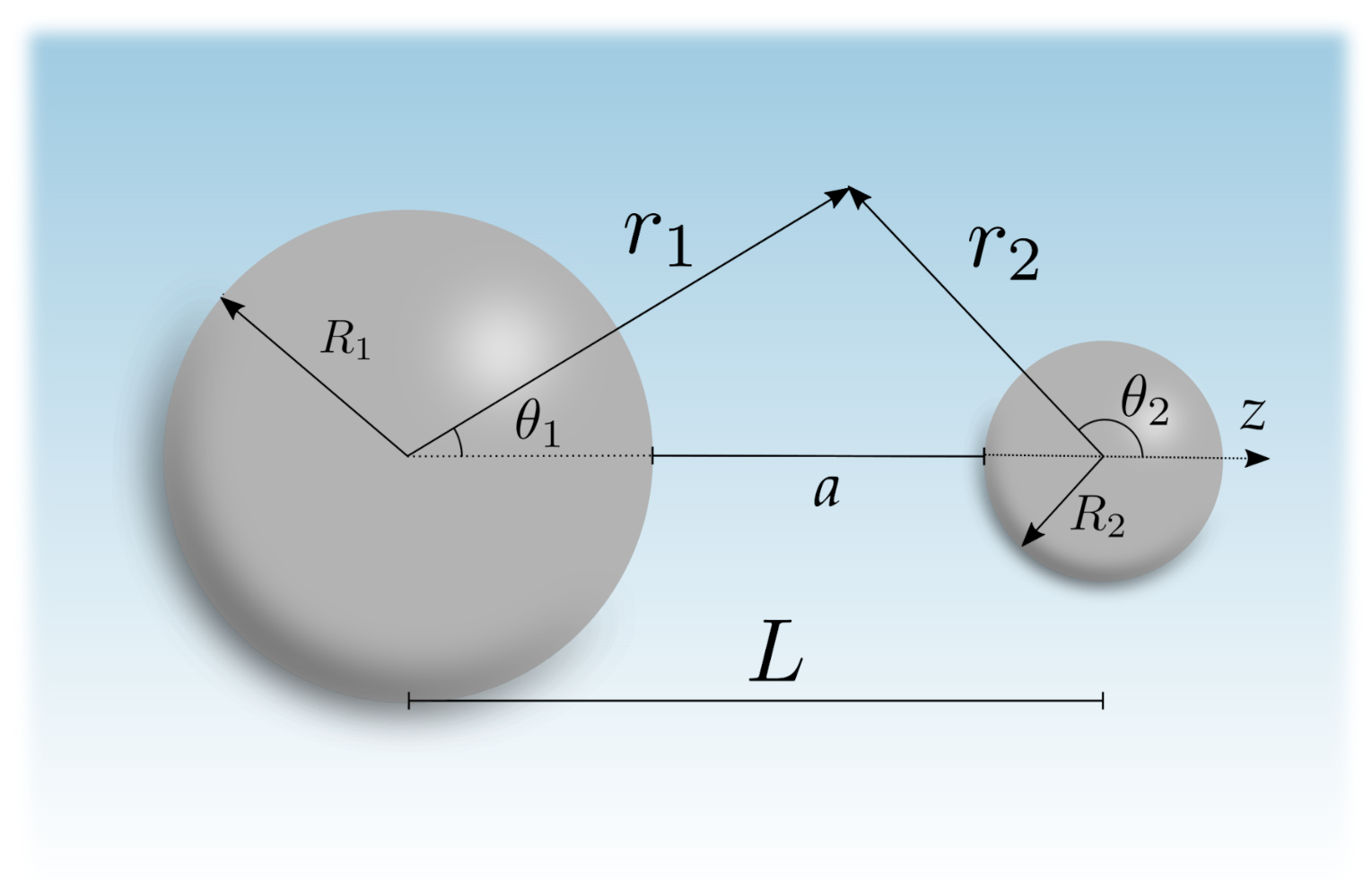
Our system consists of two solid spheres of radii $R_1$ and $R_2$, with permittivities ${ϵ}_1$ and ${ϵ}_2$, respectively, separated by a surface-to-surface distance $a,$ so that the distance between both centers is $L=a+R_1+R_2$ along the z axis; see Figure 1. The spheres are immersed in an electrolyte solution with a permittivity ${\mathit{ϵ}}_3$ and bulk ionic concentration $c_0$. Moreover, the whole system is in thermal equilibrium at a temperature T.

The Casimir free energy is given by [3,57]

$$\begin{array}{cc}\hfill {\mathcal{F}}_{\mathrm{cas}}\left(a\right)& =\frac{k_{B}T}{2}logD\left(i{\xi }_0\right)+k_{B}T\sum _{n=1}^{\infty }log\mathcal{D}\left(i{\xi }_n\right),\hfill \\ \hfill & ={\mathcal{F}}_{\mathrm{cas}}^0(a,{\lambda }_D)+{\mathcal{F}}_{\mathrm{cas}}^{n\ge 1}\left(a\right)\hfill \end{array}$$

(1)

where $k_B$ is the Boltzmann constant, and ${\xi }_n$ is the nth Matsubara frequency, given by ${\xi }_n=2\pi n{k}_{B}T/ħ$. The quantities $D\left(x\right)$ and $\mathcal{D}\left(x\right),$ to be defined later, are useful determinants that are connected to the (complex) mode structure of the system [15,16,66,67,68,69] for zero and finite frequencies, respectively.

The fact that the solid spheres are immersed in an electrolyte solution substantially complicates the problem, as the dissolved ions introduce spatial dispersion [54]. For realistic values of ion concentrations (and masses), however, the characteristic frequencies of the ionic individual and collective motions are much smaller than even the first nonzero Matsubara frequency ${\xi }_1$ [57]. As a consequence, one can show that the effect of the ions on the positive-frequency determinant $\mathcal{D}\left(i{\xi }_n\right)$ is negligible [58]. Therefore, we shall assume that only the zero-frequency determinant $D\left(i{\xi }_0\right)$ term in (1) “feels” the presence of the ions, while the $n\ge 1$ terms may be obtained by solving the scattering problem for a spatially local medium.

2.2. The n = 0 Contribution

For the zero-frequency contribution, we follow the electrostatic fluctuational approach [55,56,57] and derive the Casimir free energy from the solutions of the Laplace and linear Poisson-Boltzmann equations for the geometry of two spheres with no sources. Given that we have only charge fluctuations on the spheres, the expectation value of the potential is going to satisfy $e^2\langle {\psi }^2\rangle \lesssim {\left(k_{B}T\right)}^2$ within the electrolyte, which is just the condition for linearization [52]. When following the scattering approach for spatially-dispersive media, an additional contribution arises from transverse magnetic modes in the zero-frequency limit [58]. Experimental evidence for such contribution was recently reported [70]. Here, however, in order to calculate the $n=0$ contribution, we take the electrostatic limit from the start. Therefore, such additional contribution does not appear. In other words, we generalize the standard approach of Refs. [56,57] to the sphere-sphere geometry.

As mentioned in the previous section, our main task is to determine the mode structure of the system. Such undertaking is necessary due to the fact that, as we are dealing with thermal charge fluctuations, the potential may also fluctuate into all possible modes. In that spirit, we solve the Laplace equation for the electric potential $\psi \left(\mathbf{r}\right)$

$${\nabla }^2\psi \left(\mathbf{r}\right)=0,$$

(2)

where we used the fact that there are no free electric charges inside the spheres (i.e., the spheres are dielectric). Outside the spheres, in the electrolyte solution, the potential satisfies the linearized Poisson-Boltzmann equation [51]

$${\nabla }^2\psi \left(\mathbf{r}\right)={\kappa }_D^2\psi \left(\mathbf{r}\right),$$

(3)

where

$${\kappa }_D={\lambda }_D^{-1}=\sqrt{{\displaystyle \frac{2c_0{q}^2}{{ϵ}_3{k}_{B}T}}}$$

(4)

is the inverse of the Debye length ${\lambda }_D$, which is a measure of the diffuse double-layer thickness [51], and q is the absolute value of the charge of the ions.

In terms of a spherical coordinate system concentric to sphere 1, the solution of the Laplace equation inside sphere 1 is

$$\psi (r_1,{\theta }_1,{\varphi }_1)=\sum _{\ell =0}^{\infty }\sum _{m=-\ell }^{\ell }{c}_{\ell m}{r}_1^{\ell }{P}_{\ell }^m(cos{\theta }_1)e^{-im{\varphi }_1}{r}_1<R_1,$$

(5)

and, similarly, inside sphere 2, we have

$$\psi (r_2,{\theta }_2,{\varphi }_2)=\sum _{\ell =0}^{\infty }\sum _{m=-\ell }^{\ell }{d}_{\ell m}{r}_2^{\ell }{P}_{\ell }^m(cos{\theta }_2)e^{-im{\varphi }_2}{r}_2<R_2,$$

(6)

where the lengths $r_1$ and $r_2$ and the angles ${\theta }_1$ and ${\theta }_2$ are indicated in Figure 1. The coefficients $c_{\ell m}$ and $d_{\ell m}$ are determined by the boundary conditions at the spherical surfaces. We choose the line that connects the 2 centers as the z axis, so ${\varphi }_1={\varphi }_2=\varphi$ and $P_{\ell }^m$ are the associated Legendre polynomials [71].

Outside the spheres, we have to solve the linear Poisson-Boltzmann equation (3). It is also separable in spherical coordinates, and we write the solution $\psi \left(\mathbf{r}\right)$ for the sphere-sphere geometry as the superposition of contributions ${\psi }_1\left(\mathbf{r}\right)$, ${\psi }_2\left(\mathbf{r}\right)$ coming from each sphere

$$\begin{array}{cc}\hfill \psi \left(\mathbf{r}\right)& ={\psi }_1(r_1,{\theta }_1,{\varphi }_1)+{\psi }_2(r_2,{\theta }_2,{\varphi }_2)\hfill \\ \hfill & =\sum _{\ell =0}^{\infty }\sum _{m=-\ell }^{\ell }\left[a_{\ell m}{k}_{\ell }\left({\kappa }_D{r}_1\right)P_{\ell }^m(cos{\theta }_1)e^{-im\varphi }+b_{\ell m}{k}_{\ell }\left({\kappa }_D{r}_2\right)P_{\ell }^m(cos{\theta }_2)e^{-im\varphi }\right],\hfill \end{array}$$

(7)

where $k_{\ell }\left(x\right)$ is the modified spherical Bessel function of the second kind [71], and $a_{\ell m}$ and $b_{\ell m}$ are coefficients to be determined. Equation (7) does not imply that ψ₁ (ψ₂) may be understood as the potential of the sphere 1(2) in the absence of the other (although such interpretation would hold if κ_DL ≫ 1), as it is evidenced by the fact that all coefficients a_ℓm, b_ℓm, c_ℓm, d_ℓm depend on the boundary conditions imposed by the two spheres. Despite its relative simplicity, expression (7) is not convenient as it makes reference to two different (but interdependent) coordinate systems. In order to write the solution (7) in terms of a single coordinate system, we use an important spherical addition theorem [62] and arrive at

$$\begin{array}{cc}\hfill \psi (r_1,{\theta }_1,\varphi )& =\sum _{\ell =0}^{\infty }\sum _{m=-\ell }^{\ell }{e}^{-im\varphi }[a_{\ell m}{k}_{\ell }\left({\kappa }_D{r}_1\right)P_{\ell }^m(cos{\theta }_1)\hfill \\ & \phantom{=\sum _{\ell =0}^{\infty }\sum _{m=-\ell }^{\ell }{e}^{-im\varphi }[}+b_{\ell m}\sum _{n=m}^{\infty }(2n+1)\frac{(n-m)!}{(n+m)!}{U}_{\ell n}^m\left({\kappa }_{D}L\right)i_n\left({\kappa }_D{r}_1\right)P_n^m(cos{\theta }_1)],\hfill \end{array}$$

(8)

$$\begin{array}{cc}\hfill \psi (r_2,{\theta }_2,\varphi )& =\sum _{\ell =0}^{\infty }\sum _{m=-\ell }^{\ell }{e}^{-im\varphi }[a_{\ell m}\sum _{n=m}^{\infty }(2n+1)\frac{(n-m)!}{(n+m)!}{U}_{\ell n}^m\left({\kappa }_{D}L\right)i_n\left({\kappa }_D{r}_2\right)P_n^m(cos{\theta }_2)\hfill \\ & \phantom{=\sum _{\ell =0}^{\infty }\sum _{m=-\ell }^{\ell }{e}^{-im\varphi }[}+b_{\ell m}{k}_{\ell }\left({\kappa }_D{r}_2\right)P_{\ell }^m(cos{\theta }_2)],\hfill \end{array}$$

(9)

where $i_n\left(x\right)$ is the modified spherical Bessel function of the first kind [71], and $U_{ln}^m\left(c\right)$ is given by

$$\begin{array}{cc}\hfill U_{\ell n}^m\left(c\right)& ={\left(\frac{2}{c}\right)}^m\sum _{\nu =0}^{\ell -m}\frac{\Gamma (\ell -\nu +\frac{1}{2})\Gamma (n-\nu +\frac{1}{2})\Gamma (m+\nu +\frac{1}{2})}{\Gamma (\ell +n-m-\nu +\frac{3}{2})\Gamma (m+\frac{1}{2})\pi }\hfill \\ \hfill & \phantom{={\left(\frac{2}{c}\right)}^m\sum _{\nu =0}^{\ell -m}}\times \frac{(\ell +n-\nu )!(\ell +n-m-2\nu +\frac{1}{2})}{(\ell -m-\nu )!(n-m-\nu )!\nu !}{k}_{\ell +n-m-2\nu }\left(c\right),\hfill \end{array}$$

(10)

where, $\Gamma \left(x\right)$ denotes the gamma function [71]. Note that $U_{ln}^m$ was derived for spherical Bessel functions j_n(x) and y_n(x) in [62], and it differs from our formula for modified Bessel functions i_n(x) and k_n(x) by the pre-factor ${(-1)}^{\nu }$.

In order to determine the mode structure of the problem, we still have to apply the boundary conditions on both spherical surfaces. The continuity of the potential

$${\left.\psi (r_s,{\theta }_s)\right|}_{R_s^{-}}={\left.\psi (r_s,{\theta }_s)\right|}_{R_s^{+}},$$

(11)

leads us to two equations, where $s=1,2$. Combining Equations (5) and (8) for sphere 1 and Equations (6) and (9) for sphere 2, using the orthogonality of associated Legendre polynomials, and exploiting the rotational symmetry around z-axis, we can decompose Equation (11) into matrix equations for each azimuthal number m

$$\begin{array}{ccc}\hfill {\mathbb{S}}_1·\mathbf{c}& =& {\mathbb{K}}_1·\mathbf{a}+{\mathbb{B}}_{1m}·\mathbf{b},\hfill \end{array}$$

(12)

$$\begin{array}{ccc}\hfill {\mathbb{S}}_2·\mathbf{d}& =& {\mathbb{K}}_2·\mathbf{b}+{\mathbb{B}}_{2m}·\mathbf{a},\hfill \end{array}$$

(13)

where the column vector $\mathbf{a}$ contains the coefficients $a_{\ell m}$ with $\ell =m,m+1,m+2,...$ for fixed m and likewise for the column vectors $\mathbf{b},$$\mathbf{c},$ and $\mathbf{d}.$ The matrices appearing in Equations (12) and (13) are given by

$$\begin{array}{c}{\left({\mathbb{S}}_s\right)}_{\ell n}=R_s^{\ell }{\delta }_{n\ell },{\left({\mathbb{K}}_s\right)}_{\ell n}=k_n\left({\kappa }_D{R}_s\right){\delta }_{n\ell }\\ {\left({\mathbb{B}}_{sm}\right)}_{\ell n}=(2n+1)\frac{(n-m)!}{(n+m)!}{U}_{\ell n}^m\left({\kappa }_{D}L\right)i_n\left({\kappa }_D{R}_s\right).\end{array}$$

(14)

The continuity of the electric displacement radial component

$${ϵ}_s{\left.\frac{\partial \psi }{\partial r}\right|}_{R_s^{-}}={ϵ}_3{\left.\frac{\partial \psi }{\partial r}\right|}_{R_s^{+}}$$

(15)

also leads us to matrix equations

$$\begin{array}{ccc}\hfill {\mathbb{S}}_1^{{}^{\prime }}·\mathbf{c}& =& {\mathbb{K}}_1^{{}^{\prime }}·\mathbf{a}+{\mathbb{B}}_{1m}^{{}^{\prime }}·\mathbf{b},\hfill \end{array}$$

(16)

$$\begin{array}{ccc}\hfill {\mathbb{S}}_2^{{}^{\prime }}·\mathbf{d}& =& {\mathbb{K}}_2^{{}^{\prime }}·\mathbf{b}+{\mathbb{B}}_{2m}^{{}^{\prime }}·\mathbf{a}.\hfill \end{array}$$

(17)

The matrices appearing above are defined by

$$\begin{array}{c}{\left({\mathbb{S}}_s^{\prime }\right)}_{\ell n}={ϵ}_s\ell R_s^{\ell -1}{\delta }_{n\ell },{\left({\mathbb{K}}_s^{\prime }\right)}_{\ell n}={ϵ}_3{\kappa }_D{k}_n^{\prime }\left({\kappa }_D{R}_s\right){\delta }_{n\ell }\\ {\left({\mathbb{B}}_{sm}^{\prime }\right)}_{\ell n}={ϵ}_3{\kappa }_D(2n+1)\frac{(n-m)!}{(n+m)!}{U}_{\ell n}^m\left({\kappa }_{D}L\right)i_n^{\prime }\left({\kappa }_D{R}_s\right),\end{array}$$

(18)

where the prime on Bessel functions indicates differentiation with respect to the argument.

For each m, Equations (12), (13), (16), and (17) form a homogeneous (infinite) system, as it could be anticipated given that there are no external sources (in particular, the spheres are not charged). As such, nontrivial solutions are possible if and only if the determinants of the coefficient matrices vanish, leading us to the condition

$$\det \left[𝟙-{\mathbb{R}}_1{\mathbb{T}}_m{\mathbb{R}}_2{\mathbb{T}}_m\right]=0,(m\in \mathbb{Z}),$$

(19)

where $𝟙$ is the identity matrix, and the scattering and propagation matrices, ${\mathbb{R}}_s$ and ${\mathbb{T}}_m,$ respectively, are given by

$${\left({\mathbb{R}}_s\right)}_{\ell n}=\frac{\frac{{ϵ}_3}{{ϵ}_s}{\kappa }_D{R}_s{i}_n^{\prime }\left({\kappa }_D{R}_s\right)-\ell i_n\left({\kappa }_D{R}_s\right)}{\frac{{ϵ}_3}{{ϵ}_s}{\kappa }_D{R}_s{k}_n^{\prime }\left({\kappa }_D{R}_s\right)-\ell k_n\left({\kappa }_D{R}_s\right)}{\delta }_{\ell n},$$

(20)

and

$${\left({\mathbb{T}}_m\right)}_{\ell n}=(2n+1)\frac{(n-m)!}{(n+m)!}{U}_{\ell n}^m\left({\kappa }_{D}L\right).$$

(21)

The full structure of solutions for this system is then determined by

$$\prod _{m=-\infty }^{\infty }\det \left[𝟙-{\mathbb{R}}_1{\mathbb{T}}_m{\mathbb{R}}_2{\mathbb{T}}_m\right]=0,(m\in \mathbb{Z}).$$

(22)

In other words, we see that Equation (22) characterizes the normal modes of the setup. This is auspicious because, according to the prescription outlined in References [56,57,66], that is precisely what we need in order to compute the zero-frequency contribution to the Casimir energy: the function $D\left(i{\xi }_0\right)$ introduced in Equation (1) is to be identified with the l.h.s of (22). At this point, it is worth emphasizing that we are not solving the normal-mode problem per se, we just need the equation that defines such modes. Therefore, we find

$$\begin{array}{cc}\hfill {\mathcal{F}}_{\mathrm{cas}}^0(a,{\lambda }_D)& =\frac{k_{B}T}{2}logD\left(i{\xi }_0\right)\hfill \\ \hfill & =\frac{k_{B}T}{2}\sum _{m=-\infty }^{\infty }log\det \left[𝟙-{\mathbb{R}}_1{\mathbb{T}}_m{\mathbb{R}}_2{\mathbb{T}}_m\right].\hfill \end{array}$$

(23)

2.3. The $n\ge 1$ Contributions

As indicated in the end of Section 2.1, the contributions to the Casimir free energy coming from finite Matsubara frequencies are to be obtained from the scattering approach [15,16] by neglecting the presence of the ions. For two spheres, the Casimir free energy can be found from Equation (1) with

$$\mathcal{D}\left(i{\xi }_n\right)=\det (1-\mathcal{M}\left(i{\xi }_n\right)),$$

(24)

where the round-trip operator is defined as

$$\mathcal{M}={\mathcal{T}}_{12}{\mathcal{R}}_2{\mathcal{T}}_{21}{\mathcal{R}}_1.$$

(25)

Here, ${\mathcal{R}}_s$ denotes the reflection operator at sphere $s=1,2$ with the coordinate system being centered at the respective sphere, and ${\mathcal{T}}_{21}$ stands for the translation operator from the center of sphere 1 to center of sphere 2, and vice versa for ${\mathcal{T}}_{12}$.

Note that, because of the determinant in (24), we are free to choose a basis for the electromagnetic modes in which the round-trip operator and its constituents are to be expanded. Here, we follow the plane-wave numerical approach presented in Reference [59], as it shows far better convergence rates as compared to the commonly employed approach based on spherical multipoles [18,72]. In the following, we outline this plane-wave numerical approach for the geometry of two spheres.

2.3.1. Plane-Wave Representation

Within the angular spectrum representation, we denote the plane-wave basis elements by the kets $|\mathbf{k},\varphi ,p\rangle$ with the wavevector component perpendicular to the z-axis $\mathbf{k}$, the propagation direction relative to the z-axis $\varphi =\pm$ and $p=\mathrm{TM},\mathrm{TE}$ for transverse magnetic and transverse electric polarizations, respectively. As the frequency is conserved through the round trip, we suppress it in our notation.

While the round-trip operator is expressed as an infinite but discrete matrix when expanded in the multipolar basis, the round-trip operator is a continuous matrix when using plane-waves. Formally, the round-trip operator is then described as an integral operator:

$$\mathcal{M}|\mathbf{k},-,p\rangle =\sum _{p^{\prime }}\int \frac{\mathrm{d}{\mathbf{k}}^{\prime }}{{\left(2\pi \right)}^2}{f}_{\mathcal{M}}({\mathbf{k}}^{\prime },p^{\prime };\mathbf{k},p)|{\mathbf{k}}^{\prime },-,p^{\prime }\rangle ,$$

(26)

with the scalar kernel function $f_{\mathcal{M}}$.

The kernel function of the round-trip operator $f_{\mathcal{M}}$ can be expressed in terms of the kernel functions of its constituent operators. The translation operators are diagonal in the plane-wave basis with kernel functions

$$f_{{\mathcal{T}}_{21}}({\mathbf{k}}^{\prime },p^{\prime };\mathbf{k},p)=f_{{\mathcal{T}}_{12}}({\mathbf{k}}^{\prime },p^{\prime };\mathbf{k},p)={\left(2\pi \right)}^2{e}^{-\kappa L}{\delta }_{p,p^{\prime }}\delta (\mathbf{k}-{\mathbf{k}}^{\prime }),$$

(27)

where

$$\kappa =\sqrt{K^2+{\mathbf{k}}^2},$$

(28)

with the imaginary wave number $K=\sqrt{{ϵ}_3}{\xi }_n/c$ and the speed of light in vacuum c. The kernel function of the round-trip operator can then be expressed as

$$f_{\mathcal{M}}({\mathbf{k}}^{\prime },p^{\prime };\mathbf{k},p)=e^{-{\kappa }^{\prime }L}\sum _{p^{″}}\int \frac{\mathrm{d}{\mathbf{k}}^{″}}{{\left(2\pi \right)}^2}{f}_{{\mathcal{R}}_2}({\mathbf{k}}^{\prime },p^{\prime };{\mathbf{k}}^{″},p^{″})e^{-{\kappa }^{″}L}{f}_{{\mathcal{R}}_1}({\mathbf{k}}^{″},p^{″};\mathbf{k},p).$$

(29)

with ${\kappa }^{\prime }$ and ${\kappa }^{″}$ being defined as in (28). The summation and integration over the double primed variables (29) take all intermediate scattering channels between the two spheres into account.

The kernel function of the reflection operators for the spheres is given by [73,74]

$$\begin{array}{cc}\hfill f_{{\mathcal{R}}_s}({\mathbf{k}}^{\prime },\mathrm{TM};\mathbf{k},\mathrm{TM})& =\frac{2\pi }{K{\kappa }^{\prime }}(A{S}_2+B{S}_1)\hfill \\ \hfill f_{{\mathcal{R}}_s}({\mathbf{k}}^{\prime },\mathrm{TE};\mathbf{k},\mathrm{TE})& =\frac{2\pi }{K{\kappa }^{\prime }}(A{S}_1+B{S}_2)\hfill \\ \hfill f_{{\mathcal{R}}_s}({\mathbf{k}}^{\prime },\mathrm{TM};\mathbf{k},\mathrm{TE})& =-\frac{2\pi }{K{\kappa }^{\prime }}(C_s{S}_1+D_s{S}_2)\hfill \\ \hfill f_{{\mathcal{R}}_s}({\mathbf{k}}^{\prime },\mathrm{TE};\mathbf{k},\mathrm{TM})& =\frac{2\pi }{K{\kappa }^{\prime }}(C_s{S}_2+D_s{S}_1),\hfill \end{array}$$

(30)

with the plane-wave Mie scattering amplitudes [75]

$$\begin{array}{cc}\hfill S_1& =\sum _{\ell =1}^{\infty }\frac{2\ell +1}{\ell (\ell +1)}\left[a_{\ell }\left(iK{R}_s\right){\pi }_{\ell }(cos(\Theta ))+b_{\ell }\left(iK{R}_s\right){\tau }_{\ell }(cos(\Theta ))\right]\hfill \\ \hfill S_2& =\sum _{\ell =1}^{\infty }\frac{2\ell +1}{\ell (\ell +1)}\left[a_{\ell }\left(iK{R}_s\right){\tau }_{\ell }(cos(\Theta ))+b_{\ell }\left(iK{R}_s\right){\pi }_{\ell }(cos(\Theta ))\right],\hfill \end{array}$$

(31)

which depend on the electromagnetic response of the homogeneous spheres through the electric and magnetic Mie coefficients $a_{\ell }$ and $b_{\ell }$, respectively [75]. The angular functions ${\pi }_{\ell }$ and ${\tau }_{\ell }$ appearing in (31) are defined as [75]

$$\begin{array}{cc}\hfill {\pi }_{\ell }\left(z\right)& =P_{\ell }^{\prime }\left(z\right)\hfill \\ \hfill {\tau }_{\ell }\left(z\right)& =-(1-z^2)P_{\ell }^{″}\left(z\right)+z{P}_{\ell }^{\prime }\left(z\right),\hfill \end{array}$$

(32)

where $P_{\ell }\left(z\right)$ denotes a Legendre polynomial [71]. The angular functions only depend on the scattering angle $\Theta$, which is expressed as

$$cos\mathrm{\Theta }=-\frac{\mathbf{k}·{\mathbf{k}}^{\prime }+\kappa {\kappa }^{\prime }}{K^2}.$$

(33)

The functions A, B, $C_s$, and $D_s$ in (30) describe a rotation from the polarization basis defined through the scattering plane to the TE-TM polarization basis. They are functions of the incident and scattered wave vectors and can be expressed as [73]

$$\begin{array}{cc}\hfill A& =\frac{K^{4}cos\left(\mathrm{\Delta }\phi \right)-[k{k}^{\prime }cos\left(\mathrm{\Delta }\phi \right)-\kappa {\kappa }^{\prime }][k{k}^{\prime }-\kappa {\kappa }^{\prime }cos\left(\mathrm{\Delta }\phi \right)]}{K^4-{[k{k}^{\prime }cos\left(\mathrm{\Delta }\phi \right)-\kappa {\kappa }^{\prime }]}^2},\hfill \\ \hfill B& =-\frac{K^{2}k{k}^{\prime }{sin}^2\left(\mathrm{\Delta }\phi \right)}{K^4-{[k{k}^{\prime }cos\left(\mathrm{\Delta }\phi \right)-\kappa {\kappa }^{\prime }]}^2},\hfill \\ \hfill C_s& ={(-1)}^{s}Ksin\left(\mathrm{\Delta }\phi \right)\frac{k{k}^{\prime }\kappa cos\left(\mathrm{\Delta }\phi \right)+k^2{\kappa }^{\prime }}{K^4-{[k{k}^{\prime }cos\left(\mathrm{\Delta }\phi \right)-\kappa {\kappa }^{\prime }]}^2},\hfill \\ \hfill D_s& ={(-1)}^{s+1}Ksin\left(\mathrm{\Delta }\phi \right)\frac{k{k}^{\prime }{\kappa }^{\prime }cos\left(\mathrm{\Delta }\phi \right)+{k^{\prime }}^2\kappa }{K^4-{[k{k}^{\prime }cos\left(\mathrm{\Delta }\phi \right)-\kappa {\kappa }^{\prime }]}^2},\hfill \end{array}$$

(34)

where we have employed polar coordinates $\mathbf{k}=(k,\phi )$ and ${\mathbf{k}}^{\prime }=(k^{\prime },{\phi }^{\prime })$, and $\mathrm{\Delta }\phi ={\phi }^{\prime }-\phi$. Note that the signs in the functions $C_s$ and $D_s$ for sphere s reflect the orientation of the z-axis. They are different for the two spheres as the plane-wave propagation direction with respect to the z-axis changes from $\varphi =-$ to ${\varphi }^{\prime }=+$ upon reflection on sphere 1, and vice versa for sphere 2.

2.3.2. Numerical Application

For a numerical evaluation of (24), a discretization of the continuous wave vectors is required. In order to exploit the cylindrical symmetry of the problem, we employ polar coordinates $\mathbf{k}=(k,\phi )$. The two integrals over radial and angular components of the transverse wave vector ${\mathbf{k}}^{\prime }$ in (26) can then be discretized using one-dimensional quadrature rules. Denoting the quadrature nodes and weights for the radial and angular components as $(k_{i^{\prime }},w_{i^{\prime }})$ for $i^{\prime }=1,\dots ,N^{\prime }$ and $({\phi }_{j^{\prime }},v_{j^{\prime }})$ for $j^{\prime }=1,\dots ,M^{\prime }$, respectively, we can express (26) in discretized form as

$$\mathcal{M}|k_i,{\phi }_j,-,p\rangle =\sum _{p^{\prime }=\mathrm{TM},\mathrm{TE}}\sum _{i^{\prime }=1}^{N^{\prime }}\sum _{j^{\prime }=1}^{M^{\prime }}\frac{k_{i^{\prime }}{w}_{i^{\prime }}{v}_{j^{\prime }}}{{\left(2\pi \right)}^2}{f}_{\mathcal{M}}(k_{i^{\prime }},{\phi }_{j^{\prime }},p^{\prime };k_i,{\phi }_j,p)|k_{i^{\prime }},{\phi }_{j^{\prime }},-,p^{\prime }\rangle$$

(35)

for $i=1,\dots ,N^{\prime }$, $j=1,\dots ,M^{\prime }$ and $p=\mathrm{TE},\mathrm{TM}$. Consequently, the discretized matrix elements of the round-trip operator read [76]

$$\langle k_{i^{\prime }}{\phi }_{j^{\prime }},-,p^{\prime }\left|\mathcal{M}\right|k_i,{\phi }_j,-,p\rangle =\frac{k_{i^{\prime }}{w}_{i^{\prime }}{v}_{j^{\prime }}}{{\left(2\pi \right)}^2}{f}_{\mathcal{M}}(k_{i^{\prime }},{\phi }_{j^{\prime }},p^{\prime };k_i,{\phi }_j,p).$$

(36)

Applying the same discretization procedure to the integral appearing in (29), the threefold block matrix (36) can be expressed as the product of block matrices

$$\langle k_{i^{\prime }},{\phi }_{j^{\prime }},-,p^{\prime }\left|\mathcal{M}\right|k_i,{\phi }_j,-,p\rangle =\sum _{p^{″}=\mathrm{TM},\mathrm{TE}}\sum _{i^{″}=1}^{N^{″}}\sum _{j^{″}=1}^{M^{″}}{\left({\mathbb{X}}_2\right)}_{i^{\prime },j^{\prime },p^{\prime };i^{″},j^{″},p^{″}}{\left({\mathbb{X}}_1\right)}_{i^{″},j^{″},p^{″};i,j,p},$$

(37)

with

$${\left({\mathbb{X}}_s\right)}_{i^{\prime },j^{\prime },p^{\prime };i,j,p}=\frac{k_{i^{\prime }}{w}_{i^{\prime }}{v}_{j^{\prime }}}{{\left(2\pi \right)}^2}exp\left(-L\sqrt{K^2+k_{i^{\prime }}^2}\right)f_{{\mathcal{R}}_s}(k_{i^{\prime }},{\phi }_{j^{\prime }},p^{\prime };k_i,{\phi }_j,p)$$

(38)

describing the reflection on sphere s followed by a translation to the other sphere. Note that the discretization orders for the radial components of the wave vectors $N^{\prime }$ and $N^{″}$ are not required to be the same. Thus, the ${\mathbb{X}}_s$ are in general rectangular matrices. As we will discuss below, in order to exploit the cylindrical symmetry of the problem, it will, however, be required that $M^{\prime }=M^{″}$ for the angular discretization orders.

The Casimir energy can now be numerically computed by replacing the round-trip operator in (24) with the corresponding finite matrix (37). While, in principle, one is free to choose quadrature rules, we found those specified in the following particularly suited for the problem at hand [59].

For the radial component, we employ the Fourier-Chebyshev quadrature rule introduced in Reference [77]. With

$$t_i=\frac{\pi i}{N^{\prime }+1},$$

(39)

the quadrature rule is specified by its nodes

$$k_i=b{cot}^2(t_i/2)$$

(40)

and weights

$$w_i=\frac{8bsin\left(t_i\right)}{{[1-cos\left(t_i\right)]}^2}\frac{1}{N^{\prime }+1}\sum _{\begin{array}{c}j=1\\ j\mathrm{odd}\end{array}}^{N^{\prime }}\frac{sin\left(j{t}_i\right)}{j}$$

(41)

for $i=1,\cdots ,N^{\prime }$. An optimal choice for the free parameter b can boost the convergence of the computation. For dimensional reasons, the transverse wave vector and, thus, b should scale like the inverse surface-to-surface distance $1/a$. In fact, the choice $b=1/a$ already yields a fast convergence rate as has been demonstrated in Reference [59].

For the angular component of the transverse wave vectors, we employ the trapezoidal quadrature rule. Its nodes and weights are defined by ${\phi }_j=2\pi j/M^{\prime }$ and $v_j=2\pi /M^{\prime }$, respectively, for $j=1,\dots ,M^{\prime }$. While, for arbitrary functions, the trapezoidal rule is not efficient, it is exponentially convergent for periodic functions appearing here.

Moreover, the trapezoidal rule allows us to further exploit the cylindrical symmetry of the problem. Note that, due to the cylindrical symmetry, the kernel function of the reflection operator on the spheres (30), and, thus, also the kernel function of the round-trip operator (29), depend only on the difference $\mathrm{\Delta }\phi ={\phi }^{\prime }-\phi$ of angular components. Using the trapezoidal rule, the discretized matrix elements (36) then only depend on the difference of indices $j^{\prime }-j$. A square block matrix of this form is known as circulant block matrix. It is well-known that a circulant block matrix can be block diagonalized using a discrete Fourier transform. If we choose $M^{\prime }=M^{″}$ for the angular discretization orders, the discretized round-trip operator (37) can be expressed as a product of block-diagonal matrices. In this block-diagonal form, the determinant (24) factorizes, thus reducing the computational complexity of the problem.

In fact, the indices labeling the diagonal blocks after the discrete Fourier transform can then be identified with the angular indices $m,$ known from the spherical multipole representation, which denote the axial component of the electromagnetic field angular momentum. Particularly at short distances, the plane-wave basis is advantageous with respect to the spherical multipole basis because the required size of the block matrices is considerably smaller as the following estimate demonstrates. The size of the diagonal blocks of ${\mathbb{X}}_2$ and ${\mathbb{X}}_1$ appearing in (37) is determined by the radial quadrature orders $N^{\prime }$ and $N^{″}$ in the plane-wave representation. In particular, they are of shape $2N^{\prime }\times 2N^{″}$ and $2N^{″}\times 2N^{\prime }$, respectively, where the factor of 2 is due to the two polarization components. It can be shown that, in order to maintain a certain numerical error for short separations $a\ll R_1,R_2$, the discretization orders need to scale as $N^{\prime }\sim \sqrt{R_{\mathrm{eff}}/a}$ and $N^{″}\sim \sqrt{(R_1+R_2)/a}$ with the effective radius $R_{\mathrm{eff}}=R_1{R}_2/(R_1+R_2)$ [59]. On the other hand, within the spherical multipole representation, the block matrix sizes are determined by the highest multipole index ${\ell }_{\max }$ included in the calculation, which scales linearly in $R_1/a$ and $R_2/a$ [72,78,79].

3. Results and Discussion

3.1. Numerical Considerations

By symmetry, the contribution of the m-th term in Equation (23) does not depend on the sign of $m,$ which allows one to replace (23) by a sum over non-negative values only. In the spherical-wave basis, it turns out that the round-trip operator in the form ${\mathbb{R}}_1{\mathbb{T}}_m{\mathbb{R}}_2{\mathbb{T}}_m$ is ill-conditioned with exponentially increasing and decreasing matrix elements in the off-diagonal corners. For numerical purposes, it has proven advantageous to use an equivalent symmetrized form of the round-trip operator instead which leads to a diagonally dominant matrix [9,10]. Equation (23) then reads

$${\mathcal{F}}_{\mathrm{cas}}^0(a,{\lambda }_D)=k_{B}T\sum _{m=0}^{\infty }{}^{{}^{\prime }}log\det \left[𝟙-\sqrt{{\mathbb{R}}_1}{\mathbb{T}}_m{\mathbb{R}}_2{\mathbb{T}}_m\sqrt{{\mathbb{R}}_1}\right].$$

(42)

Taking the square root of the reflection operator at sphere 1 does not present any difficulties, particularly in the spherical-wave basis, where its matrix representation is diagonal. The primed sum in (42) indicates that the $m=0$ term is multiplied by $1/2.$

The matrices in the previous equation have in principle infinitely many components, so we need an effective truncation strategy. The size of the matrices appearing in Equation (42) is directly related to the highest multipole order ${\ell }_{\max }\sim R_s/a$ required for convergence [72,78,79]. The dimension of the matrix corresponding to the $(m+1)$-th term in (42) is ${\ell }_{\max }-{\ell }_{\min }$, where ${\ell }_{\min }=m,$ and the sum over m is truncated at ${\ell }_{\max }$.

3.2. The Screening Effect

For the numerical calculations, we choose either two polystyrene (PS) or silica (SiO${}_2$) spheres immersed in an aqueous electrolyte solution. In all numerical examples, we assume $R_1=R_2$ ($=1\mathsf{\mu }\mathrm{m}$ in the examples with PS) but our formalism also applies to the geometry with different radii. We take ${ϵ}_{\mathrm{PS}}\left(0\right)=2.37,$ ${ϵ}_{{\mathrm{SiO}}_2}\left(0\right)=3.91,$ and ${ϵ}_{{\mathrm{H}}_2\mathrm{O}}\left(0\right)=78.70$ for the static relative permitivities of PS, silica and water, respectively. For finite frequencies, we use a Drude-Lorentz model of N oscillators

$$ϵ\left(i\xi \right)=1+\sum _{i=1}^N\frac{C_i}{1+{\xi }^2/{\omega }_i^2},$$

(43)

with data for the parameters $C_i$ and ${\omega }_i$ taken from Reference [49] for both PS and water. Finally, we assume that the ions are monovalent ($q\approx 1.6\times {10}^{-19}$ C is the elementary charge) and that $T=293$ K.

We calculate the Casimir force by taking the derivative of the Casimir free energy

$$F_{\mathrm{cas}}(a,{\lambda }_D)=-\frac{\partial {\mathcal{F}}_{\mathrm{cas}}}{\partial a}$$

(44)

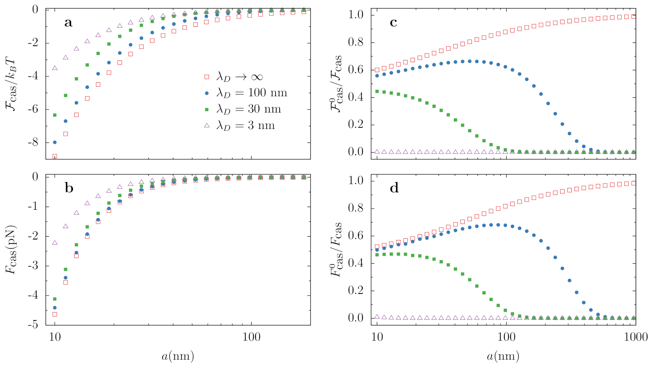
and show the variation of the Casimir energy and force with the distance a in Figure 2a,b, respectively, for different ionic concentrations. The curves confirm the rather intuitive behavior that, as we enhance the ion concentration, the force decreases due to the progressive screening of the zeroth frequency contribution. We also show (squares) the results for vanishing salt concentration (${\lambda }_D\to \infty ),$ which coincides with the standard Casimir calculation disregarding the effect of ions. Note, however, that the Debye length is theoretically limited to $\sim 1$ μm due to the spontaneous dissociation of the water molecule itself [51], and actual reported values of ${\lambda }_D$ are typically much smaller than that, even when no salt is added to the sample (see, for instance, Reference [80]). We are now in a good position to critically assess how accurate are [59] two widely used limits: (i) no screening (${\lambda }_D\to \infty$), where the zeroth term comes from the “standard” spherical Casimir calculation [16,72], and (ii) complete screening, where the zeroth contribution is simply neglected. The latter case is well approximated, for the distance interval shown in Figure 2, by the case ${\lambda }_D=3\mathrm{nm}$ (triangles).

We plot the relative contribution of the zeroth frequency term to the total result, for both the Casimir energy and the Casimir force in Figure 2 (plots c and d, respectively). We see that, when unscreened, the relative contribution of $F_{\mathrm{cas}}^0$ is always larger than 50% from 10 nm onwards. This is a consequence of the low contrast between the permittivities of polystyrene and water for finite Matsubara frequencies and tells us that an assessment of the screening is quantitatively very important. As we increase the ion concentration, the zeroth contribution gets more and more screened, but, even for $a\approx 2{\lambda }_D$, i.e., with considerable screening by the ions, and ${\lambda }_D=100\mathrm{nm}$ (circles), it still contributes ∼50% of the total force. It is true that the absolute values for the force are rather small in this range, but they are still within reach of measurements using optical tweezers [70,81,82,83,84,85].

3.3. Zero-Frequency Contribution for Very Small Spheres.

In this subsection, we derive a simple analytical result for very small spheres, $R_1,R_2\ll L$, as a limit of the general result (23). We focus here on the zero-frequency contribution, which is the one affected by screening. For that purpose, it is convenient to use the well known relation $log\det M=\mathrm{tr}logM$, valid for a generic matrix M, to write

$$\begin{array}{cc}\hfill {\mathcal{F}}_{\mathrm{cas}}^0& \approx \frac{k_{B}T}{2}\sum _{m=-\infty }^{\infty }\mathrm{tr}\left[{\mathbb{R}}_1{\mathbb{T}}_m{\mathbb{R}}_2{\mathbb{T}}_m\right]\hfill \\ \hfill & \approx \frac{k_{B}T}{2}\sum _{m=-1}^1\mathrm{tr}\left[{\mathbb{R}}_1{\mathbb{T}}_m{\mathbb{R}}_2{\mathbb{T}}_m\right].\hfill \end{array}$$

(45)

The sequence of approximations is consistent with the fact that we retain only the leading-order terms on $R_1{R}_2$ in the summation, which in this case turn out to be $\sim {\left(R_1{R}_2\right)}^3$. The explicit result is

$$\begin{array}{cc}\hfill {\mathcal{F}}_{\mathrm{cas}}^0& =-{\displaystyle \frac{k_{B}T{\kappa }_D^6}{2}}{e}^{-2{\kappa }_{D}L}[\frac{1}{9{\kappa }_D^2{L}^2}{R}_1^3{R}_2^3-{\displaystyle \frac{{(1+{\kappa }_{D}L)}^2}{3{\kappa }_D^4{L}^4}}({\alpha }_1{R}_2^3+{\alpha }_2{R}_1^3)\hfill \\ \hfill & \phantom{=-{\displaystyle \frac{k_{B}T{\kappa }_D^6}{2}}{e}^{-2{\kappa }_{D}L}[}+(6+12{\kappa }_{D}L+10{\kappa }_D^2{L}^2+4{\kappa }_D^3{L}^3+{\kappa }_D^4{L}^4){\displaystyle \frac{{\alpha }_1{\alpha }_2}{{\left({\kappa }_{D}L\right)}^6}}],\hfill \end{array}$$

(46)

where

$${\alpha }_s={\displaystyle \frac{({ϵ}_s-{ϵ}_3)}{({ϵ}_s+2{ϵ}_3)}}{R}_s^3$$

(47)

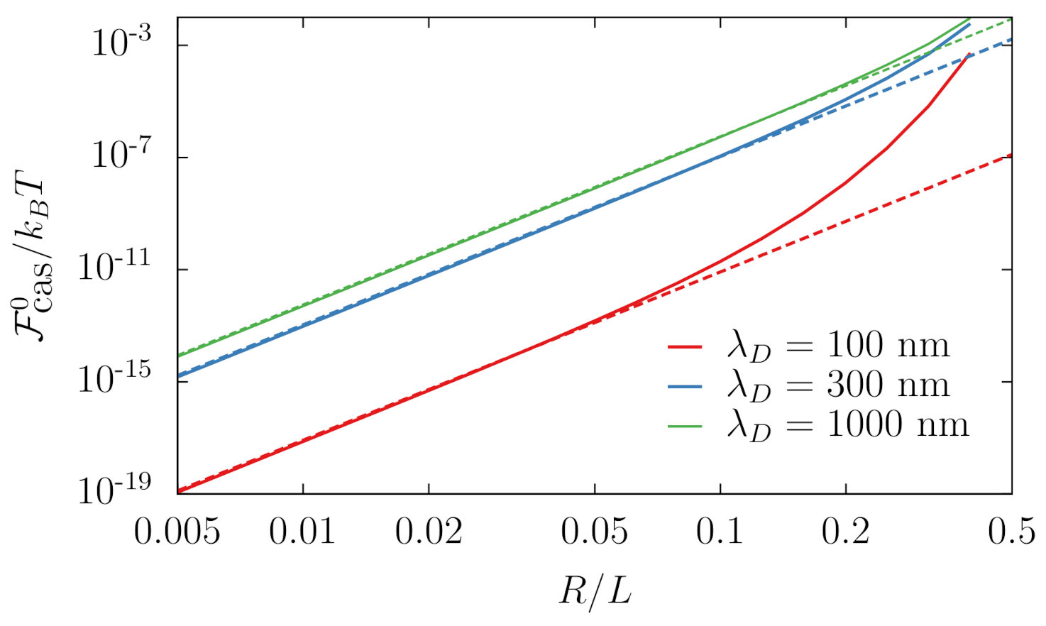
is the electric polarizability of sphere s. The third parcel in (46) reproduces exactly a result by Mahanty and Ninham [56] for fluctuating dipoles in an electrolyte solution, but we also obtain extra terms even at the lowest order in $R_1{R}_2$. These terms have an extremely suggestive form and, as we shall see in the following subsection, it is very reasonable to associate them to monopole-monopole and monopole-dipole fluctuation interactions [57]. Moreover, such interpretation in terms of multipoles is certainly consistent with Figure 3, where we depict the Casimir free energy between two identical silica spheres for different Debye lengths. One can clearly see that the small radii limit establishes itself at $2R\lesssim {\lambda }_D$, which is reasonable: when the object is much smaller than the diffuse layer of ions surrounding it, its shape is unimportant; therefore, the first multipole contributions should dominate the interaction. On the other hand, when the object’s dimensions are comparable to its screening region, the latter is deformed, and finite size effects become noticeable, which is why the solid lines depart from the dashed ones at $R\approx {\lambda }_D/2$.

3.4. Charge Fluctuations

The results of the previous section can be alternatively deduced by an independent approach which we provide in this section. It serves both as a consistency check of Equation (46) and for providing physical insights for the monopole fluctuation term. Again, we assume the small-size limit ($R_1,R_2\ll L$) and analyze the static contribution, which is the one sensitive to the ionic binding. Under these assumptions, we may take our spheres to be point dipoles, which are induced by the electric field evaluated at their positions [86]

$${\mathit{d}}_s=4\pi {ϵ}_3{\alpha }_s\mathit{E}\left({\mathit{r}}_s\right),$$

where $s=1,2$ refers to the sphere in question, and ${\alpha }_s$ is the static electric polarizability of sphere s given by (47). However, the static contribution to the dispersive force is not solely due to correlations between the dipole fluctuations, but additional effects of the ions must be included. The linearization of the Boltzmann factor required for the derivation of the linear Poisson-Boltzmann equation implies that, at any point, $\mathit{r}$ inside the electrolyte solution, there is a density charge given by

$$\rho \left(\mathit{r}\right)=-{\kappa }_D^2{ϵ}_3\psi \left(\mathit{r}\right).$$

(48)

A small sphere of radius $R_s$ placed at position ${\mathit{r}}_s$ excludes a charge of $q_{\mathrm{exc}}\approx -(4\pi R_s^3/3)\rho \left({\mathit{r}}_s\right)$, since the potential is approximately constant in a region of size $R_s\ll L$. Note that the dipole moment of the excluded volume is $\nabla \rho \left({\mathbf{r}}_s\right)·{\int }_{\mathrm{sphere}}{\mathbf{r}}^{\prime }{d}^3{\mathbf{r}}^{\prime }$, which vanishes for a sphere. Thus, the leading correction to the monopole term comes from the quadrupole contribution, which we can neglect to order $R_s^3$. From a large distance, the excluded volume appears as a charge of the opposite sign which we shall write as $q_s=C_s\psi \left({\mathit{r}}_s\right)$, where

$$C_s=\frac{4\pi R_s^3}{3}{\kappa }_D^2{ϵ}_3$$

(49)

plays the role of a capacitance. Physically, the charge is fluctuating along with fluctuations in the electric potential at the position of the sphere. This fluctuating monopole yields an important contribution to the dispersive force and is essential in order to reproduce and understand Equation (46).

For a system composed of two small spheres and with the assumptions presented in the previous paragraph, the electric potential satisfies the equation

$$({\nabla }^2-{\kappa }_D^2)\psi \left(\mathit{r}\right)=-\sum _{s=1}^2{\displaystyle \frac{\psi \left(\mathit{r}\right)}{{ϵ}_3}}{C}_s\delta (\mathit{r}-{\mathit{r}}_s)+\frac{{\mathbf{d}}_s·\nabla \delta (\mathit{r}-{\mathit{r}}_s)}{{ϵ}_3},$$

(50)

where the second term represents the charge density associated to a point dipole [87] located at ${\mathit{r}}_s.$ Equation (50) can be solved with the aid of its Green function, yielding

$$\psi \left(\mathit{r}\right)=-\sum _{s=1}^2{\displaystyle \frac{C_s\mathcal{G}(\mathit{r},{\mathit{r}}_s)\psi \left({\mathit{r}}_s\right)}{{ϵ}_3}}+4\pi {\alpha }_s\mathbf{E}\left({\mathbf{r}}_s\right)·\nabla \mathcal{G}(\mathit{r},{\mathit{r}}_s),$$

(51)

where

$$\mathcal{G}(\mathit{r},{\mathit{r}}^{\prime })=\frac{e^{-{\kappa }_D|\mathit{r}-{\mathit{r}}^{\prime }|}}{4\pi |\mathit{r}-{\mathit{r}}^{\prime }|}.$$

(52)

Since the ith component of the electric field is given by $-{\partial }_i\psi$, we obtain

$$E_i\left(\mathit{r}\right)=\sum _{s=1}^2{\displaystyle \frac{C_s{\partial }_i\mathcal{G}(\mathit{r},{\mathit{r}}_s)\psi \left({\mathit{r}}_s\right)}{{ϵ}_3}}-4\pi {\alpha }_s{E}_j\left({\mathit{r}}_s\right){\partial }_i{\partial }_j\mathcal{G}(\mathit{r},{\mathit{r}}_s).$$

(53)

We may evaluate expressions (51) and (53) at ${\mathbf{r}}_1$ and ${\mathbf{r}}_2$, thus obtaining 8 linear equations relating the potentials and the fields at those points. This system of equations can be cast in terms of a $8\times 8$ matrix. Let us work in the basis $u=[\psi \left({\mathit{r}}_1\right),\mathit{E}\left({\mathit{r}}_1\right),\psi \left({\mathit{r}}_2\right),\mathit{E}\left({\mathit{r}}_2\right)]$. Neglecting self interactions, which do not contribute to the interaction between the spheres (a rigorous justification can be found in Ref. [56]), we obtain a block diagonal matrix equation

$$\begin{array}{c}\hfill u=Mu=\left(\begin{array}{cc}0& A_2({\mathit{r}}_1,{\mathit{r}}_2)\\ A_1({\mathit{r}}_2,{\mathit{r}}_1)& 0\end{array}\right)u,\end{array}$$

(54)

with A being the $4\times 4$ matrix

$$\begin{array}{c}\hfill A_s(\mathit{r},{\mathit{r}}^{\prime })=\left(\begin{array}{cc}-(C_s/{ϵ}_3)\mathcal{G}(\mathit{r},{\mathit{r}}^{\prime })& 4\pi {\alpha }_s{(\nabla \mathcal{G}(\mathit{r},{\mathit{r}}^{\prime }))}^T\\ (C_s/{ϵ}_3)\nabla \mathcal{G}(\mathit{r},{\mathit{r}}^{\prime })& -4\pi {\alpha }_s{\partial }_j{\partial }_k\mathcal{G}(\mathit{r},{\mathit{r}}^{\prime })\end{array}\right).\end{array}$$

(55)

The free energy is given by [56]

$${\mathcal{F}}_{\mathrm{cas}}^0=\frac{k_{B}T}{2}\mathrm{tr}log\left[𝟙-M\right]\approx -\frac{k_{B}T}{4}\mathrm{tr}{M}^2=-\frac{k_{B}T}{2}\mathrm{tr}{A}_2({\mathit{r}}_1,{\mathit{r}}_2)A_1({\mathit{r}}_2,{\mathit{r}}_1).$$

(56)

Substituting Equation (55) into (56), we obtain

$$\begin{array}{cc}\hfill {\mathcal{F}}_{\mathrm{cas}}^0& =-{\displaystyle \frac{k_{B}T}{2{ϵ}_3^2}}\{C_1{C}_2\mathcal{G}({\mathit{r}}_1,{\mathit{r}}_2)\mathcal{G}({\mathit{r}}_2,{\mathit{r}}_1)+4\pi {ϵ}_3(C_1{\alpha }_2+C_2{\alpha }_1)\nabla \mathcal{G}({\mathit{r}}_1,{\mathit{r}}_2)·\nabla \mathcal{G}({\mathit{r}}_2,{\mathit{r}}_1)+\hfill \\ \hfill & \phantom{=-{\displaystyle \frac{k_{B}T}{2{ϵ}_3^2}}\{}+{\left(4\pi {ϵ}_3\right)}^2{\alpha }_1{\alpha }_2\mathrm{tr}\left[{\partial }_i{\partial }_j\mathcal{G}({\mathit{r}}_1,{\mathit{r}}_2){\partial }_j{\partial }_k\mathcal{G}({\mathit{r}}_2,{\mathit{r}}_1)\right]\}.\hfill \end{array}$$

(57)

This expression has a direct interpretation. The first term represents, as we demonstrate below, the monopole-monopole interaction. Mathematically, this term accounts for the correlation between the potential generated by one monopole at the position of the other, and vice versa. Analogously, the last term constitutes the dipole-dipole interaction and is described by the correlation between the electric field generated by one dipole at the position of the other, and vice versa. The additional terms represent monopole-dipole contributions, i.e., the correlation between the electrostatic potential generated by one of the dipoles at the position of the other monopole, and vice versa, and the the correlation between the electric field generated by one of the monopoles at the position of the other dipole, and vice versa. Substituting Equation (52) into Equation (57), we obtain for the first term the monopole-monopole contribution given by

$${\mathcal{F}}_{\mathrm{mon}-\mathrm{mon}}=-{\displaystyle \frac{k_{B}T}{2{ϵ}_3^2}}{\displaystyle \frac{C_1{C}_2{e}^{-2{\kappa }_{D}L}}{{\left(4\pi L\right)}^2}},$$

(58)

since $|{\mathit{r}}_1-{\mathit{r}}_2|=L$. Using Equation (49), we reproduce the first term given in Equation (46). From Equation (52), we find

$$\nabla \mathcal{G}({\mathit{r}}_1,{\mathit{r}}_2)=-\frac{e^{-\kappa L}({\mathit{r}}_1-{\mathit{r}}_2)(1+{\kappa }_{D}L)}{4\pi L^3}=-\nabla \mathcal{G}({\mathit{r}}_2,{\mathit{r}}_1).$$

(59)

Substituting these equations in Equation (57), we obtain the monopole-dipole contribution

$${\mathcal{F}}_{\mathrm{mon}-\mathrm{d}}={\displaystyle \frac{k_{B}T}{2{ϵ}_3}}{\displaystyle \frac{(C_1{\alpha }_2+C_2{\alpha }_1){(1+{\kappa }_{D}L)}^2{e}^{-2{\kappa }_{D}L}}{4\pi L^4}}.$$

(60)

Employing again Equation (49), we reproduce the dipole-monopole term given in Equation (46). Finally, choosing the z axis parallel to the direction connecting the spheres, we obtain

$${\partial }_j{\partial }_i\mathcal{G}({\mathit{r}}_1,{\mathit{r}}_2)=-\frac{e^{-{\kappa }_{D}L}}{4\pi L^3}\left(\begin{array}{ccc}\left(1+{\kappa }_{D}L\right)& 0& 0\\ 0& \left(1+{\kappa }_{D}L\right)& 0\\ 0& 0& -({\kappa }_D^2{L}^2+2{\kappa }_{D}L+2)\end{array}\right).$$

(61)

Substituting this result back into Equation (57), we obtain the dipole-dipole contribution

$${\mathcal{F}}_{\mathrm{d}-\mathrm{d}}=-{\displaystyle \frac{k_{B}T}{2}}(6+12{\kappa }_{D}L+10{\kappa }_D^2{L}^2+4{\kappa }_D^3{L}^3+{\kappa }_D^4{L}^4)e^{-2{\kappa }_{D}L}{\displaystyle \frac{{\alpha }_1{\alpha }_2}{L^6}},$$

(62)

in agreement with Equation (46).

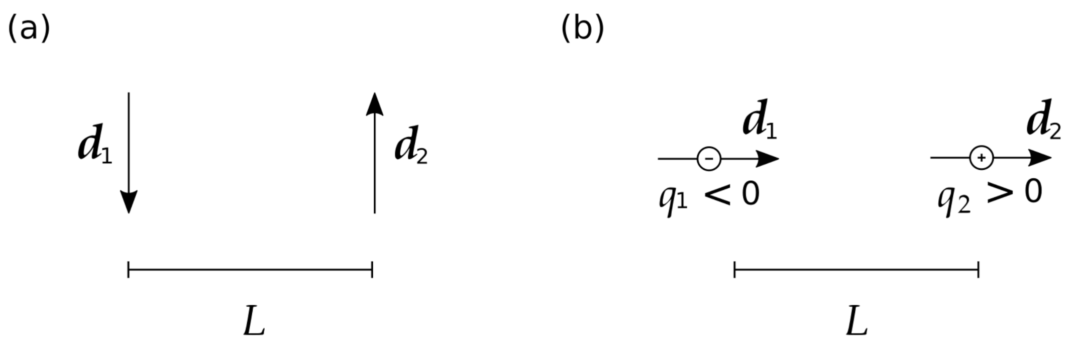
An interesting feature of these results is that, for positive polarizabilities, the monopole-dipole interaction weakens the attraction between the spheres. A simple physical picture can explain this. In order to minimize the energy, the correlations between the fluctuating dipoles favor dipole orientations that lead to attraction. If the dipoles are perpendicular to the line connecting the spheres, then the dipoles should be anti-parallel, as indicated in Figure 4a.

From Equation (48), we see that the charge induced by each dipole is proportional to the electric potential they generate at the center of the other sphere. A point dipole $\mathit{d}$ produces a potential at a point P that is proportional to $\mathit{d}·\widehat{\mathit{r}}$, where $\widehat{\mathit{r}}$ is the unit vector corresponding to the position $\mathit{r}$ of the point P. Therefore, when the dipoles are perpendicular to the line connecting the spheres, they do not induce any charge. On the other hand, when the dipoles are parallel to the line connecting the spheres, the energetically favored configuration is the one where the dipoles are parallel to each other. This orientation is the one that yields the largest induced monopole induced on the spheres for a fixed distance, since the charge is proportional to the potential. As illustrated in Figure 4b, in this configuration, we induce charges of opposite sign in each sphere, thus yielding an attractive monopole-monopole correlation, as expected. However, the interaction of the charge induced in one sphere with the dipole induced on the other sphere is repulsive. Even though we should average over all orientations, this argument shows that situations close to the one depicted in Figure 4b are the dominant ones for effects associated with the monopole fluctuations. Hence, the monopole-dipole interaction is repulsive and, thus, weakens the overall attraction between the spheres. On the other hand, if the spheres’ polarizability is negative (that is, if their permittivities are smaller that of the electrolyte in between), the argument is reversed and the monopole-dipole interaction enhances the spheres’ attraction. Since the potential generated by each dipole changes sign in comparison to the case of positive polarizability, the signs of the induced charges must be reversed in comparison to Figure 4b.

There is, however, yet more to be uncovered. By substituting the expression for ${\kappa }_D$ (4) in the first term of (46), we get

$$F_{\mathrm{mon}-\mathrm{mon}}=-\left(c_0{q}^2\frac{8\pi }{3}{R}_1^3\right)\left(c_0{q}^2\frac{8\pi }{3}{R}_2^3\right)\frac{e^{-2{\kappa }_{D}L}}{32{\pi }^2{ϵ}_3^2\left(k_{B}T\right)L^2},$$

(63)

which has precisely the form of the Kirkwood-Shumaker interaction between two proteins undergoing charge fluctuations [63,64,65] (accounting for the difference in systems of units employed) if one identifies

$$\frac{8\pi }{3}{c}_0{q}^2{R}_s^3=\langle \mathrm{\Delta }{Q}_s^2\rangle s=1,2,$$

(64)

where $\mathrm{\Delta }{Q}_s$ is the fluctuation of charge at the s-th particle. This result is interesting because it provides a nice analogy between a more familiar example of monopole fluctuations—the exchange of protons between proteins and the surrounding solution—and our setup, where such intermittent monopoles arise due to the fluctuations of the electric potential and the “room” created by the excluded volume. We can verify the relation (64) by noting that the average energy associated with the monopole of particle s is $\langle \mathrm{\Delta }{Q}_s^2\rangle /2C_s=k_{B}T/2$ by virtue of the equipartition theorem. Combining this result with Equations (4) and (49), we obtain a third derivation of the expression (64) for the monopole fluctuations.

As an additional remark, we note that Equation (63) is reminiscent of the orientation/Keesom interaction between dipoles [52]

$${\mathcal{F}}_{\mathrm{Keesom}}\sim -\frac{\langle {\mathbf{p}}_1^2\rangle \langle {\mathbf{p}}_2^2\rangle }{\left(k_{B}T\right)L^6},$$

(65)

where $\langle {\mathbf{p}}_s^2\rangle$ is the second moment of the s-th dipole. This observation is noteworthy because it unveils a pattern that should always be present when fluctuating quantities of vanishing (linear) mean interact in such a way as to have their interaction energy much smaller than $k_{B}T$. For the sake of illustration, let us say that we have two fluctuating particles that have an instantaneous interaction energy of $U_{12}$. By averaging over the appropriate ensemble, we get

$$\begin{array}{c}\hfill {\mathcal{F}}_{12}=-k_{B}Tlog\langle e^{-U_{12}/k_{B}T}\rangle \approx -k_{B}Tlog\left[1-\frac{\langle U_{12}\rangle }{k_{B}T}+\frac{\langle U_{12}^2\rangle }{2{\left(k_{B}T\right)}^2}\right]\approx -\frac{\langle U_{12}^2\rangle }{2k_{B}T},\end{array}$$

(66)

where we used the assumptions that $\langle U_{12}\rangle =0$ and $U_{12}\ll k_{B}T$. Even though Keesom considered randomly oriented permanent dipoles in contrast to our situation of no permanent multipoles, it can now be easily understood why expressions (65) and (63) are so similar. $U_{12}$ just needs to be replaced by either the monopole-monopole interaction ($q_1{q}_2/L$) or dipole-dipole interaction (${\mathbf{p}}_1·{\mathbf{p}}_2/L^3$).

Last but not least, we should point out that, due to the presence of a monopolar term in (46), the small radii limit of ${\mathcal{F}}_{\mathrm{cas}}^0$ has a contribution that is completely independent of the material properties of the interacting objects. In other words: provided that the distance between the objects is not so large as to have the $n=0$ term screened by the ions, our results indicate that a significant contribution to the dispersive force between two small particles of any kind is solely determined by their size and the ionic concentration in the electrolyte, which could lead to interesting experimental prospects.

3.5. Very Large Spheres and Comparison with PFA

We now discuss the opposite limit of large radii and compare our results with the widely employed proximity force approximation (PFA), also known as Derjaguin approximation [88], which effectively describes the interacting (smooth) surfaces by tiny contiguous planes [89]. The PFA holds as a limit when the spheres’ radii are much larger than the surface separation [73], i.e.,

$${\displaystyle \frac{a}{R_s}}\ll 1,s=1,2.$$

(67)

The free energy between two spheres in the PFA is given by

$${\mathcal{F}}_{\mathrm{PFA}}\left(a\right)=\frac{2\pi R_{\mathrm{eff}}}{A}{\int }_a^{\infty }\mathrm{d}l{\mathcal{F}}_{\mathrm{pl}-\mathrm{pl}}\left(l\right),$$

(68)

where $R_{\mathrm{eff}}=R_1{R}_2/(R_1+R_2)$, and ${\mathcal{F}}_{\mathrm{pl}-\mathrm{pl}}\left(a\right)$ is the interaction energy between two parallel planar surfaces [57].

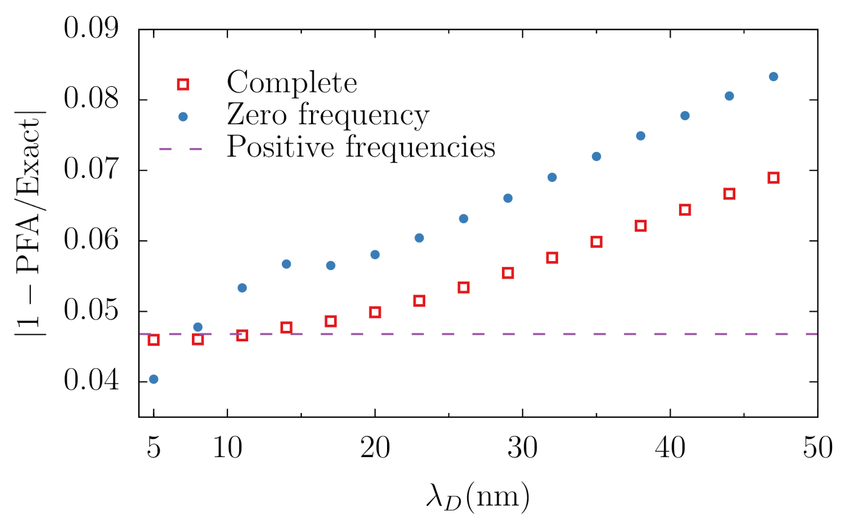
In Figure 5, we plot the relative discrepancy between the PFA and the exact result as a function of the Debye length ${\lambda }_D$ for two PS spheres with $R_1=R_2=1\mathsf{\mu }\mathrm{m}$ separated by a distance $a=20\mathrm{nm}.$ More specifically, the red squares represent the relative discrepancy between the exact and PFA free energies

$$\delta =\frac{{\mathcal{F}}_{\mathrm{cas}}-{\mathcal{F}}_{\mathrm{PFA}}}{{\mathcal{F}}_{\mathrm{cas}}},$$

(69)

while the blue dots show the zeroth frequency discrepancy ${\delta }_0$, for which only the zeroth Matsubara contributions are taken in (69). A similar comparison was carried out in Ref. [59] in the cases of complete screening (${\lambda }_D\to 0$) and no screening (${\lambda }_D\to \infty$). The former corresponds to the value $\delta =0.047$ indicated as a dashed line. We see a monotonic growth of $\delta$ for the total free energy as the screening decreases, which we attribute to (i) an increase of the relative contribution of the zeroth Matsubara frequency, for which the PFA is generally less accurate, e.g., ${\delta }_0=0.34$ in the absence of screening for the parameters in Figure 5, and (ii) to the overall increase of ${\delta }_0$ as function of ${\lambda }_D.$ The latter behavior can be expected because PFA assumes that the interaction between the “effective plates” decays sufficiently rapidly [89], and the screening cuts off the interaction exponentially. Therefore, the lower is ${\lambda }_D$ (and the stronger is the screening), the lower is the discrepancy.

For the variation of ${\delta }_0$ with decreasing Debye length, Figure 5 shows a sudden breaking of the monotonic trend at ${\lambda }_D\approx a=20$ nm, indicating a nontrivial interplay between the two scales, and then a sharp drop as the Debye length gets below 15 nm. The latter may be understood along the same lines of the previous paragraph, as the interaction range gets substantially smaller than the separation gap and then the PFA is expected to work increasingly better for the zeroth frequency contribution [89]. That a different behavior is displayed by the red squares for the discrepancy of the total free energy is not surprising: the contribution of the zeroth frequency term to the total free energy becomes quite small at that range—for instance, for a Debye length of 8 nm, the zeroth frequency contribution is $2\%$ of the total force—so the variation with ${\lambda }_D$ becomes negligible.

4. Conclusions

We have considered the Casimir interaction between two dielectric spherical particles immersed in aqueous solution. As the distance rises, screening by ions in solution increasingly suppresses the Matsubara zero-frequency thermal contribution, which would otherwise be the dominant contribution at distances ≳0.1 μm. We have derived a general representation for the zero-frequency contribution by analyzing multipolar fluctuations as governed by the linear Poisson-Boltzmann equation in the electrolyte region.

In the limit of very small spheres, we have re-obtained the screened interaction between fluctuating dipoles of Ref. [56]. However, two additional contributions turn out to also be of order ${\left(R_1{R}_2\right)}^3.$ They arise from monopole fluctuations associated to the volume of electrolyte solution excluded by each sphere. The monopole-monopole term depends on the volume of the particles only and not on their dielectric constants. The monopole-dipole contribution tends to reduce the attraction when the particles’ dielectric constant is larger than the external one. As a verification and for the sake of physical insight, we have developed an alternative derivation based on the cross correlations between monopole and dipole moments.

When considering the opposite limit of large spheres, we were able make contact with the known result for parallel planar surfaces [55,56,57] with the help of the proximity force (Derjaguin) approximation [88,89]. We have provided a detailed comparison between such widely-employed approximation and our multipolar results obtained from exact solutions of the linear Poisson-Boltzmann equation for the sphere-sphere geometry. As expected, for a given geometric aspect ratio $a/R_s,$ the approximation becomes increasingly accurate as screening is enhanced by adding salt to the solution.

The electrostatic fluctuational approach we have followed should hold for moderately short distances $a\lesssim {\lambda }_D$ and allows one to recover the ion-free case in the limit ${\lambda }_D\to \infty .$ For very short distances, one could expect deviations as the mean-field approximation behind the linear Poisson-Boltzmann equation breaks down [90]. However, in this case, the zero-frequency contribution is generally less important, and then so is the ionic screening of the Casimir interaction. On the other hand, for longer distances, $a>{\lambda }_D,$ the Casimir effect in electrolyte media can be cast in terms of the scattering approach by taking into account the spatially non-local response of the movable ions in the bulk approximation [54]. For parallel planar surfaces, the resulting zero-frequency contribution contains not only the result obtained from the electrostatic fluctuational approach but also an additional term arising from transverse magnetic modes [58]. A similar result is expected for the spherical geometry, and a derivation is currently under way. A more general theory, valid for arbitrary values of $a/{\lambda }_D$ and describing the crossover region $a\sim {\lambda }_D$, will require an implementation of the scattering approach beyond the bulk approximation for the non-local response of the electrolyte solution, possibly along the lines of Ref. [53].

References

- Casimir, H.B.G. On the attraction between two perfectly conducting plates. Proc. Kon. Ned. Akad. Wetensch. 1948, 51, 793. [Google Scholar]
- Lifshitz, E. The theory of molecular attractive forces between solid bodies. J. Exp. Theor. Phys. USSR 1955, 2, 73. [Google Scholar]
- Dalvit, D.; Milonni, P.; Roberts, D.; Da Rosa, F. Casimir Physics; Springer: Berlin/Heidelberg, Germany, 2011; Volume 834. [Google Scholar]
- Woods, L.M.; Dalvit, D.A.R.; Tkatchenko, A.; Rodriguez-Lopez, P.; Rodriguez, A.W.; Podgornik, R. Materials perspective on Casimir and van der Waals interactions. Rev. Mod. Phys. 2016, 88, 045003. [Google Scholar] [CrossRef]
- Bordag, M.; Klimchitskaya, G.L.; Mohideen, U.; Mostepanenko, V.M. Advances in the Casimir Effect; OUP Oxford: New York, NY, USA, 2009; Volume 145. [Google Scholar]
- Buhmann, S.Y. Dispersion Forces I: Macroscopic Quantum Electrodynamics and Ground-State Casimir, Casimir–Polder and van der Waals Forces; Springer: Berlin/Heidelberg, Germany, 2012; Volume 247. [Google Scholar]
- Rodriguez, A.; Ibanescu, M.; Iannuzzi, D.; Joannopoulos, J.D.; Johnson, S.G. Virtual photons in imaginary time: Computing exact Casimir forces via standard numerical electromagnetism techniques. Phys. Rev. A 2007, 76, 032106. [Google Scholar] [CrossRef] [Green Version]
- Reid, M.T.H.; White, J.; Johnson, S.G. Fluctuating surface currents: An algorithm for efficient prediction of Casimir interactions among arbitrary materials in arbitrary geometries. Phys. Rev. A 2013, 88, 022514. [Google Scholar] [CrossRef] [Green Version]
- Hartmann, M.; Ingold, G.L.; Maia Neto, P.A. Plasma versus Drude Modeling of the Casimir Force: Beyond the Proximity Force Approximation. Phys. Rev. Lett. 2017, 119, 043901. [Google Scholar] [CrossRef]
- Hartmann, M.; Ingold, G.L.; Neto, P.A.M. Advancing numerics for the Casimir effect to experimentally relevant aspect ratios. Phys. Scr. 2018, 93, 114003. [Google Scholar] [CrossRef] [Green Version]
- Dzyaloshinskii, I.E.; Lifshitz, E.M.; Pitaevskii, L.P. The General Theory of Van der Waals Forces. Adv. Phys. 1961, 10, 165. [Google Scholar] [CrossRef]
- Renne, M.J. Microscopic theory of retarded Van der Waals forces between macroscopic dielectric bodies. Physica 1971, 56, 125. [Google Scholar] [CrossRef] [Green Version]
- Barash, Y.S.; Ginzburg, V.L. Electromagnetic fluctuations in matter and molecular (Van-der-Waals) forces between them. Sov. Phys. Uspekhi 1975, 18, 305. [Google Scholar] [CrossRef]
- Schwinger, J.; DeRaad, L.L., Jr.; Milton, K.A. Casimir effect in dielectrics. Ann. Phys. (N. Y.) 1978, 115, 1–23. [Google Scholar] [CrossRef]
- Lambrecht, A.; Maia Neto, P.A.; Reynaud, S. The Casimir effect within scattering theory. New J. Phys. 2006, 8, 243. [Google Scholar] [CrossRef] [Green Version]
- Rahi, S.J.; Emig, T.; Graham, N.; Jaffe, R.L.; Kardar, M. Scattering theory approach to electrodynamic Casimir forces. Phys. Rev. D 2009, 80, 085021. [Google Scholar] [CrossRef] [Green Version]
- Bulgac, A.; Magierski, P.; Wirzba, A. Scalar Casimir effect between Dirichlet spheres or a plate and a sphere. Phys. Rev. D 2006, 73, 025007. [Google Scholar] [CrossRef] [Green Version]
- Emig, T.; Graham, N.; Jaffe, R.L.; Kardar, M. Casimir Forces between Arbitrary Compact Objects. Phys. Rev. Lett. 2007, 99, 170403. [Google Scholar] [CrossRef] [PubMed] [Green Version]
- Canaguier-Durand, A.; Maia Neto, P.A.; Cavero-Pelaez, I.; Lambrecht, A.; Reynaud, S. Casimir Interaction between Plane and Spherical Metallic Surfaces. Phys. Rev. Lett. 2009, 102, 230404. [Google Scholar] [CrossRef]
- Rodriguez-Lopez, P. Casimir energy and entropy in the sphere-sphere geometry. Phys. Rev. B 2011, 84, 075431. [Google Scholar] [CrossRef] [Green Version]
- Bordag, M. Casimir effect for a sphere and a cylinder in front of a plane and corrections to the proximity force theorem. Phys. Rev. D 2006, 73, 125018. [Google Scholar] [CrossRef] [Green Version]
- Gies, H.; Klingmüller, K. Casimir Effect for Curved Geometries: Proximity-Force-Approximation Validity Limits. Phys. Rev. Lett. 2006, 96, 220401. [Google Scholar] [CrossRef] [Green Version]
- Rodrigues, R.B.; Maia Neto, P.A.; Lambrecht, A.; Reynaud, S. Vacuum-induced torque between corrugated metallic plates. Europhys. Lett. 2006, 76, 822. [Google Scholar] [CrossRef]
- Rodrigues, R.B.; Maia Neto, P.A.; Lambrecht, A.; Reynaud, S. Lateral Casimir force beyond the proximity force approximation: A nontrivial interplay between geometry and quantum vacuum. Phys. Rev. A 2007, 75, 062108. [Google Scholar] [CrossRef] [Green Version]
- Lambrecht, A.; Marachevsky, V.N. Casimir Interaction of Dielectric Gratings. Phys. Rev. Lett. 2008, 101, 160403. [Google Scholar] [CrossRef] [Green Version]
- Lussange, J.; Guérout, R.; Lambrecht, A. Casimir energy between nanostructured gratings of arbitrary periodic profile. Phys. Rev. A 2012, 86, 062502. [Google Scholar] [CrossRef] [Green Version]
- Messina, R.; Maia Neto, P.A.; Guizal, B.; Antezza, M. Casimir interaction between a sphere and a grating. Phys. Rev. A 2015, 92, 062504. [Google Scholar] [CrossRef] [Green Version]
- Ran, Z.; Ya-Ping, Y. Repulsive and Restoring Casimir Forces Based on Magneto-Optical Effect. Chin. Phys. Lett. 2011, 28, 054201. [Google Scholar] [CrossRef]
- Cysne, T.; Kort-Kamp, W.J.M.; Oliver, D.; Pinheiro, F.A.; Rosa, F.S.S.; Farina, C. Tuning the Casimir-Polder interaction via magneto-optical effects in graphene. Phys. Rev. A 2014, 90, 052511. [Google Scholar] [CrossRef] [Green Version]
- Emelianova, N.; Fialkovsky, I.V.; Khusnutdinov, N. Casimir effect for biaxial anisotropic plates with surface conductivity. Mod. Phys. Lett. A 2020, 35, 2040012. [Google Scholar] [CrossRef] [Green Version]
- Barton, G. Some surface effects in the hydrodynamic model of metals. Rep. Prog. Phys. 1979, 42, 963. [Google Scholar] [CrossRef]
- Mochán, W.L.; Villarreal, C.; Esquivel-Sirvent, R. On Casimir forces for media with arbitrary dielectric properties. Rev. Mex. Fís. 2002, 48, 339–342. [Google Scholar]
- Esquivel-Sirvent, R.; Villarreal, C.; Mochán, W.L.; Contreras-Reyes, A.M.; Svetovoy, V.B. Spatial dispersion in Casimir forces: A brief review. J. Phys. A Math. Gen. 2006, 39, 6323. [Google Scholar] [CrossRef]
- Svetovoy, V.B. Application of the Lifshitz Theory to Poor Conductors. Phys. Rev. Lett. 2008, 101, 163603. [Google Scholar] [CrossRef] [PubMed] [Green Version]
- Pitaevskii, L.P. Thermal Lifshitz Force between an Atom and a Conductor with a Small Density of Carriers. Phys. Rev. Lett. 2008, 101, 163202. [Google Scholar] [CrossRef] [PubMed] [Green Version]
- Parsegian, V.A.; Weiss, G.H. Dielectric Anisotropy and the van der Waals Interaction between Bulk Media. J. Adhes. 1972, 3, 259–267. [Google Scholar] [CrossRef]
- Barash, Y.S. Moment of van der Waals forces between anisotropic bodies. Radiophys. Quantum Electron. 1978, 21, 1138–1143. [Google Scholar] [CrossRef]
- Rosa, F.S.S.; Dalvit, D.A.R.; Milonni, P.W. Casimir interactions for anisotropic magnetodielectric metamaterials. Phys. Rev. A 2008, 78, 032117. [Google Scholar] [CrossRef] [Green Version]
- Bimonte, G. Casimir effect in a superconducting cavity and the thermal controversy. Phys. Rev. A 2008, 78, 062101. [Google Scholar] [CrossRef] [Green Version]
- Inui, N. Temperature dependence of the Casimir force between a superconductor and a magnetodielectric. Phys. Rev. A 2012, 86, 022520. [Google Scholar] [CrossRef]
- Torricelli, G.; van Zwol, P.J.; Shpak, O.; Binns, C.; Palasantzas, G.; Kooi, B.J.; Svetovoy, V.B.; Wuttig, M. Switching Casimir forces with phase-change materials. Phys. Rev. A 2010, 82, 010101. [Google Scholar] [CrossRef] [Green Version]
- Rodriguez-Lopez, P.; Kort-Kamp, W.J.; Dalvit, D.A.; Woods, L.M. Casimir force phase transitions in the graphene family. Nature Commun. 2017, 8, 1–9. [Google Scholar] [CrossRef] [Green Version]
- Tabor, D.; Winterton, R. Surface forces: Direct measurement of normal and retarded van der Waals forces. Nature 1968, 219, 1120–1121. [Google Scholar] [CrossRef]
- Sabisky, E.S.; Anderson, C.H. Verification of the Lifshitz Theory of the van der Waals Potential Using Liquid-Helium films. Phys. Rev. A 1973, 7, 790. [Google Scholar] [CrossRef]
- Lamoreaux, S.K. Demonstration of the Casimir Force in the 0.6 to 6 μm Range. Phys. Rev. Lett. 1997, 78, 5. [Google Scholar] [CrossRef] [Green Version]
- Mohideen, U.; Roy, A. Precision Measurement of the Casimir Force from 0.1 to 0.9 μm. Phys. Rev. Lett. 1998, 81, 4549. [Google Scholar] [CrossRef] [Green Version]
- Decca, R.S.; López, D.; Fischbach, E.; Klimchitskaya, G.L.; Krause, D.E.; Mostepanenko, V.M. Precise comparison of theory and new experiment for the Casimir force leads to stronger constraints on thermal quantum effects and long-range interactions. Ann. Phys. (N. Y.) 2005, 318, 37–80. [Google Scholar] [CrossRef] [Green Version]
- Munday, J.N.; Capasso, F.; Parsegian, V.A. Measured long-range repulsive Casimir–Lifshitz forces. Nature 2009, 457, 170–173. [Google Scholar] [CrossRef]
- van Zwol, P.J.; Palasantzas, G.; De Hosson, J.T.M. Influence of dielectric properties on van der Waals/Casimir forces in solid-liquid systems. Phys. Rev. B 2009, 79, 195428. [Google Scholar] [CrossRef] [Green Version]
- Tang, L.; Wang, M.; Ng, C.; Nikolic, M.; Chan, C.T.; Rodriguez, A.W.; Chan, H.B. Measurement of non-monotonic Casimir forces between silicon nanostructures. Nat. Photonics 2017, 11, 97–101. [Google Scholar] [CrossRef] [Green Version]
- Butt, H.J.; Kappl, M. Surface and Interfacial Forces; Wiley Online Library: Weinheim, Germany, 2010. [Google Scholar]
- Israelachvili, J.N. Intermolecular and Surface Forces; Academic Press: Burlington, MA, USA, 2015. [Google Scholar]
- Gorelkin, V.N.; Smilga, V.P. Calculation of Intermolecular Interaction Forces Between Bodies Separated by a Film of a Strong Electrolyte Solution. Sov. Phys. JETP 1973, 36, 761. [Google Scholar]
- Davies, B.; Ninham, B.W. Van der Waals Forces in Electrolytes. J. Chem. Phys. 1972, 56, 5797–5801. [Google Scholar] [CrossRef]
- Mitchell, D.J.; Richmond, P. A General Formalism for the Calculation of Free Energies of Inhomogeneous Dielectric and Electrolyte System. J. Colloid Interface Sci. 1974, 46, 118–127. [Google Scholar] [CrossRef]
- Mahanty, J.; Ninham, B.W. Dispersion Forces; Academic Press: New York, NY, USA, 1976; Volume 1. [Google Scholar]
- Parsegian, V.A. Van der Waals forces: A Handbook for Biologists, Chemists, Engineers, and Physicists; Cambridge University Press: New York, NY, USA, 2005. [Google Scholar]
- Neto, P.A.M.; Rosa, F.S.S.; Pires, L.B.; Moraes, A.; Canaguier-Durand, A.; Guérout, R.; Lambrecht, A.; Reynaud, S. Scattering theory of the screened Casimir interaction in electrolytes. Eur. Phys. J. D 2019, 73, 178. [Google Scholar] [CrossRef] [Green Version]
- Spreng, B.; Maia Neto, P.A.; Ingold, G.L. Plane-wave approach to the exact van der Waals interaction between colloid particles. J. Chem. Phys. 2020, 153, 024115. [Google Scholar] [CrossRef] [PubMed]
- Ninham, B.W.; Nostro, P.L. Molecular Forces and Self Assembly: In Colloid, Nano Sciences and Biology; Cambridge University Press: New York, NY, USA, 2010. [Google Scholar]
- Carnie, S.L.; Chan, D.Y.C.; Gunning, J.S. Electrical Double Layer Interaction between Dissimilar Spherical Colloidal Particles and between a Sphere and a Plate: The Linearized Poisson-Boltzmann Theory. Langmuir 1994, 10, 2993–3009. [Google Scholar] [CrossRef]
- Langbein, D. Theory of van der Waals Attraction. In Springer Tracts in Modern Physics; Springer: Berlin/Heidelberg, Germany, 1974; pp. 1–139. [Google Scholar]
- Kirkwood, J.G.; Shumaker, J.B. Forces between Protein Molecules in Solution Arising from Fluctuations in Proton Charge and Configuration. Proc. Natl. Acad. Sci. USA 1952, 38, 863. [Google Scholar] [CrossRef] [Green Version]
- Adžić, N.; Podgornik, R. Field-theoretic description of charge regulation interaction. Eur. Phys. J. E 2014, 37, 49. [Google Scholar] [CrossRef] [PubMed] [Green Version]
- Adžić, N.; Podgornik, R. Charge regulation in ionic solutions: Thermal fluctuations and Kirkwood-Schumaker interactions. Phys. Rev. E 2015, 91, 022715. [Google Scholar] [CrossRef] [Green Version]
- Kampen, N.G.V.; Nijboer, B.R.A.; Schram, K. On the Macroscopic Theory of Van der Waals Forces. Phys. Lett. 1968, 26A, 307–308. [Google Scholar] [CrossRef] [Green Version]
- Milonni, P.W. The Quantum Vacuum: An Introduction to Quantum Electrodynamics; Academic Press: San Diego, CA, USA, 2013. [Google Scholar]
- Tomaš, M.S. Casimir force in absorbing multilayers. Phys. Rev. A 2002, 66, 052103. [Google Scholar] [CrossRef] [Green Version]
- Intravaia, F.; Behunin, R. Casimir effect as a sum over modes in dissipative systems. Phys. Rev. A 2012, 86, 062517. [Google Scholar] [CrossRef] [Green Version]
- Pires, L.B.; Ether, D.S.; Spreng, B.; Araújo, G.R.S.; Decca, R.S.; Dutra, R.S.; Borges, M.; Rosa, F.S.S.; Ingold, G.L.; Moura, M.J.B.; et al. Probing the screening of the Casimir interaction with optical tweezers. arXiv 2021, arXiv:2104.00157. [Google Scholar]
- NIST Digital Library of Mathematical Functions. Available online: http://dlmf.nist.gov/ (accessed on 15 May 2021).
- Umrath, S.; Hartmann, M.; Ingold, G.L.; Maia Neto, P.A. Disentangling geometric and dissipative origins of negative Casimir entropies. Phys. Rev. E 2015, 92, 042125. [Google Scholar] [CrossRef] [PubMed]
- Spreng, B.; Hartmann, M.; Henning, V.; Maia Neto, P.A.; Ingold, G.L. Proximity force approximation and specular reflection: Application of the WKB limit of Mie scattering to the Casimir effect. Phys. Rev. A 2018, 97, 062504. [Google Scholar] [CrossRef]
- Henning, V.; Spreng, B.; Hartmann, M.; Ingold, G.L.; Maia Neto, P.A. The role of diffraction in the Casimir effect beyond the proximity force approximation. J. Opt. Soc. Am. B 2019, 36, C77–C87. [Google Scholar] [CrossRef] [Green Version]
- Bohren, C.F.; Huffman, D.R. Absorption and Scattering of Light by Small Particles; John Wiley & Sons: Weinheim, Germany, 2008. [Google Scholar]
- Bornemann, F. On the numerical evaluation of Fredholm determinants. Math. Comp. 2010, 79, 871–915. [Google Scholar] [CrossRef]
- Boyd, J.P. Exponentially convergent Fourier-Chebshev quadrature schemes on bounded and infinite intervals. J. Sci. Comput. 1987, 2, 99–109. [Google Scholar] [CrossRef] [Green Version]
- Canaguier-Durand, A.; Guérout, R.; Neto, P.A.M.; Lambrecht, A.; Reynaud, S. The Casimir effect in the sphere-plane geometry. Int. J. Mod. Phys. Conf. Ser. 2012, 14, 250–259. [Google Scholar] [CrossRef] [Green Version]
- Umrath, S. Der Casimir-Effekt in der Kugel-Kugel-Geometrie: Theorie und Anwendung auf das Experiment. Ph.D. Thesis, Universität Augsburg, Augsburg, Germany, 2016. Available online: https://opus.bibliothek.uni-augsburg.de/opus4/3763 (accessed on 16 May 2021).
- Pikhitsa, P.V.; Tsargorodskaya, A.B.; Kontush, S.M. A Phenomenon of the Change in Particle Drift Velocity Direction in High-Field Electrophoresis. J. Colloid Interface Sci. 2000, 230, 334–339. [Google Scholar] [CrossRef]
- Hansen, P.M.; Dreyer, J.K.; Ferkinghoff-Borg, J.; Oddershede, L. Novel optical and statistical methods reveal colloid–wall interactions inconsistent with DLVO and Lifshitz theories. J. Colloid Interface Sci. 2005, 287, 561–571. [Google Scholar] [CrossRef]
- Schäffer, E.; Nørrelykke, S.F.; Howard, J. Surface Forces and Drag Coefficients of Microspheres near a Plane Surface Measured with Optical Tweezers. Langmuir 2007, 23, 3654–3665. [Google Scholar] [CrossRef]
- Gutsche, C.; Keyser, U.F.; Kegler, K.; Kremer, F.; Linse, P. Forces between single pairs of charged colloids in aqueous salt solutions. Phys. Rev. E 2007, 76, 031403. [Google Scholar] [CrossRef] [Green Version]
- Ether, D.S., Jr.; Pires, L.B.; Umrath, S.; Martinez, D.; Ayala, Y.; Pontes, B.; de Sousa Araújo, G.R.; Frases, S.; Ingold, G.L.; Rosa, F.S.S.; et al. Probing the Casimir force with optical tweezers. EPL (Europhys. Lett.) 2015, 112, 44001. [Google Scholar] [CrossRef] [Green Version]
- Kundu, A.; Paul, S.; Banerjee, S.; Banerjee, A. Measurement of Van der Waals force using oscillating optical tweezers. Appl. Phys. Lett. 2019, 115, 123701. [Google Scholar] [CrossRef]
- Griffiths, D.J. Introduction to Electrodynamics; Prentice Hall: Englewood Cliffs, NJ, USA, 1999. [Google Scholar]
- Pitombo, R.S.; Vasconcellos, M.; Farina, C.; de Melo e Souza, R. Source method for the evaluation of multipole fields. EJP (Eur. J. Phys.) 2021, 42, 025202. [Google Scholar]
- Derjaguin, B. Untersuchungen über die Reibung und Adhäsion, IV. Kolloid-Zeitschrift 1934, 69, 155–164. [Google Scholar] [CrossRef]
- Błocki, J.; Randrup, J.; Świa̧tecki, W.J.; Tsang, C.F. Proximity forces. Ann. Phys. (N. Y.) 1977, 105, 427–462. [Google Scholar] [CrossRef]
- Ben-Yaakov, D.; Andelman, D.; Harries, D.; Podgornik, R. Scattering theory of the screened Casimir interaction in electrolytes. J. Phys. Condens. Matter 2009, 21, 424106. [Google Scholar] [CrossRef] [PubMed]
Figure 1.
Description of the geometry with two solid spheres of radii and separated by a center-to-center distance L along the z-axis. We also indicate the surface-to-surface distance . A generic point can be described using either sphere center: () is a vector from the center of the sphere 1 (2) to the point.
Figure 2.
Variation with the surface-to-surface distance of the (a) Casimir free energy, (b) Casimir force, (c) relative zero frequency contribution to the free energy, and (d) relative zero frequency contribution to the force. We consider two PS spheres of radius .
Figure 3.
Zero-frequency contribution to the Casimir energy for two silica spheres of radius R as a function of for a fixed and different Debye lengths: numerical (solid) and small-sphere approximation (46) (dashed).
Figure 4.
Attractive electrostatic interaction between two fluctuating dipoles in an electrolyte solution for two configurations: (a) Dipoles perpendicular to the line connecting them and (b) Dipoles parallel to the line connecting them. In situation (a), the electrostatic potential generated by each dipole does not induce a charge, while, in situation (b), it does, with the signs indicated in the figure.
Figure 5.
Relative discrepancy between the PFA and the exact result as a function of the Debye length for the total free energy (red squares) and the zero-frequency contribution (blue dots). The horizontal dashed line indicates the discrepancy when considering positive frequencies only, which do not depend on We consider two PS spheres of radius 1 μm separated by a distance of 20 nm.
Publisher’s Note: MDPI stays neutral with regard to jurisdictional claims in published maps and institutional affiliations. |
© 2021 by the authors. Licensee MDPI, Basel, Switzerland. This article is an open access article distributed under the terms and conditions of the Creative Commons Attribution (CC BY) license (https://creativecommons.org/licenses/by/4.0/).
Share and Cite
MDPI and ACS Style
Nunes, R.O.; Spreng, B.; de Melo e Souza, R.; Ingold, G.-L.; Maia Neto, P.A.; Rosa, F.S.S. The Casimir Interaction between Spheres Immersed in Electrolytes. Universe 2021, 7, 156. https://0-doi-org.brum.beds.ac.uk/10.3390/universe7050156
AMA Style
Nunes RO, Spreng B, de Melo e Souza R, Ingold G-L, Maia Neto PA, Rosa FSS. The Casimir Interaction between Spheres Immersed in Electrolytes. Universe. 2021; 7(5):156. https://0-doi-org.brum.beds.ac.uk/10.3390/universe7050156
Chicago/Turabian StyleNunes, Renan O., Benjamin Spreng, Reinaldo de Melo e Souza, Gert-Ludwig Ingold, Paulo A. Maia Neto, and Felipe S. S. Rosa. 2021. "The Casimir Interaction between Spheres Immersed in Electrolytes" Universe 7, no. 5: 156. https://0-doi-org.brum.beds.ac.uk/10.3390/universe7050156
Note that from the first issue of 2016, this journal uses article numbers instead of page numbers. See further details here.