
Epicyclic Oscillations around Simpson–Visser Regular Black Holes and Wormholes

Research Centre of Theoretical Physics and Astrophysics, Institute of Physics, Silesian University in Opava, Bezručovo Nám. 13, CZ-746 01 Opava, Czech Republic
*
Author to whom correspondence should be addressed.
Universe 2021, 7(8), 279; https://0-doi-org.brum.beds.ac.uk/10.3390/universe7080279
Submission received: 29 June 2021
/
Revised: 21 July 2021
/
Accepted: 28 July 2021
/
Published: 1 August 2021
(This article belongs to the Special Issue Recent Advances in Wormhole Physics)
Abstract
:We study epicyclic oscillatory motion along circular geodesics of the Simpson–Visser meta-geometry describing in a unique way regular black-bounce black holes and reflection-symmetric wormholes by using a length parameter l. We give the frequencies of the orbital and epicyclic motion in a Keplerian disc with inner edge at the innermost circular geodesic located above the black hole outer horizon or on the our side of the wormhole. We use these frequencies in the epicyclic resonance version of the so-called geodesic models of high-frequency quasi-periodic oscillations (HF QPOs) observed in microquasars and around supermassive black holes in active galactic nuclei to test the ability of this meta-geometry to improve the fitting of HF QPOs observational data from the surrounding of supermassive black holes. We demonstrate that this is really possible for wormholes with sufficiently high length parameter l.
1. Introduction
Simpson and Visser introduced a very simple theoretically attractive spherically symmetric model of meta-geometry, coming from the Schwarzschild geometry and enabling a unique description of regular black holes and wormholes by smooth interpolation between these two possibilities using a length-scale parameter l responsible for regularization of the central singularity and potentially reflecting in a maximally simple way the possible influence of quantum gravity effects; its rotation version has recently also been presented [1,2]. The Simpson–Visser wormhole is traversable in the same way as the standard Morris–Thorne wormhole solutions [3,4], thus representing a spacetime tunnel connecting distant parts of the Universe (or different universes) that enables the transfer of massive objects. The Simpson–Visser regular black hole demonstrates a black bounce that occurs behind the black hole horizon, being similar to the idea of the black universe [5].
The simple case of the reflection-symmetric traversable wormholes was introduced by Visser [6,7] where two Schwarzschild spacetimes are connected by a spherical shell of extraordinary matter with negative energy density violating the weak energy condition, located at the junction and guaranteeing correctness of the Einstein gravitational equations for the stable traversable wormholes [8]. In the high-dimensional general relativity [9], or some alternative gravity theories [10], such extraordinary form of the stress–energy tensor can be avoided in the wormhole solutions. Moreover, the traversable wormholes constructed without extraordinary forms of matter or alternative gravity are possible for fermions giving a negative Casimir energy [11]—in the Einstein–Dirac theory or the Einstein–Maxwell–Dirac theory [12,13].
Extraordinary recent results of the radio-interferometry observational systems, namely of the Event Horizon Telescope (ETH) and GRAVITY [14], give insight into the innermost region of accretion discs orbiting supermassive black holes such as SgrA* in the Galaxy center, or those in the center of active nucleus of the M87 galaxy. The accreting matter reflecting the shadow of the assumed central rotating Kerr black hole was observed in the SgrA* by GRAVITY, and in the central region of M87 in [15] by EHT. These observations of the assumed close vicinity of the black hole horizon inspired a variety of theoretical works representing precision tests of General Relativity in the strongest field limit enabling distinguishing of black hole mimickers of the type of the wormholes from the alternatives as superspinars [16,17,18] when the shadow qualitatively (topologically) differs from those corresponding to black holes [19], and these astrophysical phenomena are extraordinary even if related to their black hole counterparts [20,21,22,23].
The optical phenomena related to wormholes were extensively studied for the shadow, weak lensing [24], and strong lensing, but considering the appearance of these phenomena related to processes going on our side of the wormhole. The epicyclic frequencies in wormhole spacetime were studied by Deligianni et al. [25]. The optical effects in the Simpson–Visser spacetimes are discussed in [26,27]. However, recently, the images of the Keplerian disks located on both sides of the Simpson–Visser wormhole were studied and strong signatures of the optical phenomena phenomena generated by disks on different sides of the wormhole were demonstrated by Stuchlík and Schee [28]. The transition from the regular black hole to the wormhole in the Simpson–Visser meta-geometry state is studied in [29,30].
In the present paper, we study in the Simpson–Visser meta-geometry the circular geodesic motion and related epicyclic oscillations that are relevant for oscillations of the Keplerian disks. Namely, we concentrate on the outside of the outer horizon of the regular black holes and on the disk on the our side of the wormhole. We determine frequencies of the orbital motion and the radial and vertical epicyclic oscillations and apply them in the so-called geodesic models of HF QPOs [31,32] to test their applicability for explanation of the HF QPOs observed in the microquasars [33], and especially around supermassive black holes in active galactic nuclei [34].
2. Simpson–Visser Meta-Geometry
A static and spherically symmetric metric describing the Simpson–Visser meta-geometry governing in a simple way the transition between the regular black-bounce black holes through the null wormhole to the traversable reflection-symmetric wormhole takes in the standard Schwarzschild coordinates the form
where
with giving the ADM mass of the object and the parameter governing the character of the meta-geometry, guaranteeing the regularization of the central singularity and possibly reflecting the quantum gravity effects. We have to stress that there is no explicit physical model (given by Lagrangian density) behind the meta-geometry. On the other hand, the geometry regularizes the physical singularity of the standard GR black hole solutions, thus reflecting the expected role of quantum gravity having no accepted form at present time. Of course, quantum gravity is not relevant for covering whole the range of the parameter discussed in the present paper. For example, considering the length scale corresponding to the Planck density, we find giving for astrophysically relevant objects very small values that can be related to regular black holes only [35,36]. To obtain values of corresponding to wormholes, we have to assume the occurrence of a dynamical process, e.g., of the kind introduced by Malafarina [37]. In such a case, there is no reason for l connected to the scale related to quantum gravity, the dynamical process could preserve the horizon keeping the regular black hole state, or destroy the horizon leading to remnant wormhole state [2]. Being a trivial modification of the Schwarzschild geometry (corresponding to ), the Simpson–Visser geometry may represent three different types of spacetimes.
For , it describes a regular black hole where the physical singularity is modified to the so-called black bounce to a different universe through a spacelike throat hidden behind the event horizon; it can thus also be called hidden wormhole [38].
For , the geometry describes a one-way wormhole with a null throat. The null wormhole is a one-way wormhole with a null throat being a null surface representing an extremal event horizon.
For , the geometry describes a reflection-symmetric traversable (two-way) wormhole of the Morris–Thorne type. In the case of the reflection-symmetric wormholes, we distinguish two universes—the lower, or our side of the wormhole (), and the upper, or the other side of the wormhole (). The wormhole spacetime can be well illustrated by visualization using an embedding diagram of the 2D surface representing, e.g., the constant time section of the equatorial plane to the 3D Euclidean space, as presented in [28].
The Simpson–Visser meta-geometry seems to be very appealing because of both its simplicity and the unified treatment of distinct kinds of physical objects, namely of the black holes and the wormholes (of course, a wormhole is also hidden under the event horizon of the black-bounce regular black holes). It could thus be useful in attempts for simple description of the phenomenological models related to the scale of regularization that could reflect, e.g., quantum gravity effects [2].
3. Equations of Motion
We consider the test particle approximation when the motion of a particle having a conserved rest mass m is fully governed by the geodesic structure of the spacetime. The geodesic equations of motion can be found using the standard Hamilton–Jacobi (H-J) method. The H-J action function S fulfills the H-J equation
The action function S is connected to the test particle 4-momentum by the relation
We assume the standard separated form of the action function . Due to the spacetime symmetries, the test particle motion must be confined to central planes of the spacetimes and the stationarity of the spacetime implies the constant of motion corresponding to the covariant energy , and its axial symmetry implies constant of motion corresponding to the axial angular momentum of the particle . The equations of the geodesic motion can then be given in integrated and separated form
where Q is a separation constant and represents the total angular momentum of the particle. In the case of photons, the mass parameter takes the value . For numerical tractability during the ray-tracing procedure for the photon motion along the null geodesics, it is convenient to introduce a new latitudinal coordinate transforming the integrated equations of motion to the form
where the equations of motion are reparameterized by and impact parameters are introduced by the relations and .
For both photons () and test particles (), for a single particle, the central plane of the motion can be conveniently chosen as the equatorial plane with , , and fixed . The photon motion is studied in [28], which is devoted to optical phenomena related to wormholes; here, we concentrate on the massive particles, their epicyclic motion around circular orbits, and their possible relation to the observed HF QPOs around microquasars and in active galactic nuclei, taking into account both regular black holes and wormholes.
4. Circular Geodesics
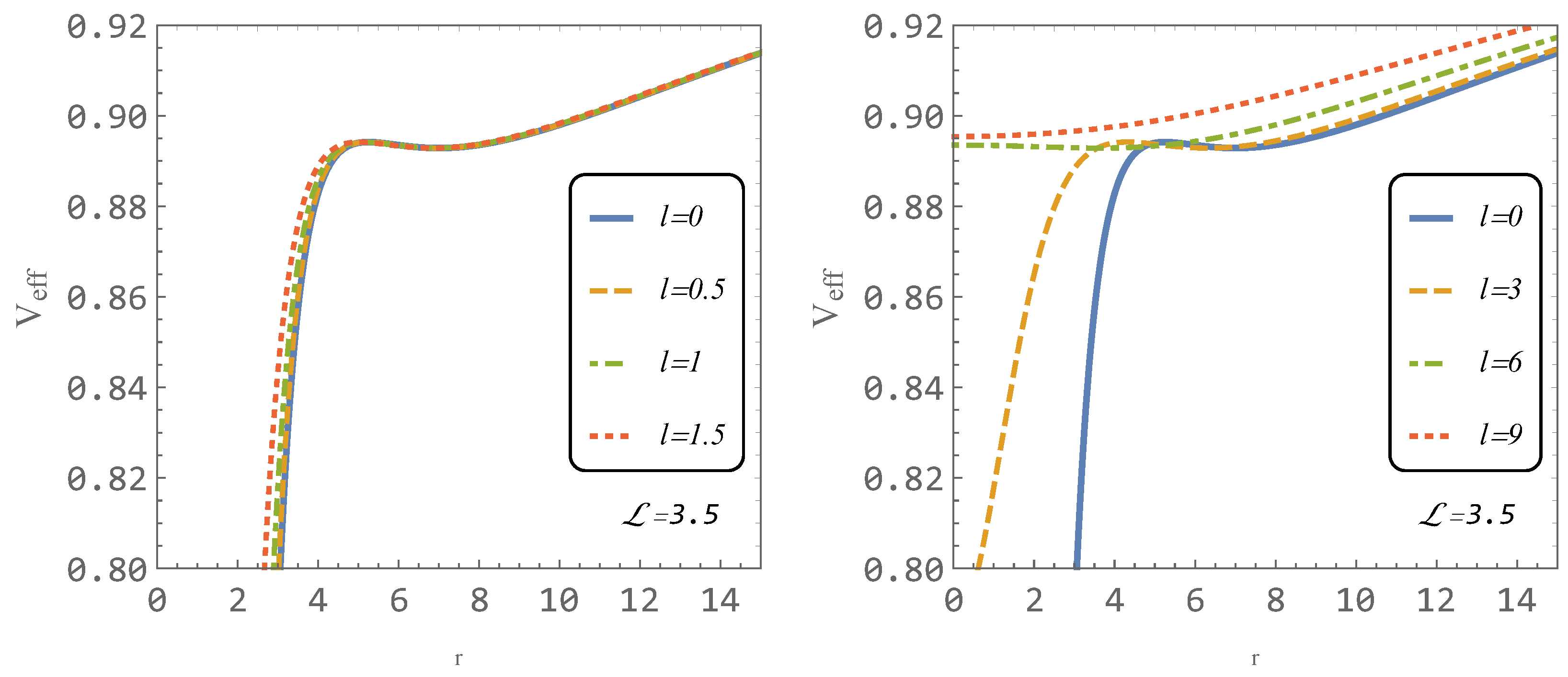
Considering motion of a test particles in the equatorial plane (, ), the character of the radial motion can be governed in the standard way [39] by the effective potential, taking for the massive test particles the form
The character of the effective potential is illustrated for typical situations characteristic for both regular black holes and wormholes in Figure 1. The character of the effective potential is similar to the Schwarzschild case for all the regular black holes and for wormholes with length parameter . In such spacetimes, both stable and unstable circular geodesics are possible. The unstable orbits are limited by the photon circular orbit. However, in the wormhole spacetimes with , only the stable circular geodesics are possible.
The circular geodesics are determined by extrema of the effective potential, i.e., by the condition
implying the radial profile of the particle specific angular momentum in the form
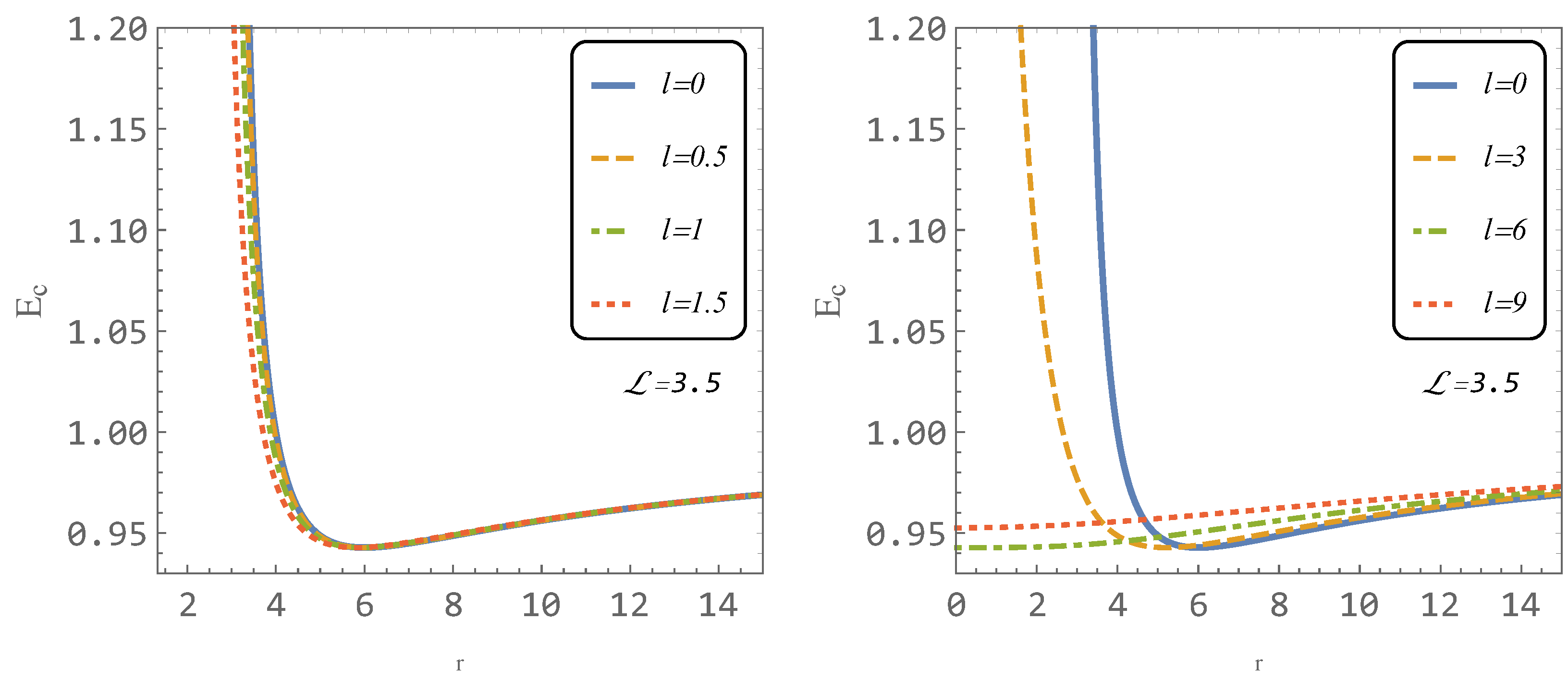
The covariant specific energy of the particle on the circular geodesics, , is determined by the value of the effective potential at the extremal point, and its radial profile is given by the relation
Note that the specific angular momentum can be taken with both signs due to the two (equivalent) possible orientations of the circular motion, while the specific energy has to be taken with only the positive sign, if we consider the particles in positive root states (for details, see [39,40]).
The radial profiles of the specific energy and specific angular momentum of the circular geodesics are for typical values of l illustrated in Figure 2 for regular black holes and Figure 3 for wormholes. Both the specific energy and specific angular momentum radial profiles again demonstrate the fact that for only stable circular orbits are allowed.
The stability of the circular geodesic orbits is determined by the sign of
The marginally stable (innermost) circular geodesic (ISCO) is determined by the condition
that implies the position of the ISCO orbit at the radius
The corresponding specific angular momentum reads
being independent of the scale length parameter l.
Recall that the position of the event horizon of the regular black holes (with ) and the radius of the photon circular geodesic (for ) are determined by the relations [1,28]
The corresponding impact parameter of the photon circular orbits is given by
being independent of the parameter l and having the same form as for photon circular orbit around Schwarzschild black hole.
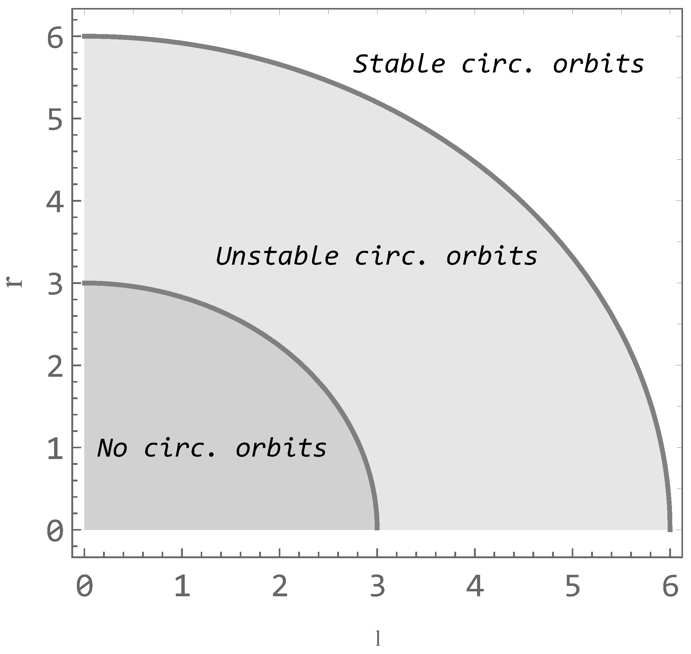
The circular orbits exist where and . There are two curves, and , separating the space into three regions determining existence and position of the photon circular orbits and ISCO (see Figure 4). The region where stable circular orbits are located is bounded by curve . The unstable circular orbits region lays between curves and . There are no circular orbits below curve .
For completeness, we also introduce the angular frequency of the geodesic circular motion as related to the static distant observers defined by the relation —now, the angular frequency, also called the Keplerian angular frequency, is given by formula
The angular frequency can be taken with both signs in accordance with the orientation of the circular motion.
Now, we can study the oscillatory epicyclic motion of test particles orbiting the black hole/wormhole along a stable circular geodesic assuming only small perturbations from the circular orbits allowing for linear (first-order) perturbation analysis.
5. Epicyclic Orbital Motion and Its Frequencies
A test particle slightly displaced from a stable circular orbit at a radius at the equatorial plane starts oscillatory epicyclic motion around the radius and the latitude . We define the coordinate displacement for small perturbations in the radial direction as , and in the latitudinal direction as . The equations governing in the linear perturbation regime the radial and latitudinal epicyclic motion around radius of the stable circular orbit are equivalent to the equation of the harmonic oscillator and take the form [31,41]
where () represents the angular velocity of the radial (latitudinal, or vertical) epicyclic oscillations as measured at the radius of the circular orbit.
The orbital angular frequency of the circular motion is determined by the relation
The angular frequencies of the radial and latitudinal epicyclic motion can be easily calculated by using the Hamiltonian formalism [42,43,44,45]. The Hamiltonian generally defined as
can be split into its dynamic and potential parts
where
The potential part of the Hamiltonian determines the radial and latitudinal epicyclic angular frequencies and due to the relations
Using the relations (1), (16), and (30) in (31) and putting for simplicity , we arrive at the formula
We can see that, as usual in the spherically symmetric spacetimes, the angular frequency of the latitudinal epicyclic oscillations equals the angular frequency of the orbital motion.
Equation (32) gives angular frequencies as measured by a local observer, but we have to find the angular frequencies as measured by static observers at infinity who represent real observers who observe the oscillations from large distance. Therefore, we rescale the locally measured angular frequencies by a corresponding redshift factor related to the orbital motion along the stable circular geodesic at and find
In order to obtain the observed frequencies in the standard units, we have to use the transformation
giving expressions that could be directly used in the fitting to observational data.
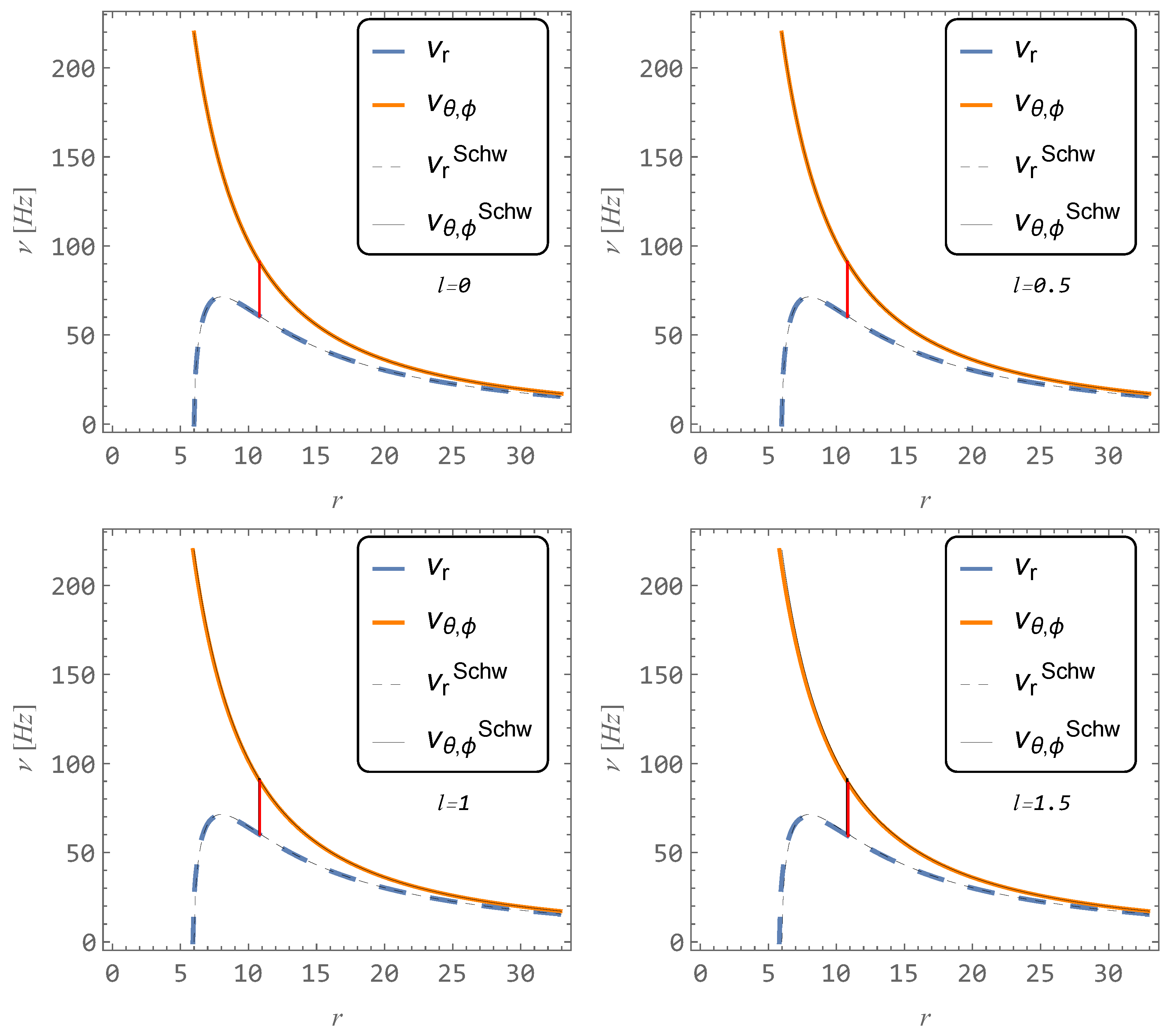
The radial profiles of the orbital (latitudinal epicyclic) and radial epicyclic frequencies are presented for typical values of the scale length parameter l governing the regular black holes in Figure 5 and for wormholes in Figure 6. We can see that, in the case of the regular black holes and wormholes with , the radial profiles of both frequencies are very similar to those related to the Schwarzschild spacetime, and the frequency ratio 3:2 is located very close to the Schwarzschild position [46]. However, for wormholes with , both epicyclic frequencies radial profiles are significantly modified, being starting at the center . The position of the frequency ratio 3:2 is shifted to larger values as compared with the Schwarzschild position, and the shift strongly increases with increasing l.
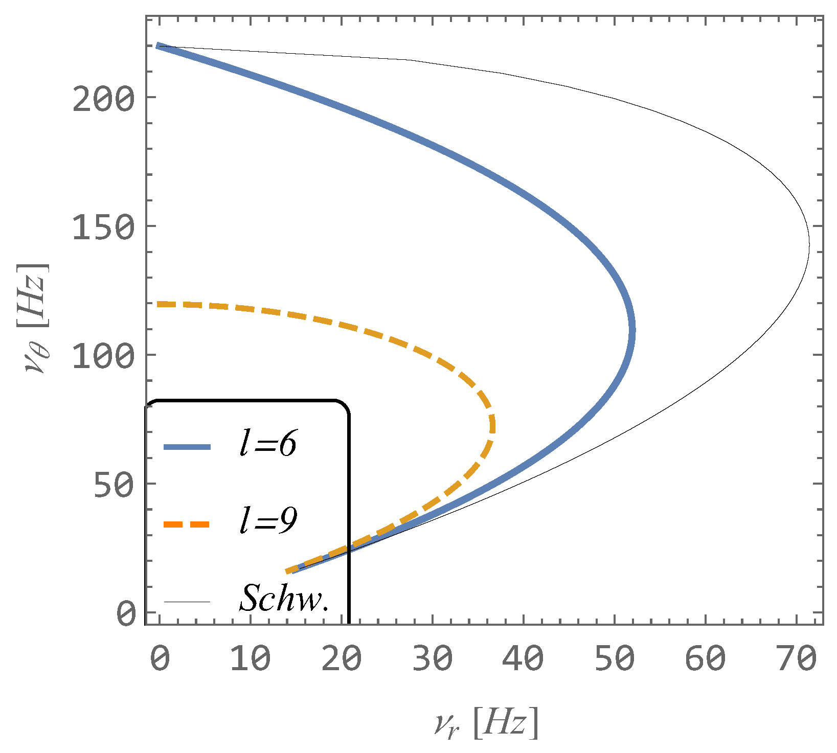
Another view of epicyclic frequencies can be found in Figure 7, where we plot the dependence of on for the values of the parameter . The values were chosen deliberately, as they give the greatest deviation from the result in a purely Schwarzschild background ().
6. The Epicyclic Frequencies Applied in the Epicyclic Resonance Model to Fit the Twin HF QPOs with 3:2 Ratio Observed in Microquasars and around Supermassive Black Holes in Active Galactic Nuclei
In observational astrophysics, the HF QPOs are of very high importance as they enable well founded predictions of parameters of the black holes in accretion systems, i.e., in microquasars representing binary systems containing a stellar mass black hole, or in active galactic nuclei where supermassive black holes are expected. Frequencies of the HF QPOs are in hundreds of Hz in microquasars, and by six or higher orders (up to 10 orders) smaller around the supermassive black holes. Because of the inverse-mass scaling of the observed frequencies that is typical for the relations governing the epicyclic frequencies of the orbital motion [47], the models of HF QPOs related to the orbital motion and its epicyclic oscillations, the so-called geodesic models of HF QPOs, are considered as very promising, especially in connection to the fact that the HF QPOs are often observed in the rational ratio [48], especially in the ratio 3:2 [33], indicating presence of resonant phenomena [49]. A detailed description of the geodesic models can be found in [31]; for generalization with inclusion of an electromagnetic interaction, see the work in [45]. In these models, both upper and lower observed frequencies are assumed to be a combination of the orbital and epicyclic frequencies (note that these frequencies are also relevant for oscillation of slender tori [50]).
The first version of the of the geodesic models is the relativistic precession model proposed in [51] where and . Here, we consider the simple resonance model discussed in [52], where and , demonstrating the role of the scale parameter l in the fitting to observational data related to observed 3:2 twin HF QPOs in microquasars and in HF QPOs observed around supermassive black holes, as discussed recently in [34], where it is demonstrated that the geodesic models are not able to fit data in the case of supermassive black holes. We thus test whether the proposed scale length factor l that could potentially reflect quantum gravity, or different hidden effects, can play a positive role in fitting the data for supermassive black holes.
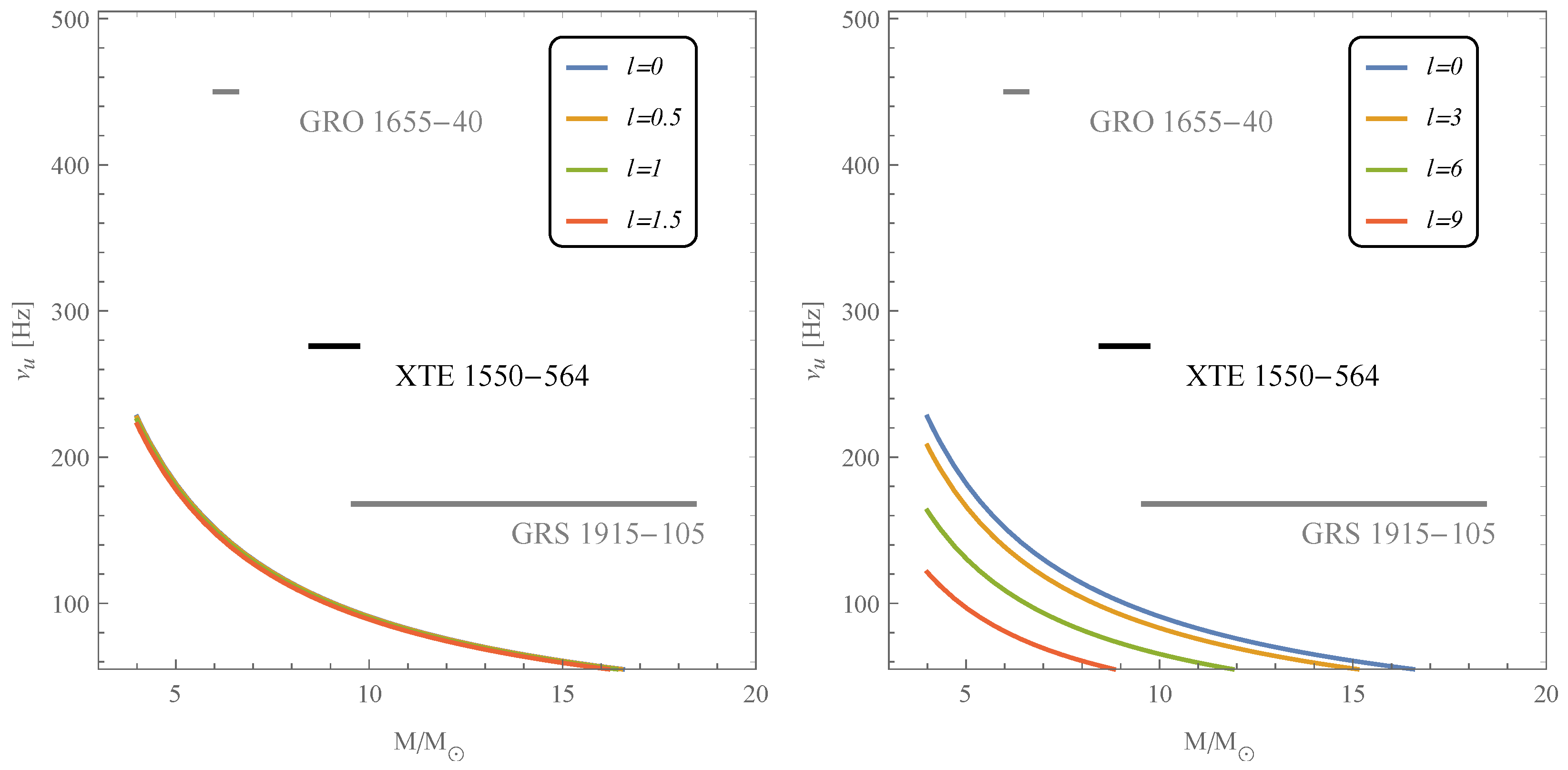
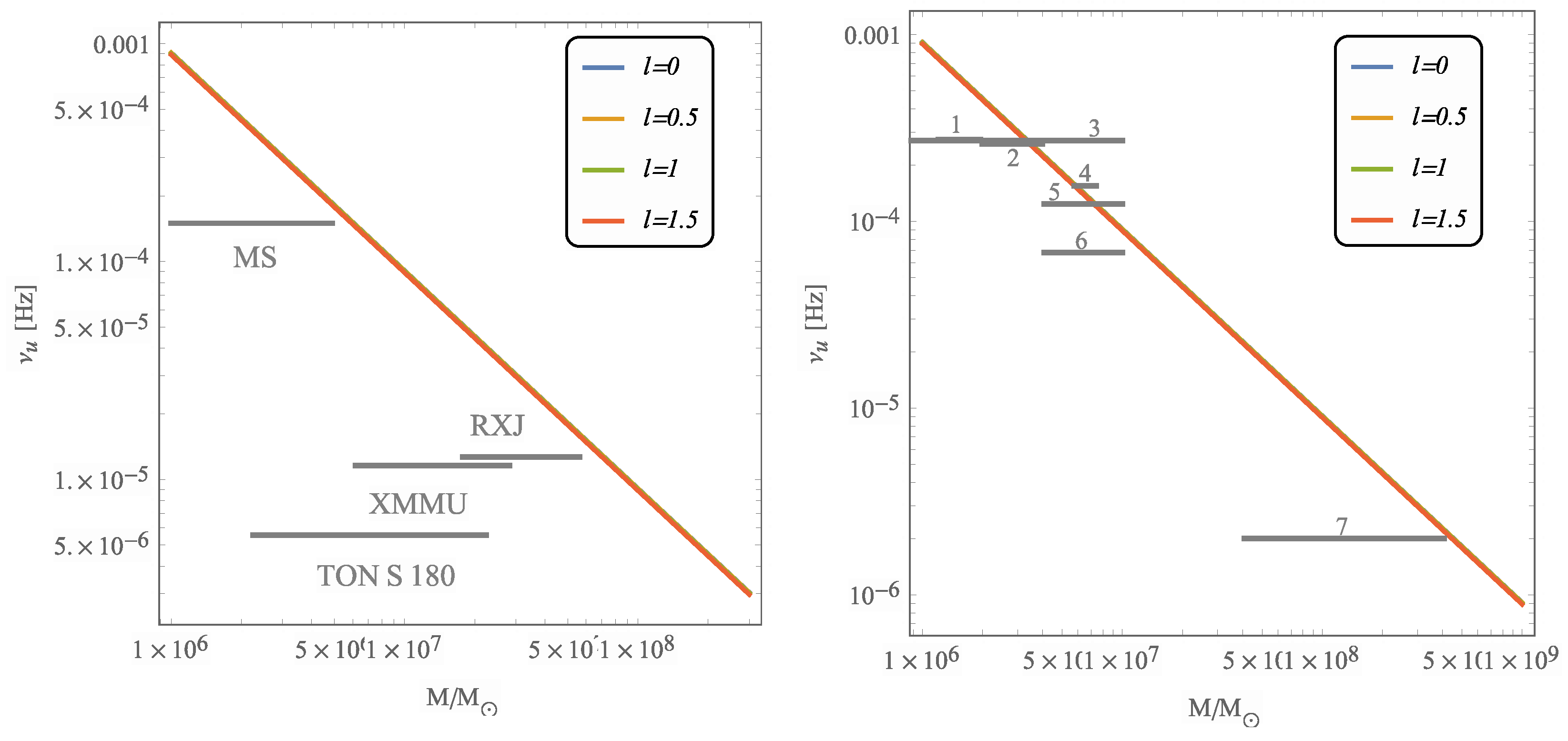
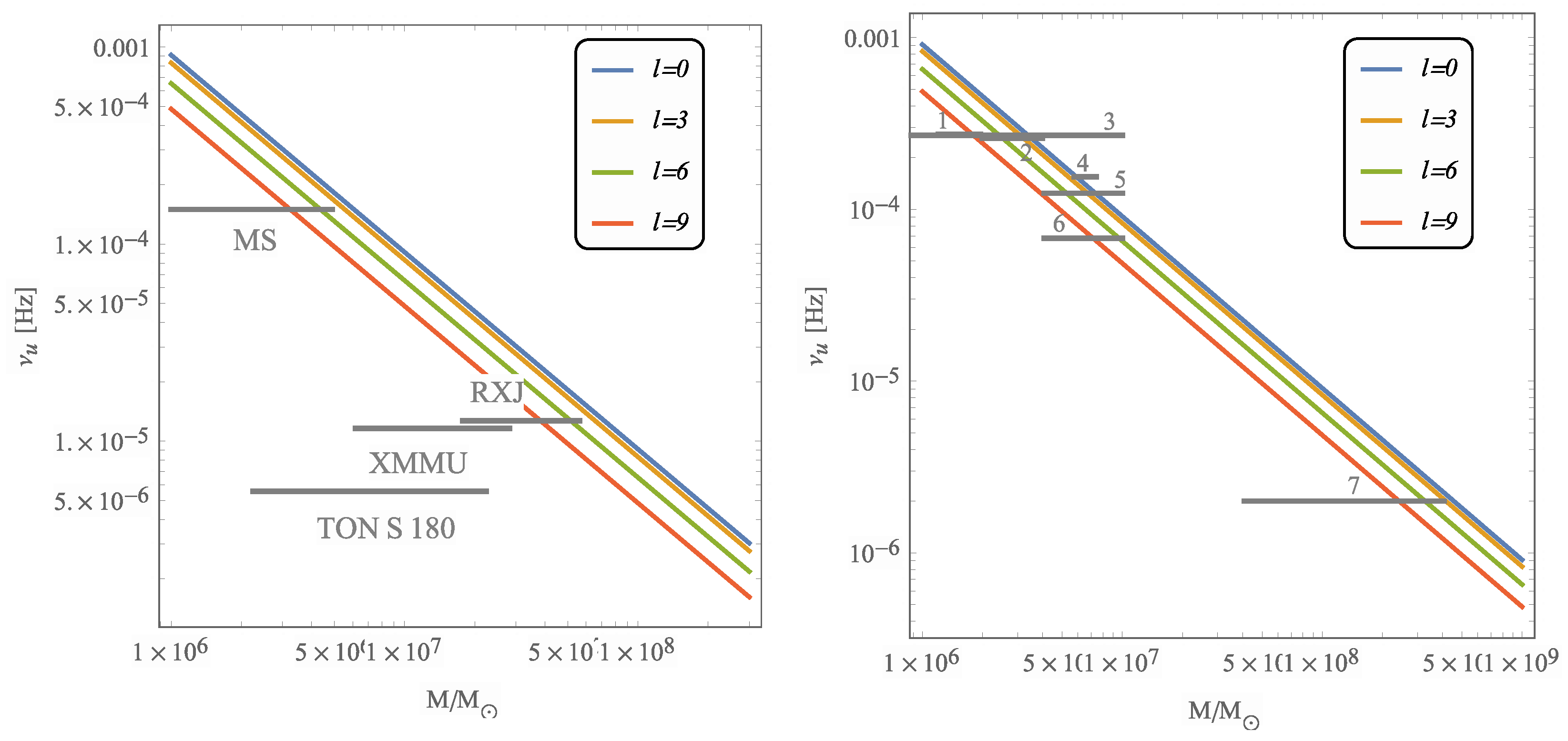
In order to fit the data to the model and obtain restrictions on the parameter l from the restriction on the black hole mass obtained by different methods, we use the method developed in [31]. We consider all the sources discussed in [34]. The results of the fitting procedure are presented in Figure 8 for microquasars and in Figure 9, Figure 10 and Figure 11 for the case of supermassive black holes assumed in active galactic nuclei. The results of the fittings in the case of microquasars are always decreasing the possibility to match the observed data. This discrepancy is increasing with increasing of the length parameter l. On the other hand, we demonstrate the possibility to match the data in all the observed sources in active galactic nuclei, assumed to be supermassive black holes—not by regular black holes, but exclusively by wormholes with sufficiently high value of the length parameter l, determined in dependence on the concrete source. In some sources, the values of l could be slightly higher than , but in some other sources they have to be very high, . In the case of large values of l, the fitting to the data implies a position of the resonant oscillation in large distance from the center of the wormhole.
7. Conclusions
We give frequencies of the epicyclic oscillatory motion around stable circular geodesics in the field of regular black holes and wormholes governed by the Simpson–Visser meta-geometry describing them by a unique scale length parameter that potentially could reflect some hidden effect, e.g., of quantum gravity. The epicyclic frequencies are applied in the special version of the geodesic models of the twin HF QPOs, namely the epicyclic resonance model. We demonstrate that, in the case of microquasars, the length parameter l has the general tendency to decrease the possibility to find the fits, but, in the case of the frequencies observed around assumed supermassive black holes in active galactic nuclei, the parameter acts in positive way, and, for wormholess with sufficiently high values of l, the fitting is possible for all observed sources discussed in [34]. Of course, the values of l are very high in many cases, being astrophysically unrealistic, but possible inclusion of the rotation of the wormholes introduced in [2] could lead to significant improvement and decrease the length parameter l. Another positive influence could be due to the dark matter concentrated around the wormhole.
Of course, in making definite conclusions, some additional phenomena have to be considered such as the precession frequencies of some orbiting mass [53] and the optical phenomena such as shadow [54,55].
We can conclude that our positive results for data fitting obtained in the case of supermassive black holes favor supermassive wormholes in comparison with regular black holes and could be considered as a clear possibility to observationally distinguish wormholes from black holes—of strong significance from this point of view is the case of large values of l when the oscillations should occur at a rather large distance from the wormhole, as measured in the gravitational radius, contrary to the black hole case when the resonance would occur at a small distance from the black hole. For large values of l, we could even expect some influence on the estimation of the supermassive throat object, namely its mass. However, these estimates are usually made for phenomena considered in the weak field limit, at a very large distance from the central object, for , and even for values of we can neglect the role of l at such large distances.
Author Contributions
Funding
Z.S. was supported by the Czech Science Foundation grant No. 19-03950S.
Acknowledgments
The authors acknowledge the institutional support of the Institute of Physics at the Silesian University in Opava.
Conflicts of Interest
The authors declare no conflict of interest.
References
- Simpson, A.; Visser, M. Black-bounce to traversable wormhole. JCAP 2019, 2019, 42. [Google Scholar] [CrossRef] [Green Version]
- Mazza, J.; Franzin, E.; Liberati, S. A novel family of rotating black hole mimickers. JCAP 2021, 2021, 82. [Google Scholar] [CrossRef]
- Morris, M.S.; Thorne, K.S. Wormholes in spacetime and their use for interstellar travel: A tool for teaching general relativity. Am. J. Phys. 1988, 56, 395–412. [Google Scholar] [CrossRef] [Green Version]
- Morris, M.S.; Thorne, K.S.; Yurtsever, U. Wormholes, time machines, and the weak energy condition. Phys. Rev. Lett. 1988, 61, 1446–1449. [Google Scholar] [CrossRef] [PubMed] [Green Version]
- Bronnikov, K.A.; Dehnen, H.; Melnikov, V.N. Regular black holes and black universes. Gen. Relativ. Gravit. 2007, 39, 973–987. [Google Scholar] [CrossRef] [Green Version]
- Visser, M. Traversable wormholes from surgically modified Schwarzschild spacetimes. Nucl. Phys. B 1989, 328, 203–212. [Google Scholar] [CrossRef] [Green Version]
- Poisson, E.; Visser, M. Thin-shell wormholes: Linearization stability. Phys. Rev. D 1995, 52, 7318–7321. [Google Scholar] [CrossRef] [Green Version]
- Visser, M. Traversable wormholes: Some simple examples. Phys. Rev. D 1989, 39, 3182–3184. [Google Scholar] [CrossRef] [PubMed] [Green Version]
- Svítek, O.; Tahamtan, T. Nonsymmetric dynamical thin-shell wormhole in Robinson-Trautman class. Eur. Phys. J. C 2018, 78, 167. [Google Scholar] [CrossRef] [Green Version]
- Harko, T.; Lobo, F.S.N.; Mak, M.K.; Sushkov, S.V. Modified-gravity wormholes without exotic matter. Phys. Rev. D 2013, 87, 067504. [Google Scholar] [CrossRef] [Green Version]
- Maldacena, J.; Milekhin, A.; Popov, F. Traversable wormholes in four dimensions. arXiv 2018, arXiv:1807.04726. [Google Scholar]
- Blázquez-Salcedo, J.L.; Knoll, C. Constructing spherically symmetric Einstein-Dirac systems with multiple spinors: Ansatz, wormholes and other analytical solutions. Eur. Phys. J. C 2020, 80, 174. [Google Scholar] [CrossRef]
- Blázquez-Salcedo, J.L.; Knoll, C.; Radu, E. Traversable Wormholes in Einstein-Dirac-Maxwell Theory. Phys. Rev. Lett. 2021, 126, 101102. [Google Scholar] [CrossRef] [PubMed]
- Tursunov, A.; Zajaček, M.; Eckart, A.; Kološ, M.; Britzen, S.; Stuchlík, Z.; Czerny, B.; Karas, V. Effect of Electromagnetic Interaction on Galactic Center Flare Components. Astrophys. J. 2020, 897, 99. [Google Scholar] [CrossRef]
- Event Horizon Telescope Collaboration. First M87 Event Horizon Telescope Results. I. The Shadow of the Supermassive Black Hole. Astrophys. J. Lett. 2019, 875, L1. [Google Scholar] [CrossRef]
- Gimon, E.G.; Hořava, P. Astrophysical violations of the Kerr bound as a possible signature of string theory. Phys. Lett. B 2009, 672, 299–302. [Google Scholar] [CrossRef] [Green Version]
- Stuchlík, Z.; Hledík, S.; Truparová, K. Evolution of Kerr superspinars due to accretion counterrotating thin discs. Class. Quantum Gravity 2011, 28, 155017. [Google Scholar] [CrossRef]
- Stuchlík, Z.; Schee, J. Observational phenomena related to primordial Kerr superspinars. Class. Quantum Gravity 2012, 29, 065002. [Google Scholar] [CrossRef]
- Stuchlík, Z.; Schee, J. Appearance of Keplerian discs orbiting Kerr superspinars. Class. Quantum Gravity 2010, 27, 215017. [Google Scholar] [CrossRef] [Green Version]
- Stuchlik, Z. Equatorial Circular Orbits and the Motion of the Shell of Dust in the Field of a Rotating Naked Singularity. Bull. Astron. Inst. Czechoslov. 1980, 31, 129. [Google Scholar]
- Stuchlík, Z.; Schee, J. Ultra-high-energy collisions in the superspinning Kerr geometry. Class. Quantum Gravity 2013, 30, 075012. [Google Scholar] [CrossRef]
- Blaschke, M.; Stuchlík, Z. Efficiency of the Keplerian accretion in braneworld Kerr-Newman spacetimes and mining instability of some naked singularity spacetimes. Phys. Rev. D 2016, 94, 086006. [Google Scholar] [CrossRef] [Green Version]
- Stuchlík, Z.; Blaschke, M.; Schee, J. Particle collisions and optical effects in the mining Kerr-Newman spacetimes. Phys. Rev. D 2017, 96, 104050. [Google Scholar] [CrossRef] [Green Version]
- Abdujabbarov, A.; Juraev, B.; Ahmedov, B.; Stuchlík, Z. Shadow of rotating wormhole in plasma environment. Astrophys. Space Sci. 2016, 361, 226. [Google Scholar] [CrossRef]
- Deligianni, E.; Kunz, J.; Nedkova, P.; Yazadjiev, S.; Zheleva, R. Quasi-periodic oscillations from the accretion disk around rotating traversable wormholes. arXiv 2021, arXiv:2103.13504. [Google Scholar]
- Zhou, T.-Y.; Xie, Y. Precessing and periodic motions around a black-bounce/traversable wormhole. Eur. Phys. J. C 2020, 80, 1070. [Google Scholar] [CrossRef]
- Guerrero, M.; Olmo, G.J.; Rubiera-Garcia, D.; Sáez-Chillón Gómez, D. Shadows and optical appearance of black bounces illuminated by a thin accretion disk. arXiv 2021, arXiv:2105.15073. [Google Scholar]
- Stuchlík, Z.; Schee, J. Appearance of Keplerian discs orbiting on both sides of a reflection-symmetries wormhole. Eur. Phys. J. C 2021. submitted. [Google Scholar]
- Churilova, M.S.; Stuchlík, Z. Ringing of the regular black-hole/wormhole transition. Class. Quantum Gravity 2020, 37, 075014. [Google Scholar] [CrossRef] [Green Version]
- Bronnikov, K.A.; Konoplya, R.A. Echoes in brane worlds: Ringing at a black hole-wormhole transition. Phys. Rev. D 2020, 101, 064004. [Google Scholar] [CrossRef] [Green Version]
- Stuchlík, Z.; Kotrlová, A.; Török, G. Multi-resonance orbital model of high-frequency quasi-periodic oscillations: Possible high-precision determination of black hole and neutron star spin. Astron. Astrophys. 2013, 552, A10. [Google Scholar] [CrossRef] [Green Version]
- Stuchlík, Z.; Kološ, M.; Kovář, J.; Slaný, P.; Tursunov, A. Influence of Cosmic Repulsion and Magnetic Fields on Accretion Disks Rotating around Kerr Black Holes. Universe 2020, 6, 26. [Google Scholar] [CrossRef] [Green Version]
- Török, G.; Kotrlová, A.; Šrámková, E.; Stuchlík, Z. Confronting the models of 3:2 quasiperiodic oscillations with the rapid spin of the microquasar GRS 1915+105. Astron. Astrophys. 2011, 531, A59. [Google Scholar] [CrossRef] [Green Version]
- Smith, K.L.; Tandon, C.R.; Wagoner, R.V. Confrontation of Observation and Theory: High-frequency QPOs in X-ray Binaries, Tidal Disruption Events, and Active Galactic Nuclei. Astrophys. J. 2021, 906, 92. [Google Scholar] [CrossRef]
- Rovelli, C.; Vidotto, F. Planck stars. Int. J. Mod. Phys. D 2014, 23, 1442026. [Google Scholar] [CrossRef]
- Haggard, H.M.; Rovelli, C. Quantum-gravity effects outside the horizon spark black to white hole tunneling. Phys. Rev. D 2015, 92, 104020. [Google Scholar] [CrossRef] [Green Version]
- Malafarina, D. Classical Collapse to Black Holes and Quantum Bounces: A Review. Universe 2017, 3, 48. [Google Scholar] [CrossRef] [Green Version]
- Carballo-Rubio, R.; Di Filippo, F.; Liberati, S.; Visser, M. Geodesically complete black holes. Phys. Rev. D 2020, 101, 084047. [Google Scholar] [CrossRef]
- Misner, C.W.; Thorne, K.S.; Wheeler, J.A. Gravitation; W. H. Freeman Princeton University Press: Princeton, NJ, USA, 1973. [Google Scholar]
- Bicak, J.; Suchlik, Z.; Balek, V. The Motion of Charged Particles in the Field of Rotating Charged Black Holes and Naked Singularities. I. The General Features of the Radial Motion and the Motion Along the Axis of Symmetry. Bull. Astron. Inst. Czechoslov. 1989, 40, 65. [Google Scholar]
- Török, G.; Stuchlík, Z. Radial and vertical epicyclic frequencies of Keplerian motion in the field of Kerr naked singularities. Comparison with the black hole case and possible instability of naked-singularity accretion discs. Astron. Astrophys. 2005, 437, 775–788. [Google Scholar] [CrossRef]
- Kološ, M.; Stuchlík, Z.; Tursunov, A. Quasi-harmonic oscillatory motion of charged particles around a Schwarzschild black hole immersed in a uniform magnetic field. Class. Quantum Gravity 2015, 32, 165009. [Google Scholar] [CrossRef] [Green Version]
- Tursunov, A.; Stuchlík, Z.; Kološ, M. Circular orbits and related quasiharmonic oscillatory motion of charged particles around weakly magnetized rotating black holes. Phys. Rev. D 2016, 93, 084012. [Google Scholar] [CrossRef] [Green Version]
- Stuchlík, Z.; Kološ, M. Acceleration of the charged particles due to chaotic scattering in the combined black hole gravitational field and asymptotically uniform magnetic field. Eur. Phys. J. C 2016, 76, 32. [Google Scholar] [CrossRef] [Green Version]
- Kološ, M.; Tursunov, A.; Stuchlík, Z. Possible signature of the magnetic fields related to quasi-periodic oscillations observed in microquasars. Eur. Phys. J. C 2017, 77, 860. [Google Scholar] [CrossRef]
- Kato, S.; Fukue, J.; Mineshige, S. Black-Hole Accretion Disks; Kyoto University Press: Kyoto, Japan, 1998. [Google Scholar]
- Remillard, R.A.; McClintock, J.E. X-ray Properties of Black-Hole Binaries. Annu. Rev. Astron. Astrophys. 2006, 44, 49–92. [Google Scholar] [CrossRef] [Green Version]
- McClintock, J.E.; Remillard, R.A. Black hole binaries. In Compact Stellar X-ray Sources; Cambridge University Press: Cambridge, UK, 2006; Volume 39, pp. 157–213. [Google Scholar]
- Kluzniak, W.; Abramowicz, M.A. Strong-Field Gravity and Orbital Resonance in Black Holes and Neutron Stars—kHz Quasi-Periodic Oscillations (QPO). Acta Phys. Pol. B 2001, 32, 3605. [Google Scholar]
- Rezzolla, L.; Yoshida, S.; Zanotti, O. Oscillations of vertically integrated relativistic tori - I. Axisymmetric modes in a Schwarzschild space-time. Mon. Not. RAS 2003, 344, 978–992. [Google Scholar] [CrossRef] [Green Version]
- Stella, L.; Vietri, M.; Morsink, S.M. Correlations in the Quasi-periodic Oscillation Frequencies of Low-Mass X-ray Binaries and the Relativistic Precession Model. Astrophys. J. Lett. 1999, 524, L63–L66. [Google Scholar] [CrossRef] [Green Version]
- Török, G.; Abramowicz, M.A.; Kluźniak, W.; Stuchlík, Z. The orbital resonance model for twin peak kHz quasi periodic oscillations in microquasars. Astron. Astrophys. 2005, 436, 1–8. [Google Scholar] [CrossRef]
- Rizwan, M.; Jamil, M.; Jusufi, K. Distinguishing a Kerr-like black hole and a naked singularity in perfect fluid dark matter via precession frequencies. Phys. Rev. D 2019, 99, 024050. [Google Scholar] [CrossRef] [Green Version]
- Bambi, C. Can the supermassive objects at the centers of galaxies be traversable wormholes? The first test of strong gravity for mm/sub-mm very long baseline interferometry facilities. Phys. Rev. D 2013, 87, 107501. [Google Scholar] [CrossRef] [Green Version]
- Nedkova, P.G.; Tinchev, V.K.; Yazadjiev, S.S. Shadow of a rotating traversable wormhole. Phys. Rev. D 2013, 88, 124019. [Google Scholar] [CrossRef] [Green Version]
Figure 1.
Effective potentials of test particles for characteristic values of the length parameter l and . Values of giving regular black holes are on the left panel, while values of giving wormholes (except the Schwarzschild case ) are on the right panel.
Figure 1.
Effective potentials of test particles for characteristic values of the length parameter l and . Values of giving regular black holes are on the left panel, while values of giving wormholes (except the Schwarzschild case ) are on the right panel.

Figure 2.
The radial profiles of the specific energy of test particle for characteristic values of the parameter l and . Values of giving regular black holes are on the left panel, while values of giving wormholes (except giving for comparison the Schwarzschild black hole) are on the right panel.
Figure 2.
The radial profiles of the specific energy of test particle for characteristic values of the parameter l and . Values of giving regular black holes are on the left panel, while values of giving wormholes (except giving for comparison the Schwarzschild black hole) are on the right panel.

Figure 3.
The radial profiles of the specific angular momentum of test particle for characteristic values of the parameter l and . Values of l giving regular black holes are on the left panel, while values of l giving wormholes (except giving the Schwarzschild black hole) are on the right panel.
Figure 3.
The radial profiles of the specific angular momentum of test particle for characteristic values of the parameter l and . Values of l giving regular black holes are on the left panel, while values of l giving wormholes (except giving the Schwarzschild black hole) are on the right panel.

Figure 4.
The structure of circular orbits in wormhole spacetime with .

Figure 5.
Epicyclic frequencies radial profiles for characteristic values of the parameter l in units of M giving regular black holes and . Vertical black line indicates frequency ratio 3:2 for Schwarzschild case and red for given l (here both vertical lines almost coincide).
Figure 5.
Epicyclic frequencies radial profiles for characteristic values of the parameter l in units of M giving regular black holes and . Vertical black line indicates frequency ratio 3:2 for Schwarzschild case and red for given l (here both vertical lines almost coincide).

Figure 6.
Epicyclic frequencies radial profiles for characteristic values of the parameter l in units of M giving wormholes (except corresponding to Schwarzschild black hole) and . Vertical black line indicates frequencies ratio 3:2 for Schwarzschild case and red for given l.
Figure 6.
Epicyclic frequencies radial profiles for characteristic values of the parameter l in units of M giving wormholes (except corresponding to Schwarzschild black hole) and . Vertical black line indicates frequencies ratio 3:2 for Schwarzschild case and red for given l.

Figure 7.
The dependence of on for the values of the parameter giving wormholes (except corresponding to the Schwarzschild black hole); .
Figure 7.
The dependence of on for the values of the parameter giving wormholes (except corresponding to the Schwarzschild black hole); .

Figure 8.
Fit of 3:2 frequencies ratio to mass estimate of microquasars for various parameter l by using the epicyclic resonance model. This model is used in all the following figures of fits. Values of l giving black hole are on the left panel, while values of l giving wormholes (except , which gives the Schwarzschild black hole) are on the right panel.

Figure 9.
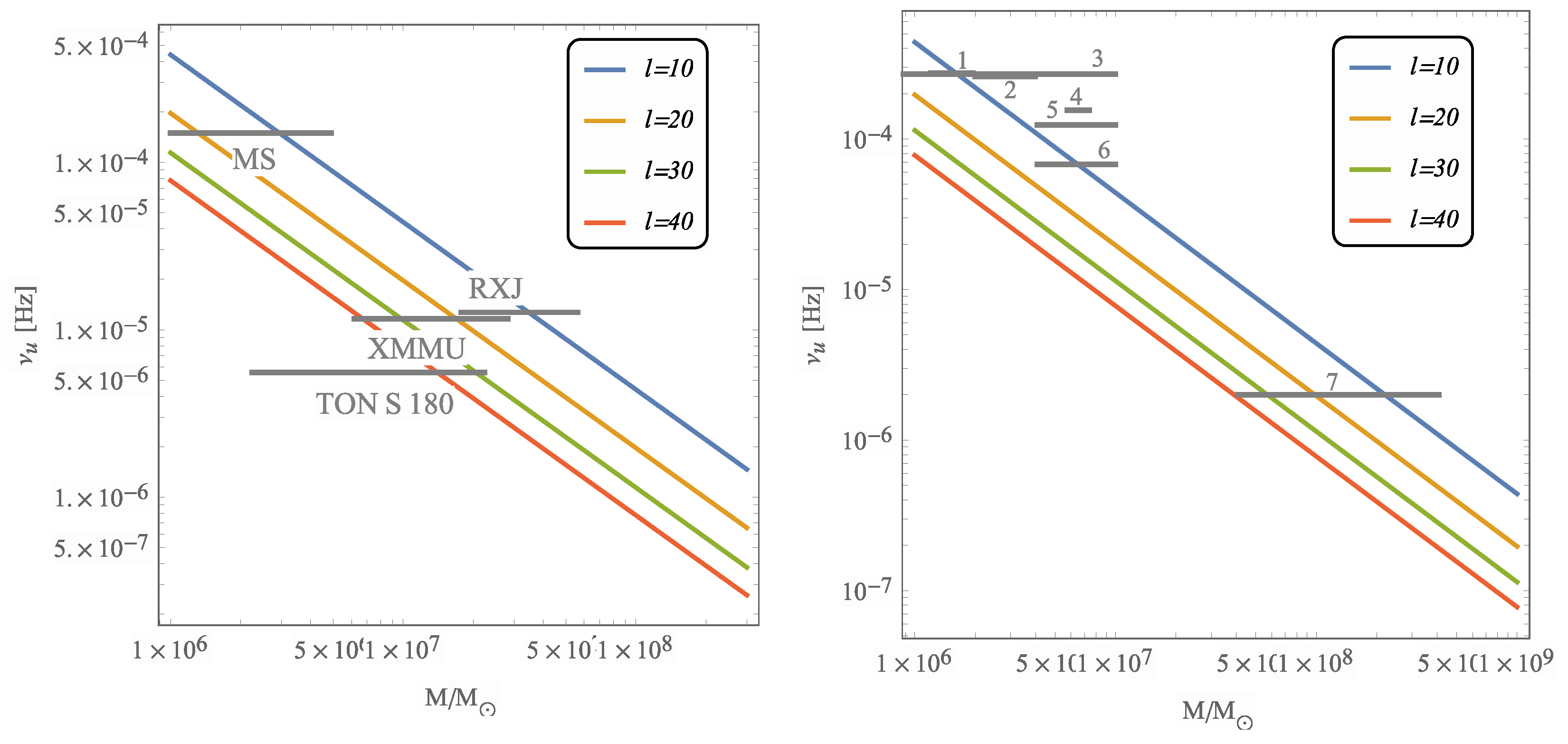
Fit of 3:2 frequencies ratio to mass estimate of assumed supermassive black holes in active galactic nuclei for various values of the parameter l giving regular black holes. The sources with unknown rotation estimates are marked on the left panel. On the right panel are sources with known estimate of spin listed in Table 1 (cf. [34]). Notice that the curves almost coincide.
Figure 9.
Fit of 3:2 frequencies ratio to mass estimate of assumed supermassive black holes in active galactic nuclei for various values of the parameter l giving regular black holes. The sources with unknown rotation estimates are marked on the left panel. On the right panel are sources with known estimate of spin listed in Table 1 (cf. [34]). Notice that the curves almost coincide.

Figure 10.
Fit of 3:2 frequencies ratio to mass estimate of assumed supermassive black holes in active galactic nuclei for various values of the parameter l giving Simpson–Visser wormholes. Sources with unknown rotation estimates are marked on the left panel. On the right panel are sources with known estimate of spin listed in Table 1 (cf. [34]).

Figure 11.
Fit of 3:2 frequencies ratio to mass estimate of assumed supermassive black holes in active galactic nuclei for various values of the parameter l giving wormholes. Sources with unknown rotation estimates are marked in the left panel. On the right panel are sources with a known estimate of spin listed in Table 1 (cf. [34]).


Publisher’s Note: MDPI stays neutral with regard to jurisdictional claims in published maps and institutional affiliations. |
© 2021 by the authors. Licensee MDPI, Basel, Switzerland. This article is an open access article distributed under the terms and conditions of the Creative Commons Attribution (CC BY) license (https://creativecommons.org/licenses/by/4.0/).
Share and Cite
MDPI and ACS Style
Stuchlík, Z.; Vrba, J. Epicyclic Oscillations around Simpson–Visser Regular Black Holes and Wormholes. Universe 2021, 7, 279. https://0-doi-org.brum.beds.ac.uk/10.3390/universe7080279
AMA Style
Stuchlík Z, Vrba J. Epicyclic Oscillations around Simpson–Visser Regular Black Holes and Wormholes. Universe. 2021; 7(8):279. https://0-doi-org.brum.beds.ac.uk/10.3390/universe7080279
Chicago/Turabian StyleStuchlík, Zdeněk, and Jaroslav Vrba. 2021. "Epicyclic Oscillations around Simpson–Visser Regular Black Holes and Wormholes" Universe 7, no. 8: 279. https://0-doi-org.brum.beds.ac.uk/10.3390/universe7080279
Note that from the first issue of 2016, this journal uses article numbers instead of page numbers. See further details here.