
Bayesian Methods for Inferring Missing Data in the BATSE Catalog of Short Gamma-Ray Bursts


Department of Physics, The University of Texas, Arlington, TX 76010, USA
*
Author to whom correspondence should be addressed.
Universe 2022, 8(5), 267; https://0-doi-org.brum.beds.ac.uk/10.3390/universe8050267
Submission received: 12 March 2022
/
Revised: 21 April 2022
/
Accepted: 25 April 2022
/
Published: 28 April 2022
(This article belongs to the Special Issue Gamma-Ray Bursts: Observational and Theoretical Prospects in the Era of Multi-Messenger Astronomy)
Abstract
:The knowledge of the redshifts of Short-duration Gamma-Ray Bursts (SGRBs) is essential for constraining their cosmic rates and thereby the rates of related astrophysical phenomena, particularly Gravitational Wave Radiation (GWR) events. Many of the events detected by gamma-ray observatories (e.g., BATSE, Fermi, and Swift) lack experimentally measured redshifts. To remedy this, we present and discuss a generic data-driven probabilistic modeling framework to infer the unknown redshifts of SGRBs in the BATSE catalog. We further explain how the proposed probabilistic modeling technique can be applied to newer catalogs of SGRBs and other astronomical surveys to infer the missing data in the catalogs.
1. Introduction
The discovery of the first Gravitational Wave Radiation (GWR) event in 2015 [1,2] and the first joint detection of gravitational and electromagnetic radiation from a binary neutron star merger in 2017 [3] have revolutionized multimessenger astronomy and resulted in the 2017 Physics Nobel Prize. These observations have given credibility to the hypothesis of binary neutron star (BNS) mergers as the primary progenitors of Short Gamma-Ray Bursts (SGRBs). Other channels of SGRB formation include neutron stars—black hole or binary black hole mergers. Unlike Long Gamma-Ray Bursts (LGRBs), which are believed to be due to the collapse of supermassive stars and are frequently associated with core-collapse supernovae [4], the light curves of SGRBs are comprised of short-hard intense gamma-ray pulses that generally last a few milliseconds to seconds.
A question of great interest in the field of GWR astronomy concerns the cosmic rates of GWRs and the fraction of detectable events with the current and planned GWR detectors [5]. LGRBs and SGRBs are among the major sources of GWR events. Therefore, knowledge of the cosmic rates of GRBs can yield tight constraints on the cosmic rates of GWR events. The challenge, however, lies in quantifying the population properties and the cosmic rates of GRBs. Unraveling the physics and the intrinsic properties of GRBs requires knowledge of their distances from Earth represented by the quantity known as the cosmological redshift (z). Despite significant progress made over the past two decades, most events detected by the existing gamma-ray observatories lack measured redshifts. For example, less than of the entire catalog of >3000 GRBs detected by the Gamma-ray Burst Monitor (GBM) onboard the Fermi Gamma-ray Space Telescope have measured redshifts, and even fewer of those with measured redshifts belong to the class of SGRBs, a primary GWR formation channel. While there seems to exist a consensus on the range of the redshift distributions of LGRBs and SGRBs [6,7,8,9], the shapes of the distributions and the knowledge of the redshifts of individual events remain hotly debated [9] and elusive. Previous studies have already utilized the phenomenologically discovered prompt gamma-ray correlations to derive pseudo-redshifts for a certain fraction of events in the second-largest catalog of GRBs available to this date, homogeneously detected by the BATSE Large Area Detectors onboard the now-defunct Compton Gamma-Ray Observatory [10,11,12,13]. More recent studies have applied similar concepts and ideas to the problem of estimating the unknown redshifts of GRBs in the Fermi-GBM catalog [14,15].
These methods, however, can lead to highly biased estimates of the unknown redshifts of GRBs where the discovered high-energy correlations result from a small calibration sample. The calibration samples are typically the brightest detected GRBs whose redshift measurements have been feasible. Such small samples are often collected from multiple heterogeneous surveys and potentially neither represent the unobserved intrinsic cosmic population of GRBs nor the complete observed sample (with or without measured redshifts). More importantly, the potential effects of the detector threshold and sample incompleteness on the proposed phenomenological correlations are poorly understood. These unknown effects and systematic biases manifest themselves in predicted redshift values that are highly inconsistent with the estimates obtained from other independent methods; examples of which are well studied in the literature [16,17,18,19].
In this article, we propose and lay out the details of a data-driven approach to reconstructing the missing redshift and other information in GRB catalogs. The proposed methodology is generic, is applicable to any astronomical or other type of datasets, and opens the venue toward further quantification of the answers to some of the major questions in GRB research, including but not limited to: What are the cosmic rates of Short- and Long-duration GRBs? Can the observational properties of GRBs be used as cosmological standard candles? Is there a reliable indirect method of inferring the redshifts of GRBs in real time? Are there any deviations in the cosmic rates of LGRBs from the Star Formation Rate? To explain the proposed probabilistic framework, we particularly focus on the BATSE catalog of 565 SGRBs due to the simplicity of the BATSE triggering mechanism. Despite the extremely large uncertainties in the BATSE SGRBs’ observational data, we show the feasibility of setting reasonable constraints on the individual redshifts of most BATSE SGRBs. Although we frequently refer to the Fermi-GBM and Swift-BAT catalogs of GRBs in discussions, we leave a complete treatment of these catalogs to future studies. This study is a continuation of a previous similar study of the BATSE LGRBs catalog [1].
2. Methodology
Our proposed approach to reconstructing the missing data in GRB catalogs comprises three major steps:
Firstly, describe the probabilistic foundations of our proposed Bayesian approach to inferring missing data from the available observational catalog(s) combined with any prior knowledge from independent resources. Such techniques should naturally incorporate all sources of uncertainty into the analysis.
Secondly, we develop a detailed minimally biased model of the detection process of GRBs. Such careful mathematical modeling of gamma-ray photon detectors is crucial for an accurate study of the population properties of GRBs and the estimation of their cosmic rates.
Lastly, we introduce a probabilistic framework for calibrating, validating, and selecting the most plausible model for the population properties of the prompt gamma-ray emission of GRBs, which can be subsequently used to infer the unknown missing data in GRB catalogs, most importantly, the unknown redshifts of the individual GRBs. A more detailed explanation of this process is given in Section 2.1, Section 2.2 and Section 2.3.
2.1. Development of the Statistical Techniques
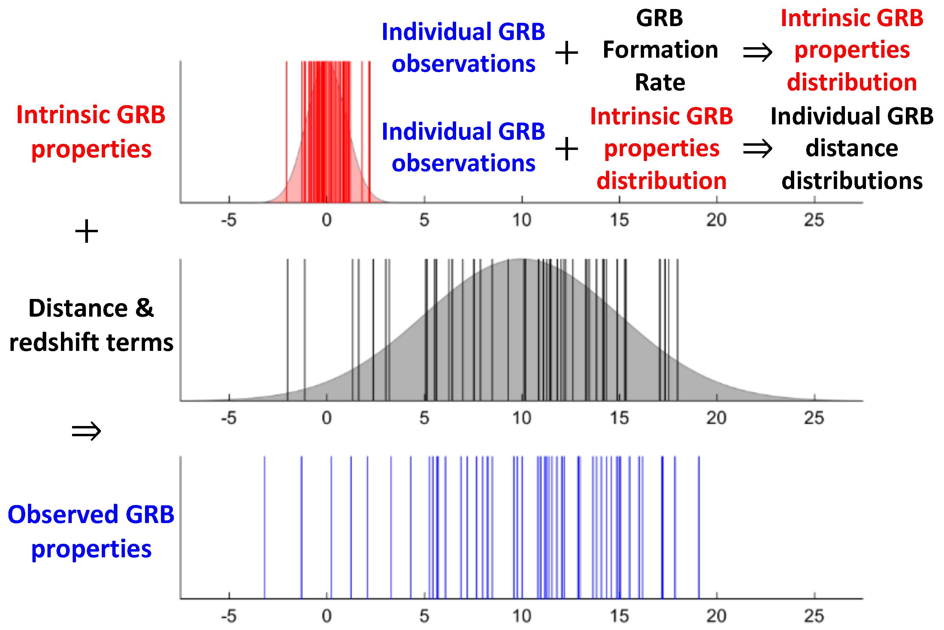
The essence of the proposed approach to estimating the missing data, specifically the unknown redshifts of GRBs, is summarized in Figure 1. For illustration, consider a toy model where the observed properties of one GRB class (e.g., SGRBs) are collectively represented by the single blue-colored lines in this figure. Each blue line represents one GRB event. If we knew the redshifts of these individual events, represented by the black lines in the middle subplot, we would be able to determine, with high precision, the intrinsic properties of all detected GRBs, represented by the red lines in the top subplot. The background shaded areas in the top and middle subplots represent the generating distributions of the corresponding lines in the foreground. Two approaches to inferring the cosmic rates of GRBs and individual redshifts can be taken, depending on the state of knowledge of individual GRB redshifts in a given GRB catalog.
2.1.1. Modeling Scenario 1
In the presence of some GRBs with redshifts, as is the case with the Fermi Gamma-ray Burst Monitor (GBM) [20] and Swift catalogs [21], we can use this partial knowledge of individual redshifts to infer the overall cosmic rates of GRBs (the gray distribution in Figure 1), the intrinsic population distributions of GRBs (the red distribution), and the posterior predictive distributions of the unknown redshifts of individual catalog GRBs (the black lines). This approach is particularly feasible for LGRB catalogs with a non-negligible number of events with measured redshifts. For example, there are currently >120 LGRBs with redshifts and >2350 LGRBs without redshifts in the Fermi catalog. Previous modeling attempts [8] based on only 120 Swift LGRBs with known redshifts and 205 LGRBs without redshifts have successfully shed more light on the intrinsic cosmic rates of LGRBs. Therefore, one expects the order-of-magnitude-larger sample size of the Fermi catalog to only lead to significantly more robust LGRB rate inferences and more stringent comparison with the existing models of Star Formation Rate (SFR). LGRBs with missing redshifts can be readily incorporated into such analysis via Bayesian marginalization [22].
2.1.2. Modeling Scenario 2
In the absence of any redshift knowledge, as is the case with the BATSE catalog [1,23] and most SGRB catalogs, we can still adopt a multilevel Empirical Bayesian methodology to estimate both the redshifts and the intrinsic properties of individual GRBs probabilistically. This novel approach may resemble magic as it enables us to infer two unknowns (the red distribution and the black lines in the subplots of Figure 1) from a single known quantity (the blue-colored lines). However, the power of the method stems from our ability to include an independent prior knowledge of the overall redshift distribution of GRBs in the analysis. This prior knowledge is represented by the gray distribution in the middle subplot of the figure. It can be chosen to be any plausible intrinsic GRB cosmic rate scenario. For LGRBs, the prior could be set to the most recent SFR models in the literature [24,25], or the hotly debated LGRB cosmic rate models that deviate from the SFR at low redshifts [9,26,27,28] or at high redshifts [8,29]. In the case of the Fermi catalog, the available 120 spectroscopically and photometrically measured redshifts can be compared with the corresponding predicted redshifts using this Empirical Bayesian approach. Finally, quantifying and tabulating the results of this comparison via simple linear correlation measures for different prior models enables us to identify the most plausible cosmic rate model for GRBs.
2.1.3. Modeling the Population and the Cosmic Rates of SGRBs
Except for a handful, most SGRBs in the BATSE, Fermi, Swift, and other SGRB catalogs lack redshifts. Therefore, the modeling approach of scenario 1 will lead to degenerate solutions for the rates of SGRBs due to data scarcity. The modeling approach of scenario 2 is nevertheless identically applicable to SGRBs. There is now strong observational and theoretical evidence for binary neutron star mergers as the primary progenitors of SGRBs. It is, therefore, reasonable to assume that the cosmic rate of SGRBs follows that of LGRBs or SFRs, convolved with appropriate merger delay time distributions. Population synthesis simulations [30,31,32,33,34] already provide theoretical estimates of merger delay time distributions independently of observational data. This is the only additional complexity in modeling the rates and the population properties of SGRBs compared to LGRBs.
2.1.4. Unbiasedness and Consistency Checks
It is reasonable to question the unbiasedness of the observed redshift distributions of various GRB catalogs used in scenario 1 compared to the underlying intrinsic GRB redshift distribution. While quantifying the potential unknown biases in the spectroscopic and photometric redshift measurements of GRBs is highly challenging, a simple consistency check can be employed to ensure the absence of bias in the observed redshift distribution of GRBs. This can be accomplished by performing the modeling of scenario 1 twice, first only for the sample of GRBs with redshift and the second time by including the entire catalog of GRBs with and without redshift. The absence of any significant difference in the results for the two datasets will be strong evidence against the presence of any significant biases in the observed redshift distribution of GRBs. Notably, independent studies of this matter based on the Swift catalog LGRBs have not led to any noticeable differences between the redshift distributions of LGRBs with and without redshifts [8,35]. Furthermore, the sound rules of probability theory require a quantitative consistency of the results obtained from the two independent modeling scenarios 1 and 2. Any significant deviations between the results from the two scenarios either imply potential parameter degeneracy of the model of scenario 1 or wrong choices of redshift priors in scenario 2. This purely probabilistic framework provides a robust self-consistent approach to model verification and validation in this data-driven framework. Although the handful of SGRBs with redshifts in GRB catalogs does not help infer their intrinsic cosmic rates, they provide a valuable benchmark against which the calibrated SGRB models could be validated.
2.2. Modeling of Data and the Gamma-Ray Detector Thresholds
The practical implementation of the proposed mathematical methodology in Section 2.1 can be qualitatively understood by introducing the four main attributes with which the prompt gamma-ray emissions of GRBs are characterized. These spectral and temporal prompt emission attributes are illustrated as an example GRB light-curve in Figure 2: (1) the bolometric peak energy flux (); (2) the bolometric fluence (i.e., the total observed energy, ); (3) the observed time-integrated spectral peak energy (); (4) the observed prompt gamma-ray duration (e.g., as defined by the of the prompt-emission interval, ). These four observer-frame attributes are readily available for all BATSE and Fermi-GBM, and many of the Swift-BAT GRBs and can be mapped to the corresponding GRB rest-frame properties via
where represents the cosmological luminosity distance as a function of redshift z, which can be readily computed for a given choice of cosmology (e.g., CDM). Taking the logarithm of both sides of all equations, we obtain a set of linear mappings from the rest-frame to the observer-frame properties of GRBs in the logarithmic space. Therefore, the observed distributions of the four GRB properties result from the convolution of the distributions of the corresponding rest-frame GRB properties with the distributions of the logarithms of the mathematical terms that are exactly determined by z (i.e., and ). The larger the variances of the redshift-related terms in these equations are (relative to the variances of the distributions of intrinsic GRB attributes), the more the observed properties of GRBs will be affected, more so by the redshift as opposed to the intrinsic properties.
The joint 4-dimensional distribution of the observed properties of SGRBs and LGRBs in both BATSE and Fermi catalogs strongly resembles multivariate log-normal distributions severely censored by the gamma-ray detection thresholds [7,36,37]. Such an orderly distribution shape in the observer frame implies an even more orderly log-normal shape for the joint distribution of the intrinsic attributes of SGRBs and LGRBs in the rest frame. Therefore, we will consider the multivariate log-normal as our primary statistical model describing the intrinsic population distribution of the prompt-emission properties in both GRB classes. Nevertheless, it is a common practice in astronomy to model the extensive properties (e.g., energetics and luminosity) of celestial objects with power-law distributions [9]. Therefore, we could also consider scenarios where the distributions of GRB energetics ( and ) are jointly modeled as power laws combined with log-normal distributions for the intensive GRB properties ( and ). This would be particularly feasible for modeling the population distribution of LGRBs for which ample data and redshift information are available. Notably, we use the isotropically computed energetics of GRBs in this model. In reality, these isotropic values must be corrected by the beaming factor measured for each GRB. This observational information is seldom available. Nevertheless, we do not expect the lack of beaming factor correction to have any significant effects on the accuracy of the final results since the available theoretical and observational evidence points to narrow widths for the distributions of the beaming angles of the jets within each class of GRB [38,39,40,41,42]. In other words, such beaming factor corrections to the GRB energetics, even if possible, would only effectively shift the entire GRB data linearly in the logarithmic space of and . That is, the resulting variations due to the beaming corrections would be orders of magnitude smaller than the intrinsic variability in the energetics of LGRBs and SGRBs.
GRB detector threshold model. An accurate estimation of the cosmic rates of GRBs also requires incorporating a detailed minimally biased model of the detection threshold of GRB detectors [37,43,44]. By design, some GRB detectors are significantly more difficult to simulate than others. For example, the Swift Burst Alert Telescope is well-known for its immensely complex triggering algorithm. It comprises at least three separate detection mechanisms [45] that complement each other:
- The first type of trigger is for short time scales (4 ms to 64 ms). These are traditional triggers (single-background), for which about 25,000 combinations of time-energy-focal plane subregions are checked per second.
- The second type of trigger is similar to that of HETE detectors [46]: fits to multiple background regions are made to remove trends for time scales between 64 ms and 64 s. About 500 combinations for these triggering mechanisms are checked per second. For these rate triggers, false triggers and variable non-GRB sources are also rejected by requiring a new source to be present in an image.
- The third type of trigger works on longer time scales (minutes) and is based on routine images that are made of the field of view.
By contrast, the Fermi-GBM detection mechanism is relatively similar to that of its predecessor, BATSE LADs. The GBM can trigger upon detecting GRBs at several independent timescales from 16 ms to s. A naive approach to modeling the Fermi-GBM triggering mechanism would be to use the sensitivity measurements of the detector determined in laboratory settings by the Fermi team. The modeling of BATSE and Swift catalogs, however, provides evidence against such an approach [7,8,37,44]. This is because the operational sensitivities of gamma-ray photon-counters tend to differ from the sensitivities measured in isolated laboratory environments. Additionally, GRB catalogs do not form a complete sample with respect to the detection thresholds of the relevant gamma-ray detectors. Such simple methods of detector threshold modeling can easily lead to biases in GRB rate estimates that show surprising deviations from the expected GRB rates [1,47].
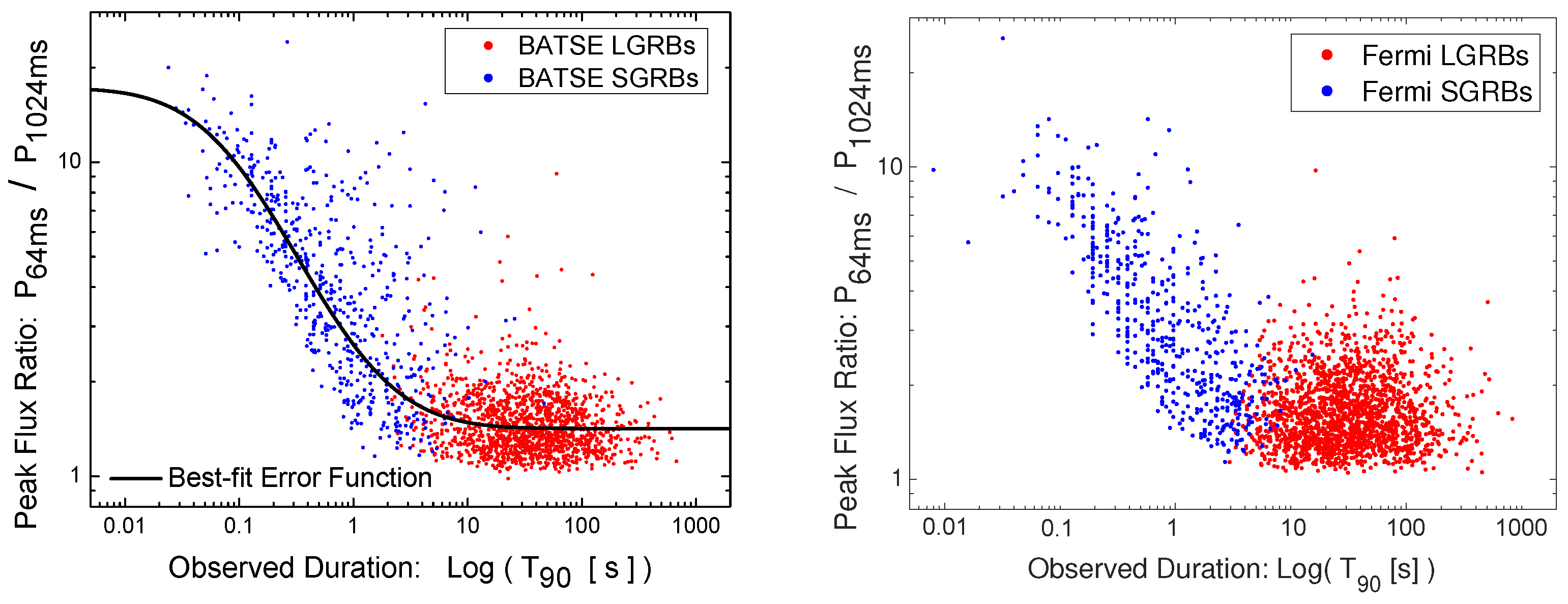
As an alternative, the effects of the gamma-ray detectors can be accounted for by modeling the detection threshold as part of the modeling of GRB properties [7,37]. For example, to remove the strong dependence of the detection threshold of Fermi-GBM on the timescale used for the definition of a GRB’s peak flux, we can define an effective timescale-free peak flux for all BATSE and Fermi GRBs. The existence of such an effective peak flux is noticeable in the plot of the ratio of GRB peak fluxes at different timescales as a function of their observed durations. Figure 3 illustrates the strong dependence of the peak flux ratios at 64 ms and 1024 ms timescales on the durations of GRBs measured by in the BATSE and Fermi catalogs. The two GRB classes are segregated via fuzzy classification methods [37,48,49] applied to and of the events in both catalogs [50]. We have already shown [7,37] the utility of this relationship in removing the effects of varying-timescale detector thresholds from the BATSE catalog. A similar procedure can be adopted for modeling the detection thresholds of Fermi-GBM and Swift-BAT gamma-ray detector thresholds. In the case of Fermi-GBM, the difference is minimal and amounts to only a wider range of triggering timescales ( s to s) compared to that of BATSE (64 ms to s). Furthermore, a realistic modeling of the detection threshold requires modeling the inherent fluctuations in the background gamma-ray photon counts as a Poisson process [22,37], leading to a fuzzy detection threshold at any given triggering timescale. This approach properly includes all GRBs in any catalog, down to the faintest events.
2.3. Model Calibration, Validation, and Selection
Once we implement the mathematical modeling approach described in Section 2.1 and the detection threshold model as laid out in Section 2.2, we can combine them to obtain probabilistic models for the observed rates of LGRBs and SGRBs in the given catalog of interest. The two LGRB and SGRB world models collectively yield the probability of observing the entire GRB catalog for a given set of input parameters. The most plausible parameters can be obtained by maximizing the likelihood of observing the catalog.
The last challenge lies in the maximization of the multivariate likelihood function resulting from the probabilistic models. This is due to the complex dependencies of the photon-counting detection mechanism of gamma-ray detectors in a limited energy window at different timescales on the intrinsic peak luminosity (), hardness (), duration (), and redshift (z) of each GRB. Notably, the BATSE LADs and Fermi-GBM have the nominal triggering energy window of 50–300 keV and trigger only on particular timescales, as noted previously. Furthermore, the intrinsic fuzziness of the detection threshold (due to background fluctuations) creates a nontrivial 5-dimensional fuzzy cut through the constructed probabilistic GRB world models. Thus, computing the probability of detection of GRBs for each input parameter set requires recomputing the probabilistic model’s normalization factor. In other words, calculating the likelihood of each parameter set of the models requires solving a 5-dimensional integration in the space of GRB properties and the gamma-ray detector characteristics.
Previous similar studies with the BATSE catalog data indicate that each computation of this multidimensional integral takes on the order of 100–1000 milliseconds [1,7,22,37]. The incorporation of data uncertainties in catalogs that are larger than BATSE catalog (such as Fermi-GBM) into this analysis via the Bayesian methods that we have detailed above will likely increase this computational cost by 1–2 orders of magnitude. As such, sampling the posterior probability density of the parameters of the GRB world models requires parallel Monte Carlo sampling algorithms. Existing software, such as ParaDRAM and ParaNest algorithms of the ParaMonte library [51,52,53,54] or MultiNest [55], are capable of distributing multiple simultaneous calculations of objective functions across a few processors in parallel.
In the presence of multiple competing GRB world models, the Bayesian probability theory offers a natural method of comparing and ranking multiple competing probabilistic world models for GRBs. This can be achieved by computing the plausibility of each model according to the Bayes rule. Consider, for example, the Bayesian problem of selecting the best model from a set of m competing models capable of describing all available data . For each model in the set, the posterior distribution of the parameters can be written as
where denotes the probability density function and represents the set of unknown parameters of the model . One can integrate the Bayes rule (Equation (1)) over the entire parameter space of the model and rearrange the equation to obtain
Equation (2) provides a method of computing the denominator of the Bayes rule in Equation (1), which, by definition, is the likelihood of observing data in a given model . It is sometimes called marginal likelihood since it is calculated by marginalizing the likelihood function over the entire parameter space of the model. However, more frequently, it is known as the Bayesian evidence or model evidence or simply the evidence. The utility of evidence goes beyond just serving as a normalizing constant in the Bayes rule, as it can be used for the calculation of Bayesian plausibility in yet another rewriting of the Bayes theorem, this time for the set of models :
Equation (3) gives the posterior probability density of the ith model in the set of all rival models , given the prior probability knowledge about model being correct. It is called the Bayesian plausibility, since it provides a measure of the plausibility of model assumptions in the light of available data and prior knowledge about the model. In the case of complete prior ignorance about all competing models, the Jaynes principle of maximum entropy [56] dictates the assignment of uniform equal prior probabilities to each of the competing models.
Despite the mathematical simplicity of Equation (3), its computation is frequently a challenging task. Nevertheless, the computation of Bayesian plausibility can be greatly simplified via analytical approximations to Equation (3) that are valid only under certain assumptions and asymptotic behaviors, such as in the limit of large datasets or when the posterior distribution of the parameters of the models can be well-approximated by a multivariate normal distribution. In such cases, approximate methods such as the Akaike Information Criterion (AIC) or the Bayesian Information Criterion (BIC) offer simple elegant solutions to model comparison [50,57]. In the special case of modeling GRB catalogs, however, the full numerical computation of the Bayesian plausibility for the competing models might be necessary. The aforementioned Monte Carlo sampling and integration tools can handle such intricate, computationally expensive numerical integrations.
3. Application to the BATSE Catalog of SGRBs
We now present an implementation of the Bayesian probabilistic approach to reconstructing the missing data (e.g., redshifts) of BATSE SGRBs.
3.1. Observational Data
We follow the same fuzzy clustering procedure applied to the BATSE catalog data as described in Shahmoradi and Nemiroff [7] to segregate SGRBs from LGRBs in the BATSE catalog. The resulting 565 SGRB sample that we obtain and use in this study is identical to that of Shahmoradi and Nemiroff [7]. Following Shahmoradi [37], Shahmoradi and Nemiroff [7], and Osborne et al. [1], we use the four observational prompt gamma-ray emission properties of SGRBs available in the BATSE catalog to constrain the population properties and the unknown redshifts of individual BATSE SGRBs (Figure 2).
3.2. Model Construction
The crucial step in modeling the population properties of BATSE SGRBs is to realize that one can use the existing prior knowledge about the overall cosmic redshift distribution of SGRBs to integrate over all possible redshifts for each observed SGRB in the BATSE catalog to infer a range of plausible values for the intrinsic properties of the corresponding SGRBs. These individually computed probability density functions (PDFs) of the intrinsic properties can be then used to infer the unknown parameters of the joint population distribution of the intrinsic properties of SGRBs.
Once the SGRB world model parameters are constrained, we can use the inferred population distribution of the intrinsic SGRB properties together with the observed properties to estimate the redshifts of individual BATSE SGRBs, independently of each other. The estimated redshifts can be again used to further constrain the intrinsic properties of SGRBs, which will then result in even tighter estimates for the individual redshifts of BATSE SGRBs. This recursive modeling can theoretically continue until convergence to a set of fixed individual redshift estimates occurs, although practical considerations frequently limit the procedure to only one cycle.
The lack of knowledge of the cosmic rate of SGRBs proves to be the largest source of uncertainty in SGRB population studies. At first glance, the above simple semi-Bayesian mathematical approach may sound like magic and perhaps, too good to be true. Sometimes it is. However, as explained in the previous sections, it can also lead to reasonably accurate results if some conditions regarding the problem and the observational dataset are satisfied.
Let represent the ith SGRB event in the BATSE catalog, with the four main SGRB prompt emission properties,
Here, the superscript is used to indicate that data are extracted exclusively from the light-curves of the events. These are essentially the values reported both in the BATSE catalog and in Shahmoradi and Nemiroff [58].
The entire BATSE dataset of 565 SGRB events attributes can then be represented as the collection of these events,
The peak brightness, , is included in our GRB world model as it, along with , determines the peak photon flux, , in the 50–300 keV range (the BATSE nominal detection energy window).
Given the available observed BATSE dataset, , the primary goal now is to constrain the probability density functions of the redshifts of individual BATSE SGRBs. To do this, the process of SGRB observation is modeled as a nonhomogeneous Poisson process whose mean rate parameter is the ‘observed’ cosmic SGRB rate, .
Each SGRB can be described as having the intrinsic properties
in the 5-dimensional attributes space, , of the 1024 ms isotropic peak luminosity (), the total isotropic emission (), the intrinsic spectral peak energy (), and the intrinsic duration (), as a function of the parameters, , of the observed SGRB rate model, . The probability of these SGRBs occurring with the given properties is then given by
where the term represents the BATSE-censored rate of SGRB occurrence in the universe. This can also be rewritten in terms of the intrinsic cosmic SGRB rate, , along with the BATSE detection efficiency function, , as
for a given set of input intrinsic SGRB attributes, , with as the set of the parameters of our models for the BATSE detection efficiency and the intrinsic cosmic SGRB rate, respectively. Assuming that there is no systematic evolution of SGRB characteristics with the redshift, the intrinsic SGRB rate itself can be written as
with , where is a statistical model, with denoting its parameters, that describes the population distribution of SGRBs in the 4-dimensional attributes space of , and the term represents the comoving rate density model of SGRBs with the set of parameters , while the factor in the denominator accounts for the cosmological time dilation. The comoving volume element per unit redshift, , is given by [59,60]
with and representing the dark matter and dark energy densities, respectively, and standing for the luminosity distance given by
where C represents the speed of light and represents the Hubble constant. The cosmological parameters in Equation (12) are set to , , and [61]. If the three rate models, , and their parameters were known a priori, one could readily compute the PDFs of the set of unknown redshifts of all BATSE SGRBs,
as
For a range of possible parameter values, the redshift probabilities can be computed by marginalizing over the entire parameter space, , of the model:
The problem, however, is that neither the rate models nor their parameters are known a priori. Even more problematic is the circular dependency of the posterior PDFs of and on each other:
To break this circular dependency, we can adopt the empirical Bayes approach described in Equation (2) to estimate the redshifts of BATSE SGRBs. First, we propose models for , whose parameters have yet to be constrained by observational data. Given the three rate models, we can then proceed to constrain the free parameters of the observed cosmic SGRB rate, , based on BATSE SGRB data.
The most appropriate fitting approach should take into account the observational uncertainties and any prior knowledge from independent sources. This can be achieved via the multilevel Bayesian methodology [22] by constructing the likelihood function and the posterior PDF of the parameters of the model while taking into account the uncertainties in observational data (see Equation (61) in [22]):
where Equation (17) holds under the assumptions of independent and identical distribution (i.e., the i.i.d. property) of BATSE SGRBs and there is no measurement uncertainty in the observational data, except redshift (z), which is completely unknown for BATSE SGRBs.
Once the posterior PDF of the model parameters is obtained, it can be plugged into Equation (15) to constrain the redshift PDF of individual BATSE SGRBs at the second level of modeling.
3.3. The SGRB Redshift Prior Knowledge
The main assumption in this work is that SGRBs are due to the coalescence of binary neutron stars or the merger of a neutron star and a black hole. It is widely believed that binary mergers require significant cosmological time to occur after the deaths of the parent stars and the formations of the neutron stars. In this scenario, the cosmic rate of SGRBs follows the Star Formation Rate (SFR) convolved with a distribution of the delay time between the formation of a binary system and its coalescence due to gravitational radiation.
There is currently no consensus on the statistical moments and shape of the distribution of the delay time between the deaths of supermassive stars and their subsequent coalescence to form SGRBs, solely based on observations of individual events and their host galaxies. The median delays vary widely in the range of ∼0.1–7 billion years, depending on the assumptions involved in estimation methods or in the dominant binary formation channels considered. Recent results from population synthesis simulations, however, favor very short delay times of a few hundred million years with long, negligible tails towards several billion years [7].
The extreme computational expenses imposed on this work by the complex mathematical models strongly limit the number of possible scenarios that could be considered for the cosmic rate of short GRBs. Thus, in order to approximate the comoving rate density of SGRBs, we adopt the Star Formation Rate (SFR) model, , described in [7] in the form of a piecewise power-law function,
with parameters
3.4. The SGRB Properties Rate Model:
As for the choice of the statistical model for the joint distribution of the four main intrinsic properties of SGRBs, , a multivariate log-normal distribution, , is assumed in this work, whose parameters (i.e., the mean vector and the covariance matrix), , will have to be constrained by data. The justification for the choice of a multivariate log-normal as the underlying intrinsic population distribution of SGRBs is multifolded. First, the observed joint distribution of BATSE SGRB properties highly resembles a log-normal shape [36] that is censored close to the detection threshold of BATSE. Second, unlike the power-law distribution which has traditionally been the default choice of model for the luminosity function of SGRBs, log-normal models provide natural upper and lower bounds on the total energy budget and luminosity of SGRBs, eliminating the need for setting artificial sharp bounds on the distributions to properly normalize them. Third, the log-normal and Gaussian distributions are among the most naturally occurring statistical distributions in nature, whose generalizations to multidimensions are also well-studied and understood. This is a highly desired property especially for our work, given the overall mathematical and computational complexity of the model proposed and developed here.
3.5. The BATSE Detection Threshold:
Compared to Fermi-GBM [63] and Swift-BAT [64], BATSE has a relatively simple triggering algorithm. The BATSE detection efficiency and algorithm have been already extensively studied by the BATSE team as well as independent authors [7,37,44,58]. However, the simple implementation and usage of the known BATSE trigger threshold for modeling the BATSE catalog’s sample incompleteness can lead to systematic biases in the inferred quantities of interest. Out of BATSE triggered on 2702 GRBs, only 2145, or approximately , have been consistently analyzed and reported in the current BATSE catalog, with the remaining either having a low accumulation of count rates or missing full spectral/temporal coverage [7]. Thus, the extent of sample incompleteness in the BATSE catalog is likely not fully and accurately represented by the BATSE triggering algorithm alone.
BATSE LADs generally triggered on a GRB if the number of photons per 64, 256, or 1024 ms arriving at the detectors in the 50–300 keV energy window, , reach a certain threshold in units of the background photon count fluctuations, . This threshold was typically set to 5.5 during much of BATSE’s operational lifetime. However, the naturally occurring fluctuations in the average background photon counts effectively lead to a monotonically increasing BATSE detection efficiency as a function of , instead of a sharp cutoff on the observed distribution of SGRBs.
Although the detection efficiency of most gamma-ray detectors depends solely on the observed peak photon flux in a limited energy window, the quantity of interest that is most often modeled and studied is the bolometric peak ‘energy’ flux (). This variable depends on the observed peak photon flux and the spectral peak energy () for the class of LGRBs [37] and also on the observed duration (e.g., ) of the burst for the class of SGRBs [7]. The effects of GRB duration on the peak flux measurement are very well illustrated in the left plot of Figure 3, where it is shown that for BATSE GRBs with 1024 ms, the timescale used for the definition of the peak flux does indeed matter. This is particularly important in modeling the triggering algorithm of BATSE Large Area Detectors when a short burst can be potentially detected on any of the three different peak flux timescales used in the triggering algorithm: 64 ms, 256 ms, and 1024 ms. Therefore, the detection modeling approach of Shahmoradi and Nemiroff [7] is adopted to construct a minimally biased model of BATSE trigger efficiency for the population study of short-hard bursts.
3.6. Results
Now, with a statistical model at hand for the observed rate of short GRBs, we proceed by first fitting the proposed censored cosmic SGRB rate model to 565 BATSE SGRB data under the redshift distribution scenario prescribed in the previous section. The posterior PDF of parameters of the cosmic rate model of SGRBs is explored by the Parallel Delayed-Rejection Adaptive Metropolis–Hastings Markov Chain Monte Carlo algorithm (the ParaDRAM algorithm) that is part of the larger Monte Carlo simulation package ParaMonte available in C, C++, Fortran, MATLAB, Python, and other programming languages available online (as of 31 March 2022) at https://github.com/cdslaborg/paramonte [52,53,65,66].
However, due to the complex truncation imposed on SGRB data and the world model by the BATSE detection threshold, the maximization of the posterior distribution of the parameters of the cosmic rate model of SGRBs is not only analytically intractable but also computationally extremely complex. Calculation of the posterior distribution as given by Equation (17) requires a multivariate integral over the four-dimensional space of SGRB variables at any given redshift. In addition, due to lack of redshift (z) information for BATSE SGRBs, the probability for the observation of each SGRB given the model parameters must be marginalized over all possible redshifts, adding another layer of integration to the four-dimensional integration. These numerical integrations make sampling from the posterior distribution of the parameters of the SGRB cosmic rate model an extremely difficult task. Therefore, the inclusion of the measurement uncertainties, which would make the computations far more complex, is not considered in this work.
The joint posterior distribution of the model parameters is then obtained by iterative sampling using a variant of Markov Chain Monte Carlo (MCMC) techniques known as Adaptive Metropolis–Hastings [67]. To further the efficiency of MCMC sampling, we implement all algorithms in Fortran [68,69] and approximate the numerical integration in the definition of the luminosity distance of Equation (12) by the analytical expressions of Wickramasinghe and Ukwatta [70]. This integration is encountered on the order of one billion times during the MCMC sampling of the posterior distribution.
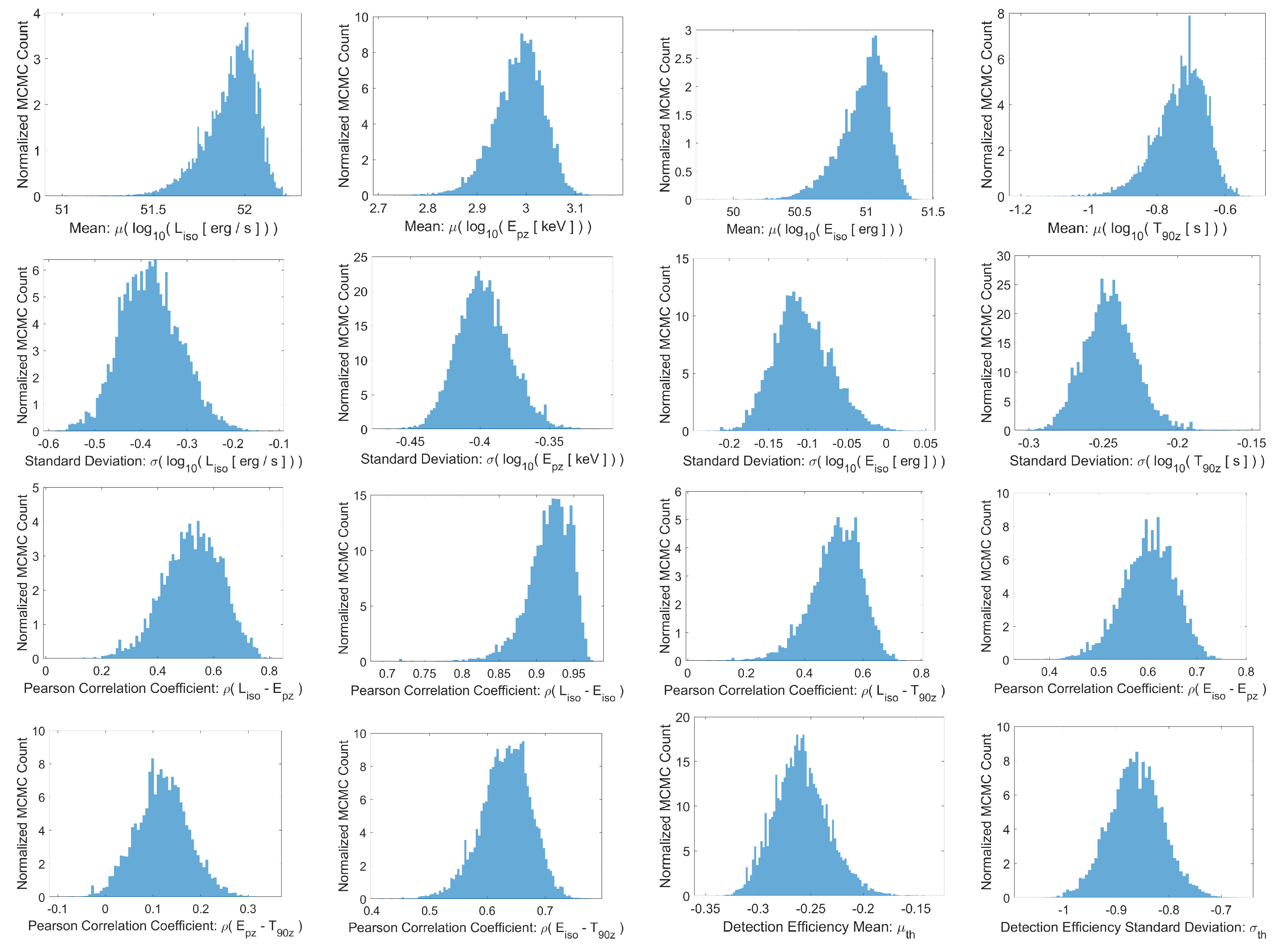
The computations were performed on 96 processors in parallel on two Skylake compute nodes of the Stampede 2 supercomputer at Texas Advanced Computing Center. We performed extensive tests to ensure a high level of accuracy of the high-dimensional numerical integrations involved in the derivation of the posterior distribution of the parameters of the censored cosmic rate model for SGRBs as given in Equation (17). The resulting best-fit parameters of the cosmic SGRB rate model are summarized in Table 1, and the marginal distributions of their parameters are compared with each other in Figure 4.
Once the parameters of the censored cosmic rate model Equation (9) are constrained, we use the calibrated model at the second level of the analysis to further constrain the PDFs of the unknown redshifts of individual BATSE SGRBs according to Equation (15). This iterative process can continue until convergence to a specific set of redshift PDFs occurs. However, given the computational complexity and the expense of each iteration, the iterative refinement process is stopped after obtaining the first round of estimates.
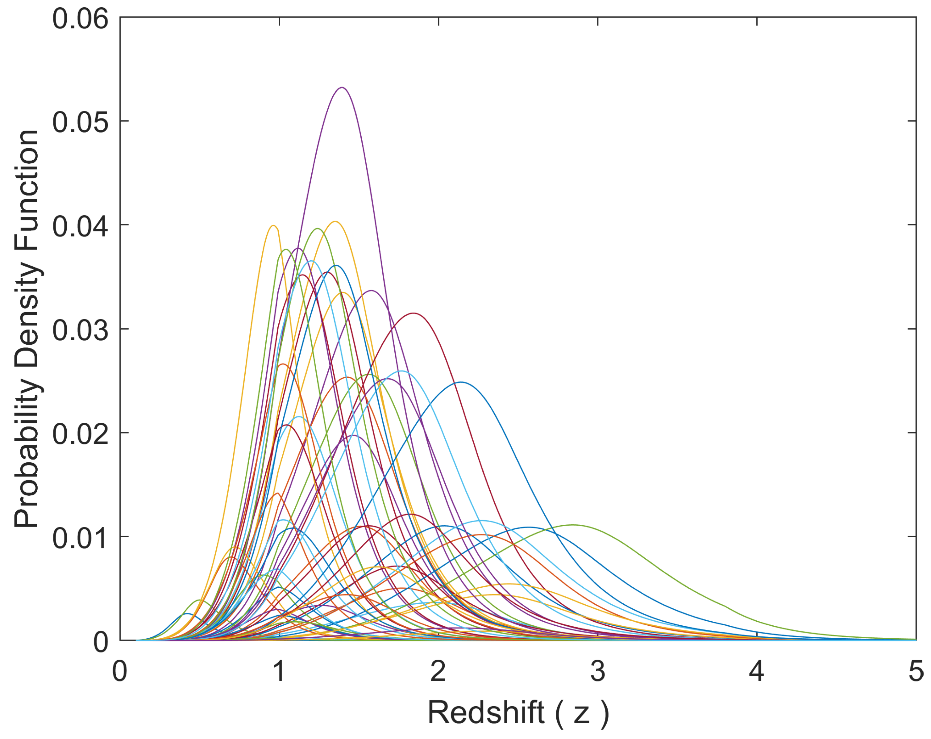
The mean redshifts together with and prediction intervals for the three rate density scenarios are also reported in Table 2. On average, the redshifts of individual BATSE SGRBs can be constrained to within a 50% uncertainty range of 0.51. At a 90% confidence level, the prediction intervals expand to wider a uncertainty range of 1.31. Figure 5 shows the derived probability density functions (PDFs) of a subset of 565 BATSE SGRBs. As illustrated, the redshifts of BATSE SGRBs are generally better constrained at lower redshifts.
4. Discussion and Concluding Remarks
In this work, a semi-Bayesian data-driven methodology was proposed to infer the unknown redshifts of 565 BATSE catalog SGRBs. Towards this, first, the two populations of BATSE LGRBs and SGRBs were segregated using the fuzzy C-means classification method based on the observed durations and spectral peak energies of 1966 BATSE GRBs with available spectral and temporal information. Then, the process of SGRB detection was modeled as a nonhomogeneous spatiotemporal Poisson process whose rate parameter was modeled by a multivariate log-normal distribution as a function of the four main SGRB intrinsic attributes: the 1024 ms isotropic peak luminosity (), the total isotropic emission (), the intrinsic spectral peak energy (), and the intrinsic duration (). To calibrate the parameters of the rate model, a fundamental assumption was made: SGRBs trace the Cosmic Star Formation Rate (SFR) convolved with a model for the binary neutron star merger delay distribution. Then, the resulting posterior probability densities of the model parameters were used to compute the probability density functions of the redshifts of individual BATSE SGRBs.
Although sample incompleteness may strongly affect an observational dataset, the proposed semi-Bayesian modeling framework enables us to overcome the limitations of the observational samples and missing data via reasonable prior distributions and appropriate modeling of the potential biases [71] present in observational data. The proposed methodology is different from and offers a parametric alternative to the existing nonparametric methods for quantifying the impact of missing data [72,73]. While generic and applicable to a wide range of research problems and datasets, this parametric probabilistic method requires certain assumptions to be met regarding the observational data to yield reasonably accurate unbiased constraints on the missing data. Most importantly, the effectiveness of the method correlates strongly and positively with the quality of data and the impact of the unknown components of data (e.g., redshift) on the known (observed) data. These two factors can together explain the significant difference between the tight constraints that Osborne et al. [1] obtain on the individual redshifts of BATSE LGRBs and the inferred redshifts of BATSE SGRBs in this work, as illustrated in Figure 5. We expect the Swift-BAT and particularly the Fermi-GBM catalogs to yield significantly tighter constraints on the unknown individual redshifts of Swift and Fermi LGRBs and SGRBs, due to the higher quality of data and the availability of redshift information for a significant number of events in these catalogs. This will ultimately lead to better independent estimates of the cosmic rates of LGRBs and SGRBs and their improved utilities in constraining the rate of GWR events. This will also enable the implementation of our proposed probabilistic framework for validating the inferred redshifts in these catalogs, an issue that remains untouched in present work due to the lack of any measured redshifts in the BATSE (SGRB) catalog. Nevertheless, Osborne et al. [1] show that our proposed methodology is capable of constraining the redshifts of GRBs in the presence of sufficient high-quality data.
Author Contributions
Conceptualization, A.S.; methodology, A.S. and F.B.; software, A.S., J.A.O. and F.B.; validation, A.S. and J.A.O.; formal analysis, A.S., J.A.O. and F.B.; investigation, A.S., J.A.O. and F.B.; resources, A.S.; data curation, A.S., J.A.O. and F.B.; writing—original draft preparation, A.S., J.A.O. and F.B.; writing—review and editing, A.S., J.A.O. and F.B.; visualization, A.S., J.A.O. and F.B.; supervision, A.S.; project administration, A.S.; funding acquisition, A.S. All authors have read and agreed to the published version of the manuscript.
Funding
This research received no external funding.
Institutional Review Board Statement
Not applicable.
Informed Consent Statement
Not applicable.
Data Availability Statement
Not applicable.
Conflicts of Interest
The authors declare no conflict of interest.
References
- Osborne, J.A.; Shahmoradi, A.; Nemiroff, R.J. A Multilevel Empirical Bayesian Approach to Estimating the Unknown Redshifts of 1366 BATSE Catalog Long-duration Gamma-Ray Bursts. APJ 2020, 903, 33. [Google Scholar] [CrossRef]
- Abbott, B.P.; Abbott, R.; Abbott, T.; Abernathy, M.; Acernese, F.; Ackley, K.; Adams, C.; Adams, T.; Addesso, P.; Adhikari, R.; et al. Observation of gravitational waves from a binary black hole merger. Phys. Rev. Lett. 2016, 116, 061102. [Google Scholar] [CrossRef] [PubMed]
- Abbott, B.P.; Abbott, R.; Abbott, T.; Acernese, F.; Ackley, K.; Adams, C.; Adams, T.; Addesso, P.; Adhikari, R.; Adya, V.; et al. GW170817: Observation of gravitational waves from a binary neutron star inspiral. Phys. Rev. Lett. 2017, 119, 161101. [Google Scholar] [CrossRef] [PubMed] [Green Version]
- Woosley, S.; Bloom, J. The supernova–gamma-ray burst connection. Annu. Rev. Astron. Astrophys. 2006, 44, 507–556. [Google Scholar] [CrossRef] [Green Version]
- Chen, H.Y.; Fishbach, M.; Holz, D.E. A two per cent Hubble constant measurement from standard sirens within five years. Nature 2018, 562, 545–547. [Google Scholar] [CrossRef] [Green Version]
- Kudryavtsev, M.; Svertilov, S.; Morozov, O. Observations of soft gamma-ray or hard X-ray bursts in the GRIF experiment on the Mir orbiting station. Astron. Lett. 2003, 29, 279–288. [Google Scholar] [CrossRef]
- Shahmoradi, A.; Nemiroff, R.J. Short versus long gamma-ray bursts: A comprehensive study of energetics and prompt gamma-ray correlations. Mon. Not. R. Astron. Soc. 2015, 451, 126–143. [Google Scholar] [CrossRef] [Green Version]
- Butler, N.R.; Bloom, J.S.; Poznanski, D. The cosmic rate, luminosity function, and intrinsic correlations of long gamma-ray bursts. APJ 2010, 711, 495. [Google Scholar] [CrossRef] [Green Version]
- Petrosian, V.; Kitanidis, E.; Kocevski, D. Cosmological evolution of long gamma-ray bursts and the star formation rate. APJ 2015, 806, 44. [Google Scholar] [CrossRef] [Green Version]
- Fenimore, E.E.; Ramirez-Ruiz, E. Redshifts for 220 batse gamma-ray bursts determined by variability and the cosmological consequences. arXiv 2000, arXiv:astro-ph/0004176. [Google Scholar]
- Reichart, D.E.; Lamb, D.Q.; Fenimore, E.E.; Ramirez-Ruiz, E.; Cline, T.L.; Hurley, K. A possible cepheid-like luminosity estimator for the long gamma-ray bursts. APJ 2001, 552, 57. [Google Scholar] [CrossRef] [Green Version]
- Band, D.L.; Norris, J.P.; Bonnell, J.T. Gamma-Ray Burst Intensity Distributions. APJ 2004, 613, 484. [Google Scholar] [CrossRef]
- Xiao, L.; Schaefer, B.E. Estimating redshifts for long gamma-ray bursts. APJ 2009, 707, 387. [Google Scholar] [CrossRef] [Green Version]
- Zhang, Q.G.; Wang, F. The formation rate of short gamma-ray bursts and gravitational waves. APJ 2017, 852, 1. [Google Scholar] [CrossRef] [Green Version]
- Zitouni, H.; Guessoum, N.; AlQassimi, K.M.; Alaryani, O. Distributions of pseudo-redshifts and durations (observed and intrinsic) of Fermi GRBs. Astrophys. Space Sci. 2018, 363, 223. [Google Scholar] [CrossRef] [Green Version]
- Guidorzi, C. Testing the gamma-ray burst variability/peak luminosity correlation using the pseudo-redshifts of a large sample of BATSE gamma-ray bursts. Mon. Not. R. Astron. Soc. 2005, 364, 163–168. [Google Scholar] [CrossRef] [Green Version]
- Ashcraft, T.; Schaefer, B.E. Are there any redshift > 8 gamma-ray bursts in the batse catalog? APJ 2007, 671, 1896. [Google Scholar] [CrossRef] [Green Version]
- Rizzuto, D.; Guidorzi, C.; Romano, P.; Covino, S.; Campana, S.; Capalbi, M.; Chincarini, G.; Cusumano, G.; Fugazza, D.; Mangano, V.; et al. Testing the gamma-ray burst variability/peak luminosity correlation on a Swift homogeneous sample. Mon. Not. R. Astron. Soc. 2007, 379, 619–628. [Google Scholar] [CrossRef] [Green Version]
- Bernardini, M.G.; Ghirlanda, G.; Campana, S.; Covino, S.; Salvaterra, R.; Atteia, J.-L.; Burlon, D.; Calderone, G.; D’Avanzo, P.; D’Elia, V.; et al. Comparing the spectral lag of short and long gamma-ray bursts and its relation with the luminosity. Mon. Not. R. Astron. Soc. 2014, 446, 1129–1138. [Google Scholar] [CrossRef] [Green Version]
- Poolakkil, S.; Preece, R.; Fletcher, C.; Goldstein, A.; Bhat, P.; Bissaldi, E.; Briggs, M.; Burns, E.; Cleveland, W.; Giles, M.; et al. The Fermi-GBM Gamma-Ray Burst spectral catalog: 10 yr of data. Astrophys. J. 2021, 913, 60. [Google Scholar] [CrossRef]
- Lien, A.; Sakamoto, T.; Barthelmy, S.D.; Baumgartner, W.H.; Cannizzo, J.K.; Chen, K.; Collins, N.R.; Cummings, J.R.; Gehrels, N.; Krimm, H.A.; et al. The third swift burst alert telescope gamma-ray burst catalog. Astrophys. J. 2016, 829, 7. [Google Scholar] [CrossRef] [Green Version]
- Shahmoradi, A. Multilevel Bayesian Parameter Estimation in the Presence of Model Inadequacy and Data Uncertainty. arXiv 2017, arXiv:1711.10599. [Google Scholar]
- Ripa, J. Statistical Analysis of the Observable Data of Gamma-Ray Bursts. arXiv 2011, arXiv:1105.2467. [Google Scholar]
- Madau, P.; Fragos, T. Radiation backgrounds at cosmic dawn: X-rays from compact binaries. APJ 2017, 840, 39. [Google Scholar] [CrossRef] [Green Version]
- Fermi-LAT Collaboration. A gamma-ray determination of the Universe’s star formation history. Science 2018, 362, 1031–1034. [Google Scholar] [CrossRef] [Green Version]
- Yu, H.; Wang, F.; Dai, Z.; Cheng, K. An unexpectedly low-redshift excess of Swift gamma-ray burst rate. APJ Suppl. Ser. 2015, 218, 13. [Google Scholar] [CrossRef] [Green Version]
- Lloyd-Ronning, N.M.; Aykutalp, A.; Johnson, J.L. On the cosmological evolution of long gamma-ray burst properties. Mon. Not. R. Astron. Soc. 2019, 488, 5823–5832. [Google Scholar] [CrossRef] [Green Version]
- Pescalli, A.; Ghirlanda, G.; Salvaterra, R.; Ghisellini, G.; Vergani, S.; Nappo, F.; Salafia, O.; Melandri, A.; Covino, S.; Götz, D. The rate and luminosity function of long gamma ray bursts. Astron. Astrophys. 2016, 587, A40. [Google Scholar] [CrossRef] [Green Version]
- Kistler, M.D.; Yüksel, H.; Beacom, J.F.; Hopkins, A.M.; Wyithe, J.S.B. The star formation rate in the reionization era as indicated by gamma-ray bursts. APJ Lett. 2009, 705, L104. [Google Scholar] [CrossRef] [Green Version]
- Belczynski, K.; Kalogera, V.; Rasio, F.A.; Taam, R.E.; Zezas, A.; Bulik, T.; Maccarone, T.J.; Ivanova, N. Compact object modeling with the StarTrack population synthesis code. APJ Suppl. Ser. 2008, 174, 223. [Google Scholar] [CrossRef]
- Belczynski, K.; Holz, D.E.; Bulik, T.; O’Shaughnessy, R. The first gravitational-wave source from the isolated evolution of two stars in the 40–100 solar mass range. Nature 2016, 534, 512–515. [Google Scholar] [CrossRef] [PubMed] [Green Version]
- Belczynski, K.; Askar, A.; Arca-Sedda, M.; Chruslinska, M.; Donnari, M.; Giersz, M.; Benacquista, M.; Spurzem, R.; Jin, D.; Wiktorowicz, G.; et al. The origin of the first neutron star–neutron star merger. Astron. Astrophys. 2018, 615, A91. [Google Scholar] [CrossRef]
- Compas, T.; Riley, J.; Agrawal, P.; Barrett, J.W.; Khandelwal, F.K.; Lau, M.Y.; Mandel, I.; de Mink, S.E.; Neijssel, C.; Riley, T.; et al. COMPAS: A rapid binary population synthesis suite. J. Open Source Softw. 2022, 7, 3838. [Google Scholar] [CrossRef]
- Breivik, K.; Coughlin, S.; Zevin, M.; Rodriguez, C.L.; Kremer, K.; Claire, S.Y.; Andrews, J.J.; Kurkowski, M.; Digman, M.C.; Larson, S.L.; et al. Cosmic variance in binary population synthesis. Astrophys. J. 2020, 898, 71. [Google Scholar] [CrossRef]
- Norris, J.P.; Gehrels, N. Constraints on high redshift GRBs from prompt emission. In GAMMA-RAY BURST: Sixth Huntsville Symposium; American Institute of Physics: New York, NY, USA, 2009. [Google Scholar]
- Balazs, L.G.; Bagoly, Z.; Horváth, I.; Mészáros, A.; Mészáros, P. On the difference between the short and long gamma-ray bursts. Astron. Astrophys. 2003, 401, 129–140. [Google Scholar] [CrossRef] [Green Version]
- Shahmoradi, A. A Multivariate Fit Luminosity Function and World Model for Long Gamma-Ray Bursts. APJ 2013, 766, 111. [Google Scholar] [CrossRef] [Green Version]
- Zhang, B.; Meszaros, P. Gamma-ray burst beaming: A universal configuration with a standard energy reservoir? APJ 2002, 571, 876. [Google Scholar] [CrossRef] [Green Version]
- Ghirlanda, G.; Ghisellini, G.; Lazzati, D. The collimation-corrected gamma-ray burst energies correlate with the peak energy of their νFν spectrum. APJ 2004, 616, 331. [Google Scholar] [CrossRef]
- Cenko, S.; Frail, D.; Harrison, F.; Kulkarni, S.; Nakar, E.; Chandra, P.; Butler, N.; Fox, D.; Gal-Yam, A.; Kasliwal, M.; et al. The collimation and energetics of the brightest Swift gamma-ray bursts. APJ 2010, 711, 641. [Google Scholar] [CrossRef] [Green Version]
- Gao, Y.; Dai, Z.G. GRB jet beaming angle statistics. Res. Astron. Astrophys. 2010, 10, 142. [Google Scholar] [CrossRef] [Green Version]
- Hayes, F.; Heng, I.S.; Veitch, J.; Williams, D. Comparing Short Gamma-Ray Burst Jet Structure Models. APJ 2020, 891, 124. [Google Scholar] [CrossRef]
- Shahmoradi, A.; Nemiroff, R.J. How Real detector thresholds create false standard candles. In AIP Conference Proceedings; American Institute of Physics: New York, NY, USA, 2009; Volume 1133, pp. 425–427. [Google Scholar]
- Shahmoradi, A.; Nemiroff, R.J. The possible impact of gamma-ray burst detector thresholds on cosmological standard candles. Mon. Not. R. Astron. Soc. 2011, 411, 1843–1856. [Google Scholar] [CrossRef] [Green Version]
- Fenimore, E.; Palmer, D.; Galassi, M.; Tavenner, T.; Barthelmy, S.; Gehrels, N.; Parsons, A.; Tueller, J. The Trigger Algorithm for the Burst Alert Telescope on Swift. In AIP Conference Proceedings; American Institute of Physics: New York, NY, USA, 2003; Volume 662, pp. 491–493. [Google Scholar]
- Ricker, G.; Atteia, J.L.; Crew, G.; Doty, J.; Fenimore, E.; Galassi, M.; Graziani, C.; Hurley, K.; Jernigan, J.; Kawai, N.; et al. The high energy transient explorer (HETE): Mission and science overview. In AIP Conference Proceedings; American Institute of Physics: New York, NY, USA, 2003; Volume 662, pp. 3–16. [Google Scholar]
- Bryant, C.M.; Osborne, J.A.; Shahmoradi, A. How unbiased statistical methods lead to biased scientific discoveries: A case study of the Efron–Petrosian statistic applied to the luminosity-redshift evolution of gamma-ray bursts. Mon. Not. R. Astron. Soc. 2021, 504, 4192–4203. [Google Scholar] [CrossRef]
- Rousseeuw, P.; Kaufman, L.; Trauwaert, E. Fuzzy clustering using scatter matrices. Comp. Stat. Data Anal. 1996, 23, 135–151. [Google Scholar] [CrossRef]
- Řípa, J.; Mészáros, A.; Wigger, C.; Huja, D.; Hudec, R.; Hajdas, W. Search for gamma-ray burst classes with the RHESSI satellite. Astron. Astrophys. 2009, 498, 399–406. [Google Scholar] [CrossRef] [Green Version]
- Tarnopolski, M. Analysis of the duration–hardness ratio plane of gamma-ray bursts using skewed distributions. Astrophys. J. 2019, 870, 105. [Google Scholar] [CrossRef]
- Shahmoradi, A.; Bagheri, F. ParaDRAM: A Cross-Language Toolbox for Parallel High-Performance Delayed-Rejection Adaptive Metropolis Markov Chain Monte Carlo Simulations. arXiv 2020, arXiv:2008.09589. [Google Scholar]
- Shahmoradi, A.; Bagheri, F. ParaMonte: A high-performance serial/parallel Monte Carlo simulation library for C, C++, Fortran. J. Open Source Softw. 2021, 6, 2741. [Google Scholar] [CrossRef]
- Shahmoradi, A. Gamma-Ray bursts: Energetics and Prompt Correlations. arXiv 2013, arXiv:1308.1097. [Google Scholar]
- Shahmoradi, A.; Bagheri, F.; Osborne, J.A. Fast fully-reproducible serial/parallel Monte Carlo and MCMC simulations and visualizations via ParaMonte::Python library. arXiv 2020, arXiv:2010.00724. [Google Scholar]
- Feroz, F.; Hobson, M.; Bridges, M. MultiNest: An efficient and robust Bayesian inference tool for cosmology and particle physics. Mon. Not. R. Astron. Soc. 2009, 398, 1601–1614. [Google Scholar] [CrossRef] [Green Version]
- Jaynes, E.T. Probability Theory: The Logic of Science; Cambridge University Press: Cambridge, UK, 2003. [Google Scholar]
- Tarnopolski, M. Analysis of the observed and intrinsic durations of Swift/BAT gamma-ray bursts. New Astron. 2016, 46, 54–59. [Google Scholar] [CrossRef] [Green Version]
- Shahmoradi, A.; Nemiroff, R.J. Hardness as a spectral peak estimator for gamma-ray bursts. Mon. Not. R. Astron. Soc. 2010, 407, 2075–2090. [Google Scholar] [CrossRef] [Green Version]
- Winberg, S. Gravitation and Cosmology; John Wiley & Sons: New York, NY, USA, 1972. [Google Scholar]
- Peebles, P.J.E. Principles of Physical Cosmology; Princeton University Press: Princeton, NJ, USA, 1993. [Google Scholar]
- Jarosik, N.; Bennett, C.; Dunkley, J.; Gold, B.; Greason, M.; Halpern, M.; Hill, R.; Hinshaw, G.; Kogut, A.; Komatsu, E.; et al. Seven-year wilkinson microwave anisotropy probe (WMAP*) observations: Sky maps, systematic errors, and basic results. Astrophys. J. Suppl. Ser. 2011, 192, 14. [Google Scholar] [CrossRef] [Green Version]
- Nakar, E. Short-hard gamma-ray bursts. Phys. Rep. 2007, 442, 166–236. [Google Scholar] [CrossRef] [Green Version]
- Meegan, C.; Lichti, G.; Bhat, P.; Bissaldi, E.; Briggs, M.S.; Connaughton, V.; Diehl, R.; Fishman, G.; Greiner, J.; Hoover, A.S.; et al. The Fermi gamma-ray burst monitor. Astrophys. J. 2009, 702, 791. [Google Scholar] [CrossRef] [Green Version]
- Gehrels, N.; Chincarini, G.; Giommi, P.; Mason, K.; Nousek, J.; Wells, A.; White, N.; Barthelmy, S.; Burrows, D.; Cominsky, L.; et al. The Swift gamma-ray burst mission. Astrophys. J. 2004, 611, 1005. [Google Scholar] [CrossRef] [Green Version]
- Shahmoradi, A. ParaMonte: A user-friendly parallel Monte Carlo optimization, sampling, and integration library for scientific inference. Bull. Am. Phys. Soc. 2019, 2019, G70.292. [Google Scholar]
- Kumbhare, S.; Shahmoradi, A. Parallel Adapative Monte Carlo Optimization, Sampling, and Integration in C/C++, Fortran, MATLAB, and Python. Bull. Am. Phys. Soc. 2020, 65, Y14.00005. [Google Scholar]
- Haario, H.; Saksman, E.; Tamminen, J. An adaptive Metropolis algorithm. Bernoulli 2001, 7, 223–242. [Google Scholar] [CrossRef] [Green Version]
- Backus, J. The history of Fortran I, II, and III. ACM Sigplan Not. 1978, 13, 165–180. [Google Scholar] [CrossRef]
- Metcalf, M.; Reid, J.; Cohen, M. Modern Fortran Explained; Oxford University Press: Oxford, UK, 2011. [Google Scholar]
- Wickramasinghe, T.; Ukwatta, T. An analytical approach for the determination of the luminosity distance in a flat universe with dark energy. Mon. Not. R. Astron. Soc. 2010, 406, 548–550. [Google Scholar] [CrossRef] [Green Version]
- Valore, P.; Dainotti, M.G.; Kopczyński, O. Ontological Categorizations and Selection Biases in Cosmology: The Case of Extra Galactic Objects. Found. Sci. 2021, 26, 515–529. [Google Scholar] [CrossRef]
- Dainotti, M.; Petrosian, V.; Willingale, R.; O’Brien, P.; Ostrowski, M.; Nagataki, S. Luminosity–time and luminosity–luminosity correlations for GRB prompt and afterglow plateau emissions. Mon. Not. R. Astron. Soc. 2015, 451, 3898–3908. [Google Scholar] [CrossRef] [Green Version]
- Dainotti, M.G.; Petrosian, V.; Bowden, L. Cosmological evolution of the formation rate of short gamma-ray bursts with and without extended emission. Astrophys. J. Lett. 2021, 914, L40. [Google Scholar] [CrossRef]
Figure 1.
A schematic illustration of the proposed probabilistic approach to inferring the unknown GRB redshifts of the Fermi, Swift, and other catalogs of GRBs. All axes are unitless.
Figure 1.
A schematic illustration of the proposed probabilistic approach to inferring the unknown GRB redshifts of the Fermi, Swift, and other catalogs of GRBs. All axes are unitless.

Figure 2.
An example time-resolved energy-resolved GRB light-curve illustrating the four main GRB properties that are commonly reported in GRB catalogs and used in this study to infer the missing redshift information of BATSE GRBs. The red, orange, green, and blue colored lines represent the aggregated energy flux received in each energy window as a function of time. The time in which it takes for the GRB to release 90% of its gamma-ray emissions in the observer frame is the . The violet- and gray-shaded curves represent the time-integrated spectrum and the energy-integrated (bolometric) light-curve of the GRB corresponding to the bolometric fluence of the GRB.

Figure 3.
An illustration of the similar effects of different triggering timescales on the detectability of GRBs in BATSE and Fermi catalogs: SGRBs are more detectable than LGRBs at shorter triggering timescales.
Figure 3.
An illustration of the similar effects of different triggering timescales on the detectability of GRBs in BATSE and Fermi catalogs: SGRBs are more detectable than LGRBs at shorter triggering timescales.

Figure 4.
The marginal posterior distributions of the 16 parameters of the SGRB world model.

Figure 5.
An illustration of the derived probability density functions (PDFs) of the individual redshifts of a subset of 565 BATSE SGRBs. Each curve corresponds to the inferred likelihood of different values of redshifts (z) for a single BATSE SGRB.
Figure 5.
An illustration of the derived probability density functions (PDFs) of the individual redshifts of a subset of 565 BATSE SGRBs. Each curve corresponds to the inferred likelihood of different values of redshifts (z) for a single BATSE SGRB.


Table 1.
Mean best-fit parameters of SGRB world model compared to LGRB world model of Shahmoradi [37].
Table 1.
Mean best-fit parameters of SGRB world model compared to LGRB world model of Shahmoradi [37].
| Parameter | SGRB World Model | LGRB World Model |
|---|---|---|
| Redshift Parameters (Equation (18)) | ||
| Log-normal Merger Delay (Equation (20)) | ||
| 0.1 | – | |
| 1.12 | – | |
| Location Parameters | ||
| Scale Parameters | ||
| Correlation Coefficients | ||
| BATSE Detection Efficiency | ||
Table 2.
BATSE 565 SGRB Redshift Estimates.
| Trigger | Mean (z) | Mode (z) | Q (z) | Q (z) | Q (z) | Q (z) | Q (z) |
|---|---|---|---|---|---|---|---|
| 108 | 1.62 | 1.58 | 1.05 | 1.35 | 1.58 | 1.85 | 2.30 |
| 138 | 1.50 | 1.47 | 0.99 | 1.26 | 1.48 | 1.71 | 2.12 |
| 185 | 1.08 | 1.02 | 0.70 | 0.91 | 1.06 | 1.23 | 1.54 |
| 207 | 0.77 | 0.75 | 0.50 | 0.64 | 0.76 | 0.88 | 1.09 |
| 218 | 1.89 | 1.86 | 1.24 | 1.59 | 1.86 | 2.15 | 2.64 |
| 229 | 1.39 | 1.36 | 0.92 | 1.17 | 1.36 | 1.58 | 1.95 |
| 254 | 1.22 | 1.17 | 0.83 | 1.03 | 1.19 | 1.37 | 1.70 |
| 289 | 0.84 | 0.83 | 0.54 | 0.70 | 0.83 | 0.96 | 1.18 |
| 297 | 1.04 | 0.99 | 0.70 | 0.89 | 1.02 | 1.17 | 1.43 |
| 373 | 1.34 | 1.30 | 0.89 | 1.12 | 1.31 | 1.52 | 1.89 |
| 432 | 0.56 | 0.53 | 0.35 | 0.46 | 0.55 | 0.65 | 0.82 |
| 474 | 0.46 | 0.43 | 0.29 | 0.37 | 0.44 | 0.52 | 0.67 |
| 480 | 0.56 | 0.53 | 0.36 | 0.46 | 0.55 | 0.64 | 0.82 |
| 486 | 1.21 | 1.16 | 0.80 | 1.02 | 1.18 | 1.38 | 1.71 |
| 491 | 1.18 | 1.13 | 0.78 | 0.99 | 1.15 | 1.35 | 1.68 |
| 508 | 1.49 | 1.45 | 0.98 | 1.24 | 1.46 | 1.69 | 2.10 |
| 512 | 0.69 | 0.66 | 0.43 | 0.57 | 0.67 | 0.79 | 0.99 |
| 537 | 1.65 | 1.61 | 1.09 | 1.39 | 1.62 | 1.88 | 2.33 |
| 547 | 1.02 | 0.99 | 0.69 | 0.87 | 1.00 | 1.15 | 1.41 |
| 551 | 0.77 | 0.75 | 0.50 | 0.65 | 0.76 | 0.88 | 1.09 |
| 555 | 1.22 | 1.16 | 0.81 | 1.02 | 1.18 | 1.38 | 1.72 |
| 568 | 0.80 | 0.79 | 0.53 | 0.68 | 0.79 | 0.92 | 1.13 |
| 575 | 0.97 | 0.98 | 0.65 | 0.83 | 0.96 | 1.10 | 1.35 |
| 603 | 0.84 | 0.83 | 0.55 | 0.71 | 0.83 | 0.96 | 1.18 |
| 677 | 0.48 | 0.46 | 0.30 | 0.40 | 0.47 | 0.56 | 0.71 |
| 729 | 0.87 | 0.86 | 0.56 | 0.73 | 0.86 | 0.99 | 1.22 |
| 734 | 1.32 | 1.27 | 0.88 | 1.11 | 1.29 | 1.51 | 1.87 |
| 788 | 1.11 | 1.04 | 0.73 | 0.93 | 1.08 | 1.25 | 1.57 |
| 799 | 0.93 | 0.93 | 0.59 | 0.78 | 0.92 | 1.06 | 1.33 |
| 809 | 1.01 | 0.99 | 0.67 | 0.86 | 0.99 | 1.13 | 1.40 |
| 830 | 0.68 | 0.66 | 0.44 | 0.57 | 0.67 | 0.78 | 0.98 |
| 834 | 2.48 | 2.47 | 1.61 | 2.09 | 2.45 | 2.83 | 3.46 |
| 836 | 1.37 | 1.34 | 0.90 | 1.15 | 1.34 | 1.55 | 1.92 |
| 845 | 2.05 | 2.02 | 1.34 | 1.72 | 2.02 | 2.33 | 2.88 |
| 856 | 1.18 | 1.13 | 0.78 | 0.99 | 1.15 | 1.35 | 1.68 |
| 867 | 1.65 | 1.60 | 1.08 | 1.38 | 1.61 | 1.88 | 2.34 |
| 878 | 1.05 | 0.99 | 0.70 | 0.89 | 1.03 | 1.18 | 1.46 |
| 906 | 1.06 | 1.00 | 0.72 | 0.90 | 1.04 | 1.19 | 1.47 |
| 909 | 2.89 | 2.89 | 1.90 | 2.44 | 2.85 | 3.30 | 3.96 |
| 929 | 1.59 | 1.56 | 1.05 | 1.34 | 1.56 | 1.81 | 2.23 |
| 936 | 0.91 | 0.91 | 0.61 | 0.78 | 0.90 | 1.03 | 1.27 |
| 942 | 2.36 | 2.34 | 1.54 | 1.99 | 2.33 | 2.69 | 3.31 |
| 974 | 2.76 | 2.76 | 1.82 | 2.33 | 2.73 | 3.15 | 3.79 |
| 1051 | 1.17 | 1.13 | 0.78 | 0.99 | 1.15 | 1.33 | 1.65 |
| 1073 | 1.10 | 1.04 | 0.74 | 0.93 | 1.08 | 1.24 | 1.53 |
| 1076 | 0.61 | 0.59 | 0.39 | 0.51 | 0.60 | 0.70 | 0.89 |
| 1088 | 0.47 | 0.44 | 0.30 | 0.39 | 0.46 | 0.54 | 0.69 |
| 1096 | 1.11 | 1.05 | 0.73 | 0.93 | 1.09 | 1.27 | 1.58 |
| 1097 | 0.97 | 0.98 | 0.64 | 0.83 | 0.96 | 1.10 | 1.36 |
| 1102 | 0.94 | 0.94 | 0.62 | 0.79 | 0.92 | 1.06 | 1.30 |
| 1112 | 1.40 | 1.36 | 0.93 | 1.18 | 1.37 | 1.58 | 1.95 |
| 1128 | 1.27 | 1.23 | 0.83 | 1.06 | 1.24 | 1.45 | 1.80 |
| 1129 | 1.79 | 1.78 | 1.17 | 1.51 | 1.76 | 2.04 | 2.52 |
| 1154 | 0.92 | 0.92 | 0.61 | 0.78 | 0.91 | 1.04 | 1.28 |
| 1211 | 1.21 | 1.17 | 0.81 | 1.02 | 1.19 | 1.37 | 1.70 |
| 1223 | 1.72 | 1.68 | 1.11 | 1.43 | 1.69 | 1.97 | 2.47 |
| 1289 | 1.23 | 1.18 | 0.83 | 1.03 | 1.20 | 1.39 | 1.72 |
| 1308 | 0.84 | 0.83 | 0.53 | 0.70 | 0.83 | 0.96 | 1.18 |
| 1346 | 1.63 | 1.59 | 1.07 | 1.36 | 1.60 | 1.86 | 2.30 |
| 1359 | 1.02 | 0.99 | 0.68 | 0.87 | 1.00 | 1.14 | 1.41 |
| 1404 | 1.90 | 1.88 | 1.24 | 1.60 | 1.87 | 2.17 | 2.67 |
| 1435 | 2.19 | 2.17 | 1.40 | 1.83 | 2.15 | 2.50 | 3.08 |
| 1443 | 1.32 | 1.24 | 0.87 | 1.09 | 1.28 | 1.50 | 1.89 |
| 1453 | 0.56 | 0.54 | 0.36 | 0.46 | 0.55 | 0.65 | 0.82 |
| 1461 | 0.93 | 0.92 | 0.61 | 0.78 | 0.91 | 1.05 | 1.30 |
| 1481 | 1.81 | 1.74 | 1.15 | 1.49 | 1.76 | 2.08 | 2.64 |
| 1518 | 1.16 | 1.11 | 0.79 | 0.98 | 1.13 | 1.31 | 1.62 |
| 1546 | 1.05 | 0.99 | 0.68 | 0.88 | 1.02 | 1.19 | 1.51 |
| 1553 | 0.71 | 0.68 | 0.46 | 0.59 | 0.69 | 0.81 | 1.01 |
| 1566 | 0.87 | 0.86 | 0.57 | 0.73 | 0.86 | 0.99 | 1.21 |
| 1588 | 0.91 | 0.91 | 0.61 | 0.78 | 0.90 | 1.03 | 1.27 |
| 1634 | 1.23 | 1.18 | 0.83 | 1.04 | 1.20 | 1.39 | 1.71 |
| 1635 | 1.14 | 1.09 | 0.76 | 0.96 | 1.11 | 1.29 | 1.59 |
| 1636 | 1.95 | 1.88 | 1.24 | 1.61 | 1.91 | 2.24 | 2.83 |
| 1637 | 1.80 | 1.78 | 1.15 | 1.51 | 1.77 | 2.06 | 2.56 |
| 1659 | 1.44 | 1.41 | 0.96 | 1.21 | 1.41 | 1.63 | 2.01 |
| 1662 | 1.13 | 1.08 | 0.75 | 0.96 | 1.10 | 1.27 | 1.57 |
| 1665 | 0.56 | 0.53 | 0.35 | 0.46 | 0.54 | 0.64 | 0.81 |
| 1679 | 3.51 | 3.69 | 2.38 | 3.03 | 3.50 | 3.94 | 4.72 |
| 1680 | 1.03 | 0.99 | 0.68 | 0.87 | 1.01 | 1.16 | 1.44 |
| 1683 | 1.36 | 1.27 | 0.88 | 1.11 | 1.31 | 1.55 | 1.99 |
| 1694 | 1.00 | 0.99 | 0.68 | 0.86 | 0.99 | 1.13 | 1.39 |
| 1719 | 1.00 | 0.99 | 0.67 | 0.85 | 0.98 | 1.12 | 1.38 |
| 1736 | 0.93 | 0.93 | 0.60 | 0.78 | 0.92 | 1.06 | 1.32 |
| 1741 | 0.83 | 0.82 | 0.54 | 0.70 | 0.82 | 0.95 | 1.17 |
| 1747 | 1.20 | 1.15 | 0.80 | 1.01 | 1.17 | 1.36 | 1.68 |
| 1760 | 0.94 | 0.93 | 0.63 | 0.80 | 0.92 | 1.06 | 1.30 |
| 1851 | 0.82 | 0.80 | 0.54 | 0.69 | 0.80 | 0.93 | 1.14 |
| 1953 | 1.36 | 1.32 | 0.92 | 1.15 | 1.34 | 1.54 | 1.91 |
| 1968 | 1.41 | 1.38 | 0.94 | 1.19 | 1.39 | 1.60 | 1.97 |
| 2003 | 1.10 | 1.05 | 0.74 | 0.94 | 1.08 | 1.25 | 1.54 |
| 2037 | 1.11 | 1.03 | 0.74 | 0.93 | 1.08 | 1.25 | 1.57 |
| 2040 | 1.65 | 1.62 | 1.09 | 1.39 | 1.62 | 1.88 | 2.31 |
| 2041 | 1.24 | 1.19 | 0.84 | 1.05 | 1.21 | 1.41 | 1.75 |
| 2043 | 1.51 | 1.48 | 0.99 | 1.26 | 1.48 | 1.72 | 2.12 |
| 2044 | 2.20 | 2.16 | 1.42 | 1.83 | 2.16 | 2.51 | 3.12 |
| 2049 | 0.84 | 0.82 | 0.55 | 0.71 | 0.83 | 0.95 | 1.17 |
| 2056 | 2.25 | 2.21 | 1.47 | 1.89 | 2.21 | 2.56 | 3.16 |
| 2068 | 0.55 | 0.52 | 0.34 | 0.45 | 0.53 | 0.63 | 0.81 |
| 2099 | 2.40 | 2.36 | 1.57 | 2.02 | 2.36 | 2.74 | 3.39 |
| 2103 | 1.31 | 1.27 | 0.88 | 1.10 | 1.28 | 1.48 | 1.82 |
| 2115 | 1.02 | 0.99 | 0.68 | 0.87 | 1.00 | 1.15 | 1.42 |
| 2117 | 1.04 | 0.99 | 0.69 | 0.88 | 1.02 | 1.17 | 1.45 |
| 2125 | 0.50 | 0.47 | 0.31 | 0.41 | 0.48 | 0.57 | 0.73 |
| 2126 | 0.91 | 0.90 | 0.60 | 0.77 | 0.90 | 1.03 | 1.26 |
| 2132 | 0.90 | 0.90 | 0.57 | 0.75 | 0.89 | 1.03 | 1.27 |
| 2142 | 1.86 | 1.82 | 1.21 | 1.56 | 1.82 | 2.12 | 2.62 |
| 2145 | 1.40 | 1.37 | 0.93 | 1.18 | 1.37 | 1.59 | 1.96 |
| 2146 | 0.99 | 0.99 | 0.66 | 0.84 | 0.98 | 1.12 | 1.37 |
| 2155 | 1.18 | 1.13 | 0.80 | 1.00 | 1.15 | 1.33 | 1.64 |
| 2159 | 1.14 | 1.07 | 0.73 | 0.95 | 1.11 | 1.30 | 1.63 |
| 2161 | 0.88 | 0.87 | 0.57 | 0.74 | 0.86 | 1.00 | 1.23 |
| 2163 | 1.46 | 1.43 | 0.97 | 1.23 | 1.43 | 1.66 | 2.04 |
| 2167 | 0.69 | 0.67 | 0.44 | 0.58 | 0.68 | 0.79 | 0.99 |
| 2201 | 1.11 | 1.07 | 0.75 | 0.95 | 1.09 | 1.26 | 1.54 |
| 2205 | 1.29 | 1.24 | 0.85 | 1.08 | 1.26 | 1.47 | 1.82 |
| 2206 | 1.10 | 1.05 | 0.74 | 0.94 | 1.08 | 1.24 | 1.52 |
| 2217 | 0.88 | 0.87 | 0.59 | 0.75 | 0.87 | 1.00 | 1.23 |
| 2220 | 1.09 | 1.04 | 0.73 | 0.93 | 1.07 | 1.23 | 1.51 |
| 2265 | 1.38 | 1.35 | 0.92 | 1.16 | 1.36 | 1.57 | 1.95 |
| 2268 | 1.49 | 1.43 | 0.98 | 1.24 | 1.45 | 1.70 | 2.13 |
| 2273 | 0.46 | 0.43 | 0.29 | 0.37 | 0.44 | 0.52 | 0.67 |
| 2283 | 1.20 | 1.14 | 0.79 | 1.01 | 1.17 | 1.37 | 1.72 |
| 2288 | 1.40 | 1.37 | 0.93 | 1.18 | 1.37 | 1.59 | 1.96 |
| 2312 | 1.07 | 1.01 | 0.72 | 0.91 | 1.05 | 1.21 | 1.48 |
| 2326 | 0.96 | 0.96 | 0.64 | 0.81 | 0.94 | 1.08 | 1.33 |
| 2327 | 2.78 | 2.79 | 1.84 | 2.36 | 2.76 | 3.17 | 3.81 |
| 2330 | 0.69 | 0.66 | 0.45 | 0.58 | 0.67 | 0.79 | 0.98 |
| 2332 | 0.96 | 0.97 | 0.63 | 0.81 | 0.95 | 1.09 | 1.35 |
| 2352 | 1.83 | 1.81 | 1.19 | 1.54 | 1.80 | 2.09 | 2.57 |
| 2353 | 1.52 | 1.50 | 1.01 | 1.28 | 1.50 | 1.73 | 2.13 |
| 2357 | 1.21 | 1.16 | 0.81 | 1.02 | 1.19 | 1.37 | 1.71 |
| 2358 | 1.40 | 1.36 | 0.91 | 1.16 | 1.37 | 1.59 | 1.98 |
| 2360 | 1.43 | 1.40 | 0.95 | 1.20 | 1.40 | 1.63 | 2.01 |
| 2365 | 1.71 | 1.68 | 1.12 | 1.44 | 1.68 | 1.95 | 2.41 |
| 2368 | 2.89 | 2.90 | 1.92 | 2.46 | 2.87 | 3.30 | 3.95 |
| 2372 | 1.15 | 1.11 | 0.77 | 0.98 | 1.13 | 1.31 | 1.61 |
| 2377 | 0.92 | 0.92 | 0.62 | 0.79 | 0.91 | 1.04 | 1.27 |
| 2382 | 3.11 | 3.15 | 2.06 | 2.65 | 3.09 | 3.54 | 4.21 |
| 2384 | 1.34 | 1.31 | 0.89 | 1.13 | 1.31 | 1.52 | 1.88 |
| 2395 | 1.00 | 0.99 | 0.65 | 0.84 | 0.98 | 1.13 | 1.39 |
| 2401 | 2.72 | 2.71 | 1.79 | 2.30 | 2.69 | 3.10 | 3.76 |
| 2424 | 2.62 | 2.60 | 1.72 | 2.21 | 2.59 | 2.99 | 3.64 |
| 2434 | 2.21 | 2.14 | 1.39 | 1.81 | 2.15 | 2.55 | 3.22 |
| 2448 | 1.52 | 1.49 | 1.00 | 1.28 | 1.49 | 1.73 | 2.13 |
| 2449 | 1.06 | 1.00 | 0.71 | 0.90 | 1.04 | 1.20 | 1.47 |
| 2454 | 2.24 | 2.20 | 1.45 | 1.87 | 2.20 | 2.55 | 3.17 |
| 2485 | 1.21 | 1.16 | 0.79 | 1.01 | 1.18 | 1.38 | 1.73 |
| 2487 | 1.01 | 0.99 | 0.68 | 0.86 | 0.99 | 1.13 | 1.39 |
| 2502 | 1.03 | 0.99 | 0.69 | 0.88 | 1.01 | 1.15 | 1.42 |
| 2504 | 0.87 | 0.86 | 0.57 | 0.73 | 0.85 | 0.99 | 1.21 |
| 2512 | 0.96 | 0.97 | 0.64 | 0.82 | 0.95 | 1.09 | 1.34 |
| 2513 | 2.10 | 2.07 | 1.38 | 1.77 | 2.06 | 2.39 | 2.95 |
| 2523 | 1.40 | 1.37 | 0.94 | 1.18 | 1.37 | 1.59 | 1.96 |
| 2529 | 1.76 | 1.70 | 1.11 | 1.45 | 1.72 | 2.02 | 2.55 |
| 2536 | 1.20 | 1.15 | 0.80 | 1.01 | 1.17 | 1.36 | 1.67 |
| 2564 | 1.33 | 1.29 | 0.89 | 1.12 | 1.31 | 1.51 | 1.87 |
| 2583 | 0.60 | 0.58 | 0.38 | 0.50 | 0.59 | 0.69 | 0.87 |
| 2585 | 1.94 | 1.88 | 1.23 | 1.60 | 1.90 | 2.23 | 2.80 |
| 2597 | 1.04 | 0.99 | 0.69 | 0.88 | 1.02 | 1.17 | 1.44 |
| 2599 | 0.81 | 0.79 | 0.52 | 0.67 | 0.79 | 0.92 | 1.14 |
| 2614 | 0.60 | 0.57 | 0.39 | 0.50 | 0.59 | 0.69 | 0.87 |
| 2615 | 0.83 | 0.82 | 0.53 | 0.70 | 0.82 | 0.95 | 1.17 |
| 2623 | 1.49 | 1.44 | 0.98 | 1.24 | 1.46 | 1.70 | 2.12 |
| 2632 | 1.58 | 1.52 | 1.03 | 1.31 | 1.54 | 1.81 | 2.27 |
| 2633 | 1.62 | 1.59 | 1.06 | 1.36 | 1.59 | 1.85 | 2.28 |
| 2649 | 1.03 | 0.99 | 0.68 | 0.88 | 1.01 | 1.16 | 1.44 |
| 2679 | 0.48 | 0.45 | 0.30 | 0.39 | 0.46 | 0.55 | 0.70 |
| 2680 | 2.69 | 2.65 | 1.76 | 2.26 | 2.64 | 3.07 | 3.74 |
| 2690 | 0.87 | 0.86 | 0.57 | 0.74 | 0.86 | 0.99 | 1.21 |
| 2693 | 1.26 | 1.23 | 0.84 | 1.06 | 1.24 | 1.44 | 1.78 |
| 2701 | 1.43 | 1.40 | 0.95 | 1.20 | 1.41 | 1.62 | 2.00 |
| 2715 | 0.54 | 0.51 | 0.34 | 0.45 | 0.53 | 0.62 | 0.79 |
| 2728 | 1.41 | 1.36 | 0.94 | 1.18 | 1.37 | 1.60 | 2.00 |
| 2748 | 1.20 | 1.15 | 0.79 | 1.01 | 1.17 | 1.36 | 1.69 |
| 2755 | 1.00 | 0.99 | 0.65 | 0.84 | 0.98 | 1.13 | 1.40 |
| 2757 | 1.30 | 1.25 | 0.86 | 1.09 | 1.27 | 1.48 | 1.86 |
| 2760 | 3.07 | 3.10 | 2.01 | 2.59 | 3.04 | 3.52 | 4.22 |
| 2776 | 2.02 | 2.00 | 1.31 | 1.70 | 1.99 | 2.30 | 2.83 |
| 2788 | 1.32 | 1.28 | 0.89 | 1.11 | 1.29 | 1.50 | 1.84 |
| 2795 | 0.87 | 0.85 | 0.57 | 0.73 | 0.85 | 0.98 | 1.21 |
| 2799 | 1.14 | 1.05 | 0.74 | 0.95 | 1.10 | 1.29 | 1.64 |
| 2800 | 1.45 | 1.41 | 0.96 | 1.22 | 1.42 | 1.64 | 2.02 |
| 2801 | 1.13 | 1.08 | 0.74 | 0.95 | 1.11 | 1.28 | 1.59 |
| 2810 | 2.51 | 2.47 | 1.64 | 2.10 | 2.47 | 2.87 | 3.52 |
| 2814 | 0.83 | 0.81 | 0.53 | 0.70 | 0.82 | 0.95 | 1.16 |
| 2821 | 1.12 | 1.07 | 0.74 | 0.95 | 1.10 | 1.27 | 1.58 |
| 2823 | 1.20 | 1.15 | 0.78 | 1.00 | 1.17 | 1.37 | 1.71 |
| 2828 | 1.44 | 1.41 | 0.96 | 1.21 | 1.42 | 1.64 | 2.02 |
| 2834 | 0.68 | 0.65 | 0.44 | 0.57 | 0.67 | 0.78 | 0.97 |
| 2844 | 1.95 | 1.92 | 1.26 | 1.63 | 1.92 | 2.23 | 2.76 |
| 2846 | 1.07 | 1.01 | 0.71 | 0.90 | 1.05 | 1.21 | 1.50 |
| 2849 | 2.16 | 2.10 | 1.38 | 1.79 | 2.11 | 2.48 | 3.11 |
| 2851 | 2.55 | 2.53 | 1.67 | 2.15 | 2.52 | 2.92 | 3.58 |
| 2860 | 1.30 | 1.25 | 0.88 | 1.09 | 1.27 | 1.47 | 1.82 |
| 2861 | 1.61 | 1.56 | 1.06 | 1.35 | 1.58 | 1.83 | 2.28 |
| 2873 | 1.04 | 0.99 | 0.68 | 0.88 | 1.03 | 1.18 | 1.47 |
| 2879 | 1.08 | 1.03 | 0.71 | 0.92 | 1.06 | 1.23 | 1.52 |
| 2892 | 1.03 | 0.99 | 0.67 | 0.87 | 1.01 | 1.16 | 1.45 |
| 2894 | 1.34 | 1.24 | 0.85 | 1.09 | 1.29 | 1.53 | 1.98 |
| 2910 | 0.95 | 0.95 | 0.62 | 0.80 | 0.93 | 1.08 | 1.33 |
| 2918 | 0.88 | 0.86 | 0.58 | 0.74 | 0.86 | 0.99 | 1.21 |
| 2933 | 0.63 | 0.61 | 0.41 | 0.53 | 0.62 | 0.73 | 0.92 |
| 2952 | 0.89 | 0.88 | 0.59 | 0.75 | 0.88 | 1.00 | 1.23 |
| 2964 | 1.14 | 1.09 | 0.75 | 0.96 | 1.12 | 1.30 | 1.61 |
| 2966 | 1.42 | 1.39 | 0.95 | 1.19 | 1.39 | 1.61 | 1.99 |
| 2973 | 1.21 | 1.17 | 0.81 | 1.03 | 1.19 | 1.37 | 1.70 |
| 2975 | 0.86 | 0.84 | 0.56 | 0.72 | 0.84 | 0.98 | 1.19 |
| 2977 | 1.09 | 1.03 | 0.73 | 0.93 | 1.07 | 1.22 | 1.51 |
| 2978 | 0.67 | 0.64 | 0.42 | 0.55 | 0.65 | 0.77 | 0.96 |
| 2987 | 1.32 | 1.28 | 0.89 | 1.11 | 1.29 | 1.50 | 1.84 |
| 2988 | 0.89 | 0.88 | 0.59 | 0.75 | 0.88 | 1.01 | 1.24 |
| 2995 | 0.83 | 0.81 | 0.54 | 0.70 | 0.82 | 0.95 | 1.16 |
| 3016 | 1.34 | 1.27 | 0.83 | 1.08 | 1.30 | 1.54 | 1.99 |
| 3027 | 0.75 | 0.72 | 0.48 | 0.62 | 0.73 | 0.86 | 1.06 |
| 3037 | 0.81 | 0.80 | 0.52 | 0.68 | 0.80 | 0.93 | 1.15 |
| 3038 | 1.19 | 1.15 | 0.81 | 1.01 | 1.17 | 1.35 | 1.66 |
| 3039 | 1.29 | 1.20 | 0.83 | 1.05 | 1.25 | 1.48 | 1.91 |
| 3043 | 1.22 | 1.15 | 0.79 | 1.01 | 1.18 | 1.39 | 1.76 |
| 3051 | 0.78 | 0.75 | 0.48 | 0.64 | 0.76 | 0.90 | 1.13 |
| 3066 | 0.95 | 0.95 | 0.63 | 0.81 | 0.94 | 1.07 | 1.31 |
| 3073 | 0.91 | 0.91 | 0.59 | 0.77 | 0.90 | 1.03 | 1.27 |
| 3078 | 0.88 | 0.87 | 0.58 | 0.75 | 0.87 | 1.00 | 1.23 |
| 3087 | 0.76 | 0.73 | 0.48 | 0.63 | 0.74 | 0.88 | 1.10 |
| 3094 | 1.15 | 1.10 | 0.77 | 0.97 | 1.12 | 1.29 | 1.59 |
| 3113 | 1.05 | 0.99 | 0.71 | 0.89 | 1.03 | 1.18 | 1.45 |
| 3114 | 1.80 | 1.78 | 1.17 | 1.51 | 1.78 | 2.06 | 2.53 |
| 3118 | 1.12 | 1.07 | 0.75 | 0.95 | 1.09 | 1.26 | 1.55 |
| 3121 | 1.43 | 1.40 | 0.96 | 1.21 | 1.41 | 1.63 | 2.00 |
| 3137 | 0.99 | 0.99 | 0.66 | 0.84 | 0.98 | 1.12 | 1.39 |
| 3144 | 3.51 | 3.69 | 2.37 | 3.03 | 3.49 | 3.94 | 4.71 |
| 3146 | 2.62 | 2.59 | 1.71 | 2.20 | 2.58 | 3.00 | 3.68 |
| 3152 | 0.55 | 0.52 | 0.35 | 0.45 | 0.54 | 0.63 | 0.81 |
| 3155 | 2.34 | 2.27 | 1.50 | 1.93 | 2.28 | 2.68 | 3.35 |
| 3160 | 2.05 | 2.02 | 1.34 | 1.73 | 2.02 | 2.34 | 2.88 |
| 3164 | 2.75 | 2.71 | 1.79 | 2.31 | 2.71 | 3.15 | 3.83 |
| 3173 | 0.48 | 0.46 | 0.30 | 0.40 | 0.47 | 0.55 | 0.70 |
| 3215 | 0.56 | 0.53 | 0.36 | 0.46 | 0.55 | 0.64 | 0.81 |
| 3218 | 0.75 | 0.73 | 0.48 | 0.62 | 0.74 | 0.86 | 1.07 |
| 3266 | 0.90 | 0.89 | 0.59 | 0.76 | 0.89 | 1.02 | 1.25 |
| 3278 | 1.81 | 1.79 | 1.18 | 1.52 | 1.78 | 2.07 | 2.55 |
| 3280 | 2.58 | 2.57 | 1.69 | 2.17 | 2.55 | 2.94 | 3.59 |
| 3282 | 0.78 | 0.76 | 0.50 | 0.65 | 0.77 | 0.90 | 1.10 |
| 3286 | 1.07 | 0.99 | 0.69 | 0.89 | 1.05 | 1.22 | 1.55 |
| 3293 | 1.11 | 1.05 | 0.74 | 0.94 | 1.08 | 1.25 | 1.54 |
| 3294 | 1.50 | 1.46 | 0.99 | 1.26 | 1.47 | 1.71 | 2.12 |
| 3297 | 0.85 | 0.83 | 0.56 | 0.72 | 0.84 | 0.96 | 1.18 |
| 3308 | 1.58 | 1.56 | 1.04 | 1.33 | 1.55 | 1.80 | 2.21 |
| 3323 | 1.13 | 1.09 | 0.77 | 0.96 | 1.11 | 1.28 | 1.58 |
| 3333 | 0.89 | 0.89 | 0.56 | 0.74 | 0.88 | 1.01 | 1.25 |
| 3335 | 1.76 | 1.74 | 1.15 | 1.48 | 1.73 | 2.01 | 2.47 |
| 3338 | 0.88 | 0.88 | 0.55 | 0.73 | 0.87 | 1.01 | 1.26 |
| 3340 | 1.15 | 1.10 | 0.78 | 0.98 | 1.13 | 1.30 | 1.60 |
| 3342 | 0.93 | 0.93 | 0.62 | 0.79 | 0.92 | 1.06 | 1.30 |
| 3349 | 0.97 | 0.98 | 0.64 | 0.83 | 0.96 | 1.10 | 1.35 |
| 3359 | 1.05 | 0.99 | 0.71 | 0.90 | 1.03 | 1.18 | 1.46 |
| 3374 | 1.22 | 1.18 | 0.82 | 1.03 | 1.19 | 1.38 | 1.70 |
| 3379 | 1.25 | 1.21 | 0.84 | 1.05 | 1.22 | 1.41 | 1.74 |
| 3384 | 0.84 | 0.83 | 0.52 | 0.69 | 0.83 | 0.96 | 1.19 |
| 3437 | 0.96 | 0.96 | 0.62 | 0.80 | 0.94 | 1.09 | 1.37 |
| 3441 | 1.00 | 0.99 | 0.66 | 0.85 | 0.99 | 1.13 | 1.40 |
| 3476 | 1.37 | 1.32 | 0.89 | 1.14 | 1.34 | 1.56 | 1.96 |
| 3477 | 1.72 | 1.70 | 1.13 | 1.45 | 1.69 | 1.96 | 2.41 |
| 3487 | 1.17 | 1.13 | 0.79 | 0.99 | 1.15 | 1.33 | 1.64 |
| 3494 | 1.38 | 1.34 | 0.92 | 1.16 | 1.35 | 1.56 | 1.93 |
| 3502 | 1.06 | 1.01 | 0.72 | 0.91 | 1.05 | 1.20 | 1.47 |
| 3510 | 1.05 | 0.99 | 0.70 | 0.89 | 1.03 | 1.19 | 1.47 |
| 3530 | 1.92 | 1.87 | 1.24 | 1.60 | 1.88 | 2.19 | 2.72 |
| 3545 | 1.44 | 1.41 | 0.96 | 1.21 | 1.41 | 1.63 | 2.02 |
| 3606 | 1.14 | 1.09 | 0.77 | 0.97 | 1.11 | 1.28 | 1.58 |
| 3611 | 2.80 | 2.77 | 1.83 | 2.35 | 2.76 | 3.20 | 3.88 |
| 3640 | 0.97 | 0.98 | 0.64 | 0.82 | 0.96 | 1.10 | 1.36 |
| 3642 | 0.79 | 0.77 | 0.52 | 0.67 | 0.78 | 0.90 | 1.11 |
| 3665 | 0.47 | 0.44 | 0.29 | 0.38 | 0.46 | 0.54 | 0.69 |
| 3668 | 0.78 | 0.76 | 0.51 | 0.65 | 0.77 | 0.89 | 1.10 |
| 3722 | 1.19 | 1.14 | 0.80 | 1.00 | 1.16 | 1.34 | 1.66 |
| 3728 | 1.18 | 1.14 | 0.79 | 1.00 | 1.16 | 1.34 | 1.66 |
| 3735 | 0.88 | 0.86 | 0.58 | 0.74 | 0.86 | 0.99 | 1.22 |
| 3737 | 0.79 | 0.77 | 0.51 | 0.66 | 0.77 | 0.90 | 1.10 |
| 3742 | 1.18 | 1.13 | 0.79 | 0.99 | 1.15 | 1.34 | 1.66 |
| 3751 | 1.08 | 1.03 | 0.74 | 0.93 | 1.07 | 1.22 | 1.50 |
| 3770 | 0.81 | 0.79 | 0.53 | 0.68 | 0.79 | 0.92 | 1.13 |
| 3774 | 1.08 | 1.01 | 0.70 | 0.90 | 1.05 | 1.22 | 1.53 |
| 3782 | 1.12 | 1.06 | 0.73 | 0.94 | 1.09 | 1.27 | 1.59 |
| 3791 | 0.88 | 0.86 | 0.58 | 0.74 | 0.86 | 0.99 | 1.21 |
| 3799 | 0.97 | 0.98 | 0.62 | 0.81 | 0.95 | 1.10 | 1.37 |
| 3810 | 0.83 | 0.81 | 0.54 | 0.70 | 0.82 | 0.95 | 1.16 |
| 3866 | 1.23 | 1.16 | 0.82 | 1.03 | 1.20 | 1.40 | 1.74 |
| 3867 | 1.04 | 0.99 | 0.71 | 0.89 | 1.02 | 1.17 | 1.44 |
| 3868 | 1.06 | 1.01 | 0.71 | 0.90 | 1.05 | 1.20 | 1.48 |
| 3888 | 0.95 | 0.95 | 0.64 | 0.81 | 0.93 | 1.07 | 1.31 |
| 3889 | 0.67 | 0.64 | 0.42 | 0.55 | 0.65 | 0.77 | 0.96 |
| 3894 | 1.27 | 1.23 | 0.85 | 1.07 | 1.24 | 1.44 | 1.78 |
| 3895 | 1.82 | 1.80 | 1.18 | 1.53 | 1.79 | 2.08 | 2.55 |
| 3902 | 0.58 | 0.56 | 0.37 | 0.48 | 0.57 | 0.67 | 0.84 |
| 3904 | 0.98 | 0.99 | 0.64 | 0.83 | 0.97 | 1.11 | 1.38 |
| 3910 | 0.90 | 0.89 | 0.56 | 0.75 | 0.89 | 1.03 | 1.30 |
| 3919 | 1.17 | 1.12 | 0.77 | 0.98 | 1.14 | 1.33 | 1.65 |
| 3921 | 0.86 | 0.85 | 0.57 | 0.73 | 0.85 | 0.98 | 1.19 |
| 3936 | 1.28 | 1.20 | 0.84 | 1.05 | 1.24 | 1.46 | 1.86 |
| 3939 | 1.88 | 1.81 | 1.20 | 1.55 | 1.83 | 2.16 | 2.74 |
| 3940 | 1.11 | 1.05 | 0.74 | 0.94 | 1.08 | 1.25 | 1.55 |
| 4327 | 0.52 | 0.49 | 0.32 | 0.42 | 0.50 | 0.60 | 0.76 |
| 4660 | 0.97 | 0.98 | 0.66 | 0.83 | 0.96 | 1.10 | 1.35 |
| 4744 | 0.95 | 0.96 | 0.63 | 0.81 | 0.94 | 1.08 | 1.33 |
| 4776 | 0.83 | 0.81 | 0.55 | 0.70 | 0.81 | 0.94 | 1.15 |
| 4807 | 0.86 | 0.84 | 0.55 | 0.72 | 0.84 | 0.98 | 1.21 |
| 4871 | 0.78 | 0.76 | 0.50 | 0.65 | 0.77 | 0.90 | 1.11 |
| 4955 | 0.80 | 0.78 | 0.53 | 0.68 | 0.79 | 0.92 | 1.12 |
| 5079 | 1.35 | 1.32 | 0.90 | 1.14 | 1.33 | 1.53 | 1.90 |
| 5206 | 0.84 | 0.83 | 0.55 | 0.71 | 0.83 | 0.96 | 1.17 |
| 5212 | 1.01 | 0.99 | 0.68 | 0.86 | 0.99 | 1.13 | 1.39 |
| 5277 | 0.70 | 0.68 | 0.46 | 0.59 | 0.69 | 0.80 | 1.00 |
| 5339 | 0.82 | 0.80 | 0.54 | 0.69 | 0.81 | 0.94 | 1.15 |
| 5439 | 0.66 | 0.63 | 0.42 | 0.55 | 0.64 | 0.76 | 0.96 |
| 5448 | 1.13 | 1.07 | 0.75 | 0.95 | 1.10 | 1.27 | 1.58 |
| 5453 | 1.63 | 1.61 | 1.07 | 1.37 | 1.60 | 1.86 | 2.29 |
| 5456 | 1.43 | 1.37 | 0.94 | 1.19 | 1.39 | 1.62 | 2.03 |
| 5458 | 0.89 | 0.88 | 0.53 | 0.73 | 0.88 | 1.03 | 1.33 |
| 5459 | 1.17 | 1.12 | 0.77 | 0.98 | 1.15 | 1.33 | 1.66 |
| 5461 | 1.44 | 1.41 | 0.96 | 1.21 | 1.41 | 1.64 | 2.02 |
| 5467 | 1.78 | 1.74 | 1.16 | 1.49 | 1.74 | 2.02 | 2.51 |
| 5469 | 1.13 | 1.07 | 0.76 | 0.96 | 1.10 | 1.27 | 1.56 |
| 5471 | 1.12 | 1.06 | 0.75 | 0.95 | 1.09 | 1.26 | 1.57 |
| 5485 | 2.63 | 2.62 | 1.73 | 2.22 | 2.59 | 3.00 | 3.65 |
| 5488 | 1.15 | 1.11 | 0.77 | 0.98 | 1.13 | 1.31 | 1.62 |
| 5491 | 1.01 | 0.99 | 0.65 | 0.85 | 0.99 | 1.14 | 1.42 |
| 5498 | 1.32 | 1.28 | 0.88 | 1.11 | 1.29 | 1.50 | 1.86 |
| 5499 | 1.32 | 1.28 | 0.89 | 1.11 | 1.29 | 1.50 | 1.84 |
| 5500 | 0.61 | 0.59 | 0.39 | 0.51 | 0.60 | 0.71 | 0.89 |
| 5501 | 1.21 | 1.16 | 0.80 | 1.02 | 1.18 | 1.38 | 1.72 |
| 5527 | 0.91 | 0.89 | 0.60 | 0.77 | 0.89 | 1.02 | 1.26 |
| 5528 | 1.13 | 1.08 | 0.77 | 0.96 | 1.11 | 1.27 | 1.57 |
| 5529 | 0.95 | 0.95 | 0.64 | 0.81 | 0.93 | 1.07 | 1.31 |
| 5533 | 0.85 | 0.83 | 0.56 | 0.72 | 0.84 | 0.96 | 1.18 |
| 5536 | 0.86 | 0.85 | 0.53 | 0.71 | 0.84 | 0.99 | 1.24 |
| 5537 | 1.40 | 1.37 | 0.94 | 1.18 | 1.38 | 1.59 | 1.96 |
| 5546 | 1.73 | 1.70 | 1.13 | 1.45 | 1.70 | 1.97 | 2.45 |
| 5547 | 1.23 | 1.18 | 0.83 | 1.04 | 1.20 | 1.39 | 1.71 |
| 5556 | 1.60 | 1.54 | 1.03 | 1.32 | 1.56 | 1.83 | 2.31 |
| 5560 | 1.27 | 1.23 | 0.85 | 1.07 | 1.24 | 1.44 | 1.78 |
| 5562 | 0.84 | 0.82 | 0.55 | 0.71 | 0.83 | 0.95 | 1.17 |
| 5564 | 0.59 | 0.56 | 0.37 | 0.49 | 0.58 | 0.68 | 0.86 |
| 5576 | 1.18 | 1.14 | 0.79 | 1.00 | 1.16 | 1.34 | 1.65 |
| 5592 | 1.07 | 1.02 | 0.71 | 0.91 | 1.05 | 1.21 | 1.50 |
| 5599 | 0.92 | 0.92 | 0.62 | 0.78 | 0.91 | 1.04 | 1.27 |
| 5607 | 0.92 | 0.91 | 0.62 | 0.78 | 0.90 | 1.04 | 1.27 |
| 5619 | 0.83 | 0.82 | 0.54 | 0.70 | 0.82 | 0.95 | 1.16 |
| 5620 | 0.88 | 0.87 | 0.55 | 0.73 | 0.86 | 1.01 | 1.26 |
| 5633 | 1.03 | 0.99 | 0.67 | 0.87 | 1.01 | 1.17 | 1.46 |
| 5638 | 1.66 | 1.64 | 1.09 | 1.40 | 1.64 | 1.90 | 2.33 |
| 5647 | 0.60 | 0.57 | 0.38 | 0.49 | 0.59 | 0.69 | 0.89 |
| 5650 | 1.45 | 1.41 | 0.96 | 1.21 | 1.42 | 1.64 | 2.03 |
| 5664 | 2.17 | 2.15 | 1.41 | 1.82 | 2.14 | 2.48 | 3.05 |
| 5724 | 1.20 | 1.15 | 0.81 | 1.02 | 1.18 | 1.36 | 1.67 |
| 5730 | 1.46 | 1.42 | 0.96 | 1.22 | 1.43 | 1.66 | 2.07 |
| 5733 | 1.04 | 0.99 | 0.68 | 0.88 | 1.01 | 1.17 | 1.45 |
| 5740 | 1.25 | 1.21 | 0.84 | 1.05 | 1.22 | 1.41 | 1.75 |
| 5770 | 1.32 | 1.28 | 0.89 | 1.11 | 1.29 | 1.49 | 1.83 |
| 5992 | 0.81 | 0.79 | 0.49 | 0.66 | 0.79 | 0.94 | 1.18 |
| 6091 | 1.42 | 1.34 | 0.91 | 1.16 | 1.37 | 1.63 | 2.09 |
| 6096 | 1.13 | 1.07 | 0.76 | 0.96 | 1.10 | 1.27 | 1.57 |
| 6105 | 0.99 | 0.99 | 0.66 | 0.84 | 0.98 | 1.12 | 1.38 |
| 6117 | 1.38 | 1.35 | 0.93 | 1.17 | 1.36 | 1.57 | 1.93 |
| 6120 | 1.00 | 0.99 | 0.67 | 0.85 | 0.98 | 1.13 | 1.38 |
| 6123 | 0.49 | 0.46 | 0.31 | 0.41 | 0.48 | 0.56 | 0.72 |
| 6135 | 2.12 | 2.09 | 1.38 | 1.78 | 2.08 | 2.41 | 2.98 |
| 6136 | 1.20 | 1.12 | 0.79 | 1.00 | 1.16 | 1.36 | 1.71 |
| 6145 | 1.07 | 1.01 | 0.72 | 0.91 | 1.05 | 1.20 | 1.48 |
| 6153 | 1.35 | 1.32 | 0.90 | 1.14 | 1.33 | 1.53 | 1.90 |
| 6166 | 0.91 | 0.91 | 0.59 | 0.76 | 0.89 | 1.03 | 1.27 |
| 6178 | 1.60 | 1.57 | 1.05 | 1.35 | 1.57 | 1.82 | 2.24 |
| 6180 | 1.43 | 1.40 | 0.95 | 1.20 | 1.41 | 1.63 | 2.02 |
| 6182 | 0.99 | 0.99 | 0.66 | 0.84 | 0.97 | 1.12 | 1.39 |
| 6204 | 0.97 | 0.97 | 0.63 | 0.81 | 0.95 | 1.10 | 1.37 |
| 6205 | 0.97 | 0.98 | 0.64 | 0.82 | 0.96 | 1.10 | 1.37 |
| 6215 | 1.01 | 0.99 | 0.68 | 0.86 | 0.99 | 1.14 | 1.41 |
| 6216 | 1.48 | 1.39 | 0.95 | 1.21 | 1.43 | 1.70 | 2.18 |
| 6219 | 0.94 | 0.93 | 0.60 | 0.78 | 0.92 | 1.07 | 1.36 |
| 6230 | 0.78 | 0.75 | 0.50 | 0.65 | 0.76 | 0.89 | 1.10 |
| 6237 | 1.15 | 1.11 | 0.77 | 0.98 | 1.13 | 1.31 | 1.61 |
| 6238 | 1.17 | 1.12 | 0.78 | 0.99 | 1.15 | 1.33 | 1.65 |
| 6251 | 1.09 | 1.02 | 0.73 | 0.92 | 1.07 | 1.24 | 1.54 |
| 6263 | 0.82 | 0.79 | 0.52 | 0.68 | 0.81 | 0.95 | 1.19 |
| 6265 | 0.74 | 0.72 | 0.48 | 0.62 | 0.73 | 0.85 | 1.05 |
| 6275 | 1.18 | 1.13 | 0.79 | 1.00 | 1.15 | 1.33 | 1.65 |
| 6281 | 1.42 | 1.38 | 0.92 | 1.18 | 1.39 | 1.62 | 2.03 |
| 6284 | 1.18 | 1.14 | 0.79 | 1.00 | 1.16 | 1.34 | 1.65 |
| 6292 | 1.18 | 1.12 | 0.78 | 0.99 | 1.15 | 1.34 | 1.68 |
| 6299 | 0.93 | 0.92 | 0.60 | 0.78 | 0.91 | 1.05 | 1.31 |
| 6301 | 1.55 | 1.51 | 1.03 | 1.30 | 1.51 | 1.75 | 2.16 |
| 6307 | 1.30 | 1.26 | 0.87 | 1.09 | 1.27 | 1.47 | 1.81 |
| 6314 | 2.15 | 2.11 | 1.40 | 1.80 | 2.11 | 2.46 | 3.06 |
| 6331 | 1.99 | 1.94 | 1.28 | 1.66 | 1.95 | 2.28 | 2.85 |
| 6338 | 0.99 | 0.99 | 0.65 | 0.84 | 0.97 | 1.12 | 1.39 |
| 6341 | 1.20 | 1.15 | 0.81 | 1.02 | 1.18 | 1.36 | 1.68 |
| 6342 | 1.02 | 0.99 | 0.65 | 0.85 | 0.99 | 1.16 | 1.49 |
| 6343 | 1.02 | 0.99 | 0.66 | 0.86 | 1.00 | 1.15 | 1.44 |
| 6347 | 1.20 | 1.15 | 0.80 | 1.01 | 1.17 | 1.36 | 1.68 |
| 6354 | 0.67 | 0.64 | 0.42 | 0.55 | 0.66 | 0.78 | 0.98 |
| 6361 | 0.96 | 0.96 | 0.64 | 0.81 | 0.95 | 1.09 | 1.35 |
| 6368 | 0.69 | 0.66 | 0.45 | 0.58 | 0.68 | 0.79 | 0.98 |
| 6372 | 1.18 | 1.14 | 0.79 | 1.00 | 1.16 | 1.34 | 1.65 |
| 6376 | 1.06 | 1.00 | 0.71 | 0.90 | 1.04 | 1.20 | 1.48 |
| 6385 | 1.09 | 1.03 | 0.73 | 0.93 | 1.07 | 1.23 | 1.51 |
| 6386 | 1.22 | 1.18 | 0.83 | 1.03 | 1.19 | 1.37 | 1.70 |
| 6398 | 1.54 | 1.50 | 0.99 | 1.28 | 1.51 | 1.76 | 2.20 |
| 6401 | 2.01 | 1.98 | 1.31 | 1.69 | 1.97 | 2.29 | 2.82 |
| 6411 | 1.44 | 1.41 | 0.94 | 1.20 | 1.41 | 1.65 | 2.06 |
| 6412 | 1.27 | 1.23 | 0.84 | 1.07 | 1.24 | 1.45 | 1.81 |
| 6427 | 1.08 | 1.02 | 0.72 | 0.92 | 1.06 | 1.22 | 1.51 |
| 6436 | 0.61 | 0.58 | 0.39 | 0.50 | 0.60 | 0.71 | 0.90 |
| 6439 | 1.20 | 1.16 | 0.80 | 1.01 | 1.18 | 1.36 | 1.69 |
| 6443 | 1.36 | 1.32 | 0.90 | 1.14 | 1.33 | 1.55 | 1.93 |
| 6445 | 1.28 | 1.24 | 0.86 | 1.08 | 1.26 | 1.45 | 1.80 |
| 6447 | 1.22 | 1.18 | 0.81 | 1.02 | 1.19 | 1.38 | 1.72 |
| 6452 | 1.36 | 1.32 | 0.90 | 1.13 | 1.33 | 1.54 | 1.91 |
| 6462 | 0.92 | 0.92 | 0.61 | 0.78 | 0.90 | 1.04 | 1.27 |
| 6469 | 1.00 | 0.99 | 0.66 | 0.85 | 0.99 | 1.14 | 1.41 |
| 6486 | 0.63 | 0.60 | 0.39 | 0.51 | 0.61 | 0.72 | 0.92 |
| 6488 | 2.31 | 2.29 | 1.51 | 1.95 | 2.28 | 2.63 | 3.23 |
| 6497 | 2.54 | 2.53 | 1.66 | 2.15 | 2.51 | 2.90 | 3.52 |
| 6535 | 0.83 | 0.80 | 0.54 | 0.70 | 0.81 | 0.95 | 1.17 |
| 6540 | 0.80 | 0.79 | 0.50 | 0.67 | 0.79 | 0.92 | 1.14 |
| 6542 | 0.98 | 0.99 | 0.65 | 0.84 | 0.96 | 1.11 | 1.36 |
| 6543 | 0.81 | 0.77 | 0.51 | 0.67 | 0.79 | 0.93 | 1.18 |
| 6547 | 1.02 | 0.99 | 0.68 | 0.87 | 1.00 | 1.15 | 1.42 |
| 6562 | 1.33 | 1.29 | 0.88 | 1.11 | 1.30 | 1.51 | 1.89 |
| 6569 | 1.32 | 1.27 | 0.87 | 1.10 | 1.29 | 1.51 | 1.88 |
| 6571 | 1.13 | 1.07 | 0.74 | 0.95 | 1.10 | 1.28 | 1.59 |
| 6573 | 1.03 | 0.99 | 0.69 | 0.88 | 1.01 | 1.16 | 1.43 |
| 6579 | 1.36 | 1.31 | 0.91 | 1.14 | 1.33 | 1.54 | 1.91 |
| 6580 | 1.32 | 1.27 | 0.89 | 1.11 | 1.29 | 1.50 | 1.86 |
| 6586 | 1.36 | 1.30 | 0.88 | 1.12 | 1.32 | 1.55 | 1.96 |
| 6591 | 1.33 | 1.29 | 0.90 | 1.12 | 1.30 | 1.51 | 1.86 |
| 6606 | 0.80 | 0.78 | 0.52 | 0.67 | 0.78 | 0.91 | 1.11 |
| 6634 | 1.94 | 1.90 | 1.25 | 1.62 | 1.90 | 2.23 | 2.78 |
| 6635 | 0.87 | 0.83 | 0.54 | 0.71 | 0.84 | 0.99 | 1.27 |
| 6638 | 1.40 | 1.36 | 0.94 | 1.18 | 1.37 | 1.59 | 1.97 |
| 6641 | 1.34 | 1.30 | 0.90 | 1.13 | 1.31 | 1.52 | 1.90 |
| 6643 | 0.92 | 0.91 | 0.60 | 0.77 | 0.90 | 1.04 | 1.27 |
| 6645 | 0.81 | 0.79 | 0.52 | 0.68 | 0.80 | 0.93 | 1.15 |
| 6659 | 1.09 | 1.02 | 0.73 | 0.92 | 1.06 | 1.23 | 1.53 |
| 6662 | 2.42 | 2.39 | 1.59 | 2.04 | 2.39 | 2.76 | 3.39 |
| 6671 | 0.67 | 0.64 | 0.43 | 0.56 | 0.66 | 0.77 | 0.96 |
| 6679 | 0.75 | 0.73 | 0.49 | 0.63 | 0.74 | 0.86 | 1.06 |
| 6682 | 1.05 | 1.00 | 0.70 | 0.90 | 1.03 | 1.19 | 1.47 |
| 6689 | 0.98 | 0.98 | 0.65 | 0.83 | 0.96 | 1.10 | 1.36 |
| 6693 | 1.07 | 1.02 | 0.72 | 0.91 | 1.05 | 1.21 | 1.49 |
| 6697 | 1.37 | 1.33 | 0.92 | 1.15 | 1.34 | 1.55 | 1.92 |
| 6700 | 0.71 | 0.68 | 0.46 | 0.59 | 0.70 | 0.81 | 1.01 |
| 6710 | 1.75 | 1.73 | 1.14 | 1.47 | 1.72 | 1.99 | 2.45 |
| 6715 | 0.97 | 0.97 | 0.65 | 0.83 | 0.95 | 1.09 | 1.34 |
| 6718 | 1.24 | 1.18 | 0.81 | 1.03 | 1.21 | 1.41 | 1.78 |
| 6753 | 2.66 | 2.64 | 1.74 | 2.24 | 2.62 | 3.04 | 3.71 |
| 6757 | 2.04 | 2.00 | 1.33 | 1.71 | 2.00 | 2.32 | 2.87 |
| 6786 | 1.28 | 1.24 | 0.85 | 1.08 | 1.26 | 1.46 | 1.81 |
| 6787 | 0.93 | 0.92 | 0.61 | 0.79 | 0.91 | 1.05 | 1.28 |
| 6788 | 0.38 | 0.36 | 0.24 | 0.31 | 0.37 | 0.44 | 0.56 |
| 6800 | 0.67 | 0.64 | 0.43 | 0.55 | 0.65 | 0.77 | 0.96 |
| 6824 | 1.06 | 0.99 | 0.71 | 0.90 | 1.03 | 1.19 | 1.49 |
| 6866 | 1.18 | 1.13 | 0.78 | 0.99 | 1.15 | 1.33 | 1.65 |
| 6867 | 1.63 | 1.58 | 1.04 | 1.35 | 1.59 | 1.87 | 2.35 |
| 6870 | 1.75 | 1.71 | 1.12 | 1.45 | 1.71 | 2.00 | 2.49 |
| 6904 | 0.36 | 0.33 | 0.22 | 0.29 | 0.35 | 0.41 | 0.54 |
| 6916 | 0.71 | 0.68 | 0.46 | 0.59 | 0.69 | 0.81 | 1.01 |
| 6931 | 0.70 | 0.68 | 0.46 | 0.59 | 0.69 | 0.80 | 0.99 |
| 7009 | 0.44 | 0.42 | 0.28 | 0.36 | 0.43 | 0.51 | 0.65 |
| 7060 | 0.80 | 0.78 | 0.52 | 0.67 | 0.79 | 0.92 | 1.13 |
| 7063 | 0.40 | 0.38 | 0.25 | 0.33 | 0.39 | 0.46 | 0.60 |
| 7078 | 0.77 | 0.75 | 0.49 | 0.64 | 0.75 | 0.88 | 1.09 |
| 7102 | 1.03 | 0.99 | 0.69 | 0.88 | 1.01 | 1.16 | 1.42 |
| 7106 | 1.16 | 1.11 | 0.78 | 0.98 | 1.13 | 1.31 | 1.61 |
| 7133 | 1.11 | 1.05 | 0.75 | 0.95 | 1.09 | 1.25 | 1.55 |
| 7142 | 0.92 | 0.91 | 0.62 | 0.78 | 0.90 | 1.04 | 1.27 |
| 7148 | 1.52 | 1.49 | 1.00 | 1.27 | 1.49 | 1.73 | 2.13 |
| 7159 | 1.09 | 1.00 | 0.69 | 0.90 | 1.06 | 1.25 | 1.60 |
| 7173 | 1.01 | 0.99 | 0.68 | 0.86 | 0.99 | 1.13 | 1.40 |
| 7187 | 0.75 | 0.73 | 0.48 | 0.63 | 0.74 | 0.86 | 1.08 |
| 7227 | 0.97 | 0.98 | 0.64 | 0.82 | 0.95 | 1.09 | 1.35 |
| 7240 | 0.77 | 0.74 | 0.50 | 0.64 | 0.75 | 0.88 | 1.09 |
| 7281 | 0.76 | 0.73 | 0.48 | 0.63 | 0.75 | 0.88 | 1.11 |
| 7283 | 1.27 | 1.23 | 0.86 | 1.07 | 1.24 | 1.43 | 1.76 |
| 7287 | 0.65 | 0.61 | 0.41 | 0.53 | 0.63 | 0.75 | 0.96 |
| 7290 | 1.05 | 0.99 | 0.70 | 0.89 | 1.03 | 1.19 | 1.48 |
| 7292 | 0.87 | 0.86 | 0.57 | 0.74 | 0.86 | 0.99 | 1.21 |
| 7294 | 0.76 | 0.73 | 0.49 | 0.63 | 0.74 | 0.86 | 1.07 |
| 7297 | 1.54 | 1.51 | 1.02 | 1.30 | 1.51 | 1.75 | 2.16 |
| 7305 | 0.59 | 0.56 | 0.38 | 0.49 | 0.58 | 0.68 | 0.86 |
| 7329 | 1.23 | 1.17 | 0.83 | 1.03 | 1.20 | 1.39 | 1.73 |
| 7344 | 0.91 | 0.90 | 0.60 | 0.77 | 0.89 | 1.03 | 1.26 |
| 7353 | 0.57 | 0.54 | 0.36 | 0.47 | 0.55 | 0.65 | 0.83 |
| 7359 | 1.06 | 0.99 | 0.70 | 0.90 | 1.04 | 1.21 | 1.51 |
| 7361 | 1.30 | 1.26 | 0.86 | 1.09 | 1.27 | 1.47 | 1.83 |
| 7366 | 0.59 | 0.56 | 0.37 | 0.49 | 0.58 | 0.68 | 0.86 |
| 7367 | 1.63 | 1.56 | 1.04 | 1.34 | 1.58 | 1.86 | 2.35 |
| 7375 | 0.74 | 0.72 | 0.48 | 0.62 | 0.73 | 0.85 | 1.05 |
| 7378 | 0.94 | 0.93 | 0.63 | 0.80 | 0.92 | 1.05 | 1.30 |
| 7427 | 0.59 | 0.56 | 0.37 | 0.49 | 0.58 | 0.68 | 0.86 |
| 7430 | 1.58 | 1.54 | 1.04 | 1.32 | 1.55 | 1.80 | 2.23 |
| 7440 | 0.71 | 0.69 | 0.46 | 0.59 | 0.70 | 0.81 | 1.01 |
| 7447 | 0.67 | 0.65 | 0.43 | 0.56 | 0.66 | 0.77 | 0.97 |
| 7449 | 0.92 | 0.92 | 0.60 | 0.78 | 0.91 | 1.05 | 1.30 |
| 7453 | 1.00 | 0.99 | 0.66 | 0.85 | 0.99 | 1.14 | 1.41 |
| 7455 | 1.14 | 1.09 | 0.76 | 0.96 | 1.11 | 1.29 | 1.60 |
| 7456 | 0.83 | 0.80 | 0.53 | 0.69 | 0.81 | 0.95 | 1.18 |
| 7472 | 1.19 | 1.14 | 0.81 | 1.01 | 1.16 | 1.35 | 1.66 |
| 7495 | 1.56 | 1.53 | 1.02 | 1.31 | 1.53 | 1.78 | 2.18 |
| 7496 | 1.82 | 1.80 | 1.18 | 1.53 | 1.79 | 2.08 | 2.56 |
| 7508 | 0.79 | 0.77 | 0.50 | 0.66 | 0.78 | 0.90 | 1.11 |
| 7514 | 0.97 | 0.97 | 0.63 | 0.81 | 0.95 | 1.11 | 1.40 |
| 7526 | 1.63 | 1.59 | 1.05 | 1.36 | 1.59 | 1.86 | 2.30 |
| 7547 | 0.81 | 0.79 | 0.53 | 0.68 | 0.79 | 0.92 | 1.13 |
| 7554 | 1.42 | 1.40 | 0.94 | 1.19 | 1.40 | 1.62 | 1.99 |
| 7559 | 1.37 | 1.32 | 0.90 | 1.14 | 1.34 | 1.56 | 1.96 |
| 7581 | 1.65 | 1.62 | 1.08 | 1.38 | 1.62 | 1.88 | 2.33 |
| 7584 | 0.87 | 0.85 | 0.56 | 0.73 | 0.85 | 0.99 | 1.23 |
| 7595 | 1.16 | 1.11 | 0.77 | 0.98 | 1.13 | 1.31 | 1.62 |
| 7599 | 1.12 | 1.06 | 0.75 | 0.95 | 1.10 | 1.27 | 1.58 |
| 7601 | 1.04 | 0.99 | 0.70 | 0.89 | 1.02 | 1.18 | 1.44 |
| 7602 | 0.88 | 0.86 | 0.56 | 0.74 | 0.86 | 1.01 | 1.27 |
| 7626 | 0.73 | 0.70 | 0.47 | 0.61 | 0.71 | 0.83 | 1.03 |
| 7663 | 0.89 | 0.88 | 0.58 | 0.75 | 0.88 | 1.01 | 1.25 |
| 7671 | 0.90 | 0.88 | 0.58 | 0.75 | 0.89 | 1.03 | 1.30 |
| 7706 | 0.75 | 0.73 | 0.48 | 0.63 | 0.74 | 0.86 | 1.06 |
| 7710 | 1.33 | 1.29 | 0.89 | 1.12 | 1.30 | 1.51 | 1.86 |
| 7734 | 1.56 | 1.53 | 1.02 | 1.31 | 1.53 | 1.78 | 2.20 |
| 7745 | 2.34 | 2.31 | 1.53 | 1.97 | 2.30 | 2.67 | 3.29 |
| 7753 | 1.50 | 1.46 | 0.99 | 1.26 | 1.47 | 1.71 | 2.12 |
| 7754 | 0.89 | 0.89 | 0.57 | 0.75 | 0.88 | 1.02 | 1.27 |
| 7775 | 1.09 | 1.03 | 0.74 | 0.93 | 1.07 | 1.23 | 1.52 |
| 7784 | 0.73 | 0.70 | 0.46 | 0.60 | 0.72 | 0.84 | 1.06 |
| 7789 | 0.69 | 0.66 | 0.44 | 0.57 | 0.67 | 0.78 | 0.98 |
| 7793 | 1.07 | 1.01 | 0.73 | 0.92 | 1.05 | 1.21 | 1.50 |
| 7800 | 1.14 | 1.09 | 0.76 | 0.96 | 1.11 | 1.29 | 1.59 |
| 7805 | 2.35 | 2.31 | 1.53 | 1.97 | 2.31 | 2.69 | 3.31 |
| 7827 | 1.39 | 1.36 | 0.92 | 1.16 | 1.36 | 1.58 | 1.96 |
| 7830 | 1.48 | 1.45 | 0.98 | 1.24 | 1.45 | 1.69 | 2.09 |
| 7901 | 0.69 | 0.66 | 0.45 | 0.58 | 0.68 | 0.79 | 0.99 |
| 7912 | 1.22 | 1.18 | 0.83 | 1.03 | 1.20 | 1.38 | 1.71 |
| 7922 | 0.98 | 0.99 | 0.64 | 0.83 | 0.96 | 1.11 | 1.36 |
| 7939 | 0.90 | 0.88 | 0.57 | 0.74 | 0.88 | 1.03 | 1.31 |
| 7943 | 1.18 | 1.12 | 0.80 | 0.99 | 1.15 | 1.33 | 1.64 |
| 7952 | 1.38 | 1.34 | 0.91 | 1.15 | 1.35 | 1.57 | 1.94 |
| 7970 | 1.30 | 1.25 | 0.86 | 1.09 | 1.27 | 1.48 | 1.85 |
| 7979 | 1.73 | 1.70 | 1.12 | 1.45 | 1.70 | 1.97 | 2.45 |
| 7980 | 1.06 | 1.00 | 0.71 | 0.90 | 1.04 | 1.20 | 1.48 |
| 7980 | 1.06 | 1.00 | 0.71 | 0.90 | 1.04 | 1.20 | 1.48 |
| 7988 | 0.76 | 0.73 | 0.49 | 0.64 | 0.74 | 0.86 | 1.06 |
| 7995 | 0.93 | 0.92 | 0.62 | 0.79 | 0.92 | 1.05 | 1.29 |
| 7999 | 1.60 | 1.58 | 1.05 | 1.35 | 1.57 | 1.83 | 2.25 |
| 8018 | 0.61 | 0.59 | 0.38 | 0.50 | 0.59 | 0.70 | 0.89 |
| 8027 | 1.57 | 1.53 | 1.03 | 1.31 | 1.54 | 1.79 | 2.22 |
| 8035 | 1.13 | 1.07 | 0.76 | 0.96 | 1.10 | 1.27 | 1.57 |
| 8041 | 0.92 | 0.92 | 0.60 | 0.77 | 0.90 | 1.04 | 1.28 |
| 8047 | 1.06 | 1.01 | 0.72 | 0.91 | 1.04 | 1.19 | 1.47 |
| 8072 | 1.15 | 1.10 | 0.77 | 0.98 | 1.12 | 1.30 | 1.59 |
| 8076 | 0.76 | 0.73 | 0.48 | 0.63 | 0.74 | 0.87 | 1.07 |
| 8077 | 1.16 | 1.11 | 0.77 | 0.98 | 1.14 | 1.32 | 1.64 |
| 8079 | 1.33 | 1.30 | 0.89 | 1.12 | 1.31 | 1.51 | 1.87 |
| 8082 | 1.22 | 1.17 | 0.81 | 1.03 | 1.19 | 1.38 | 1.72 |
| 8085 | 1.34 | 1.29 | 0.90 | 1.13 | 1.31 | 1.52 | 1.89 |
| 8089 | 0.72 | 0.69 | 0.46 | 0.60 | 0.70 | 0.82 | 1.01 |
| 8097 | 1.88 | 1.85 | 1.23 | 1.58 | 1.85 | 2.14 | 2.64 |
| 8104 | 0.65 | 0.62 | 0.42 | 0.54 | 0.64 | 0.74 | 0.93 |
| 8120 | 1.39 | 1.35 | 0.93 | 1.17 | 1.36 | 1.57 | 1.94 |
Publisher’s Note: MDPI stays neutral with regard to jurisdictional claims in published maps and institutional affiliations. |
© 2022 by the authors. Licensee MDPI, Basel, Switzerland. This article is an open access article distributed under the terms and conditions of the Creative Commons Attribution (CC BY) license (https://creativecommons.org/licenses/by/4.0/).
Share and Cite
MDPI and ACS Style
Shahmoradi, A.; Osborne, J.A.; Bagheri, F. Bayesian Methods for Inferring Missing Data in the BATSE Catalog of Short Gamma-Ray Bursts. Universe 2022, 8, 267. https://0-doi-org.brum.beds.ac.uk/10.3390/universe8050267
AMA Style
Shahmoradi A, Osborne JA, Bagheri F. Bayesian Methods for Inferring Missing Data in the BATSE Catalog of Short Gamma-Ray Bursts. Universe. 2022; 8(5):267. https://0-doi-org.brum.beds.ac.uk/10.3390/universe8050267
Chicago/Turabian StyleShahmoradi, Amir, Joshua Alexander Osborne, and Fatemeh Bagheri. 2022. "Bayesian Methods for Inferring Missing Data in the BATSE Catalog of Short Gamma-Ray Bursts" Universe 8, no. 5: 267. https://0-doi-org.brum.beds.ac.uk/10.3390/universe8050267
Note that from the first issue of 2016, this journal uses article numbers instead of page numbers. See further details here.