
A Short Review on the Latest Neutrinos Mass and Number Constraints from Cosmological Observables


Faculty of Sciences, Université St. Joseph, Beirut 1004 2020, Lebanon
Universe 2022, 8(5), 284; https://0-doi-org.brum.beds.ac.uk/10.3390/universe8050284
Submission received: 20 March 2022
/
Revised: 8 May 2022
/
Accepted: 13 May 2022
/
Published: 16 May 2022
(This article belongs to the Special Issue Astroparticle Physics)
Abstract
:We review the neutrino science, focusing on its impact on cosmology along with the latest constraints on its mass and number of species. We also discuss its status as a possible solution to some of the recent cosmological tensions, such as the Hubble constant or the matter fluctuation parameter. We end by showing forecasts from next-generation planned or candidate surveys, highlighting their constraining power, alone or in combination, but also the limitations in determining neutrino mass distribution among its species.
1. Introduction
Since their introduction as a solution to the deficit of energy budget in beta decay processes (cf. Section 2), neutrino particles have been found, due to their non-interacting, almost-vanishing mass, and relativistic nature, as being suitable to hold roles in many phenomena in nature, which have made them attract a large interest among the scientific community. This attention has even grown bigger with the recent discovery of neutrino oscillations in solar and atmospheric measurements (cf. Section 2.2) as an evidence of having, though very small, a non-zero mass. Besides the implications on cosmology and astrophysics as we shall see later (cf. Section 4), this discovery had a consequence on the level of the standard model (SM) of particles, as it calls for a modification of the latter. However, the value of their mass has not been well determined yet, and only higher limits have been derived. Moreover, the sign of the largest mass splitting, the one governing atmospheric transitions, is still unknown, which leaves open two possibilities for the neutrino masses ordering, corresponding to what is called the normal hierarchy, in which the atmospheric splitting is positive, and the inverted hierarchy, in which it is negative. Other unknowns are still present for the neutrino particle, among them the value of a possible CP-violating phase in the neutrino-mixing matrix [1], and the Dirac or Majorana nature of the neutrino, i.e., whether or not the neutrino and its antiparticles are the same (cf. Section 2).
There are, however, different ways to constrain the absolute total neutrino masses scale, starting from terrestrial or laboratory experiments, where we can use energy and momentum conservation to determine the mass of the quantity involved from their kinematic effects on the electrons produced in the decay of nuclei. This could be obtained practically from monitoring distortions in the energy spectrum produced using either holmium 163 isotopes, where the decay energy is measured with micro-calorimeters, or by exploiting the single- decay of molecular tritium. In that regard, several terrestrial experiments based on this method have succeeded in reducing uncertainties on the upper mass limit of neutrinos, e.g., from < 9.3 eV by Los Alamos’ (1991) experiment [2] to Mainz (2005) [3] and Troitsk (2011) [4], reaching < 0.8 (at a 90% confidence) from combining KATRIN (2019) and (2021) [5] (see references therein for a more exhaustive list).
Another way to measure neutrino masses in the laboratory is to look for a neutrinoless double- decay, a rare process only permitted if the neutrino and its antiparticle are the same (see Section 2.3 for more details). Until now, experiments that yield the most stringent limits, such as CUORE (2015) [6], give in the 0.27–0.76 eV range.
Neutrinos could also be detected when succeeding in observing some astrophysical cataclysmic events, such as supernova (SN) explosions or mergers between two compact objects, for instance two neutron stars or a neutron star and a black hole. Such events usually lead to a compression for high-density volumes so that the proton and electrons combine and release neutrinos that carry most of the energy of the collapse (Colgate and White, 1966) [7]. They also play a role in cooling the torus around the central remnant of a massive neutron star, a black hole, or the nucleosynthesis of heavy nuclei through r-processes in SN remnants. If the event is monitored in its whole duration, it is possible to obtain information on the neutrino velocity since its energy could be measured, hence its mass. Of the main existing or forthcoming experiments that aim at observing very-high-energy neutrinos from our galaxy, we mention Baikal [8], IceCube [9], ANTARES [10], and KM3Net [11].
On the cosmological level, the topic of our review, the neutrino is one of the few components whose contribution to the energy budget changes its contribution with the Universe’s expansion, from being part of the radiation to that of the matter density, with implications on the expansion of the background or the growth of large-scale structures (LSS) (cf. Section 4). It has also the feature of being abundantly present since the Universe’s early beginning, participating by then to the different phases of its evolution, which allows us to constrain it by any of the known cosmological observables, such as the cosmic microwave radiation spectrum (CMB), the imprint left from the early baryonic acoustic oscillations (BAO) on the galaxy’s distribution, the geometric distance from the light curve of the supernova or the more direct growth of structure probes, such as the shear power spectrum from weak-lensed galaxies by matter densities, or the abundance of the clusters or galaxies (see Section 4 for more details on neutrino effects on the aforementioned observables). However, being involved in most of the physical processes, its effect could degenerate with other cosmological parameters, such as, for example, the matter density parameter’s impact on the growth of structure or the universe’s expansion, along with the Hubble constant. This could weaken the constraints from a single probe unless we combine different ones to break the degeneracies and tighten by then the bounds on the neutrino properties. As an example, Di Valentino (2021) [12], using the latest determinations of the growth rate parameter, along with CMB and a BAO measurements from galaxy clustering, set the upper limit to < 0.09 eV at a 95% confidence level (see Section 5 for more details on the current bounds on neutrino properties). However, with the current observations, even if we combine most of the available datasets, there will still be room for more than 10% inaccuracy on its mass or number of species (cf. Section 4). That is why the next generation of surveys, such as Euclid [13], LSST-Rubin [14], WFIRST-Roman [15], SKA [16], CMB-S4 [17], or DESI [18], with one or even two orders of magnitude higher in terms of the density of the observations or depth in the redshift, are necessary to reach the evidence for the mass detection of the number of species beyond the five required to claim a discovery. However, this also might not be sufficient unless we include further surveys that are able to constrain the last degeneracy that the upcoming surveys could not break, i.e., the optical depth, which degenerate with the amplitude of the power spectrum or the polarization present in the corresponding spectrum from CMB and, that by using deeper redshift surveys, are able to reach the epoch of reionization, such as Litebird [19] or CORE [20], and are also spanning most of the fraction of the sky to limit to a the maximum the cosmic variance, with the latter being one of the main limits to the use of large-scale modes in different-measured power spectrums to further constrain cosmological parameters as well as neutrino masses. Still, these will act on the total mass of the neutrino species while the hierarchy or the individual mass of each of the neutrino’s flavors will have to wait until surveys with a capacity beyond Stage IV to be detected, or else, combining upcoming surveys with future terrestrial and astrophysical experiments to limit the allowed space of variation of neutrino masses [21].
Finally, also from being influential in most of the physical processes, neutrinos have also been proposed as a solution to two of the present tensions within the CDM model on the amplitude of matter fluctuations, the parameter, and the Hubble parameter when determined regarding deep versus local probes. The CDM model is actually the most successful and the least demanding in a number of parameter models that are able of describing most of the cosmological observables [22]. Its set of parameters, in the flat universe case, is essentially consistent with the Hubble constant to describe the expansion of the universe; the baryonic, dark matter, and dark energy densities involved in the expansion as well as the growth of the formation of LSS; the amplitude and exponential index of the power spectrum describing the primordial distribution of overdensities; and finally the optical depth, an astrophysical parameter describing the period of reionization of the most abundant element, hydrogen, by the formation of the first stars within larger groups, such as galaxies and clusters of galaxies. Among the main observables accommodated by the CDM model, we have the correlations observed in the cosmic microwave background temperatures, and polarizations, the features of which are shaped by almost all of the cosmological parameters [23]; distance measurements from the supernovae [24]; angular distributions of galaxies [25]; and the clustering of galaxies or that of their weak lensing shear correlations and the abundance of the clusters of galaxies. The latter are one of the probes involved in the first discrepancies with CMB, the parameter. Their detections and masses are determined from measuring X-ray emissions from their gravitationally heated particles, the thermal Sunyaev–Zel’dovich (tSZ) effect from the distortion of the CMB spectrum by energy injected from clusters’ hot gases, or from the lensing induced by their large mass, and their counts are used to constrain to values found in tension with that from CMB [26]. As mentioned above, with higher accuracy on the cosmological parameters bounds, it has been found that a strong discrepancy is present between the value of the Hubble constant determined from the CMB spectrum versus that obtained from local measurements of by means of the Cepheid standard candle stars [27]. Many studies have tried to determine the total neutrino masses necessary to alleviate these tensions by combining the probes that are subject to the discrepancies. They reached values that could be interpreted as a total neutrino mass detection [28,29], though not more than at the two to three level, while others used more agnostic approaches, leaving all the parameters, including the cosmological and the nuisance ones, as being free to vary, and showed that the total neutrino masses were different from the minimum-preferred allowed value by solar and atmospheric oscillations or current terrestrial experiments, which is not able to alleviate the tensions [30,31] (see Section 6 for more on this topic).
In this review, we will mainly focus on cosmological observations as a probe of the absolute total neutrino masses scale and discuss the implications of constraining the latter on the determination of the right hierarchy. We will also review constraints on the effective number of neutrinos, a powerful probe of a wide range beyond the SM model’s physics, but without exploring further extensions to the dark sector except the sterile neutrino mass (see [32] for a recent review on the dark radiation sector).
2. Invited Particles to Complement Beta Decay Processes
It all started when W. Pauli postulated the existence of a “neutrino” in 1930 [33] to explain the deficit in the energy budget in beta decay processes. Since the charge must be conserved, it was first named a neutron before the latter heavier particle was discovered, leaving the suffix “ino” or small in Italian to be added by Fermi in 1934. The latter proposed a first successful theory [34] about the different interactions among the particles involved; a heavy particle in its “neutron state” transits into its “proton state” with the emission of an electron and an antineutrino before a more general theory based on weak interactions that allows a neutron, composed of two down quarks and an up quark, to decay to a proton composed of a down quark and two up quarks by emission of a virtual W boson, leading to the creation of an electron and antineutrino, was elaborated by Glashow, Weinberg, and Abdus Salam in the 1960s [35,36,37]. Its detection was confirmed much later than Pauli’s proposal by Clyde Cowan and Frederick Reines in 1956 [38]. This was mainly due to its neutrality and very low mass so that it nearly does not interact with other particles to allow an easy observation. This first detected “kind” of neutrino is released with the electron lepton and was thus called electron-neutrinos ; however, another two flavors of neutrinos exist, which are associated with the more heavy and less stable muon and tau leptons: The muon and tau neutrinos . For each neutrino, there also exists a corresponding antiparticle, called an antineutrino, which also has no electric charge but possesses an opposite helicity (the projection of their spin is antiparallel to their momentum) [39].
2.1. Neutrino in the Standard Model of Particle Physics
The standard model (SM) is a framework based on the quantum field theory that tries to accommodate phenomenological inputs by means of couplings and interactions in the associated Lagrangian. Since no mass was detected back then for neutrinos, no relevant coupling was introduced in the equations that govern the different interactions between particles, and the SM was formulated with massless neutrinos. Moreover, since all observed neutrinos are left-handed, if they had mass then, being frame dependent, a change of helicity could be observed as right-handed. Thus, if they are to have mass, we should postulate either the existence of a still-undetected right-handed massive, even less-interacting “sterile” neutrino or the hypothesis that the neutrino and right-handed antineutrino are the same, called Majorana particles following the latter scientist who proposed a theory in 1937 for such kind of particles [40].
Since neither of the two aforementioned phenomena were observed, neutrino was thought to be massless. Nevertheless, in the 1950s, Pontecorvo [41] came up with a theory where flavors or quantum superpositions could result from a mixing involving more elementary constituents, which could be either zero-mass eigenstates consistent with the SM or massive eigenstates that need an extension to SM to be explained.
According to this now standard theory of neutrino oscillations, the observed neutrino flavors () are quantum superpositions of three mass eigenstates ():
where U is the Pontecorvo–Maki–Nakagawa–Sasaka (PMNS)-mixing matrix parameterized by three mixing angles and , and three CP-violating phases: one Dirac, , and two Majorana phases, and :
where and .
Neutrino eigenstate travel is modeled as a plane wave following:
expressed in natural units (), where is the energy of the mass-eigenstate i, L is the distance traveled equal here in the natural unit to the time since the start of the propagation, is the three-dimensional momentum, and is the current position of the particle relative to its starting position
If massless, eigenstates propagate with the same frequencies, and only the function of the square of the rest energy with the same speed of light and the flavors stay the same, since it has not introduced any phase shift in each of the composing eigenstate waves. However, a discrepancy between the number of electron-neutrinos theoretically emitted and those detected was found in those emitted from the sun and those in the earth’s atmosphere.
This has been explained by the fact that the flavor eigenstates are combinations of the mass eigenstates, where the heavier ones "oscillate" faster compared to the lighter ones, such as the ones we saw above. This difference in frequencies causes interference between the corresponding flavor components of each mass eigenstate, the result of which is that it is possible to observe a neutrino created with a given flavor change its flavor during its propagation, thus implying a reduced probability of being detected, since the latter in quantum formalism is equal to the square of the plane wave length of the traveling neutrino. Therefore, some of the three neutrinos must have mass so that its massive eigenstate waves would be phase shifted in a way so that it results in a detection of neutrinos of different flavors from the time of the emission.
Note that since the quantum mechanical phase advances in a periodic fashion, after some distance the oscillations will regulate quickly and the state will nearly return to the original mixture as long as the quantum mechanical state maintains coherence. Since mass differences between neutrino flavors are small in comparison with long coherence lengths for neutrino oscillations, this microscopic quantum effect becomes observable over macroscopic distances. That is the reason why it was not earlier detected from small-scale earth experiments.
2.2. The Discovery of the Need for a Non-Vanishing Mass for the Neutrinos
Although individual experiments, such as the set of solar neutrino experiments, are consistent with the non-oscillatory mechanisms of neutrino flavor conversion, taken altogether, the combination of experiments, such as the fact that observations of muon neutrinos produced in the upper atmosphere by cosmic rays were also consistent with muon neutrinos changing into tau neutrinos within their travel to the laboratory, implied the existence of neutrino oscillations. Indeed, starting in 1998, the reactor experiment KamLAND identified oscillations as the neutrino flavor-conversion mechanism involved in the solar electron-neutrinos and ruled out alternative mechanisms involving spin-flavor precession, as well as non-standard neutrino interaction solutions and other more exotic hypotheses [42]. Similarly, the accelerator experiments such as MINOS also confirmed the oscillation of atmospheric neutrinos and gave a better determination of the mass-squared splitting. This led to Nobel prizes for the project’s two lead investigators (Kajita and McDonald) in 2015 [43,44].
The aforementioned oscillation experiments have measured with unprecedented accuracy the three mixing angles and the two mass-squared differences relevant for the solar and atmospheric transitions [45,46,47], namely the solar splitting eV, and the atmospheric splitting eV.
Only the differences in mass were measured because oscillation experiments are insensitive to the absolute scale of neutrino masses, which has yet to be determined1. Moreover, the sign of the largest mass-squared splitting, the one governing atmospheric transitions, is still unknown. This leaves open two possibilities for the neutrino masses ordering , , and , corresponding to the two signs of the atmospheric splitting: The normal hierarchy, in which the atmospheric splitting is positive, and the inverted hierarchy, in which it is negative. In the first hierarchy, is lighter than , while it is heavier in the “inverted” one (see Figure 1 for an illustration).
2.3. Neutrinos’ Mass from Neutrinoless Double-Beta Decay Rate
One consequence of the discovery that neutrinos are not massless, is that when a neutrino is confirmed as being a Majorana particle, i.e., as previously stated it is its own antiparticle, it is possible for neutrinoless double-beta decay to occur, since the antineutrino could thus be absorbed after being emitted, with a rate given by , where G is the two-body phase-space factor, M is the nuclear matrix element, and is the effective Majorana mass of the electron-neutrino, the energy of which completes the budget in this break of the binding process. Thus, measuring the rate of decay will allow additional information on the absolute neutrino-mass scale. However, the numerous experiments that have searched for neutrinoless double-beta decay, e.g., Heidelberg–Moscow, Ge detectors (1997–2002); NUMEN (2018) [50]; IGEX, NEMO, and Cuoricino (2003–2008); more recently the SNO+ experiment (2021) [51]; or COBRA, CUORE, EXO, GERDA, and KamLAND-Zen, (see reference [52] and references therein) have not succeeded until now to detect it. Future surveys, such as CUPID, CANDLES, MOON, AMoRE, nEXO, LEGEND, or LUMINEU, might arrive to do so (see reference [53] and references therein).
3. Neutrino Thermal and Cosmological Density Evolution
The evolution of the abundance and role of neutrinos in cosmology is a direct consequence of the physics described in the previous section but also closely related to the thermal history of the Universe, which is mainly affected by its expansion following the Friedman Equation (taken as spatially flat)
where we have introduced the present value of the critical density (in general, we use a subscript 0 to denote the quantities evaluated today), and the present-day density parameters (since we will be always referring to the density parameters today, we omit the subscript 0 in this case). The scalings with come from the energy densities of non-relativistic matter and the radiation scale with and , respectively. In the case of neutrinos, since the parameter of their equation of state is not constant, as we shall see later, we could not write a simple scaling with the redshift. We use to denote the total neutrino density, i.e., summed over all mass eigenstates.
3.1. Neutrino Early-Time History
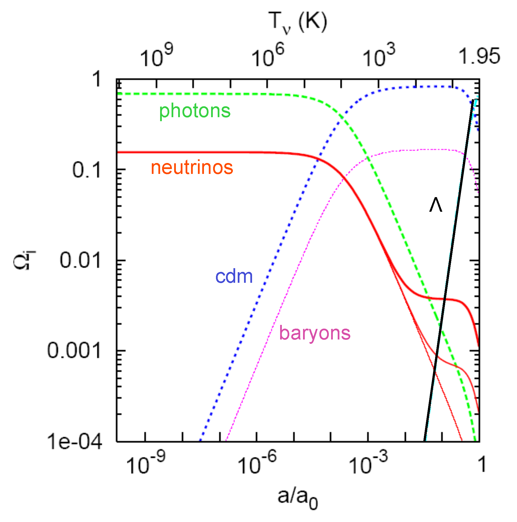
Throughout the Universe’s history, the neutrino with a small yet non-zero mass, as established previously from solar and atmospheric observations, will pass from being relativistic and part of the radiation budget to become non-relativistic and counted as part of the matter density in the Universe, as Figure 2 illustrates.
Thus, at early stages of the cosmological evolution, there exists a sea of neutrinos resulting from the interactions of the relic photons, the high density of which is a generic feature of the hot big bang theory. These neutrinos were produced at high temperatures by frequent weak interactions, and kept in equilibrium until these processes became ineffective when the rates of reactions became lower than the rate of expansion of the Universe and the latter cools. The temperature and momentum at the moment of decoupling can be found by supposing that their distribution is well described by a Fermi–Dirac method with a Gaussian average
where is the neutrino temperature and p is its momentum and a total energy density that is dominated by radiation. The number density is thus given by:
where is the Riemann zeta function of 3, integrating over the momentum in the last equality taken into account that for neutrinos. Then, by equating the thermally averaged value of the weak interaction rate to the Hubble parameter value, where is the cross-section of the electron–neutrino processes, with is the Fermi constant, is the neutrino number density, with the expansion rate given by the Hubble parameter from Friedman dominated by the radiation component (with being the Planck mass), and one finds roughly that dec ∼ 1 MeV is consistent with being relativistic. However, shortly after neutrino decoupling, the temperature drops below the electron mass, favoring e e annihilations into photons, which are heated by a factor that enters the ratio between the temperatures of relic photons and neutrinos. The contribution of neutrinos to radiation is then:
where is the photon density and the parameter accounts for any relativistic species which might be present at early times. With only three families of active neutrinos present in the standard model, the extra contribution with respect to the three families of active neutrinos () is an exact result of the complete treatment of neutrino decoupling, which takes into account non-instantaneous decoupling, finite-temperature QED-radiative corrections, and flavor oscillations [55].
This quantity encapsulates the radiation and neutrino densities that appear in the right-hand side of the Friedmann equation. In the ultrarelativistic () and non-relativistic () limits, the energy densities take simple analytic forms:
consistent with the fact that neutrinos behave as pressureless matter, , in the non-relativistic regime, and as radiation, , in the ultrarelativistic regime. These approximations will serve to better understand some of the neutrinos’ effects on observables that we will discuss later, as they allow us to have an estimation of the redshift , at which neutrinos of a given mass become non-relativistic. This is done, following the distribution above, by considering that the average momentum of neutrinos at a temperature , is taken at the moment of transition from the relativistic to the non-relativistic regime to be, as seen, , in light speed c = 1 unit. Then, using the fact that from Equation (7), eV, with being present-day cosmic microwave background (CMB) temperature to a good approximation, one has
We shall also need to determine the contribution of neutrinos to the matter–radation cosmological density equality. Given the present bounds on neutrino masses, we know that equality likely takes place around 3400 when neutrinos are relativistic. The radiation density is then provided by photons and by the relativistic neutrinos (and as such does not depend on the neutrino mass), plus any other light species present in the early Universe, so that the redshift of equivalence is given by
In the standard model, is fixed at ∼ 3.045. Therefore, the denominator of the previous equation is fixed. However, a change in modifies the total matter density at late times. This implies that, in a flat cosmological model, has to be modified accordingly to satisfy the flatness constraint, and thus the numerator is modified as well.
Given that the present-day neutrino temperature is fixed by measurements of the CMB temperature and by considerations of entropy conservation, we can, from the above formulas in Equation (6) write the total density parameter of massive neutrinos as:
3.2. Neutrino Late-Time Evolution
We also present here the redshift evolution of some of the quantity functions of neutrinos that will further help in the determination of their effects on the formation of structures. One that is relevant is the velocity dispersion. From the Fermi–Dirac distribution (5), we find a rough estimate:
For values of 1 eV for neutrinos close to present-day constraints, is comparable to the typical value of a galaxy. Thus, neutrinos, in contrast to cold dark matter that has by definition a vanishing , have too much thermal energy to be squeezed into small volumes to hierarchically form the structures we observe today [56]. However, this only means that neutrinos cannot account for dark matter but will still leave imprints on structure formation through their escape from matter potential at a free-streaming scale function of redshift. This is due to the fact that neutrinos possess large thermal velocities for a considerable part of cosmic history, so they can free stream out of overdense regions, effectively canceling perturbations on small scales. To obtain that, we should relate a linear perturbation in the Fourier space to the neutrino density at a certain scale and a time variable [57]. Then, the neutrino number density per Fourier mode relative to the mean density is obtained by integrating Equation (6) over momenta p,
with a, the scale factor and the potential solution to Poisson equation
Using the definition , we obtain for the neutrino density fluctuations
which could be recasted after a first-order solution
Here, is but the free-streaming wave vector, defined as
with as the neutrino’s characteristic thermal speed. Thus, large Fourier modes in the neutrino density fluctuations are suppressed by a factor proportional to relative to their CDM counterparts, which will have implications on the observables obtained from the clustering of large-scale structures, such as galaxies for example.
4. Impact on Observables
Early attempts, precursors of the more specific cosmological implications of neutrino physics, were first limited to the global impact on the Universe’s history and evolution. In that regard, Alpher et al. (1953) [58] and Pontecorvo et al. (1961) [59] debated the possibility that neutrinos’ densities would be comparable with baryonic matter and the implications of this assumption. However, it was Gershtein and Zeldovith (1966) [60] who made the first seminal constraint when they derived the upper limit on the density of neutrinos by demanding that the latter high value does not overclose the Universe, i.e., should be less than unity, which implies, according to Equation (11), that the sum of the neutrino masses < 93 eV.
After these first seminal works and since, as we see later, the neutrinos’ impact is closely related to their cosmological history and evolution, and we shall try to follow the same chronological order and describe here their influence on observables going from a high redshift to current ones.
At very-high redshift, close to the very early epoch, three minutes after the "beginning" of the Universe, neutrinos would have had an impact on the big bang nucleosynthesis (BBN) process when its density is part of the radiation density, dominating the energy budget at these times and thus, according to Equation (7), fixes the expansion rate, which in turn fixes the produced abundances of light elements, in particular that of He. The latter is then confronted with measurements to put constraints on the neutrinos’ relativistic effective number and models encapsulated in the value of , as denoted in Section 3.
Heading to lower redshifts, we have previously seen that Equation (9) gives approximately the redshift of transition to the non-relativistic regime, which happens to be close to the epoch of recombination. However, we see from the influence of neutrinos on perturbations above the free-streaming scale (cf. Equation (17)) that being non-relativistic will thus have a distinct signature on CMB temperature angular correlations at the recombination epoch that are not observed by CMB experiments [61], so that we are able, by inserting the redshift of recombination in Equation (9) around 1090, to put an upper limit of < 1 eV on their sum of eigenstate masses.
4.1. Neutrino Effects on the CMB Power Spectrum
Neutrinos will have different effects on the CMB spectrum. We remind that the latter anisotropies are encoded in the power spectrum2 coefficients Cℓs, i.e., the coefficients of the expansion in the Legendre polynomials of the two-point angular correlation function on the angular scales . In the case of the temperature angular fluctuations in CMB, it is expressed as:
More theoretically, and to gain some further insights, we describe how temperature fluctuations measured from the CMB are related to radiation-matter inhomogeneities interactions, by the following approximate formula from references [62,63], assuming recombination happened fast near the surface of the last scattering, a condition allowing to separate source evolution calculations from geometrical complexity:
where the first term of the right-hand side is the temperature anisotropy in the point of the last scattering surface, the second term comes from the gravitational shift of the photons traveling along in gravitational potential fluctuations known as the early Sachs–Wolf (SW) effect. It is followed by the correction to this temperature coming from the conventional Doppler caused by the velocity of the baryon–photon fluid. The last term is relative to the integrated Sachs–Wolfe (ISW) effect. It describes how the CMB angular power spectrum is affected on large scales when passing through varying potentials on its way towards the observer.
The shape of the observed power spectra is the result of the processes taking place in the primordial plasma around the time of recombination. Therefore, we observe a series of peaks and troughs in the temperature power spectrum, corresponding to oscillation modes that were caught at an extreme of compression or rarefaction (the peaks), or exactly in phase with the background (the troughs). The typical scale of the oscillations is set by the sound horizon at the recombination , i.e., the distance traveled by an acoustic wave ( being the sound speed) from some very early time until , the redshift of recombination and the presence of baryons, which shifts the zero of the oscillations, introducing an asymmetry between even and odd peaks. Finally, the peak structure is further modulated by an exponential suppression, due to the Silk damping of photon perturbations. The height of the first peak also depends on the redshift of equivalence Equation (10) (which sets the enhancement in power due to the early SW effect). Thus, the acoustic peaks hold most the information by their amplitudes and position functions of the angular separations in the CMB anisotropies.
Different effects related to the neutrinos’ density value, effective number, or their transition from relativistic to massive particles, are then induced.
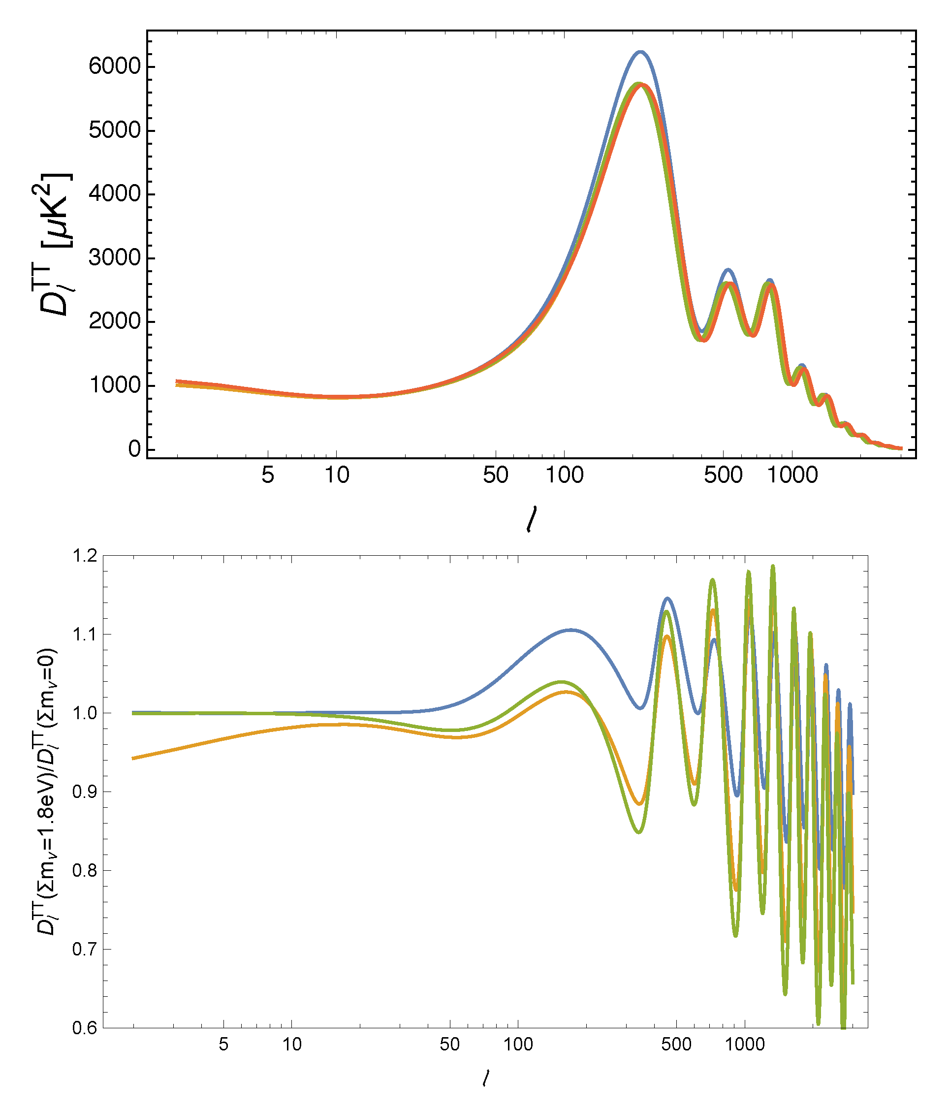
From being part of the radiation budget at the recombination epoch, the neutrino will change the expansion and impact the angular diameter distance (in the flat Universe for simplicity) to the last scattering surface , controlling the overall position of the CMB spectrum peaks in multipole space. This is degenerate with the matter density effect, including that on the slope of the low-ℓ tail of the CMB spectrum, due to the late-integrated Sachs–Wolfe (ISW) effect, but also with the redshift radiation-matter equality time that impacts the early SW effect. Figure 3 illustrates some of these effects, where the model in blue has a smaller with respect to the reference; the models in yellow and green have a larger (s for scattering); in addition, the yellow model also has a smaller (redshift of transition to dark energy domination over matter).
We also note another consequence of a change in the neutrino density, coming from different wavelengths entering at different epochs with changes in their time of travel following that of the expansion rate function of neutrino density. This impacts the early SW effect, which would stretch the position of the peaks. More neutrinos also imply stronger gravitational interactions between photons and free-streaming species before decoupling, which is important for scales that have just crossed the Hubble scale during the radiation domination epoch, resulting in a small shift and damping of the acoustic peak (“baryon drag” effect). This will also affect the “Silk” damping of the CMB anisotropies, as a higher changes the scale of this damping relative to the scale of the sound horizon at decoupling, which appears as a shift in the damping envelope of high peaks relative to the position of the first peak.
More secondary effects would also be generated from the neutrinos, later becoming non-relativistic and massive when, according to Equation (17), they escape the halo’s potential and slow the growth of the formation of large-scale structures, thus affecting the late ISW effect at low ell but also modifying the lensing from the large-scale structures on the multipoles. We end by a final subtle effect, when neutrinos, becoming non-relativistic, reduce the time variation of the gravitational potential inside the Hubble radius, affecting the photon temperature through the early SW effect, leading to a depletion in the temperature spectrum.
4.2. Effects of Neutrino on Large-Scale Structure Formation
Before we present the effect of massive neutrinos on large-scale structure formation, we first mention their impact on the baryonic acoustic oscillation (BAO) signal or the relic signature of the first peak in CMB, showing in-galaxy clustering through an enhancement in the amplitude of their angular correlation function of the angular distance . As we shall see later, this distance probe at relatively much lower redshift than that of the epoch of recombination of the CMB (but measured at different times), could, through the contribution of the neutrino’s density to the angular distance , break the matter density or Hubble constant’s total neutrino masses’ degeneracy and thus allow the first peak of the CMB spectrum to put stronger constraints on the neutrino’s density. Other geometric measurements such as those coming from the luminosity distance of SNIa can play the same role, as well as direct measurements of that rely on local distance indicators that are little or not-at-all dependent on the underlying cosmological model.
We move next to the matter domination epoch, where large-scale structure (LSS) formation mainly happens. There, the neutrino’s effect would be to mainly suppress growth rate, while its effect on the matter–radation redshift value will impact the LSS power spectrum formation, and from changes in the time density waves enter the gravitational horizon scale.
As an example to the influence of the first effect, we discuss the impact of neutrino density variation on the LSS power spectrum. Most LSS-related observables have the power spectrum as one of their ingredients, among them for example, the clustering of matter at large scales, a powerful probe of cosmology that can be described in terms of the two-point correlation function, or, equivalently, of , the power spectrum of matter density fluctuations:
where is the Fourier transform of the matter density perturbation at redshift z. Note that, contrarily to the CMB, we are bound to observe at a single redshift (that of recombination), that the matter power spectrum can, in principle, be measured at different times in the cosmic history, thus allowing for a tomographic and cross-correlations analysis resulting in strong constraints in parameters, such as the total neutrino masses, as we see next.
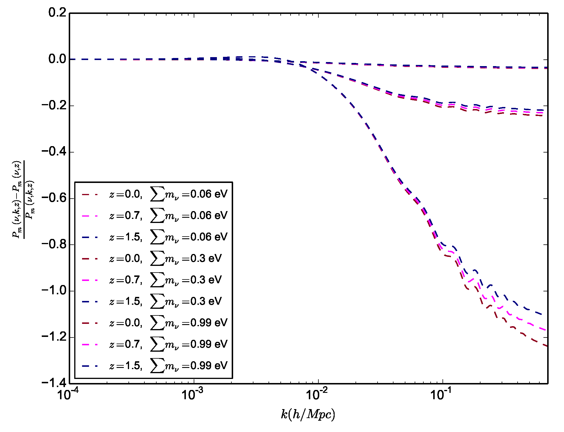
So, a first consequence of massive neutrino free-streaming is that, below the free-streaming scale, there is a smaller amount of matter that can cluster. This results in an overall suppression of the power spectrum at small scales, with respect to the neutrinoless case. Secondly, similar to what we observed in CMB interactions, subhorizon perturbations in the non-relativistic (i.e., cold dark matter and baryons) components grow more slowly. In fact, while in a perfectly matter-dominated Universe the gravitational potential is constant and the matter perturbation grows linearly with the scale factor with , in a mixed-matter–radation Universe, the gravitational potential decays slowly inside the horizon. Below the free-streaming scale, neutrinos effectively behave as radiation; then, in the limit in which the neutrino fraction is small, one has for
while is for .
These two effects can be approximated by the ratio [65]. This is illustrated in Figure 4, where we observe higher depletion with the increment of the mass of neutrinos while showing also a bigger effect at low masses with respect to high redshifts. Note that hierarchical neutrinos will each modify the power spectrum at slightly different free-streaming scales due to their individual masses, which allow to constrain hierarchy in principle, though it will be very difficult to disentangle these subtle signatures from the noise and the variance in the data.
As a consequence, we will be able to use an observable at slightly higher redshift than BAO as a stronger probe to the neutrinos’ mass: the forest of small clustering of matter detected by the Lyman- signal that are very sensitive to the free streaming of neutrinos.
Another consequence from a larger neutrino mass and less clustering on small scales is to decrease lensing by affecting the path of the photons coming from distant sources, since those photons will be deflected by the gravitational potentials along the line of sight. For CMB, this modifies the anisotropy pattern by mixing photons that come from different directions. In the temperature and polarization power spectra, the result is that the peaks and troughs at high ℓs are sharper. Additionally, lensing, being a non-linear effect, creates some amount of non-Gaussianity in the anisotropy pattern that can be detected and measured by looking at higher-order correlations in the CMB, offering another independent probe through the measured four-point correlation function referred to by the CMB lensing power spectrum. Neutrino mass is here constrained by its impact on the smoothing of the latter power spectrum at high ℓs. The power spectrum of the lensing potential is also detected from the measurements of the lensing-induced ellipticity of background galaxies with an effect more constraining than CMB when all the LSS lensing systematics are further reduced because it can be probed at different epochs, allowing a tomographic fix of the neutrino masses.
We shall show later the latest constraints from CMB, BAO, SN, and direct measurements of and LSS, each alone or in combination, but we note here that the CMB and BAO seems to prefer a null or very low value for the neutrinos’ mass in difference with higher ones coming from structure formation or lensing.
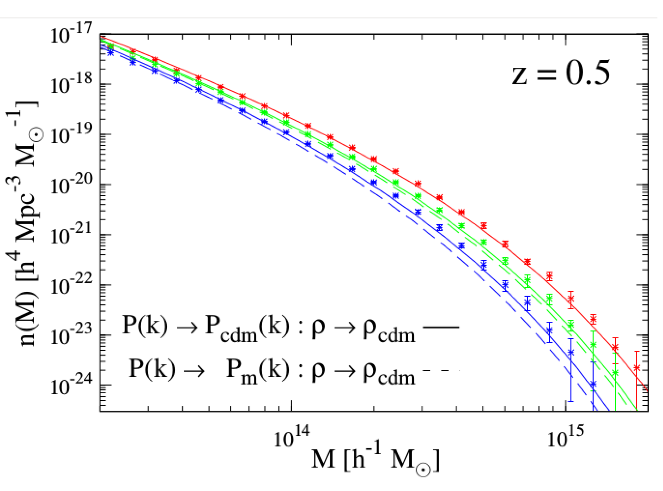
On the non-linear effect, it has been shown by Costanzi et al. [66] and Castorina et al. [67] that the determination of the non-linear matter power spectrum or the matter fluctuation parameter with massive neutrinos agrees with simulations if we only take the cdm+baryon power spectrum in a halo model approach to construct the non-linear power spectrum, or if we want to compute . This is shown in Figure 5, where this prescription falls better within the error bars from simulated haloes than the one with the full power spectrum.
Finally, of the remaining recent-used probes to constrain neutrino properties, we mention cosmic voids on which cosmological neutrinos have great influence, since these are the regions with the highest neutrino-to-dark-matter density ratios.
5. Constraints from Current Cosmo Datasets
Here, we present the latest constraints from single or combined probes on the active neutrino masses, their effective number, as well as bounds on the mass of a possible additional sterile massive neutrino. Concerning bounds on the latter, if it were to thermalize with the same temperature as active neutrinos, then it would be effectively similar to adding another flavor and would be close to ∼4. However, is usually left free to vary along with the sterile neutrino mass to allow more general thermalization mechanisms.
5.1. Neutrino Bounds from CMB and Combination with Other Geometrical Probes
We start by bounds from the CMB spectrum data before adding other probes. This is due to the fact that the CMB temperature-temperature (TT) spectrum, as seen in Section 4, shows numerous sensitivities in its features coming from the role of neutrinos in the different physical processes involved. This would limit the space of variation of neutrino proprieties, such as mass or number, since they need to accommodate for different phenomena at once. Though some degeneracies could arise, as the same effects could happen from varying other cosmological parameters, combining and crisscrossing with the EE spectrum or CMB lensing, as well as other external additional probes, will first allow to disentangle the role of each parameter; secondly, by constraining independently some of the other parameters, it will make the CMB-induced features able of strongly constraining neutrino properties.
Note that some of these probes are in tension with the CMB TT spectrum, such as the CMB lensing potential to some extent [23], or more strongly with some other local observables, such as LSS growth probes [68] on the matter fluctuation parameter , or with local distance probes, such as Cepheid’s and supernova’s constraints. This could result in best value shifting or further tightening on the neutrinos mass or effective relativistic number. However, this should be considered with the high degree of carefulness required when combining discordant data probes. Thus, this issue will be discussed in the next Section 6, while here, we present the current bounds in addition to those coming from works that used these conflicted measurements regardless of the previous warning.
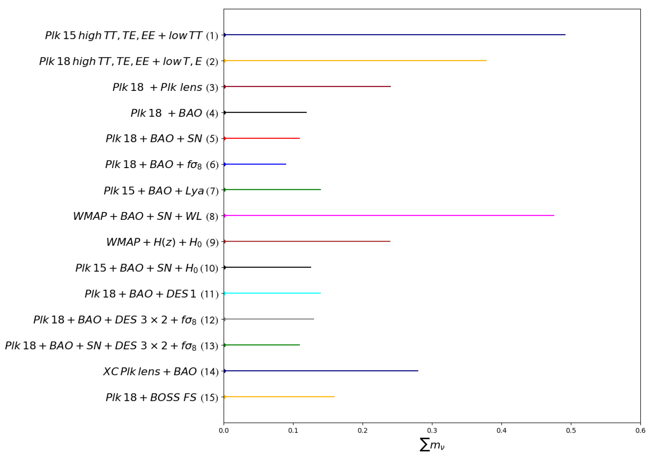
More specifically, the latest release from the Planck mission on CMB correlations in 2018 [23] yielded < 0.379 at (95% from Planck TT,TE,EE+low T,E), i.e., the full that we can extract from the data collected with an improvement from < 0.492 at (95% from Planck TT,TE,EE) in 2015 [69] before adding the low-ℓ polarization spectrum that helps to constrain , the degenerate parameter with the CMB power amplitude, to reach < 0.241 at (95% from Planck TT,TE,EE+low T,E+lensing)) in the final release in 2018 [23]. The big improvement also comes from the simultaneous addition of the lensing spectrum bringing further constraints from the neutrino mass effect on the large-scale lensing structure along our observation line of sight. The effective number of relativistic neutrinos was constrained to 2.92 ± 0.36 at 95% while combining with BBN, which has strong constraints on (as we noted in Section 4) and yielded = 3.04 with tighter bounds of at 95%.
Making use of BAO [23,70] substantially improves this limit to 0.12 eV (95%, Planck TT,TE,EE+lowE+lensing+BAO) and yields the number of relativistic neutrinos = 2.90 ± 0.17 at 95% if left free while < 3.29 ± 0.826 if we additionally consider a sterile neutrino with the latter mass < 0.65 eV. Further adding the latest supernovae (SNe) luminosity distance probe from Pantheon [24,71] data marginally tightens the bound to < 0.11 eV (95%, Planck TT,TE,EE+low T,E+lensing+BAO+Pantheon). We then need an observable where the effect of neutrinos in slowing the growth of structure is prominent to further tighten our constraints. Using the latest determinations of the growth rate parameter from RSD, which are a further independent measurement, along with CMB and a newer BAO data sample DR12 [72], Di Valentino (2021) [12] were able to set the most constraining bound to date to < 0.09 eV at 95% confidence contours (C.L.), with almost equal bounds when the number of relativistic particles is set free with < 0.095 eV and = 3.05 ± 0.33 at 95% C.L.
These two works are in agreement with bounds from the completed and extended study by the BOSS collaboration [25], which combined the results from the SDSS survey [73], BAO and redshift-space distortions (RSD), CMB from Planck, Pantheon Type Ia supernovae (SNe Ia), and the Dark Energy Survey (DES) [74] weak lensing to obtain < 0.11 eV at 95%, with the DES preferring a higher value of , pushing the limit by one point up, even with constraints from SN data.
These bounds are not far from those inferred from the Lyman-alpha probe, which are very sensitive to neutrinos, as seen in Section 4. In their latest release, Yeche et al. (2017) [75] obtained values for the cosmological parameters, including neutrinos in excellent agreement with the values derived independently from Planck 2015 CMB data. Combining BOSS and XQ-100 Ly power spectra, they constrained the sum of neutrino masses to < 0.8 eV (95% C.L.); when they are combined with CMB data 2015 only, this bound is tightened to < 0.14 eV (95% C.L.), which is very close to those inferred from the more recent Planck 2018 combined with BAO.
The above bounds were all on the sum of neutrino masses regardless of the hierarchy considered. In reference [70], combined Planck cosmic microwave background (CMB) temperature anisotropies and baryon acoustic oscillations (BAO) data, as well as the constraints on the optical depth to reionization (), show that the two aforementioned combinations disfavor the IH at ∼64% C.L. and ∼71% C.L. respectively, while reference [76], combining acoustic oscillation in the extended baryon oscillation spectroscopic survey (eBOSS) DR14 quasar sample with the temperature and polarization anisotropies power spectra of the cosmic microwave background from the Planck 2015 data, as well as low-redshift observations from the supernovae of type Ia and the local measurement of the Hubble constant, obtained the 95% confidence level upper limit to be < 0.129 eV for the degenerate mass hierarchy, < 0.159 eV for the normal mass hierarchy, and < 0.189 eV for the inverted mass hierarchy.
Local measurements of the Hubble parameter, as well as data from the cluster count or weak lensing, though in discrepancy with CMB data (see Section 6), have been also used to put constraints on neutrinos mass. Here, we show only the upper bounds obtained, which are still consistent with a non-detection, and leave results reporting partial mass detection from similar discrepant probes to Section 6.
As so, Wang et al. (2012) [77] used Hubble measurements in combination with the latest CMB, WL, BAO, and SNIa back then to provide a total neutrino masses upper limit of < 0.476 eV (95% C.L.), while Moresco et al. (2012a) [78] used a compilation of observational Hubble parameter data along with a local measurement of in combination with CMB WMAP data to put upper limits on the total neutrino masses < 0.24 eV at 68% C.L. and on their effective number = 3.45 ± 0.33 at 68%, which are both competitive with Planck releases with BAO bounds at the epoch. They also obtained = 3.45 ± 0.33. More recently, Di Valentino et al. (2016) [79] used Planck 2015 with BAO, SNIa, and locally, prior and in combination with tSZ cluster count data to find 95% C.L. constraint of < 0.126 eV. Di Valentino et al. also found < 0.2 eV and < 0.356 when the two were left free, as well as < 0.506 eV and 3.478 when a sterile neutrino was additionally considered, similar to Wang et al. (2018) [80], who obtained < 0.196 eV and = 2.984 ± 0.826, or Guo et al. (2019) [81], with 3.25 ± 0.15 when left free, alone, or with massive neutrinos, and an upper limit < 0.357 when varied with a sterile neutrino with a mass < 0.359 eV, while more recently, Feng et al. (2021) [82] used CMB + BAO + SN + H0 data to reach 3.54 ± 0.18 and < 0.12 eV.
All the above are competitive, even though some are combined with CMB data from earlier releases of Planck because of the use of discrepant probes in combination.
5.2. Constraining a Neutrino from Its Effect on the Growth of LSS
This is not always the case when combining with cluster counts or weak lensing correlations probes, where the discrepancy is not as high as with the local Hubble constant measurements, since this could lead to a loosening of the constraints on with respect to the combination of only CMB with other probes, because constraints from lensing or cluster probes push the neutrino masses’ values far from their minimum one. As so, constraints obtained from DES after the first-year data galaxy clustering and weak lensing release [83], which initially preferred lower values for value than the Planck CDM best-fit drove the neutrino masses to < 0.14 eV (95%, from Planck TT,TE,EE+low T,E+lensing+BAO+DES), not far from the recent three-year Dark Energy Survey results [84], where cosmological constraints from galaxy clustering and weak lensing and their cross-correlations (DES 3 × 2 pt data) combined with available baryon acoustic oscillations signals, a redshift-space distortions probe, type Ia supernovae data, and Planck CMB lensing, yielding < 0.13 eV (95% C.L.). Though additional, more accurate local RSD data, from the latest release of the SDSS survey [25], along with the previous combination of Planck, Pantheon SNe, SDSS BAO, and DES 3 × 2 pt data, reduced this value to < 0.11 (95%), it still remained higher than <0.09, the value previously mentioned as being obtained without DES but with similar other probes in combination.
Constraints could also come from a more in-depth treatment of the cross-correlations between the aforementioned probes. As so, cross-correlations between Planck 2015 CMB lensing only, without the TT and EE spectrum, and spectroscopic samples from BOSS, have been considered in Doux et al. (2017) [85], resulting in an upper limit of < 0.28 eV (68% C.L.), close to < 0.21 eV (95% C.L.) for Planck 2015 TT + lowP + BAO.
Finally, we mention another novel probe, based on the properties of massive neutrinos, to slow down the growth of the structures investigated by Ivanov et al. (2019) [86], who made use of a new full-shape (FS) likelihood for the redshift-space galaxy power spectrum of the BOSS data based on an improved perturbation theory. It yielded, when combined with Planck data, an upper limit on the sum of neutrino masses < 0.16 eV, and constraints on the effective number of extra relativistic degrees of freedom, = 2.88 ± 0.17.
Below, we compile most of the upper bounds mentioned above in one Figure 6 to better picture the status and compare the capabilities of the different probes or their combinations in constraining properties on the neutrino masses.
6. Neutrinos and Cosmological Tensions
The CDM model has succeeded in accommodating for most of the cosmological observations (see Section 1 for more details). However, two of its main parameters, the Hubble constant and the matter fluctuation one , are showing discrepancy when inferred using different probes, which seem to be divided mostly between deep ones, such as the CMB spectrum, versus local ones, such as distance from Cepheids for the Hubble parameter [87], or cluster counts and weak lensing shear correlations for (see Section 1 or reference [88] and references therein for more details).
6.1. Neutrinos as Possible Solution to the Cosmological Discrepancies
Due to the fact that they could weakly, within the current constraints, change the expansion and more strongly suppress the growth, neutrinos were advocated as a possible solution to ease these tensions. Thus, many have tried to fix one or both discrepancies by allowing the neutrino mass to vary.
In that regard, starting with the Hubble parameter, we have previously mentioned the work by Di Valentino et al. (2016) [79], who noticed that adding a prior on significantly improved the bounds on . We further detail this here, mentioning that the addition of the = 73 prior was found to have a much larger impact than a = 70 one, suggesting by converse that an ease of the Hubble tension is possible by more massive neutrinos. Others investigated whether solving the Hubble tension would require a sizable amount of extra radiation during recombination. As so, Guo et al. (2019) [81], previously mentioned in Section 5, found that the CDM + model is favored by the current observations, and that it can reduce the Hubble tension to be at the 1.87 level. It also pointed to many previous studies (see references therein) in which considering extra relativistic degrees of freedom in the CDM model favors a high value of when > 3.046. However, these findings will be undermined by the fact that the amount of is unavoidably constrained by big bang nucleosynthesis (BBN) in the early Universe (see Section 5). Schöneberg et al. (2019) [89] also reached this conclusion when they combined BAO, deuterium, and helium data, and found that the Hubble parameter is still in tension with the SHOES [27] measurements, even after allowing to vary from its fiducial value.
There were also attempts to test the impact of the neutrino mass on the growth of structure, hence possibly solving the discrepancy. Dvorkin et al. (2014) [28] tried by varying neutrino properties to reconcile measurements between the early and late Universe. They found evidence for different from the standard 3.046 and a one detection of a non-vanishing mass for a sterile neutrino from combining clusters and CMB probes.
The same was suggested by Wyman et al. (2014) [29], where the minimal neutrino model likelihood, i.e., a vanishing and a null sterile neutrino mass, was found far from the maximum likelihood when the clusters and CMB probes were combined. Leistedt et al. (2014) [90] also followed a similar investigation but showed that the tension remained when they considered extensions to the minimal neutrino model after combining the datasets. This later result could be due to the fact that, in all schemes, they added a BAO probe, which strongly constrains the neutrino mass. However, Beutler et al. (2014) [91] used the Planck temperature power spectrum with BAO from BOSS CMAS, combined with RSD and weak lensing measurements, to find a 3.4 preference for non-zero neutrino masses with = 0.36 ± 0.1, while when they simultaneously freed and the effective number of relativistic species, they found that = 3.61 ± 0.35 and = 0.46 ± 0.18 eV. The reason could be that they overlooked the possible effects of neutrino masses on their BAO scale determination, since they directly used the ones obtained from an excess of correlations constructed from the position of galaxies measured with a fiducial close to null neutrino mass.
At the same time, and staying with attempts involving the growth of LSS probes, Costanzi et al. (2014) [92] obtained a value, for active massive neutrinos this time, of ∼0.28 ± 0.2 eV (95%) when they combined the CMB spectrum and galaxy clusters counts.
More recently, Emami et al. (2017) [93] found that the clustering amplitude of richness detected by RedMaPPer algorithm clusters from the Sloan Digital Sky Survey (SDSS) increases with cluster mass with an excess to the cold dark matter predictions from simulations that could be accounted for by a total neutrino mass of = 0.119 ± 0.034 eV at 68% confidence level.
Finally, we remind of results in the previous section, showing that the full DES first-year data, when combined with Planck 2015 release and BAO, favored higher neutrino masses than Plk15 and BAO alone, relaxing its bound to < 0.14 eV instead of 0.12 eV. The same was confirmed with the three-year data release (see previous Section 5 for details).
Here, we show additional similar combinations that rather pointed to a neutrino mass detection, i.e., a maximum likelihood at masses far from the null value. Thus, early CMB data from Planck + galaxy cluster abundance from the South Pole telescope (SPT) polarization measurements survey [94] +BAO yielded a detection at 2 of (68% C.L.). However, de Haan et al. (2016) [95], while simultaneously freeing and the effective number of relativistic species, yielded = 3.28 ± 0.20 and = 0.18 ± 0.09 eV. Moreover and more recently, of all the probes at the pixel map level, as well as spectroscopic galaxy samples from the BOSS DR12 and KiDS weak lensing survey [96], the so-called 13 × 2-point analysis, consisting of a tomographic-combined analysis using a total of 10 auto- and 36 cross-spherical harmonic power spectra with CMB TT and EE and CMB lensing measurements from the Planck 2018 data, which was released by Sgier et al. (2021) [97], almost yielded a detection at ∼2.3 with = 0.51 + 0.21 −0.24 eV (68% C.L.).
6.2. Neutrinos’ Inability to Alleviate the Cosmological Tensions
However, all the above conclusions suggesting that massive neutrinos could solve the discrepancy should be considered with high carefulness, since they all originated as the result of combining two or more discrepant probes. This raises the question of the legitimacy of combining probes to extract tighter bounds in such situations, as so many works have revisited this subject with different approaches, either testing the ability of neutrinos to fix the discrepancy or comparing the behavior of the space of parameters’ constraints between each probe alone or by extending the number of parameters when combining, making the mass observable-calibration parameter, known to degenerate with or , or the luminosity calibration parameter , degenerate with .
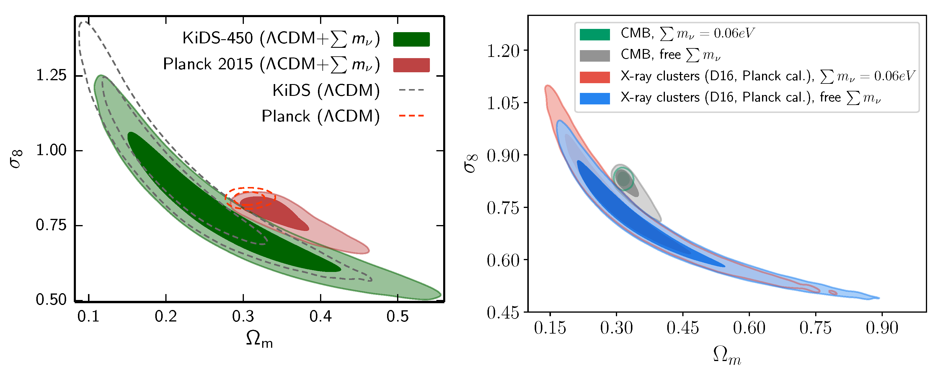
As so, Joudaki et al. (2017) [30] compared − likelihood contours obtained using the CMB power spectrum from Planck 2015 against weak lensing shear correlations from KiDS mission without combining them, and showed that neutrinos have no ability to fix the discrepancy, since the two likelihood contours change when allowing massive neutrinos in the same direction of the degeneracy instead of being orthogonal to it (cf. Figure 7), while Sakr et al. (2018) [31] and Ilic et al. (2019) [68] tested the impact of massive neutrinos on the − likelihood contours obtained from combining the CMB spectrum from Planck 2015 and the cluster counts detected in the X-ray and tSZ-detected cluster samples, leaving the mass observable-calibration of the clusters free to vary, showing that the latter likelihood is insensitive to the mass of neutrinos. Salvati et al. (2018) [98] also combined the tSZ power spectrum to the CMB spectrum, but they added BAO as an additional constraining tool for neutrinos and allowed freedom to the tSZ cluster count’s calibration factor around value. They reached the same conclusion that the mass bias to reconcile CMB and tSZ probes remains low at (1 − b) ∼ 0.67, even if we allow massive neutrinos.
This is in agreement with previous precursor studies, e.g., Roncarelli et al. (2015) [99], who tried to include neutrinos in simulations and detect clusters based on halo finders. Though they found that the number of detected clusters is reduced with massive neutrinos and concluded on the ability of neutrinos to fix the discrepancy. However, the effect of neutrinos on cluster count was almost degenerate with the combination of and , i.e., the same cluster counts with massive neutrinos obtained with a value of for a certain can be obtained with null-mass neutrinos for a higher value of and a lower value of ; thus, neutrino masses can take any value regardless of the − combination. Additionally, Bohringer et al. (2016) [100] found no significant massive neutrino effect on the − likelihood from REFLEX II X-ray cluster counts. They also found in reference [101] that the change in the cluster mass function determined from the observed cluster X-ray luminosity distribution from adding neutrinos was smaller than the uncertainties related to the determination of the cluster mass function.
Finally, we note another "healthy" treatment that is rather suggesting a detection, or higher neutrino masses, this time, but conducted on CMB data itself when comparing the consistency of the constraints from effects of lensing on CMB against those from the lensing power spectrum constructed from the same measurements before combining them. This could be performed by introducing a consistency parameter , scaling the theoretical expectation for each observable with , indicating a full agreement which is usually set to the unity value because the two observables did not disagree to more than 2 . However, Di Valentino and Melchiorri (2021) [102] found that allowing the to vary suggested neutrino masses from Plk 18 + Plk lensing to be = 0.41 0.2 eV at 68%, consistent with "Planck-independent" combinations, such as Plk lensing with the data of the CMB Atacama cosmology telescope [103]. ACT-DR4+WMAP+Lensing suggesting also = 0.6 ± 0.25 eV at 68%, or CMB polarization and temperature correlation measurements from the South Pole telescope [104], with SPT-3G+WMAP+Lensing yielding at 68% level.
7. A Closure from Next-Generation Surveys?
Different upcoming experiments that can potentially be used to improve our constraints on the sum of neutrino masses are reviewed below, along with forecasts, with differences in the degrees of maturity in terms of the theoretical understanding of the processes involved when analyzing the data and differences in the optimization of the relevant survey’s mission. Though some experiments are not to be mainly conceived for neutrinos mass detection, the latter is nevertheless obtained when the other cosmological parameters, with similar effects on the observables (see Section 4), are constrained.
We shall follow the same path as when we explored the landscape of current probes and their constraining power on neutrinos, using instead the next upcoming generation of the cosmological common or more innovative probes, starting with the future improvement of CMB spectrum-detection experiments, alone, or combined with the different planned methods of measuring LSS clustering through electromagnetic observations or lensing, before finishing with even further proposed novelties. The bounds will be shown at the 68% confidence level unless stated otherwise.
For the CMB future experiments, they could be of a ground-based or space-borne nature, where the greatest contaminant for the former is the atmospheric noise reducing the microwave-accessible frequencies. On the other hand, ground-based experiments benefit from the ability to use a larger collecting area with a very high number of detectors with respect to the space-borne ones. A key target for them is a better determination of the current relatively less constrained , the uncertainty of which limits the ability to compare the amplitude of primordial fluctuations from the CMB to the amplitude of matter perturbations from late-universe probes (cf. Section 4). As an example, the proposed CMB polarization measurements experiments PIXIE [105], CORE [20], and CLASS [106] would achieve an almost cosmic-variance-limited (CVL) detection of the reionization optical depth . More generally, Allison et al. (2015) [107] and Yu et al. (2018) [108] both studied the improvements on the total neutrino masses as a function of the increase of the accuracy on the determination of from the combination of probes and the stage of the experiments. Furthermore, the ability of measuring with high precision the small-scale polarization will allow us to reconstruct the lensing potential with higher accuracy, enabling us to break more degeneracies between the cosmological parameters and the neutrino mass (see [109] for an extensive review on the subject).
Constraints from the galaxy distributions are also planned along with the CMB, despite the effect of neutrinos on the power spectrum becoming smaller with redshift, since the neutrinos would have less time to delay the growth of CDM+baryons perturbations on small scales; however, going to higher redshifts will allow a larger survey volume, which with higher sensitivity and collecting time, will be able to measure small scales sensitive to neutrinos’ linear- and non-linear-dependent effects. Additionally, tomographic measurements of the late-time universe will be sensitive to the different redshift dependence of the signatures of massive neutrinos and this will increase the robustness of their mass estimates from cosmology. The near-planned LSS surveys could be broken down into two categories: distance constraints (BAO, AP [110], etc.) and constraints from the growth of structures (the shape and amplitude of the matter power spectrum, RSD [111], etc.). As mentioned, the two could be also probed by lensing effects, such as strong ones modifying the shape of the LSS, resulting in distance-constrained or weak ones, for which the measurements of the galaxy distribution lensing shear serves as the equivalent of a galaxy spectrum usually detected from collecting lights from emitting sources.
It remains to solve theoretical issues as to the ability of benefiting from all the small scales. The survey could probe where non-linear or baryonic effects will become prominent with respect to linear and cold dark matter-only physics. Caution about possible complications such as higher-order biasing and systematic errors in the analysis of high redshift galaxy clustering that may be non-negligible should also be taken, or else we will be forced to cut the level of our understanding, losing valuable information. An example illustrating that is the work of Vagnozzi et al. (2017) [70], who found that the constraining power of measurements of the full-shape galaxy power spectrum is less powerful than the BAO signature from the BOSS survey, despite the measurements covering a larger volume with smaller error bars compared to previous similar measurements due to the conservative analysis method commonly adopted, which is due to the lack of a good theoretical understanding of neutrino effects on smaller scales.
After overcoming these challenges, we can benefit from the extension of the combination of the actual Stage III to Stage IV upcoming probes. An example would be through the use of CMB correlations with the accurate cosmological distance and measurements of galaxy distributions and combinations among them before they are all convolved by lensing effects. These could also be used as a probe by themselves to obtain similar but stronger probes than the actual 3 × 2 or 13 × 2 cross-correlations we have seen in Section 5.
Besides, we can obtain further information about the neutrino mass from observations of the HI distribution in, around, or after the reionization epoch, when the 21 cm line of radiation is emitted long after the recombination and before the start of the LSS formation. This will give us information on the relativistic level, as well as exploring matter perturbations at the linear regime on most of the scales, which can be analytically calculated when they are not affected by non-linearities. Moreover, these futuristic 21 cm surveys will also map an extremely large volume of the Universe and constrain the growth of structures at the epoch of reionization, thus limiting the cosmic variance from the former and limiting the need to account for baryonic feedback for the latter.
At this time, we are expecting Stage-IV next-generation surveys to start delivering data from the beginning of next year with DESI spectroscopic [18] and eROSITA galaxy clusters surveys [112], with more to come in short intervals during the next decade. That is why there have been many attempts to forecast on neutrino constraints benefiting from different appropriate combinations of the planned surveys to push the limits of the forecast presented in the survey definition book of each individual mission. This combination is necessary as, for example, two classes of future CMB mission proposals, CORE or CMB-S4 [17], cannot achieve alone the necessary sensitivity to claim a detection of = 0.06 eV at the 3 level.
7.1. Review of Forecasts from Next-Generation Surveys on the Mass and Number of Neutrino Species
We review next some of the forecasts from different studies conducted in the last decade, and finish with a summary plot at the end.
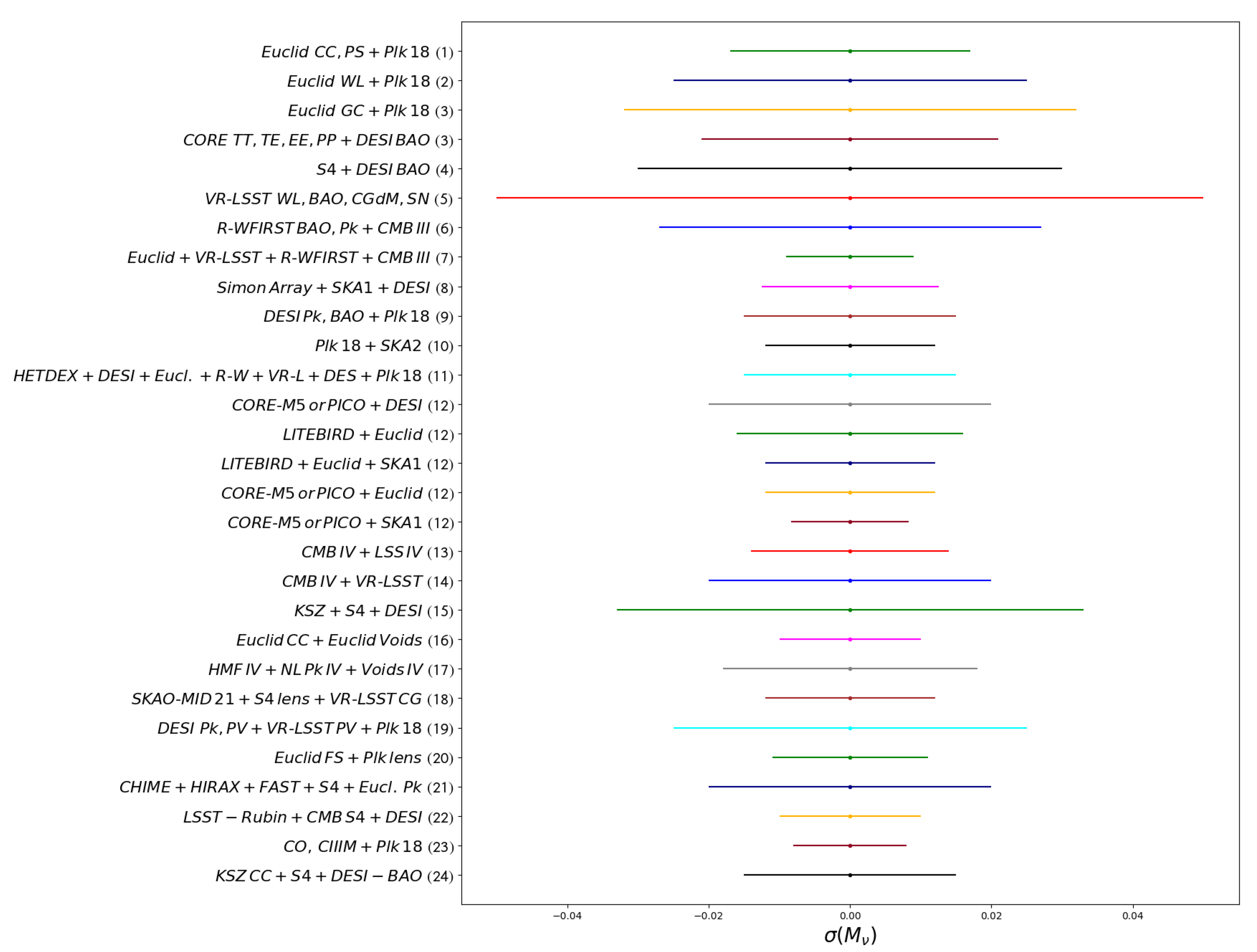
Audren et al. (2013) [113] made one of the first attempts in 2013 to forecast on neutrino masses from an Euclid survey trying also to account for uncertainties in the modeling of the effect of neutrinos on the non-linear galaxy power spectrum with the assumptions that they increase with the ratio of a given scale to the scale of non-linearity, which hence increases with wavenumber and decreases with redshift. They found that a future Euclid-like cosmic shear/galaxy survey would achieve a 1- error on close to 0.032 eV/0.025 eV, while assuming instead a 10 times smaller theoretical error decreases it to ) = 0.018 eV/0.014 eV. Within the same survey, supposing that the probes in tension on could be combined to obtain constraints on the neutrino mass, Cerbolini et al. (2013) [114] combined information from an Euclid-like cluster number count and cluster power spectrum along with data from the cosmic microwave background (CMB) measurements from Planck to obtain = 0.017 eV, while additionally allowing a free yielded a = 0.07 and = 0.022 eV. More recently, Chudaykin et al. (2019) [115] used only galaxy clustering from Euclid but with a complete perturbation theory model for the galaxy one-loop power spectrum and tree-level bispectrum, to obtain, in the most optimistic case when combining with Planck lensing data, comparable bounds with ) = 0.011 eV.
Moving to CMB-based planned surveys, combining CORE TT,TE,EE,PP, and DESI BAO yielded an error down to ) = 0.021 eV, with a ∼3 detection in the minimal mass scenario [20], in the same range as of the case of CMB S4 + DESI BAO [17], where Abazajian et al. (2016) found that ) bounds fall in the range of 0.023–0.036 eV, not far from the previously mentioned Allison et al. (2015) [107], who combined Stage-IV CMB experiments with DESI BAO to obtain a tighter range (0.015–0.029) after, however, supposing an improvement on the optical depth measurement.
Additionally, the DESI collaboration (2016) [18] forecasted on the total neutrino masses, including all possible probes by the survey, and found using BAO information from DESI galaxies, quasars, and the Ly- forest, along with the broadband galaxy power spectrum and Planck constraints, that ) = 0.02 eV, while = 0.062.
These are not far from the Euclid constraints mentioned above but also from LSST-Rubin survey [14]. The latter will provide multiple probes of the late-time evolution of the Universe with a single experiment, namely, weak lensing cosmic shear, BAO in the galaxy power spectrum, an evolution of the mass function of galaxy clusters, and a compilation of SNIa redshift distances with an expected sensitivity of in the range ) = 0.030–0.070 eV. Among the next-generation LSS surveys, we mention the WFIRST-Roman telescope [15], which will test the late expansion of the Universe with great accuracy by employing supernovae, weak lensing, BAO, redshift-space distortions (RSD), and clusters as probes. Thus, from the BAO and broadband measurements of the matter power spectrum, WFIRST-Roman in combination with a Stage-III CMB experiment could provide ) < 0.03 eV [15]. Finally, adding all in an appropriate combination of WFIRST-Roman, Euclid, LSST-Rubin, and CMB Stage III can achieve almost double or more precision than each survey alone with ) < 0.01 eV [15].
Constraints could also come from combining with future wide and deep radio surveys. Oyama et al. (2016) [116] showed that precise ground-based CMB polarization observations, such as Simons Array along with a 21 cm line observation, such as the square kilometer array (SKA) phase one and a baryon acoustic oscillation observation, such as DESI, can measure, through their effect on the growth of density fluctuation, a non-zero neutrino mass to ∼ 0.02 at 95% C.L. Additionally, the combinations can strongly improve errors of the bounds on the effective number of neutrino species to ∼0.06–0.09 at 95% C.L. Finally, by using SKA phase two instead of one, they reached ) < 0.15 eV.
Sprenger et al. (2019) [117] found with Planck+SKA2 that the total neutrino masses could be constrained to ) = 0.012 eV with the baseline model, assuming a realistic theoretical error, leading to a 5 -detection, while additionally allowing a free yields and 0.014 eV. Along the same line, Ballardini (2021) [118] forecasted using a multi-tracer analysis in order to reduce cosmic variance and combined a SKA-MID 21 cm intensity map with Stage-IV CMB lensing along with galaxy clustering from LSST-Rubin, finding that = 0.012 eV. Obuljen et al. (2018) [119] also focused on radio probes in the redshift range 2.5 < z < 5 through suitable extensions of existing and upcoming radio surveys, such as CHIME [120], HIRAX [121], and FAST [122], and reached, when combining with CMB S4 and galaxy clustering from Euclid, = 0.02 eV and a very competitive constraint on relativistic number of neutrinos, namely = 0.02.
Tighter constraints could be in principle forecasted to be obtained from combining a larger set of the available future experiments. One of the early attempts was by Font-Ribera et al. in 2014 [123], who combined DESI and generally redshift spectroscopically-detected galaxy surveys (BOSS, HETDEX, eBOSS, Euclid, and WFIRST-Roman), and also included CMB from (Planck) and weak gravitational lensing (DES and LSST-Rubin) constraints on redshift surveys to forecast on the sum of neutrino masses reaching a 0.011 eV, while additionally allowing that a free would yield = 0.041 and = 0.013 eV. This was not far from similar constraints from Boyle et al. (2018) [124], who used the same upcoming probes, forecasting around 0.025 eV, or the previously mentioned Yu et al. (2018) [108] who combined LSST-Rubin + CMB S4 + DESI but with a prior on to reach = 0.01 eV.
Finally, Brinckmann et al. (2019) [125] tested exhaustively 35 different combinations, including the above future cosmic microwave background-based ones and large-scale structures data to set bounds on cosmological parameters and the total neutrino masses under conservative assumptions when accounting for uncertainties in the modeling of systematics, removing for galaxy surveys the information coming from highly non-linear scales.
In particular, they highlighted the performances of the following combinations in terms of confidence metrics, which we present below but with additional corresponding limits on the neutrino masses and effective number. Subsequently, they showed that:
CORE-M5 and PICO are so sensitive that they would only need to be combined with the BAO scale data from DESI for a 3 detection on with , while additionally allowing that a free yields and 0.021 eV.
A 3 to 4 detection on could be achieved already by Planck or LiteBIRD when combined with Euclid with , while additionally allowing that a free yields and 0.021 eV.
LiteBIRD in combination with Euclid and SKA1 intensity mapping reaches the 5 threshold on with , while additionally allowing that a free yields and 0.017 eV.
CORE-M5 or PICO would also achieve a 5 detection on in combination with Euclid only, with , while additionally allowing that a free yields and 0.014 eV.
CORE-M5 or PICO would even achieve a 7 detection on when SKA1 intensity mapping data is added, and a 10 one if reio could be further constrained with bounds from the former on , while additionally allowing that a free yields and 0.0099 eV and tighter ones from the latter on , while additionally allowing that a free yields and 0.0078 eV.
This illustrates the benefit towards a precise neutrino mass detection from having a very accurate independent determination of the optical depth from surveys focused on reionization and the dark ages, such as LiteBIRD and CORE-M5, in comparison with the only 2 to 3 detection achieved by LSS experiments, such as Euclid and SKA, even when combined with CMB-S4.
This is also in line with the white paper from Dvorkin et al. (2019) [126], in which they stated that with the current sensitivity of = 0.007, next-generation surveys will result in an almost 3 detection of the minimal mass allowed by oscillation experiments, while a combination of next-generation CMB and LSS surveys has the potential to reach a nearly 4 detection corresponding to a ) = 0.014 eV. The later prediction was also emphasized by Mishra-sharma et al. (2019) [127], projecting that future CMB measurements combined with late-time measurements of galaxy clustering and cosmic shear from the large synoptic survey telescope would achieve a 3 measurement of the minimal 0.06 eV mass, and 4 with, however, a five-fold-improved measurement of the optical depth to reionization, obtainable through a large-scale CMB polarization measurement.
This is also similar to Archidiacono et al. (2020) [21], who used future CMB data with future weak lensing photometric observations (WL), future spectroscopic galaxy clustering surveys (GC), and neutral hydrogen 21 cm intensity mapping (IM) from CMB-S4+LiteBIRD+Euclid+SKA1- IM-B2 missions to test three scenarios: “realistic”, “optimistic”, and “extreme”, with the first using the same assumptions of reference [117]. The optimistic assumes that the systematic errors are under control, while the extreme assumes that there is no theoretical uncertainty on the modeling of non-linear clustering on small scales. They found, when assuming the degenerate approximation, i.e., the fiducial values of each of the three neutrinos is set to the minimum mass of each hierarchy, a 3 detection of the neutrino mass in the first two cases, while it was more than 5 for the last case. Again, a better determination of is crucial and seems to dominate the best bounds on neutrino masses and effective relativistic numbers since Ansari et al. (2019) [128] or, more recently, Sailer et al. (2021) [129], even when considering a highly optimistic scenario when combining, along with the next Stage-IV experiments mentioned above, probes that reach redshifts z or above with one order of magnitude higher galaxy-number density and higher sky coverage, such as SPHEREX [130], MSE [131], HIRAX [121], MegaMapper [132], and PUMA [133], which could not achieve equal or slightly better than 0.01 eV and without the inclusion of LiteBird experiments.
7.2. Further Forecasts on Bounds from New Probes on the Mass of Neutrino Number of Species
We finish by reporting on future constraints from less common or newly suggested probes. Already we have evoked the use of the bispectrum probe by Chudaykin et al. (2019) [115], who showed that constraints improve when they are combined with the more common power spectrum probe, or Cerbolini et al. (2013) [114], who combined information from Euclid-like cluster number counts and the cluster power spectrum along with data from the cosmic microwave background (CMB) measurements from Planck to obtain competitive constraints with respect to the above combinations of the different surveys’ primary probes. We continue with Visbal et al. (2009) [134], who proposed to use 21 cm emissions from residual neutral hydrogen after the epoch of reionization to trace the cosmological power spectrum of density fluctuations and reached 0.03 eV on the neutrino mass. Mueller et al. (2015) [135] introduced a forecast from the scale dependency of neutrinos on the power spectrum used to determine the mean pairwise momentum of clusters observed through the kinematic Sunyaev–Zel’dovich (kSZ)3 and obtained an upper limit on the of 0.11 eV at 68% when combined with Stage-IV CMB and DESI spectroscopic galaxy survey future missions, a limit that will improve to 0.033 eV if the averaged optical depth of clusters can be measured with few percent accuracy. Along the same lines, Madhavacheril et al. (2017) [136] used catalogs of galaxy clusters produced through the thermal Sunyaev–Zel’dovich (tSZ) effect from future high-resolution measurements of the cosmic microwave background (CMB) with self-calibrating mass observables, or those calibrated by measuring the lensing signal around these clusters, to obtain ) < 0.01 eV at 68% when combined with BAO from DESI and a prior on the reionization parameter. This is slightly better then Bolliet et al. (2019) [137], who forecasted on bounds of neutrino masses using tSZ galaxy clusters and a power spectrum with , along with CMB-S4+DESI-BAO, a 1% accuracy on the mass calibration and a masking on the heavy clusters to limit contamination with large-scale CMB to reach ) at 68%.
As a complementary to galaxy clusters, Sahlen et al. (2019) [138], for minimal normal-hierarchy neutrino masses, forecasted that Euclid’s clusters and voids, independent of other data, very ideally could reach uncertainties, such as ) ≲ 0.01 eV, even when considering further extensions to CDM, such as , the dark energy equation of the state parameter. Though we do not explore extra extensions to CDM in this review, the constraints on (w0) ≲ 0.003 are so strong from this combination that they do not expect to change significantly those on the neutrinos’ mass. This is in agreement with Bayer et al. (2021) [139], who quantified the information content of the non-linear matter power spectrum, the halo mass function, and the void size function, using the Quijote N-body simulations. He found that these three statistics exhibit very different degeneracies amongst the cosmological parameters, and thus the combination of all three probes enables the breaking of degeneracies, yielding remarkably tight constraints on the marginalized error of the sum of neutrino masses ) = 0.018 eV. The former values could be further improved using independent data from other surveys. As so, the forecast conducted by Weltman et al. (2018) [140] combining SKA2 voids and Euclid cluster counts showed that we could reach as low as ) = 0.002 eV.
Among other new observables, Whitford et al. (2021) [141] are proposing to use measurements of galaxy-peculiar velocities from future LSST-Rubin and DESI spectroscopic measurements along with a CMB Planck spectrum to obtain ) = 0.025, while additionally allowing a free , which yielded = 0.07 and = 0.035 eV. The novelty could come by benefiting from new proxies to the matter density fields. As so, inspired from the intensity mapping analysis of HI lines’ future observations from the SKA survey, Dizgah et al. (2021) [142] are proposing to use wide-field ground-based mm-wavelength surveys of line intensity mapping to measure the auto-power spectra of several CO rotational lines and the CII fine-structure ones in the redshift range of 0.25 < z < 12, and those obtained in optimistic cases with very strong ) < 0.01, while 68% error reached 0.022 after only combining with the CMB from Planck 2018 data sets.
Finally, many works [143,144,145,146] are forecasting improvements in the constraints on neutrino masses from the impacts of the gravitational wave (GW) standard future siren observations, such as the Einstein telescope (ET), the cosmic explorer (CE), or the Taiji future ground GW detectors. They mostly simulated 1000 GW events that would be observed after 10 years observation and found improvements of around 20% with respect to actual bounds.
Below, we compile most of the bounds mentioned above in one Figure 8 to better picture the status and capabilities of the different upcoming probes or their combinations in constraining properties on the neutrino mass.
8. Discussion and Conclusions
In this paper, we have presented the status of the constraints on the neutrino masses and the effective number of species obtained from the current, as well as forecasts from future cosmological probes. After reviewing the impact of the aforementioned neutrino’s properties on the process involved in the Universe’s background and large-scale structures formation dynamics, and evolution, we have also discussed the potential of neutrinos to alleviate the present tensions observed on the Hubble and matter density fluctuations parameters when determined from local probes against those from deep probes.
We noted that the total neutrino masses and number of species are strongly constrained by the combination of the CMB spectrum and are rich in neutrino-sensitive features, with less deeper distance measurements to break degeneracies with other cosmological parameters effects, while adding large-scale structure probes, the growth of which are substantially slowed by neutrino mass and might further lower the upper limit on the total neutrino masses to one from the lowest possible value of 0.06 eV, which was inferred from terrestrial or astrophysical experiments. We also highlighted that solving the tensions on the Hubble or the matter fluctuation parameter between the local and deep probes of distance or LSS probes would require almost a detection at 2 on the neutrino total mass in certain scenarios, providing that its variation is not further constrained by other independent probes. However, we also presented some studies that followed more appropriate approaches to combine discrepant datasets, as is the case with the aforementioned tensions, and showed that neutrinos are not fundamentally able of alleviating the tensions, regardless of the additional constraints that further probes might have brought.
We finally reviewed the different forecasts conducted in view of the advent of the next-generation Stage-IV surveys (or even beyond) in constraining neutrino properties and found that we could ultimately go down to below the 10 percent precision necessary to detect at more than 5 the total neutrino masses or its effective number of species, providing that we combine with probes that can constrain the averaged optical depth, the only parameter then remaining in degeneracy with neutrino properties, to a few percent of accuracy.
However, all these experiments, mostly sensitive to the sum of neutrino masses, might not be able to determine the right neutrino hierarchy if the fiducial mass is high enough, such as >0.1 or 0.15, as noted by Archidiacono et al. (2021) [21], because correlations between nuisance and cosmological parameters could mimic the tiny deviations induced by the hierarchies. We already saw that with MegaMapper [132], though it was more sensitive than the Stage-IV surveys. Additionally, among the forecasts presented above, Oyama et al. (2016) [116] tested in addition the ability of future surveys to disentangle between hierarchies, and showed that they can determine the neutrino mass hierarchy at 95% C.L. only if the total neutrino mass is similar to or smaller than 0.1 eV.
Thus, we have to wait until experiments such as the GAUSS-proposed future mission [147], which has a very deep flux limit and a very high multiplexing capability allowing to map unique tracers from redshift 0.5 to 5.0 with limited systematics, and which also has the power of probe combinations and their cross-correlation within a single experiment, which will surpass by more than an order of magnitude all currently foreseen Stage-IV projects hoping to reach the hierarchy detection goal. Beside non-cosmological-based experiments such as the Deep Underground Neutrino Experiment (DUNE) [148,149] and the Jiangmen Underground Neutrino Observatory [150], that detailed review is outside the scope of this review, the complementarity with which could reduce the space of variation of the neutrino mass, and we could also hope that other experiments, such as PTOLEMY [151], which is aiming to detect the hypothetical cosmic neutrino background (CNB) with properties similar to the CMB but with deeper redshifts and neutrino physics as the main actor, or the futuristic 21 cm surveys (e.g., the fast Fourier transform telescope [152]) mapping an extremely large volume of the Universe, at the epoch of reionization, when it was not affected by non-linearities or baryonic feedback, will enable us to achieve the aforementioned objectives.
Funding
This research received no external funding.
Acknowledgments
The author would like to acknowledge the administrative support from Miranda Song and thank the referees for their relevant comments and recommendations.
Conflicts of Interest
The author declares no conflict of interest.
| 1 | See [48] for a detailed study on perspectives for neutrino flavor conversions determinations in other astrophysical and cosmological environments. |
| 2 | the power spectrum being the 3D Fourier transform of the correlation function. |
| 3 | similar to the tSZ effect, the kSZ effect is the imprint of galaxy clusters on CMB from peculiar motion and is proportional to the integrated electron momentum along the line-of-sight. |
References
- Capozzi, F.; Lisi, E.; Marrone, A.; Montanino, D.; Palazzo, A. Neutrino masses and mixings: Status of known and unknown 3ν parameters. Nucl. Phys. B 2016, 908, 218–234. [Google Scholar] [CrossRef] [Green Version]
- Robertson, R.G.H.; Bowles, T.J.; Stephenson, G.J.; Wark, D.L.; Wilkerson, J.F.; Knapp, D.A. Limit on anti-electron-neutrino mass from observation of the beta decay of molecular tritium. Phys. Rev. Lett. 1991, 67, 957–960. [Google Scholar] [CrossRef] [PubMed]
- Kraus, C.; Bornschein, B.; Bornschein, L.; Bonn, J.; Flatt, B.; Kovalik, A.; Ostrick, B.; Otten, E.W.; Schall, J.P.; Thümmler, T.; et al. Final results from phase II of the Mainz neutrino mass search in tritium beta decay. Eur. Phys. J. C 2005, 40, 447–468. [Google Scholar] [CrossRef]
- Aseev, V.N.; Belesev, A.I.; Berlev, A.I.; Geraskin, E.V.; Golubev, A.A.; Likhovid, N.A.; Lobashev, V.M.; Nozik, A.A.; Pantuev, V.S.; Parfenov, V.I.; et al. An upper limit on electron antineutrino mass from Troitsk experiment. Phys. Rev. D 2011, 84, 112003. [Google Scholar] [CrossRef] [Green Version]
- Aker, M.; Beglarian, A.; Behrens, J.; Berlev, A.; Besserer, U.; Bieringer, B.; Block, F.; Bobien, S.; Boettcher, M.; Bornschein, B.; et al. Direct neutrino-mass measurement with sub-electronvolt sensitivity. Nat. Phys. 2022, 18, 160–166. [Google Scholar] [CrossRef]
- Alfonso, K. Search for Neutrinoless Double-Beta Decay of 130Te with CUORE-0. Phys. Rev. Lett. 2015, 115, 102502. [Google Scholar] [CrossRef] [Green Version]
- Colgate, S.A.; White, R.H. The Hydrodynamic Behavior of Supernovae Explosions. Astrophys. J. 1966, 143, 626. [Google Scholar] [CrossRef]
- Avrorin, A.D.; Avrorin, A.V.; Aynutdinov, V.M.; Bannash, R.; Belolaptikov, I.A.; Brudanin, V.B.; Budnev, N.M.; Doroshenko, A.A.; Domogatsky, G.V.; Dvornický, R.; et al. Baikal-GVD: Status and prospects. EPJ Web Conf. 2018, 191, 01006. [Google Scholar] [CrossRef]
- Abbasi, R.; Ackermann, M.; Adams, J.; Ahlers, M.; Ahrens, J.; Andeen, K.; Auffenberg, J.; Bai, X.; Baker, M.; Barwick, S.W.; et al. The IceCube Data Acquisition System: Signal Capture, Digitization, and Timestamping. Nucl. Instrum. Meth. A 2009, 601, 294–316. [Google Scholar] [CrossRef] [Green Version]
- Ageron, M.; Aguilar, J.A.; Al Samarai, I.; Albert, A.; Ameli, F.; André, M.; Anton, G.; Anvar, S.; Ardid, M.; Arnaud, K.; et al. ANTARES: The first undersea neutrino telescope. Nucl. Instrum. Meth. A 2011, 656, 11–38. [Google Scholar] [CrossRef]
- Adrian-Martinez, S.; Ageron, M.; Aharonian, F.; Aiello, S.; Albert, A.; Ameli, F.; Anassontzis, E.; Andre, M.; Androulakis, G.; Anghinolfi, M.; et al. Letter of intent for KM3NeT 2.0. J. Phys. G 2016, 43, 084001. [Google Scholar] [CrossRef]
- Di Valentino, E.; Gariazzo, S.; Mena, O. Most constraining cosmological neutrino mass bounds. Phys. Rev. D 2021, 104, 083504. [Google Scholar] [CrossRef]
- Laureijs, R.; Amiaux, J.; Arduini, S.; Augueres, J.L.; Brinchmann, J.; Cole, R.; Cropper, M.; Dabin, C.; Duvet, L.; Ealet, A.; et al. Euclid Definition Study Report. arXiv 2011, arXiv:1110.3193. [Google Scholar]
- LSST Science, Collaboration; Abell, P.A.; Allison, J.; Anderson, S.F.; Andrew, J.R.; Angel, J.R.P.; Armus, L.; Arnett, D.; Asztalos, S.J.; Axelrod, T.S.; et al. LSST Science Book, Version 2.0. arXiv 2009, arXiv:0912.0201. [Google Scholar]
- Spergel, D.; Gehrels, N.; Baltay, C.; Bennett, D.; Breckinridge, J.; Donahue, M.; Dressler, A.; Gaudi, B.S.; Greene, T.; Guyon, O. et al.Wide-Field InfrarRed Survey Telescope-Astrophysics Focused Telescope Assets WFIRST-AFTA 2015 Report. arXiv 2015, arXiv:1503.03757. [Google Scholar]
- Bacon, D.J.; et al.; [Square Kilometre Array Cosmology Science Working Group] Cosmology with Phase 1 of the Square Kilometre Array: Red Book 2018: Technical specifications and performance forecasts. Publ. Astron. Soc. Austral. 2020, 37, e007. [Google Scholar] [CrossRef] [Green Version]
- Abazajian, K.N.; Adshead, P.; Ahmed, Z.; Allen, S.W.; Alonso, D.; Arnold, K.S.; Baccigalupi, C.; Bartlett, J.G.; Battaglia, N.; Benson, B.A.; et al. CMB-S4 Science Book, First Edition. arXiv 2016, arXiv:1610.02743. [Google Scholar]
- Aghamousa, A.; et al.; [DESI Collaboration] The DESI Experiment Part I: Science,Targeting, and Survey Design. arXiv 2016, arXiv:1611.00036. [Google Scholar]
- Hazumi, M.; Ade, P.A.R.; Adler, A.; Allys, E.; Arnold, K.; Auguste, D.; Aumont, J.; Aurlien, R.; Austermann, J.; Baccigalupi, C.; et al. LiteBIRD: JAXA’s new strategic L-class mission for all-sky surveys of cosmic microwave background polarization. Proc. SPIE Int. Soc. Opt. Eng. 2020, 11443, 114432F. [Google Scholar] [CrossRef]
- Di Valentino, E.; Brinckmann, T.; Gerbino, M.; Poulin, V.; Bouchet, F.R.; Lesgourgues, J.; Melchiorri, A.; Chluba, J.; Clesse, S.; Delabrouille, J.; et al. Exploring cosmic origins with CORE: Cosmological parameters. JCAP 2018, 4, 017. [Google Scholar] [CrossRef] [Green Version]
- Archidiacono, M.; Hannestad, S.; Lesgourgues, J. What will it take to measure individual neutrino mass states using cosmology? JCAP 2020, 9, 21. [Google Scholar] [CrossRef]
- Kowalski, M.; Rubin, D.; Aldering, G.; Agostinho, R.J.; Amadon, A.; Amanullah, R.; Balland, C.; Barbary, K.; Blanc, G.; Challis, P.J.; et al. Improved Cosmological Constraints from New, Old and Combined Supernova Datasets. Astrophys. J. 2008, 686, 749–778. [Google Scholar] [CrossRef] [Green Version]
- Aghanim, N.; et al.; [Planck Collaboration] Planck 2018 results. VI. Cosmological parameters. Astron. Astrophys. 2021, 641, A6, Erratum in Astron. Astrophys. 2021, 652, C4. [Google Scholar] [CrossRef] [Green Version]
- Scolnic, D.; Brout, D.; Carr, A.; Riess, A.G.; Davis, T.M.; Dwomoh, A.; Jones, D.O.; Ali, N.; Charvu, P.; Chen, R.; et al. The Pantheon+ Type Ia Supernova Sample: The Full Dataset and Light-Curve Release. arXiv 2021, arXiv:2112.03863. [Google Scholar]
- Alam, S.; et al.; [eBOSS Collaboration] Completed SDSS-IV extended Baryon Oscillation Spectroscopic Survey: Cosmological implications from two decades of spectroscopic surveys at the Apache Point Observatory. Phys. Rev. D 2021, 103, 083533. [Google Scholar] [CrossRef]
- Ade, P.A.R.; et al.; [Planck Collaboration] Planck 2015 results. XXIV. Cosmology from Sunyaev-Zeldovich cluster counts. Astron. Astrophys. 2016, 594, A24. [Google Scholar] [CrossRef] [Green Version]
- Riess, A.G.; Yuan, W.; Macri, L.M.; Scolnic, D.; Brout, D.; Casertano, S.; Jones, D.O.; Murakami, Y.; Breuval, L.; Brink, T.G.; et al. A Comprehensive Measurement of the Local Value of the Hubble Constant with 1 km/s/Mpc Uncertainty from the Hubble Space Telescope and the SH0ES Team. arXiv 2021, arXiv:2112.04510. [Google Scholar]
- Dvorkin, C.; Wyman, M.; Rudd, D.H.; Hu, W. Neutrinos help reconcile Planck measurements with both the early and local Universe. Phys. Rev. D 2014, 90, 083503. [Google Scholar] [CrossRef] [Green Version]
- Wyman, M.; Rudd, D.H.; Vanderveld, R.A.; Hu, W. Neutrinos Help Reconcile Planck Measurements with the Local Universe. Phys. Rev. Lett. 2014, 112, 051302. [Google Scholar] [CrossRef] [Green Version]
- Joudaki, S.; Mead, A.; Blake, C.; Choi, A.; de Jong, J.; Erben, T.; Conti, I.F.; Herbonnet, R.; Heymans, C.; Hildebrandt, H.; et al. KiDS-450: Testing extensions to the standard cosmological model. Mon. Not. Roy. Astron. Soc. 2017, 471, 1259–1279. [Google Scholar] [CrossRef] [Green Version]
- Sakr, Z.; Ilić, S.; Blanchard, A.; Bittar, J.; Farah, W. Cluster counts: Calibration issue or new physics? Astron. Astrophys. 2018, 620, A78. [Google Scholar] [CrossRef] [Green Version]
- Archidiacono, M.; Gariazzo, S. Two sides of the same coin: Sterile neutrinos and dark radiation. Status and perspectives. arXiv 2022, arXiv:2201.10319. [Google Scholar]
- Pauli, W. Letter to L. Meitner and her colleagues. Phys. Today 1930, 9, 23. [Google Scholar]
- Fermi, E. Versuch einer Theorie der β-Strahlen. I. Zeitschrift für Physik 1934, 88, 161–177. [Google Scholar] [CrossRef]
- Glashow, S.L. The renormalizability of vector meson interactions. Nucl. Phys. 1959, 10, 107–117. [Google Scholar] [CrossRef]
- Salam, A.; Ward, J.C. Weak and electromagnetic interactions. Nuovo Cim. 1959, 11, 568–577. [Google Scholar] [CrossRef]
- Weinberg, S. A Model of Leptons. Phys. Rev. Lett. 1967, 19, 1264–1266. [Google Scholar] [CrossRef]
- Reines, F.; Cowan, C.L. The neutrino. Nature 1956, 178, 446–449. [Google Scholar] [CrossRef]
- Goldhaber, M.; Grodzins, L.; Sunyar, A.W. Helicity of Neutrinos. Phys. Rev. 1958, 109, 1015–1017. [Google Scholar] [CrossRef] [Green Version]
- Majorana, E. Teoria simmetrica dell’elettrone e del positrone. Il Nuovo Cimento (1924–1942) 1937, 14, 171–184. [Google Scholar] [CrossRef]
- Pontecorvo, B. Mesonium and anti-mesonium. Sov. Phys. JETP 1957, 6, 429. [Google Scholar]
- Maltoni, M.; Schwetz, T.; Tortola, M.A.; Valle, J.W.F. Status of global fits to neutrino oscillations. New J. Phys. 2004, 6, 122. [Google Scholar] [CrossRef]
- Kajita, T. Nobel Lecture: Discovery of atmospheric neutrino oscillations. Rev. Mod. Phys. 2016, 88, 030501. [Google Scholar] [CrossRef] [Green Version]
- McDonald, A.B. Nobel Lecture: The Sudbury Neutrino Observatory: Observation of flavor change for solar neutrinos. Rev. Mod. Phys. 2016, 88, 030502. [Google Scholar] [CrossRef]
- de Salas, P.F.; Forero, D.V.; Ternes, C.A.; Tortola, M.; Valle, J.W.F. Status of neutrino oscillations 2018: 3σ hint for normal mass ordering and improved CP sensitivity. Phys. Lett. B 2018, 782, 633–640. [Google Scholar] [CrossRef]
- Esteban, I.; Gonzalez-Garcia, M.C.; Maltoni, M.; Schwetz, T.; Zhou, A. The fate of hints: Updated global analysis of three-flavor neutrino oscillations. JHEP 2020, 9, 178. [Google Scholar] [CrossRef]
- Formaggio, J.A.; de Gouvêa, A.L.C.; Robertson, R.G.H. Direct Measurements of Neutrino Mass. Phys. Rept. 2021, 914, 1–54. [Google Scholar] [CrossRef]
- Capozzi, F.; Saviano, N. Neutrino Flavor Conversions in High-Density Astrophysical and Cosmological Environments. Universe 2022, 8, 94. [Google Scholar] [CrossRef]
- de Gouvea, A.; Jenkins, J.; Kayser, B. Neutrino mass hierarchy, vacuum oscillations, and vanishing |U(e3)|. Phys. Rev. D 2005, 71, 113009. [Google Scholar] [CrossRef] [Green Version]
- Cappuzzello, F.; Agodi, C.; Cavallaro, M.; Carbone, D.; Tudisco, S.; Presti, D.L.; Oliveira, J.R.B.; Finocchiaro, P.; Colonna, M.; Rifuggiato, D.; et al. The NUMEN project: NUclear Matrix Elements for Neutrinoless double beta decay. Eur. Phys. J. A 2018, 54, 72. [Google Scholar] [CrossRef] [Green Version]
- Albanese, V.; et al.; [SNO+ Collaboration] The SNO+ experiment. JINST 2021, 16, P08059. [Google Scholar] [CrossRef]
- Barabash, A.S. Double Beta Decay: Historical Review of 75 Years of Research. Phys. Atom. Nucl. 2011, 74, 603–613. [Google Scholar] [CrossRef] [Green Version]
- Ejiri, H. Experimental Approaches to Neutrino Nuclear Responses for ββ Decays and Astro-Neutrinos. Front. Phys. 2021, 9, 82. [Google Scholar] [CrossRef]
- Lesgourgues, J.; Pastor, S. Neutrino cosmology and Planck. New J. Phys. 2014, 16, 065002. [Google Scholar] [CrossRef]
- de Salas, P.F.; Pastor, S. Relic neutrino decoupling with flavour oscillations revisited. JCAP 2016, 7, 51. [Google Scholar] [CrossRef]
- Tremaine, S.; Gunn, J.E. Dynamical Role of Light Neutral Leptons in Cosmology. Phys. Rev. Lett. 1979, 42, 407–410. [Google Scholar] [CrossRef]
- Ringwald, A.; Wong, Y.Y.Y. Gravitational clustering of relic neutrinos and implications for their detection. JCAP 2004, 12, 005. [Google Scholar] [CrossRef]
- Alpher, R.A.; Follin, J.W.; Herman, R.C. Physical Conditions in the Initial Stages of the Expanding Universe. Phys. Rev. 1953, 92, 1347–1361. [Google Scholar] [CrossRef]
- Pontecorvo, B.; Smorodinsky, Y. The neutrino and the density of matter in the universe. Z. Eksp. Teor. Fiz. 1961, 41, 239–243. [Google Scholar]
- Gershtein, S.S.; Zeldovich, Y.B. Rest Mass of Muonic Neutrino and Cosmology. JETP Lett. 1966, 4, 120–122. [Google Scholar]
- Gawiser, E.; Silk, J. The Cosmic microwave background radiation. Phys. Rept. 2000, 333, 245–267. [Google Scholar] [CrossRef] [Green Version]
- Sachs, R.K.; Wolfe, A.M. Perturbations of a cosmological model and angular variations of the microwave background. Astrophys. J. 1967, 147, 73–90. [Google Scholar] [CrossRef]
- Hu, W.; White, M.J. CMB anisotropies in the weak coupling limit. Astron. Astrophys. 1996, 315, 33. [Google Scholar]
- Gerbino, M.; Lattanzi, M. Status of neutrino properties and future prospects—Cosmological and astrophysical constraints. Front. Phys. 2018, 5, 70. [Google Scholar] [CrossRef]
- Hu, W.; Eisenstein, D.J.; Tegmark, M. Weighing neutrinos with galaxy surveys. Phys. Rev. Lett. 1998, 80, 5255–5258. [Google Scholar] [CrossRef] [Green Version]
- Costanzi, M.; Villaescusa-Navarro, F.; Viel, M.; Xia, J.Q.; Borgani, S.; Castorina, E.; Sefusatti, E. Cosmology with massive neutrinos III: The halo mass function andan application to galaxy clusters. JCAP 2013, 12, 012. [Google Scholar] [CrossRef]
- Castorina, E.; Sefusatti, E.; Sheth, R.K.; Villaescusa-Navarro, F.; Viel, M. Cosmology with massive neutrinos II: On the universality of the halo mass function and bias. JCAP 2014, 2, 049. [Google Scholar] [CrossRef]
- Ilić, S.; Sakr, Z.; Blanchard, A. Cluster counts. II. Tensions, massive neutrinos, and modified gravity. Astron. Astrophys. 2019, 631, A96. [Google Scholar] [CrossRef]
- Ade, P.A.R.; et al.; [Planck Collaboration] Planck 2015 results. XIII. Cosmological parameters. Astron. Astrophys. 2016, 594, A13. [Google Scholar] [CrossRef] [Green Version]
- Vagnozzi, S.; Giusarma, E.; Mena, O.; Freese, K.; Gerbino, M.; Ho, S.; Lattanzi, M. Unveiling ν secrets with cosmological data: Neutrino masses and mass hierarchy. Phys. Rev. D 2017, 96, 123503. [Google Scholar] [CrossRef] [Green Version]
- Scolnic, D.M.; Jones, D.O.; Rest, A.; Pan, Y.C.; Chornock, R.; Foley, R.J.; Huber, M.E.; Kessler, R.; Narayan, G.; Riess, A.G.; et al. The Complete Light-curve Sample of Spectroscopically Confirmed SNe Ia from Pan-STARRS1 and Cosmological Constraints from the Combined Pantheon Sample. Astrophys. J. 2018, 859, 101. [Google Scholar] [CrossRef]
- Dawson, K.S.; Kneib, J.-P.; Percival, W.J.; Alam, S.; Albareti, F.D.; Anderson, S.F.; Armengaud, E.; Aubourg, E.; Bailey, S.; Bautista, J.E.; et al. The SDSS-IV extended Baryon Oscillation Spectroscopic Survey: Overview and Early Data. Astron. J. 2016, 151, 44. [Google Scholar] [CrossRef]
- Loveday, J.; Pier, J. The Sloan Digital Sky Survey. 1998. Available online: http://xxx.lanl.gov/abs/astro-ph/9809179 (accessed on 19 March 2022).
- Abbott, T.; et al.; [Dark Energy Survey Collaboration] The Dark Energy Survey. 2005. Available online: http://xxx.lanl.gov/abs/astro-ph/0510346 (accessed on 19 March 2022).
- Yèche, C.; Palanque-Delabrouille, N.; Baur, J.; du Mas des Bourboux, H. Constraints on neutrino masses from Lyman-alpha forest power spectrum with BOSS and XQ-100. JCAP 2017, 6, 047. [Google Scholar] [CrossRef] [Green Version]
- Wang, S.; Wang, Y.F.; Xia, D.M. Constraints on the sum of neutrino masses using cosmological data including the latest extended Baryon Oscillation Spectroscopic Survey DR14 quasar sample. Chin. Phys. C 2018, 42, 065103. [Google Scholar] [CrossRef] [Green Version]
- Wang, X.; Meng, X.L.; Zhang, T.J.; Shan, H.; Gong, Y.; Tao, C.; Chen, X.; Huang, Y.F. Observational constraints on cosmic neutrinos and dark energy revisited. JCAP 2012, 11, 018. [Google Scholar] [CrossRef] [Green Version]
- Moresco, M.; Verde, L.; Pozzetti, L.; Jimenez, R.; Cimatti, A. New constraints on cosmological parameters and neutrino properties using the expansion rate of the Universe to z~1.75. JCAP 2012, 7, 053. [Google Scholar] [CrossRef] [Green Version]
- Di Valentino, E.; Giusarma, E.; Mena, O.; Melchiorri, A.; Silk, J. Cosmological limits on neutrino unknowns versus low redshift priors. Phys. Rev. D 2016, 93, 083527. [Google Scholar] [CrossRef] [Green Version]
- Wan, H.Y.; Cao, S.L.; Teng, H.Y.; Liu, Y.; Zhang, J.C.; Zhang, T.J. Direct constraint on cosmic neutrino mass using observational Hubble parameter data. Res. Astron. Astrophys. 2018, 18, 124. [Google Scholar] [CrossRef] [Green Version]
- Guo, R.Y.; Zhang, J.F.; Zhang, X. Can the H0 tension be resolved in extensions to ΛCDM cosmology? JCAP 2019, 02, 054. [Google Scholar] [CrossRef] [Green Version]
- Feng, L.; Guo, R.Y.; Zhang, J.F.; Zhang, X. Cosmological search for sterile neutrinos after Planck 2018. Phys. Lett. B 2022, 827, 136940. [Google Scholar] [CrossRef]
- Abbott, T.M.C.; et al.; [DES Collaboration] Dark Energy Survey year 1 results: Cosmological constraints from galaxy clustering and weak lensing. Phys. Rev. D 2018, 98, 043526. [Google Scholar] [CrossRef] [Green Version]
- Abbott, T.M.C.; et al.; [DES Collaboration] Dark Energy Survey Year 3 results: Cosmological constraints from galaxy clustering and weak lensing. Phys. Rev. D 2022, 105, 023520. [Google Scholar] [CrossRef]
- Doux, C.; Penna-Lima, M.; Vitenti, S.D.P.; Tréguer, J.; Aubourg, E.; Ganga, K. Cosmological constraints from a joint analysis of cosmic microwave background and spectroscopic tracers of the large-scale structure. Mon. Not. Roy. Astron. Soc. 2018, 480, 5386–5411. [Google Scholar] [CrossRef] [Green Version]
- Ivanov, M.M.; Simonović, M.; Zaldarriaga, M. Cosmological Parameters and Neutrino Masses from the Final Planck and Full-Shape BOSS Data. Phys. Rev. D 2020, 101, 083504. [Google Scholar] [CrossRef] [Green Version]
- Di Valentino, E.; Mena, O.; Pan, S.; Visinelli, L.; Yang, W.; Melchiorri, A.; Mota, D.F.; Riess, A.G.; Silk, J. In the realm of the Hubble tension—A review of solutions. Class. Quant. Grav. 2021, 38, 153001. [Google Scholar] [CrossRef]
- Perivolaropoulos, L.; Skara, F. Challenges for ΛCDM: An update. arXiv 2021, arXiv:2105.05208. [Google Scholar]
- Schöneberg, N.; Lesgourgues, J.; Hooper, D.C. The BAO+BBN take on the Hubble tension. JCAP 2019, 10, 029. [Google Scholar] [CrossRef] [Green Version]
- Leistedt, B.; Peiris, H.V.; Verde, L. No new cosmological concordance with massive sterile neutrinos. Phys. Rev. Lett. 2014, 113, 041301. [Google Scholar] [CrossRef] [Green Version]
- Beutler, F.; Saito, S.; Brownstein, J.R.; Chuang, C.-H.; Cuesta, A.J.; Percival, W.J.; Ross, A.J.; Ross, N.P.; Schneider, D.P.; Samushia, L.; et al. The clustering of galaxies in the SDSS-III Baryon Oscillation Spectroscopic Survey: Signs of neutrino mass in current cosmological data sets. Mon. Not. R. Astron. Soc. 2014, 444, 3501–3516. [Google Scholar] [CrossRef] [Green Version]
- Costanzi, M.; Sartoris, B.; Viel, M.; Borgani, S. Neutrino constraints: What large-scale structure and CMB data are telling us? JCAP 2014, 10, 081. [Google Scholar] [CrossRef] [Green Version]
- Emami, R.; Broadhurst, T.; Jimeno, P.; Smoot, G.; Angulo, R.; Lim, J.; Chu, M.C.; Yeung, S.; Zeng, Z.; Lazkoz, R. Evidence of Neutrino Enhanced Clustering in a Complete Sample of Sloan Survey Clusters, Implying ∑mν=0.119±0.034 eV. arXiv 2017, arXiv:1711.05210. [Google Scholar]
- Schaffer, K.K.; Crawford, T.M.; Aird, K.A.; Benson, B.A.; Bleem, L.E.; Carlstrom, J.E.; Chang, C.L.; Cho, H.M.; Crites, A.T.; De Haan, T.; et al. The First Public Release of South Pole Telescope Data: Maps of a 95-square-degree Field from 2008 Observations. Astrophys. J. 2011, 743, 90. [Google Scholar] [CrossRef] [Green Version]
- de Haan, T.; Benson, B.A.; Bleem, L.E.; Allen, S.W.; Applegate, D.E.; Ashby, M.L.N.; Bautz, M.; Bayliss, M.; Bocquet, S.; Brodwin, M.; et al. Cosmological Constraints from Galaxy Clusters in the 2500 square-degree SPT-SZ Survey. Astrophys. J. 2016, 832, 95. [Google Scholar] [CrossRef]
- Giblin, B.; Heymans, C.; Asgari, M.; Hildebrandt, H.; Hoekstra, H.; Joachimi, B.; Kannawadi, A.; Kuijken, K.; Lin, C.-A.; Miller, L.; et al. KiDS-1000 catalogue: Weak gravitational lensing shear measurements. Astron. Astrophys. 2021, 645, A105. [Google Scholar] [CrossRef]
- Sgier, R.; Lorenz, C.; Refregier, A.; Fluri, J.; Zürcher, D.; Tarsitano, F. Combined 13×2-point analysis of the Cosmic Microwave Background and Large-Scale Structure: Implications for the S8-tension and neutrino mass constraints. arXiv 2021, arXiv:2110.03815. [Google Scholar]
- Salvati, L.; Douspis, M.; Aghanim, N. Constraints from thermal Sunyaev-Zel’dovich cluster counts and power spectrum combined with CMB. Astron. Astrophys. 2018, 614, A13. [Google Scholar] [CrossRef] [Green Version]
- Roncarelli, M.; Carbone, C.; Moscardini, L. The effect of massive neutrinos on the Sunyaev–Zel’dovich and X-ray observables of galaxy clusters. Mon. Not. R. Astron. Soc. 2015, 447, 1761–1773. [Google Scholar] [CrossRef] [Green Version]
- Böhringer, H.; Chon, G. Constraints on neutrino masses from the study of the nearby large-scale structure and galaxy cluster counts. Mod. Phys. Lett. A 2016, 31, 1640008. [Google Scholar] [CrossRef] [Green Version]
- Böhringer, H.; Chon, G.; Retzlaff, J.; Trümper, J.; Meisenheimer, K.; Schartel, N. The extended Northern ROSAT Galaxy Cluster Survey (NORAS II) I. Survey Construction and First Results. Astron. J. 2017, 153, 220. [Google Scholar] [CrossRef]
- Di Valentino, E.; Melchiorri, A. Neutrino Mass Bounds in the era of Tension Cosmology. arXiv 2021, arXiv:astro-ph.CO/2112.02993. [Google Scholar]
- Aiola, S.; Calabrese, E.; Maurin, L.; Naess, S.; Schmitt, B.L.; Abitbol, M.H.; Addison, G.E.; Ade, P.A.R.; Alonso, D.; Amiri, M.; et al. The Atacama Cosmology Telescope: DR4 Maps and Cosmological Parameters. JCAP 2020, 12, 047. [Google Scholar] [CrossRef]
- Dutcher, D.; Balkenhol, L.; Ade, P.A.R.; Ahmed, Z.; Anderes, E.; Anderson, A.J.; Archipley, M.; Avva, J.S.; Aylor, K.; Barry, P.S.; et al. Measurements of the E-mode polarization and temperature-E-mode correlation of the CMB from SPT-3G 2018 data. Phys. Rev. D 2021, 104, 022003. [Google Scholar] [CrossRef]
- Kogut, A.J.; Chuss, D.T.; Dotson, J.L.; Fixsen, D.J.; Halpern, M.; Hinshaw, G.F.; Meyer, S.M.; Moseley, S.H.; Seiffert, M.D.; Spergel, D.N.; et al. The Primordial Inflation Explorer (PIXIE) Mission. Proc. SPIE Int. Soc. Opt. Eng. 2010, 7731, 77311S. [Google Scholar] [CrossRef]
- Watts, D.J.; Wang, B.; Ali, A.; Appel, J.W.; Bennett, C.L.; Chuss, D.T.; Dahal, S.; Eimer, J.R.; Essinger-Hileman, T.; Harrington, K.; et al. A Projected Estimate of the Reionization Optical Depth Using the CLASS Experiment’s Sample Variance Limited E-mode Measurement. Astrophys. J. 2018, 863, 121. [Google Scholar] [CrossRef] [Green Version]
- Allison, R.; Caucal, P.; Calabrese, E.; Dunkley, J.; Louis, T. Towards a cosmological neutrino mass detection. Phys. Rev. D 2015, 92, 123535. [Google Scholar] [CrossRef] [Green Version]
- Yu, B.; Knight, R.Z.; Sherwin, B.D.; Ferraro, S.; Knox, L.; Schmittfull, M. Towards Neutrino Mass from Cosmology without Optical Depth Information. arXiv 2018, arXiv:1809.02120. [Google Scholar]
- Errard, J.; Feeney, S.M.; Peiris, H.V.; Jaffe, A.H. Robust forecasts on fundamental physics from the foreground-obscured, gravitationally-lensed CMB polarization. JCAP 2016, 3, 052. [Google Scholar] [CrossRef] [Green Version]
- Alcock, C.; Paczynski, B. An evolution free test for non-zero cosmological constant. Nature 1979, 281, 358–359. [Google Scholar] [CrossRef]
- Percival, W.J.; White, M. Testing cosmological structure formation using redshift-space distortions. MNRAS 2009, 393, 297–308. [Google Scholar] [CrossRef] [Green Version]
- Borm, K.; Reiprich, T.H.; Mohammed, I.; Lovisari, L. Constraining galaxy cluster temperatures and redshifts with eROSITA survey data. Astron. Astrophys. 2014, 567, A65. [Google Scholar] [CrossRef] [Green Version]
- Audren, B.; Lesgourgues, J.; Bird, S.; Haehnelt, M.G.; Viel, M. Neutrino masses and cosmological parameters from a Euclid-like survey: Markov Chain Monte Carlo forecasts including theoretical errors. JCAP 2013, 1, 026. [Google Scholar] [CrossRef] [Green Version]
- Cerbolini, M.C.A.; Sartoris, B.; Xia, J.Q.; Biviano, A.; Borgani, S.; Viel, M. Constraining neutrino properties with a Euclid-like galaxy cluster survey. JCAP 2013, 6, 020. [Google Scholar] [CrossRef] [Green Version]
- Chudaykin, A.; Ivanov, M.M. Measuring neutrino masses with large-scale structure: Euclid forecast with controlled theoretical error. JCAP 2019, 11, 034. [Google Scholar] [CrossRef] [Green Version]
- Oyama, Y.; Kohri, K.; Hazumi, M. Constraints on the neutrino parameters by future cosmological 21 cm line and precise CMB polarization observations. JCAP 2016, 2, 008. [Google Scholar] [CrossRef]
- Sprenger, T.; Archidiacono, M.; Brinckmann, T.; Clesse, S.; Lesgourgues, J. Cosmology in the era of Euclid and the Square Kilometre Array. JCAP 2019, 2, 047. [Google Scholar] [CrossRef] [Green Version]
- Ballardini, M.; Maartens, R. Constraining the neutrino mass using a multi-tracer combination of two galaxy surveys and CMB lensing. arXiv 2021, arXiv:2109.03763. [Google Scholar]
- Obuljen, A.; Castorina, E.; Villaescusa-Navarro, F.; Viel, M. High-redshift post-reionization cosmology with 21 cm intensity mapping. JCAP 2018, 5, 004. [Google Scholar] [CrossRef] [Green Version]
- Newburgh, L.B.; Addison, G.E.; Amiri, M.; Bandura, K.; Bond, J.R.; Connor, L.; Cliche, J.-F.; Davis, G.; Deng, M.; Denman, N.; et al. Calibrating CHIME, A New Radio Interferometer to Probe Dark Energy. Proc. SPIE Int. Soc. Opt. Eng. 2014, 9145, 4V. [Google Scholar] [CrossRef] [Green Version]
- Newburgh, L.B.; Bandura, K.; Bucher, M.A.; Chang, T.-C.; Chiang, H.C.; Cliche, J.F.; Dave, R.; Dobbs, M.; Clarkson, C.; Ganga, K.M.; et al. HIRAX: A Probe of Dark Energy and Radio Transients. Proc. SPIE Int. Soc. Opt. Eng. 2016, 9906, 99065X. [Google Scholar] [CrossRef] [Green Version]
- Bigot-Sazy, M.A.; Ma, Y.Z.; Battye, R.A.; Browne, I.W.A.; Chen, T.; Dickinson, C.; Harper, S.; Maffei, B.; Olivari, L.C.; Wilkinson, P.N. HI intensity mapping with FAST. ASP Conf. Ser. 2016, 502, 41. [Google Scholar]
- Font-Ribera, A.; McDonald, P.; Mostek, N.; Reid, B.A.; Seo, H.J.; Slosar, A. DESI and other dark energy experiments in the era of neutrino mass measurements. JCAP 2014, 5, 023. [Google Scholar] [CrossRef] [Green Version]
- Boyle, A.; Komatsu, E. Deconstructing the neutrino mass constraint from galaxy redshift surveys. JCAP 2018, 03, 035. [Google Scholar] [CrossRef] [Green Version]
- Brinckmann, T.; Hooper, D.C.; Archidiacono, M.; Lesgourgues, J.; Sprenger, T. The promising future of a robust cosmological neutrino mass measurement. JCAP 2019, 1, 059. [Google Scholar] [CrossRef] [Green Version]
- Dvorkin, C.; Gerbino, M.; Alonso, D.; Battaglia, N.; Bird, S.; Rivero, A.D.; Font-Ribera, A.; Fuller, G.; Lattanzi, M.; Loverde, M.; et al. Neutrino Mass from Cosmology: Probing Physics Beyond the Standard Model. arXiv 2019, arXiv:astro-ph.CO/1903.03689. [Google Scholar]
- Mishra-Sharma, S.; Alonso, D.; Dunkley, J. Neutrino masses and beyond- ΛCDM cosmology with LSST and future CMB experiments. Phys. Rev. D 2018, 97, 123544. [Google Scholar] [CrossRef] [Green Version]
- Ansari, R.; et al.; [Cosmic Visions 21 cm Collaboration] Inflation and Early Dark Energy with a Stage II Hydrogen Intensity Mapping experiment. arXiv 2018, arXiv:1810.09572. [Google Scholar]
- Sailer, N.; Castorina, E.; Ferraro, S.; White, M. Cosmology at high redshift—A probe of fundamental physics. JCAP 2021, 12, 049. [Google Scholar] [CrossRef]
- Doré, O.; Bock, J.; Ashby, M.; Capak, P.; Cooray, A.; de Putter, R.; Eifler, T.; Flagey, N.; Gong, Y.; Habib, S.; et al. Cosmology with the SPHEREX All-Sky Spectral Survey. arXiv 2014, arXiv:1412.487. [Google Scholar]
- Babusiaux, C.; et al.; [MSE Science Team] The Detailed Science Case for the Maunakea Spectroscopic Explorer. arXiv 2019, arXiv:1904.04907. [Google Scholar]
- Schlegel, D.J.; Kollmeier, J.A.; Aldering, G.; Bailey, S.; Baltay, C.; Bebek, C.; BenZvi, S.; Besuner, R.; Blanc, G.; Bolton, A.S.; et al. Astro2020 APC White Paper: The MegaMapper: A z > 2 Spectroscopic Instrument for the Study of Inflation and Dark Energy. arXiv 2019, arXiv:1907.11171. [Google Scholar]
- Slosar, A.; Castorina, E.; Connor, L.; Foreman, S.; Green, D.; Karagiannis, D.; Liu, A.; Masui, K.W.; Meerburg, D.; Münchmeyer, M.; et al. Packed Ultra-wideband Mapping Array (PUMA): A Radio Telescope for Cosmology and Transients. Bull. Am. Astron. Soc. 2019, 51, 53. [Google Scholar]
- Visbal, E.; Loeb, A.; Wyithe, J.S.B. Cosmological Constraints from 21 cm Surveys After Reionization. JCAP 2009, 10, 030. [Google Scholar] [CrossRef] [Green Version]
- Mueller, E.M.; de Bernardis, F.; Bean, R.; Niemack, M.D. Constraints on massive neutrinos from the pairwise kinematic Sunyaev-Zel’dovich effect. Phys. Rev. D 2015, 92, 063501. [Google Scholar] [CrossRef] [Green Version]
- Madhavacheril, M.S.; Battaglia, N.; Miyatake, H. Fundamental physics from future weak-lensing calibrated Sunyaev-Zel’dovich galaxy cluster counts. Phys. Rev. D 2017, 96, 103525. [Google Scholar] [CrossRef] [Green Version]
- Bolliet, B.; Brinckmann, T.; Chluba, J.; Lesgourgues, J. Including massive neutrinos in thermal Sunyaev Zeldovich power spectrum and cluster counts analyses. Mon. Not. R. Astron. Soc. 2020, 497, 1332–1347. [Google Scholar] [CrossRef]
- Sahlén, M. Cluster-Void Degeneracy Breaking: Neutrino Properties and Dark Energy. Phys. Rev. D 2019, 99, 063525. [Google Scholar] [CrossRef] [Green Version]
- Bayer, A.E.; Villaescusa-Navarro, F.; Massara, E.; Liu, J.; Spergel, D.N.; Verde, L.; Wandelt, B.D.; Viel, M.; Ho, S. Detecting Neutrino Mass by Combining Matter Clustering, Halos, and Voids. Astrophys. J. 2021, 919, 24. [Google Scholar] [CrossRef]
- Weltman, A.; Bull, P.; Camera, S.; Kelley, K.; Padmanabhan, H.; Pritchard, J.; Raccanelli, A.; Riemer-Sørensen, S.; Shao, L.; Andrianomena, S.; et al. Fundamental physics with the Square Kilometre Array. Publ. Astron. Soc. Austral. 2020, 37, e002. [Google Scholar] [CrossRef] [Green Version]
- Whitford, A.M.; Howlett, C.; Davis, T.M. Using peculiar velocity surveys to constrain neutrino masses. arXiv 2021, arXiv:2112.10302. [Google Scholar] [CrossRef]
- Moradinezhad Dizgah, A.; Keating, G.K.; Karkare, K.S.; Crites, A.; Choudhury, S.R. Neutrino Properties with Ground-Based Millimeter-Wavelength Line Intensity Mapping. arXiv 2021, arXiv:2110.00014. [Google Scholar] [CrossRef]
- Wang, L.F.; Zhang, X.N.; Zhang, J.F.; Zhang, X. Impacts of gravitational-wave standard siren observation of the Einstein Telescope on weighing neutrinos in cosmology. Phys. Lett. B 2018, 782, 87–93. [Google Scholar] [CrossRef]
- Zhao, Z.W.; Wang, L.F.; Zhang, J.F.; Zhang, X. Prospects for improving cosmological parameter estimation with gravitational-wave standard sirens from Taiji. Sci. Bull. 2020, 65, 1340–1348. [Google Scholar] [CrossRef]
- Jin, S.J.; He, D.Z.; Xu, Y.; Zhang, J.F.; Zhang, X. Forecast for cosmological parameter estimation with gravitational-wave standard siren observation from the Cosmic Explorer. JCAP 2020, 3, 051. [Google Scholar] [CrossRef] [Green Version]
- Cao, M.D.; Zheng, J.; Qi, J.Z.; Zhang, X.; Zhu, Z.H. A new way to explore cosmological tensions using gravitational waves and strong gravitational lensing. arXiv 2021, arXiv:2112.14564. [Google Scholar]
- Blanchard, A.; Aubourg, E.; Brax, P.; Castander, F.J.; Codis, S.; Escoffier, S.; Dournac, F.; Ferté, A.; Finelli, F.; Fosalba, P.; et al. Gravitation and the Universe from large scale-structures: The GAUSS mission concept Mapping the cosmic web up to the reionization era. Exp. Astron. 2021, 51, 1623–1640. [Google Scholar] [CrossRef]
- Acciarri, R.; et al.; [DUNE Collaboration] Long-Baseline Neutrino Facility (LBNF) and Deep Underground Neutrino Experiment (DUNE): Conceptual Design Report, Volume 2: The Physics Program for DUNE at LBNF. arXiv 2015, arXiv:1512.06148. [Google Scholar]
- Ternes, C.A.; Gariazzo, S.; Hajjar, R.; Mena, O.; Sorel, M.; Tórtola, M. Neutrino mass ordering at DUNE: An extra ν bonus. Phys. Rev. D 2019, 100, 093004. [Google Scholar] [CrossRef] [Green Version]
- An, F.; An, G.; An, Q.; Antonelli, V.; Baussan, E.; Beacom, J.; Bezrukov, L.; Blyth, S.; Brugnera, R.; Avanzini, M.B.; et al. Neutrino Physics with JUNO. J. Phys. G 2016, 43, 030401. [Google Scholar] [CrossRef]
- Betti, M.G.; et al. [PTOLEMY collaboration]. Neutrino physics with the PTOLEMY project: Active neutrino properties and the light sterile case. JCAP 2019, 7, 047. [Google Scholar] [CrossRef] [Green Version]
- Tegmark, M.; Zaldarriaga, M. The Fast Fourier Transform Telescope. Phys. Rev. D 2009, 79, 083530. [Google Scholar] [CrossRef]
Figure 1.
Illustrating the neutrino mass hierarchies. The color shading indicates the fraction of each distinct flavor , contained in each mass eigenstate , . Reprinted figure with permission from the authors of [49] by the American Physical Society. All rights reserved.
Figure 1.
Illustrating the neutrino mass hierarchies. The color shading indicates the fraction of each distinct flavor , contained in each mass eigenstate , . Reprinted figure with permission from the authors of [49] by the American Physical Society. All rights reserved.

Figure 2.
Evolution of the background energy densities in terms of the fractions , from MeV until now, taken from reference [54], for each component of a flat Universe with and current density fractions , , and . The three neutrino masses are (red thin line), eV, and eV (red thickest line). Notice how the evolution is similar to the radiation density, especially for the massless neutrinos’ case, and starts to take the same shape of the matter, which is cold or baryonic at the present time, while remaining very minor in the energy budget currently.

Figure 3.
Top: CMB TT power spectra for different values of , taken from reference [64]. The quantity on the vertical axis is . The red curve is a cosmological model with eV and all other parameters fixed to the Planck best-fit. The other curves are for models with eV, in which the curvature is kept vanishing by changing h (green), (yellow), or (blue). Bottom: Ratio between the models with eV and the reference model.

Figure 4.
Illustrating the depletion of the linear matter power spectrum () for different neutrino masses by showing the residual of the massive neutrinos to the massless ones for different redshifts.
Figure 4.
Illustrating the depletion of the linear matter power spectrum () for different neutrino masses by showing the residual of the massive neutrinos to the massless ones for different redshifts.

Figure 5.
Illustrating the non-linear effect from massive neutrinos on the halo mass function by comparing theoretical HMF for different neutrino masses, with massless neutrinos in red, 0.3 eV in green and 0.6 eV in blue lines, with the outcome of a simulation for the same cosmological parameters (stars with error bars). Reprinted figure with permission from the authors of [66] by the IOP Publishing. All rights reserved.

Figure 6.
Total neutrino masses upper bounds at the 95% confidence level from different combinations of currently available cosmological probes, with (1) taken from the Planck collaboration (2015) [69], (2) taken from Planck et al. (2018) [23] and (3) from their final release [23], (4) and (5) Vagnozi et al. (2017) [23,70], (6) Di Valentino et al. (2021) [12], (7) Yeche et al. [75], (8) Wang et al. (2012) [77], (9) Moresco et al. (2012a) [78], (10) Di Valentino et al. (2016) [79], (11) DES collaboration DR1 (2017) [83], (12) DES collab. DR3 (2021) [84], (13) BOSS collab. (2020) [25], (14) Doux et al. (2017) [85], and (15) from Ivanov et al. [86].

Figure 7.
Upper panel: Marginalized 68% 95% likelihood contours in the − plane with massive neutrinos from weak lensing from KiDS vs. CMB from Planck mission in comparison with the same constraints assuming fiducial CDM. Figure reproduced from the work in [30] by the permission of OUP publishing. All rights reserved, especially not under any license allowing onward reuse. Lower panel: Marginalized 68% 95% likelihood contours in the − plane with massive neutrinos from X-ray cluster counts vs. CMB from Planck mission in comparison with the same constraints assuming fiducial CDM taken from reference [31].

Figure 8.
Neutrino uncertainty mass bounds at 68% confidence level from different combinations of upcoming cosmological experiments, with (1) taken from Cerbolini et al. (2013) [114], (2) and (3) taken from Audree et al. (2013) [113] and (4) from Di Valentino et al. (2016) [20], (5) Abazajian et al. (2016) [17], (6) LSST-Rubin collab. (2021) [14], (6) and (7) WFIRST-Roman collab. [15], (8) Oyama et al. (2016) [116], (9) DESI collaboration (2016) [18], (10) Sprenger et al. (2019) [117], (11) Font-Ribera et al. in 2014 [123], (12) Brinckmann et al. (2019) [125], (13) Dvorkin et al. (2019) [126], (14) Mishra-sharma et al. (2019) [127], (15) Mueller et al. (2015) [135], (16) Sahlen et al. (2019) [138], (17) Bayer et al. (2021) [139], (18) Ballardini (2021) [118], (19) from Whitford et al. (2021) [141], (20) Chudaykin et al. (2019) [115], (21) Obuljen et al. (2018) [119], (22) Boyle et al. (2018) [124] and Yu et al. (2018) [108], (23) Dizgah et al. (2021) [142] and (24) from Madhavacheril et al. (2017) [136], and Bolliet et al. (2019) [137].

Publisher’s Note: MDPI stays neutral with regard to jurisdictional claims in published maps and institutional affiliations. |
© 2022 by the author. Licensee MDPI, Basel, Switzerland. This article is an open access article distributed under the terms and conditions of the Creative Commons Attribution (CC BY) license (https://creativecommons.org/licenses/by/4.0/).
Share and Cite
MDPI and ACS Style
Sakr, Z. A Short Review on the Latest Neutrinos Mass and Number Constraints from Cosmological Observables. Universe 2022, 8, 284. https://0-doi-org.brum.beds.ac.uk/10.3390/universe8050284
AMA Style
Sakr Z. A Short Review on the Latest Neutrinos Mass and Number Constraints from Cosmological Observables. Universe. 2022; 8(5):284. https://0-doi-org.brum.beds.ac.uk/10.3390/universe8050284
Chicago/Turabian StyleSakr, Ziad. 2022. "A Short Review on the Latest Neutrinos Mass and Number Constraints from Cosmological Observables" Universe 8, no. 5: 284. https://0-doi-org.brum.beds.ac.uk/10.3390/universe8050284
Note that from the first issue of 2016, this journal uses article numbers instead of page numbers. See further details here.