
Gasflows in Barred Galaxies with Big Orbital Loops—A Comparative Study of Two Hydrocodes

1
Research Center for Astronomy and Applied Mathematics, Academy of Athens, RCAAM, Soranou Efessiou 4, 11527 Athens, Greece
2
Department of Physics, Section of Astrophysics, Astronomy and Mechanics, University of Athens, Zografos, 15784 Athens, Greece
3
Aix-Marseille Université, CNRS, CNES, LAM, Marseille, France
*
Author to whom correspondence should be addressed.
†
These authors contributed equally to this work.
Universe 2022, 8(5), 290; https://0-doi-org.brum.beds.ac.uk/10.3390/universe8050290
Submission received: 15 April 2022
/
Revised: 16 May 2022
/
Accepted: 17 May 2022
/
Published: 22 May 2022
(This article belongs to the Special Issue Probing Structure, Morphology and Dynamics of Galaxies)
Abstract
:We study the flow of gas in a barred-galaxy model, in which a considerable part of the underlying stable periodic orbits have loops where, close to the ends of the bar, several orbital families coexist and chaos dominates. Such conditions are typically encountered in a zone between the 4:1 resonance and corotation. The purpose of our study is to understand the gaseous flow in the aforementioned environment and trace the morphology of the shocks that form. We use two conceptually different hydrodynamic schemes for our calculations, namely, the mesh-free Lagrangian SPH method and the adaptive mesh refinement code RAMSES. This allows us to compare responses by means of the two algorithms. We find that the big loops of the orbits, mainly belonging to the x1 stable periodic orbits, do not help the shock loci to approach corotation. They deviate away from the regions occupied by the loops, bypass them and form extensions at an angle with the straight-line shocks. Roughly at the distance from the center at which we start to observe the big loops, we find characteristic “tails” of dense gas streaming towards the straight-line shocks. The two codes give complementary information for understanding the hydrodynamics of the models.
1. Introduction
The general flow of the gas in a standard orbital environment, in which the orbits of the x1 family of periodic orbits (POs) have an elliptical shape with cusps or small loops, is described in [1]. It has been shown that the strength of the bar component is, in turn, related with the shape of the dust lanes observed in the bars of the galaxies. This shape is associated with the morphology of x1 orbits, which constitute the backbone of the bar structure, as shown in the first part of this study, in [2]. However, the precise morphology of the underlying orbits is model-dependent and it may differ in its details. The loops of the x1 orbits can be large and so can the loops of the orbits of the families of the n:1 POs with n . In orbital models, POs belonging to x1 and POs belonging to the “n:1” families may be found in the same region of the disk. It is not clear how the flow of the gas in such regions can be adjusted.
Among the models in which we encounter big loops at the apocentra of the x1 and n:1 POs, are potentials estimated from near-infrared images of galaxies [3,4,5], the general form of which can be written in polar coordinates as:
where the components , , and are polynomials of the form , with [6,7,8] or cubic splines [9]. The polynomials, or the splines, are used to fit the observational data. All these models are also characterized by large chaotic regions, usually for Jacobi constants (4:1), although, in some cases, something such as this happens even for smaller energies [9].
The main parameter that determines the evolution of the morphologies of the families of POs is the amplitude of the bar potential. Gaseous responses in cases where the bar-supporting orbits have loops with sizes of the order of a kiloparsec, are expected to be different than in cases where the orbits have smaller loops or even the orbits remain elliptical-like or even cuspy. However, there has been no study, as of yet, that investigated the details. This is attempted in the present paper.
A parallel goal of this study is to check how method-dependent are the predicted gaseous flows. Thus, we will also compare the responses of different hydrocodes by imposing the same potential, focusing always on the critical region between the 4:1 resonance and corotation. We will compare, between them, the gaseous responses of our models using different methods, as well as with the results of the responses found by other authors. Nevertheless, the main goal of the paper is to associate the morphology of the shocks with the underlying orbital structure. In Section 2 we describe the model that we used in this study. In Section 3, we present the stellar response to our potential and identify the orbits that led to this. The gas responses by means of two different hydrocodes are given in Section 4. In Section 5, we discuss both the dependence of the results on the code used, as well as the relation between gaseous responses and orbital background; and, finally, we enumerate our conclusions in Section 6.
2. The Model
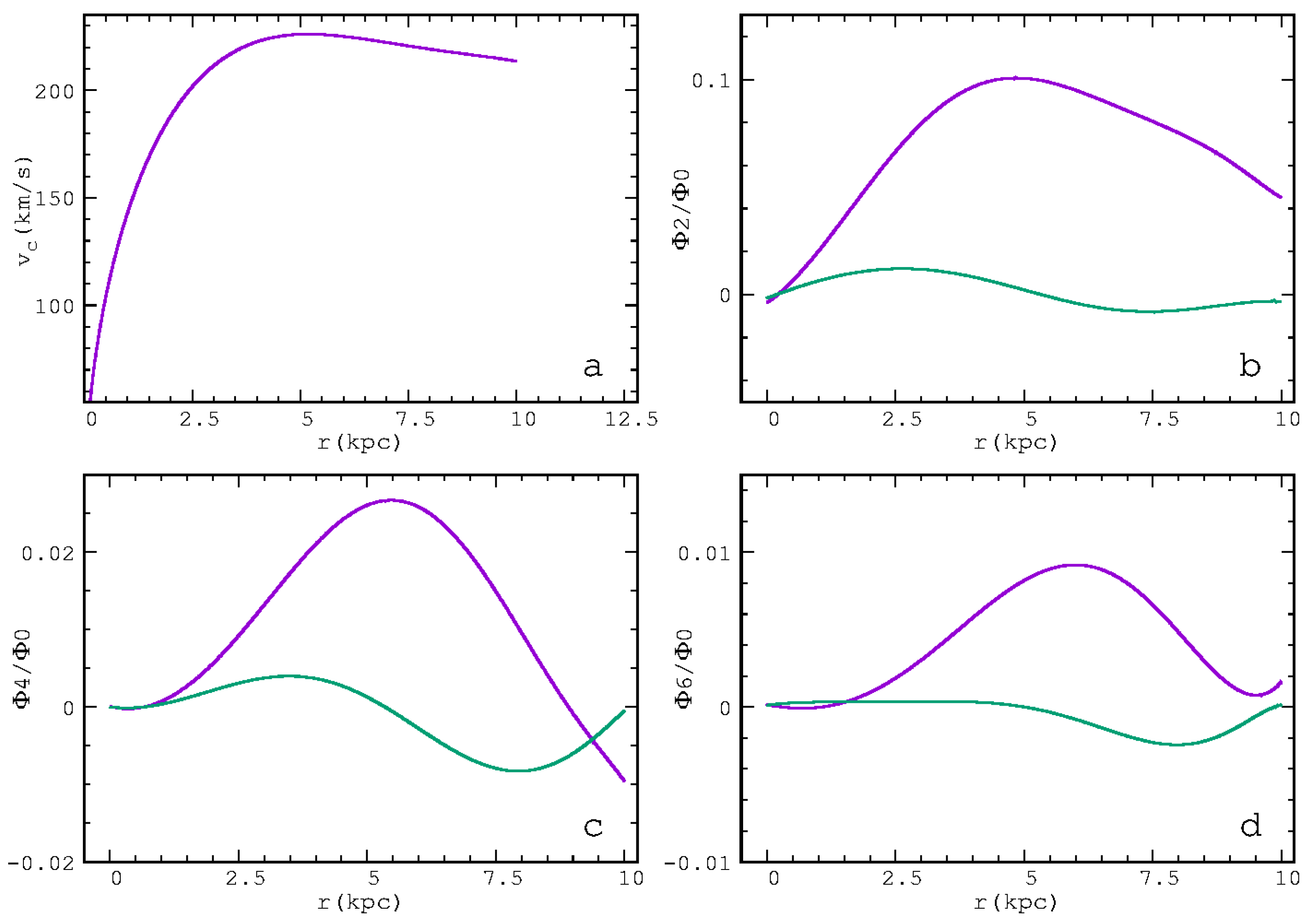
For our study, we chose a potential of the form of Equation (1), with , based on the estimation of the gravitational field of the barred galaxy NGC 7479 [10]. The adopted table with the coefficients, used in the fitting of the data with the polynomials, with , can be found in [11]. In Figure 1a, we present the rotation curve, based on the term, which is in agreement with the one given in Figure 8 in [10]. In panels b, c and d of Figure 1, we give the variation in the components of the potential, respectively, normalized by . The cosine components are plotted with magenta, while the sine ones are the green color.
As we will see in Section 3 below, this potential, rotating with a bar pattern speed , provides the orbital background against which we want to study the flow of gas. In addition, there are published studies of gaseous responses, with which we can compare our results [11,12]. In the present study, we did not try to model NGC 7479, or any particular galaxy. We, rather, investigated the flow of gas by two codes in the presence of a specific orbital background.
3. Orbital Analysis
We derived the equations of motion from the autonomous Hamiltonian
where are coordinates in a cartesian frame of reference, rotating with angular velocity (pattern speed) . Furthermore, is the potential given in Equation (1) and is the numerical value of the Jacobi constant. In the text, we will also refer to as the “energy”. Dots denote time derivatives. In all our calculations, we used the following scaling of units , kpc and km s. For the pattern speed, we adopted the value km s kpc, proposed in [11,12], as the one matching the pattern speed of NGC 7479. In our calculations, the orientation of the bar was almost along the y-axis.
3.1. Stellar Response Models
In order to understand the correspondence between the gas responses and the underlying stellar orbits in the model, we first ran a stellar response model and identified the orbits that shape its morphology.
We followed the same procedure for calculating the stellar response as the one we will follow in Section 4 for the gas models. Namely, we populated a 10 kpc disk homogeneously with particles in a circular motion in the axisymmetric part of the potential, in Equation (1), and we gradually increased the non-axisymmetric terms within a time corresponding to three pattern rotations , until we reached the full potential. Then, we continued integrating the particles for 10 pattern rotations more in the full potential. The positions and velocities of the particles at the end of the time-dependent part of the simulation were used as initial conditions for continuing their integration in the phase, during which our stellar response model behaved as an autonomous Hamiltonian system. We used a Runge–Kutta 4th-order scheme for the integration.
In Figure 2, we give eight snapshots of the stellar response. Red dots indicate the Lagrangian points of the system. Those that are close to the ends of the bar are L, the upper, and L, the lower one, at and , respectively, while those at the sides of the bar are L, to the right, and L, to the left side, at and , respectively. The snapshots are converted to images by taking into account the number density of the particles in each pixel. The corresponding pixel intensity increases from left to right, according to the (logarithmic) color bars at the bottom of the panels, which span from min = 0 to max = 25.
The successive morphologies are given in the number of pattern rotations indicated in the upper-left corners of the panels. The transient, bar-growing, phase lasts up to . In all the snapshots, there are discernible structures reminiscent of x1 POs. In Figure 2b–h, we observe a central, oval region reaching kpc. A dense straight-line feature, almost along the major axis of the bar, emerges through this oval region, reaching slightly larger distances from the center. Just outside the oval region, we can also observe loops (especially in Figure 2c,e).
Another characteristic of the stellar response model is that the region with the features identified with the x1 POs is embedded within a more extended envelope. This component reaches a kpc and a kpc. Due to its presence, we can describe the resulting morphology as composed of two “barred” structures. An inner “x1-bar” and an outer envelope of the bar. Inside the latter, we can discern some “corners” of orbits, not always at the same place (e.g., in panels Figure 2b,c), which eventually seem to be smoothed out in panels Figure 2e,f. This is a direct indication of sticky chaotic orbits [13] participating in its formation. Finally, we observe that the areas around L and L gradually become depleted of particles.
3.2. Orbits
3.2.1. Peridic Orbits (POs)
POs are periodic solutions of the system of differential equations derived from Equation (2), i.e., from the equations of motion. POs do not exist in galaxies. Nevertheless, knowledge of their location and their stability allows us to estimate the structure of the phase space in their neighborhood and, thus, assess their usefulness in supporting observed morphological structures.
A standard numerical method for finding periodic orbits in a Hamiltonian system is the Newton method (see, e.g., [14], Section 2.4.2). Since we considered the bar to be almost along the y-axis, it was more convenient to apply the Newton method by starting integrating orbits from the axis. Then, from Equation (2), we could obtain , and so the initial conditions of a PO can be defined by the coordinates .
The stability of a PO is characterized by the value of its Hénon index “” [15]. Using Hénon’s definition for this index, we see that an orbit is stable for and unstable otherwise. In the former case, the PO traps around it a set of non-periodic, “regular”, orbits reinforcing a morphology according to their topology [16]. In the latter case, the POs repel the orbits in their neighborhood and the nearby, “chaotic”, orbits can be found in a volume of phase space called a “chaotic sea”. However, chaotic orbits can be structure-supporting during a limited time period as well, if they are “sticky”, either around an island of stability, or close to the unstable asymptotic curves of unstable periodic orbits, in Poincaré cross sections [13]. Thus, the areas that support a morphological feature, such as a bar, do not overlap, in all cases, with the islands of stability we find in the Poincaré surfaces of a section [17].
Starting with a particular PO and varying continuously a parameter of the system, e.g., , we find a set of POs that we call a family [18]. The knowledge of the basic families of periodic orbits and the evolution of their stability as varies gives us the basic, essential, information for the global dynamics of a system. A useful tool for following the global dynamics of the system is the “characteristic” of a family, which is the curve that gives the initial conditions of its POs as a function of .
The characteristics of the families that play a role in the dynamics of the system we examined are given in Figure 3. The main families that play a role in the dynamics of the model are x1 and f. The main family is x1, while f is found close to 4:1 resonance. In our system, the POs have and, thus, Figure 3 is a projection of the characteristic on the plane. The green curve is the zero velocity curve (ZVC). It separates the regions where motion is allowed and we can plot the characteristics of the families from those where motion is forbidden. The location of L is indicated with a red dot in the right part of the figure.
The orbital dynamics close to the center are complicated with more families playing locally important roles. Besides x1, we encounter the family of retrograde orbits x4, as well as the x2-x3 loop with orbits, in general, perpendicular to the bar. However, in our model, they provide, along the x2-x3 loop, orbits with various inclinations with respect to the minor axis of the bar. In the embedded in Figure 3 frame, we present the projection of the characteristics of these families for in the plane. Since Figure 3 is a projection, there are orbits from different families sharing the same at an , while they differ in their initial condition. Details about the orbital dynamics in the very central region of this and other models of the general type of Equation (1) will be presented elsewhere.
The important families of POs for the present study are the following:
- The family x1. The main building block for the bar of the model is, as expected, the x1 family. However, we have to underline that, due to the presence of the sine terms in Equation (1), its orbits cross the axis with . We find that essentially all x1 orbits are cuspy and they develop loops, which are conspicuous for . Representatives of the x1 family are depicted with the black color in Figure 4a. All of them are stable, with the orbit with the largest loop and the longest projection on the y-axis being at 121,468.
- The family that we indicate as “f” in Figure 3 has a stable and an unstable part. As we observe in Figure 3, it changes its stability practically at . Orbits of this family are given in Figure 4b. The cyan- and black-colored orbits are stable at 124,157 and −120,000, respectively. The grey orbit, which has developed loops reaching the L and L regions, is at 111,723 and is unstable. As energy increases, the initial condition of the orbits of family f increases, leading to hexagonal, rhomboidal shapes. We have, in this case, along the charactristic of f in Figure 3, a transition from a 4:1 to 6:1 resonance morphology. Changes in the morphology of POs along a characteristic are observed as the curve passes through the region of a resonance (see, e.g., Figure 3.7 in [14]). For , the POs of family f are unstable. Thus, there are no stable, rectangular-like orbits, which could help the bar reach corotation. The x1 orbits at these energies already have big loops at the increasing part of the characteristic, for 121,468. They also have shorter projections on the y-axis than the outermost x1 orbit, drawn in black in Figure 4a. The situation with the orbital loops at and beyond the 4:1 resonance region is summarized in Figure 4c, where we give x1 at 121,468 (black), x1 at 112,503 (cyan) and f at 111,723 (gray).
3.2.2. Non-Periodic Orbits
The knowledge of the location and the stability of the periodic orbits provides valuable information for the dynamics of a system. Nevertheless, despite the fact that POs are the building blocks of morphological structures, their existence is practically improbable in real galaxies or even in response models such as those we present here. The orbits followed by the particles in the response model in Figure 2 belong either to some invariant curve around a stable periodic orbit in the surface of sections, or they travel in the surrounding chaotic seas.
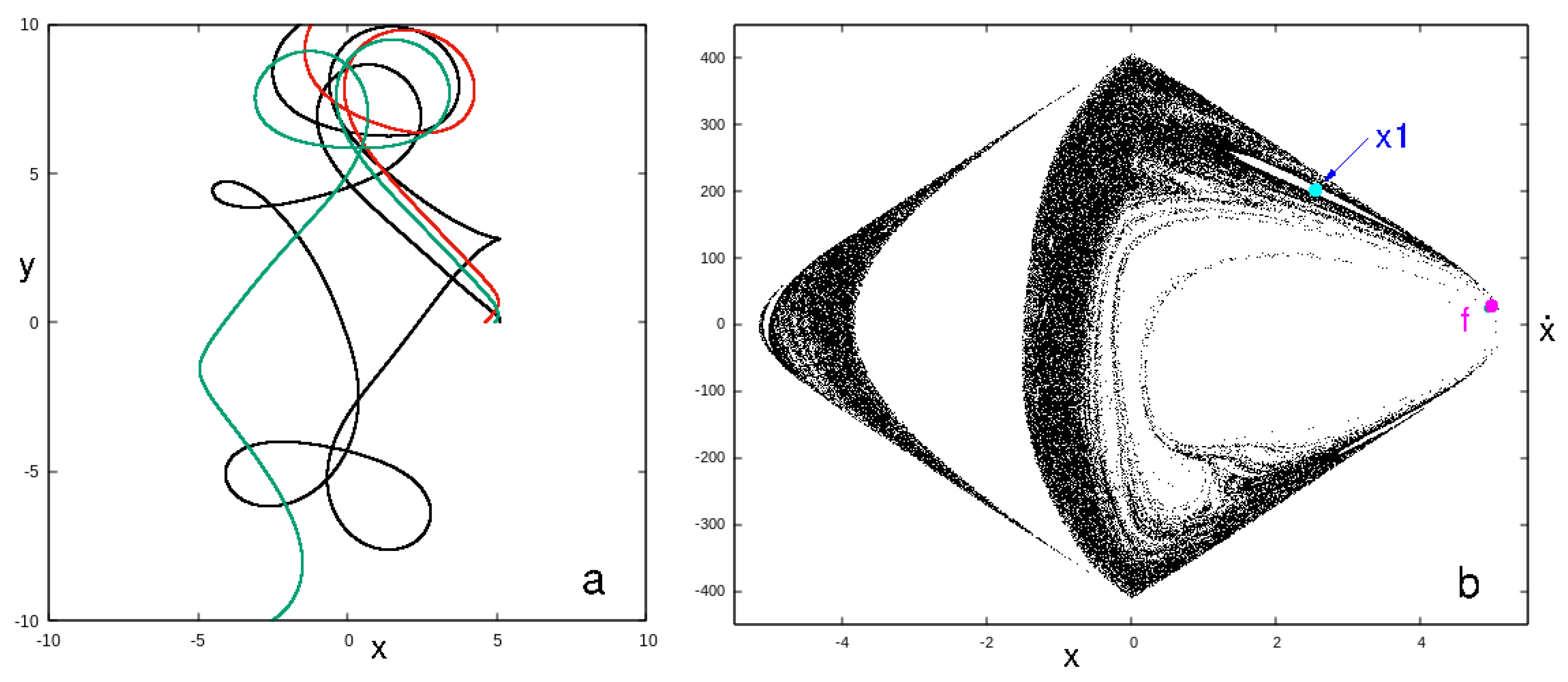
For (Figure 3), there is little space for regular motion, because the x1 stability islands are characterized by very thin and elongated invariant curves on the surfaces of the section we calculated and the f POs are unstable. Nevertheless, we find sticky zones of two kinds, namely, (a) around the x1 islands and (b) stickiness in chaos, along the unstable asymptotic curves of f [13]. Thus, non-periodic orbits at these energies will, in most cases, demonstrate a sticky behavior. This means that they will imitate quasi-periodic motion for some time and then visit the available phase space. All chaotic orbits with loops in the region of the L and L Lagrangian points will eventually cross corotation and follow retrograde motion at larger distances, in the frame of reference rotating with . A large percentage of orbits, though, visits the regions close to the unstable equilibrium points immediately and cross again the surface of section at large x, away from the bar. In Figure 5a, we give three such orbits for 111,723, while in Figure 5b, we present the central part of the surface of the section for the same energy composed by the sticky orbits of the two kinds we mentioned. The left empty area in Figure 5b, for , is occupied by (not drawn) invariant curves around the retrograde PO x4. However, the empty region at the right-hand side of the surface of the section, roughly for , is mainly due to the fact that the orbits with initial conditions in this region cross again the surface of the section at large distances, i.e., they are practically escape orbits.
Orbits sticky to the small stability islands of x1 and f for , do not cross corotation. In addition, sticky to chaos orbits associated with the unstable f orbits close beyond the transition of the family to instability, stay for long periods inside corotation. The morphology of such orbits is presented in Figure 6, which gives the f PO for (in black) and two more sticky orbits (in green and red), integrated for about three periods of f. At this energy, the f family has just become unstable and is very close to . The sticky orbits for build the component that we call the bar’s “envelope” (Figure 2g,h), which surrounds the x1 bar.
4. Gas Response
We studied the response of the gas to the barred potential of Equation (1) by means of two hydrocodes, namely, the Lagrangian scheme smoothed particle hydrodynamics (SPH) [19,20] and the adaptive mesh RAMSES code [21]. We did this in order to compare the predicted flows by means of the two codes and find possible differences due to the different derivations of the equations of hydrodynamics in the two cases.
The potential is introduced in the gas models in the same way as we described in Section 3.1 for the stellar response models. We started again from a 10 kpc disk homogeneously populated with particles in a circular motion in the axisymmetric part of the potential, and we linearly increased the bar term within three pattern rotations until its full value. The gas is not self-gravitating.
4.1. SPH
For the SPH calculations, we used the code described in [22], while test runs were performed with the SPH codes used in [23,24], obtaining practically the same results. Starting with a disk with SPH particles that play the role of tracers in order to follow the gas properties by means of the Lagrangian code, we ran a number of isothermal models with sound speeds, = 5, 10, 20 and 30 km s, combined with artificial viscosity parameters and (1, 2).
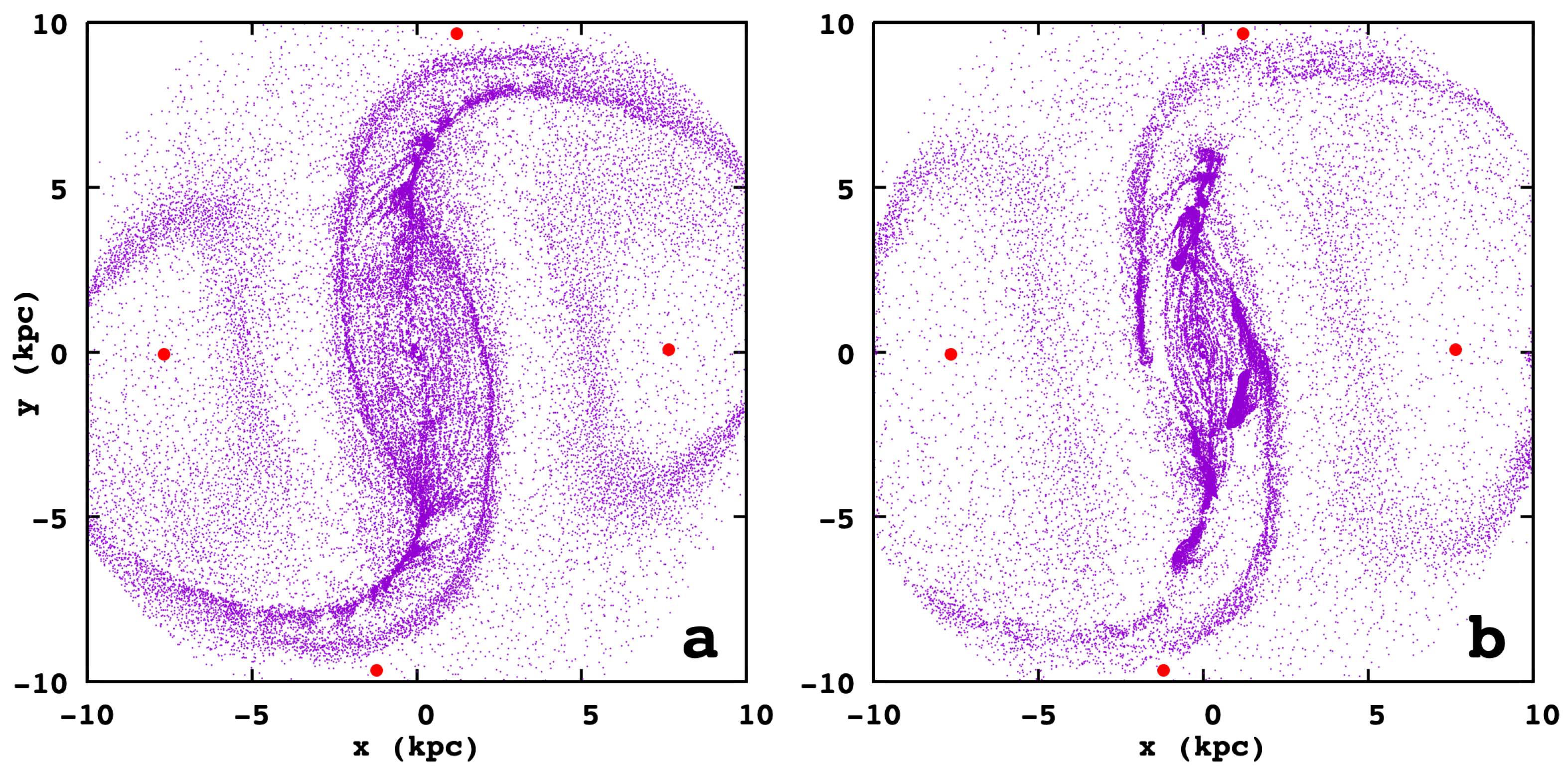
In all these models, we had a smooth response during the major part of the growing phase of the bar. However, for times close to three pattern rotations, there were already clumps formed in the high-density regions of the disk. On top of this, a considerable percentage of gaseous particles was crossing the corotation region without practically returning back to it at later times. The overall morphology during the growing phase was as in Figure 7a, while after almost three pattern rotations, as in Figure 7b. In the model of Figure 7, we have = 10 km s and . This is qualitatively in agreement with the responses found in [12] (see, e.g., their Figures 2 or 3). This is a characteristic response of this potential, independently of the hydrodynamical parameters of each individual model. We note that our calculations are in the frame of reference that rotates with km s kpc.
As time increases, the number of gaseous SPH particles is reduced. This happens because a part of them is trapped in clumps of irregular dense regions, not observed in barred galaxies in the local universe (except in some late-type galaxies) and because another part of them crosses the corotation region and practically escapes. We also observe that the regions around L and L become gradually empty. As a result, it becomes problematic to follow for a long time the evolution of the shocks and the overall morphology of the gas features in the disk. The situation improves by reducing the artificial viscosity, i.e., by using instead of (1, 2) and by increasing the sound speed of the models. Nevertheless, the improvements by varying the parameters in the response models are small. Replenishment of the “lost” particles is necessary in order to follow the evolution of the model for later times.
Replenishment of the “escaping” particles was initially applied by removing particles reaching distances larger than 11–12 kpc from the center and relocating them at random positions within a disk with a 10 kpc radius. They were given velocities corresponding to a circular motion in . Such a modification in the code was already used in the model we presented in Figure 7. However, as we can observe, the main problem remains in the over-dense regions, since these conglomerations are not dissolved with time, practically preventing the smooth formation of the dust-lane shocks in the bar region. Thus, an additional correction was necessary for preventing the trapping of particles in the spurious overdense regions. For this purpose, we considered an additional grid and a threshold of the numerical density of particles. In the various models, we tried grids ranging from to and limiting numerical densities ranging from 5 to 50 particles/cell. When the critical numerical density in a cell was exceeded, each particle had a 50% probability to be displaced in a random place in the disk, following the recipe for the “escaping” particles. This way, we avoided the formation of the irregular clumps, while we did not introduce into the model empty holes, which would have appeared if all particles of the clump were to be relocated.
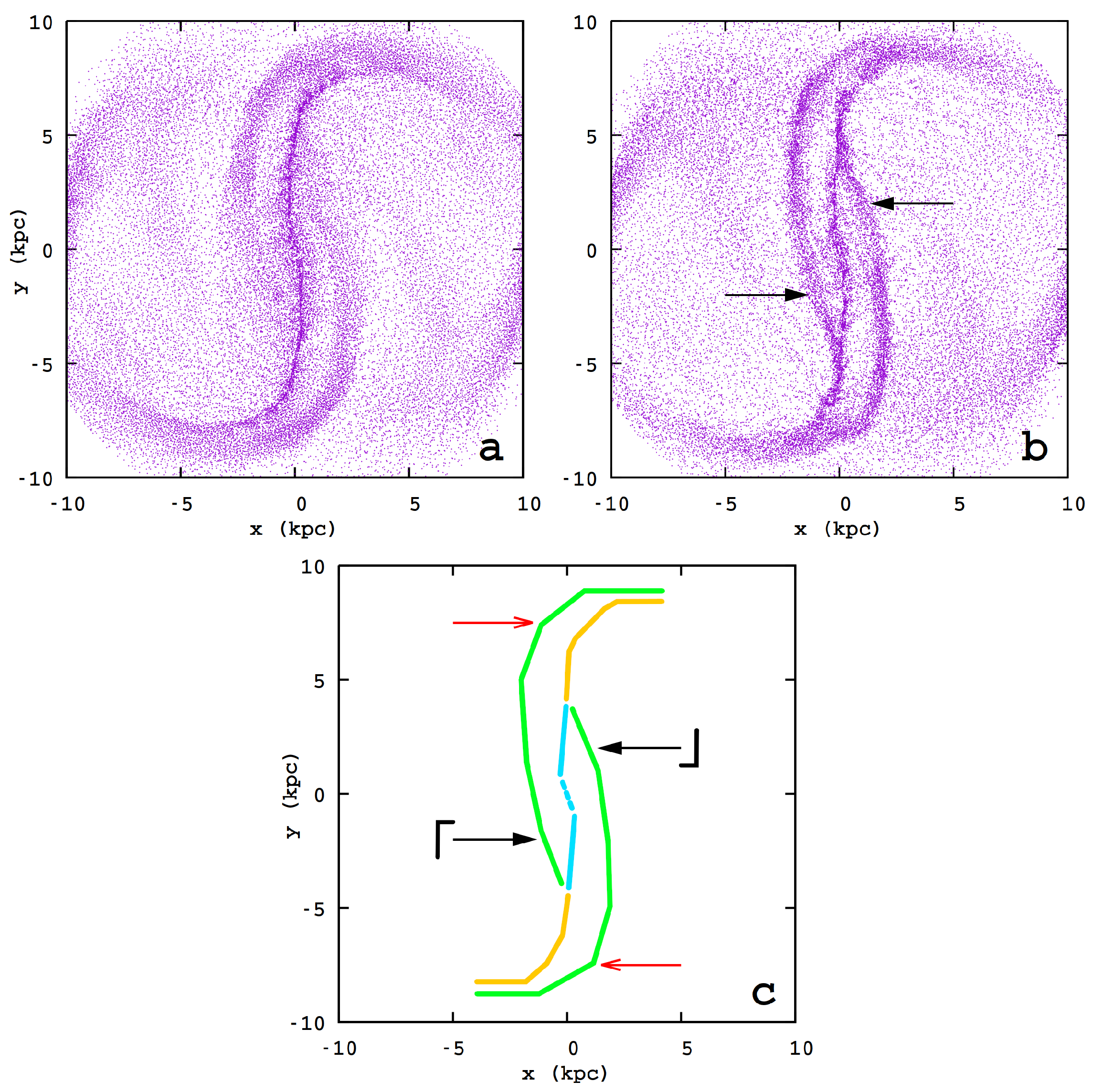
The response models could be followed then for a time as long as needed, establishing a rather invariant response morphology, as the one depicted in Figure 8, which is a typical case. In the model presented in Figure 8, we have km s, , kpc, a local grid and a critical numerical density of 40 particles/cell, for applying the redistribution of the particles. In this case, for times larger than the time when the potential has reached its final value, about 20,000 particles cross the 12 kpc radius during one bar rotation period. We stopped integrating these particles, since, in any case, the potential we used is not accurate at those distances, and we replenished the disk with an equal number of particles at random positions. In addition, in order to avoid the formation of clumps, in average 3.4 particles per step were displaced away from the over-dense regions. Let us also note that these clumps tended to be formed always at roughly the same locations.
Straight-line dust-lane shocks are typical of the response models, suggesting a strong bar [1]. In our model, they are found slightly displaced ahead of the major axis of the bar, reaching kpc. Beyond that point, they continue existing at larger distances from the center, turning eventually towards the direction opposite to the rotation of the system. In the two cases of the SPH models we presented in Figure 7 and Figure 8, the flows are qualitatively similar. In addition to the straight-line shocks, they are also characterized by the presence of elongated filament-like structures, which appear bifurcating from the straight line shocks and surround them. They are indicated with black arrows in Figure 8b. An outline of the dense regions of the response model is given in the sketch of Figure 8c. The loci of the inner part of the straight-line shocks is given in cyan and those of the outer one in yellow color. The filament-like structures are drawn in green. Due to their characteristic turn towards the trailing side of the bar, roughly beyond the points indicated with red arrows in Figure 8c, we describe them as having a “-like” morphology (“」” for the one associated to the lower part of the bar).
In Figure 9, we present the velocity field, always at the rotating with frame of reference, as it was finally developed in the snapshot of Figure 8b. Similar velocity fields were found in [1], suggesting that they are generic. Zooming into this particular region, for better understanding the details, we can follow the flow all over the disk. The critical point is A at , at the location where the green arrow points. The straight line shocks are formed below A, slightly to the left of it. Gas is flowing in the direction of rotation, upwards, in the part of the model we plot in Figure 9, is shocked and then flows down-streams ahead of the straight-line shocks. The other branch that reaches A (below and to the right of it) belongs to the feature that reaches the L region, i.e., an “」” structure (not depicted in Figure 9). It is the right “bifurcating” branch indicated with an arrow in Figure 8. We observe that the gas is flowing towards A. At the left of A, at kpc, we can see the origin of the corresponding feature reaching the bifurcating point at the lower part of the model. Gas is streaming in this region like in a funnel. We will discuss the flow in the feature again, in comparison with what we found by means of the Eulerian RAMSES scheme in Section 4.2. For the time being, we note that, according to Figure 9, the flow in the upper part of is split in two parts, one in the direction of rotation and another one in the opposite direction. The former is characterized by low velocities, which nevertheless lead the gas in the funnel of the tail of the feature. The latter is associated with the flow around L and can be traced, because of the continuous replenishment of the “lost” particles in the model. As we can see in the left part of Figure 9, the tail of is also reinforced by the flow of particles around L (not included in the figure).
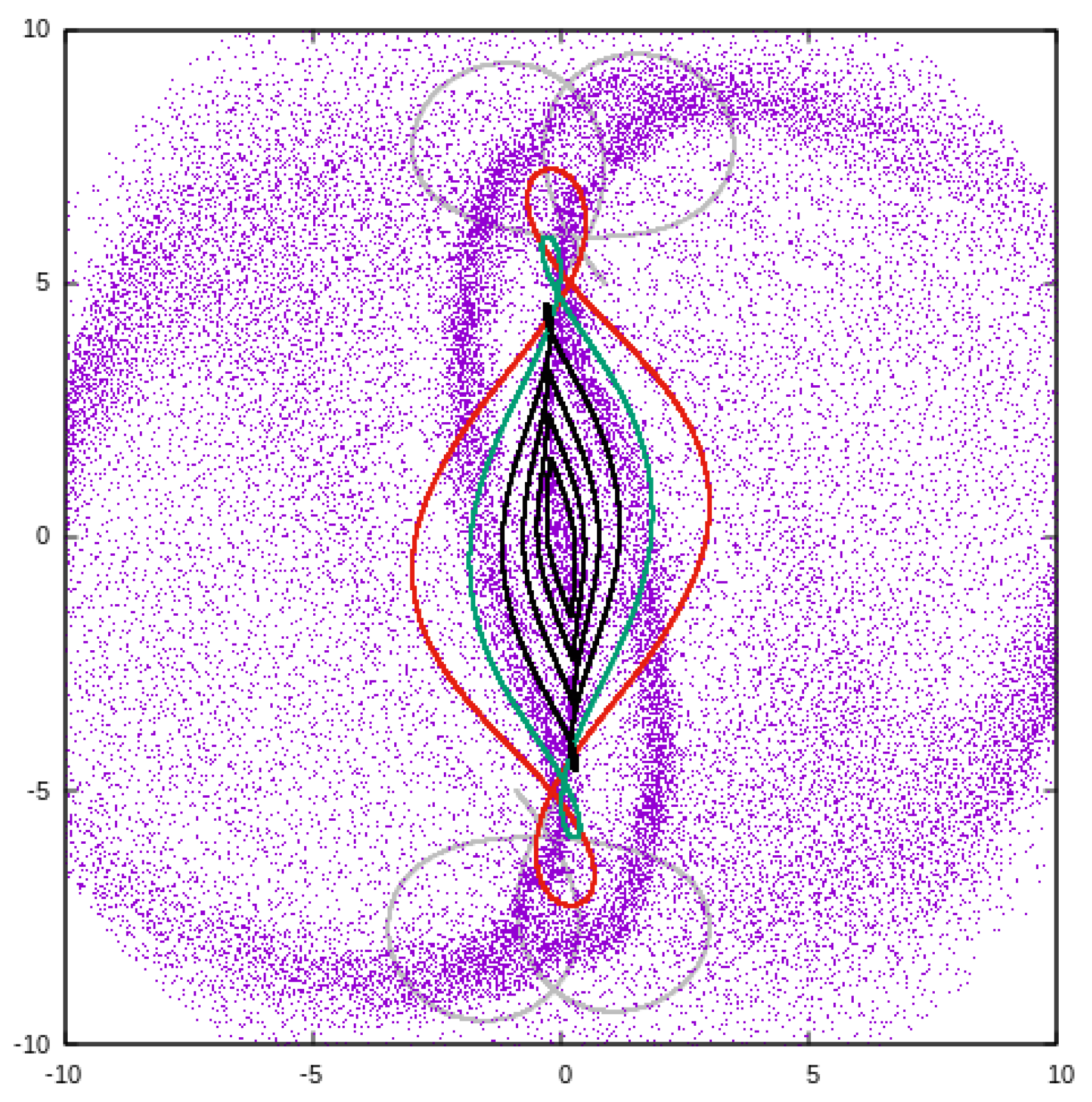
Finally, we focused on the flow of gas in the straight-line shocks region, since this is the most typical feature of hydrodynamical models in bars [1]. We find a small but evident qualitative difference in their morphology comparing snapshots during the initial growing bar phase with snapshots during the phase with the constant amplitude of the potential. This can be understood by following the gas flow in the two cases and is given in Figure 10. During the growing bar phase, the straight-line shocks are longer, with kpc, as can be seen in Figure 10a. The shocks are formed in the standard way [1], namely, as they move up stream in the direction of rotation, they are shocked along the straight-lines, loose velocity, and ahead of the shock the flow continues down stream. During the constant bar amplitude phase (Figure 10b), the straight lines hardly reach the “bifurcating” point at kpc. At larger heights, they are gradually replaced by the particles that form the tails of the feature. Their motion is opposite to the rotation of the system. Considering just the morphology of the shocks, one cannot discern the qualitative changes in the flow along the shocks. In Figure 8b, for example, the shocks close to the major axis of the bar appear along a unique curve reaching kpc. Only by careful inspection can we realize that, just beyond the point at which the tails of the bifurcating /‘」’ features appear, the shocks change inclination, becoming more perpendicular to the x-axis. In Figure 10b, we realize that this “perpendicular part” has kpc, where we can observe velocity vectors parallel to the y axis. The question that arises is what is the orbital background behind the flows described in the two last figures. In Figure 11, we plot a set of orbits over the snapshot of the SPH response model of Figure 8b. The black, green and red orbits belong to x1 and are stable. The straight-line shocks appear at the leading sides of the black x1 POs. The green one has discernible loops that appear ahead of the dense shock lanes. The red PO is the longest x1 orbit with loops, since, for larger s, the orbits of the family shrink in the y and expand in the x direction (Figure 4c) and it is not evident from Figure 2 that they are populated at all. The shocks are arranged in a such a way as to leave the major part of the loops ahead of them. On the left side of the loops, we observe that the feature also avoids the region of the loops. Finally, we plot with gray just the loops of the unstable f orbit depicted in Figure 4. It does not seem to be directly associated with the flow in the region, as it does not seem to affect the stellar flow in Figure 2.
4.2. RAMSES
In order to compare the gas responses to our potential in Lagrangian and Eulerian schemes, we used, for the latter, as earlier mentioned, the publicly available code RAMSES1 [21]. It has been successfully used in gas dynamical studies of barred and non-barred spiral galaxies [25,26]. Gas dynamics in RAMSES is computed with a second-order unsplit Godunov scheme. It is an adaptive mesh refinement scheme and in the models we present in our study, the maximum resolution used reaches 30 pc. Models with a maximum resolution of 60 pc were also used. In all cases, the gas was considered isothermal with an adiabatic index 5/3. We ran several models with sound speeds and 30 km s, as in SPH.
For test purposes, we carried out a complete study with the potential in [1], using all Ferrers models of that work having index n = 1, with the RAMSES code [27]. All responses gave identical results to the corresponding models in [1] as regards the morphology and a very similar description of the dust-lane shocks. This is important, since it confirms that any differences between the morphology of the gas flow in [1] and here will be due to the different potential and not to inadequacies of one code or another.
In all RAMSES models, we find again a typical overall response, where the main morphological features, and the corresponding flows, are the same as in SPH. Nevertheless, the details of the responses are different when different sets of the free parameters (sound speed, grid resolution, etc.) are used. A typical response is given in Figure 12, where the evolution of a model with km s and maximum resolution of 60 pc is presented. We start again with initial conditions homogeneously populating a 10 kpc disk and velocities corresponding to the circular motion in the axisymmetric part of the potential in Equation (1). As in the stellar and SPH responses, the potential grows to its full strength over three pattern rotations (we remind that km s kpc; therefore, in our time units, the rotational period is ). Thus, the flows in all cases can be compared. In addition, in this section, all figures are in the frame of reference rotating with .
In Figure 12 we give four typical snapshots. Times appear in the lower-left corner of the panels. Density increases according to the color bar are at the bottom of the figure from left (dark blue, minimum) to right (yellow, maximum). The snapshot in Figure 12a is after about two pattern rotations, i.e., still in the growing phase of the bar. The dust-lane shocks are already discernible, as well as the branches joining them at about . Towards the ends of the bar, they continue as spiral arcs with a double character. This set of double spiral arms extends mainly inside corotation (we remind that = (1.21, 9.65) and = (7.657, 0.064)). We observe that, already at this phase, we have around L low-density regions. For , these regions are found to be almost (but not completely) empty.
For times larger than (Figure 12b–d), when the bar perturbation has reached its maximum value, we observe that the straight-line, dust-lane shocks, reaching almost kpc, appear more pronounced than in Figure 12a, while the spiral arcs that appear in the upper-right and lower-left quadrants of the snapshots are fainter than during the growing bar phase. We also observe that they do not always appear as a continuation of the dust-lane shocks, as in Figure 12a. Gradually, they are transferred to -like features, similar to those developed in those SPH models at the corresponding regions of the disk (Figure 8). We note that there is a period, just after the time the bar perturbation reaches its maximum value, lasting for about , during which the model is characterized by turbulence and the formation of clumps. This is similar to the SPH models, in which we do not dissolve the over-dense regions (Figure 7b). However, in the RAMSES simulations, the clumps that formed conglomerations deform with time and gradually dissolve, without reducing their density manually. Then, the model reaches a semi-stationary phase, lasting to the end of the simulation (after at least 10 pattern rotations). The snapshots in panels Figure 12b–d are typical of the response we find.
In all panels of Figure 12, the gas is plotted on top of the stellar response (drawn in the red color) at the corresponding times. Taking into account Figure 2 and Figure 4, we realize that the stellar response in the regions of the loops is characterized by the presence of small, ansae-like features—which are formed ahead, in the direction of rotation—of the dust-lane shocks and/or their extensions.
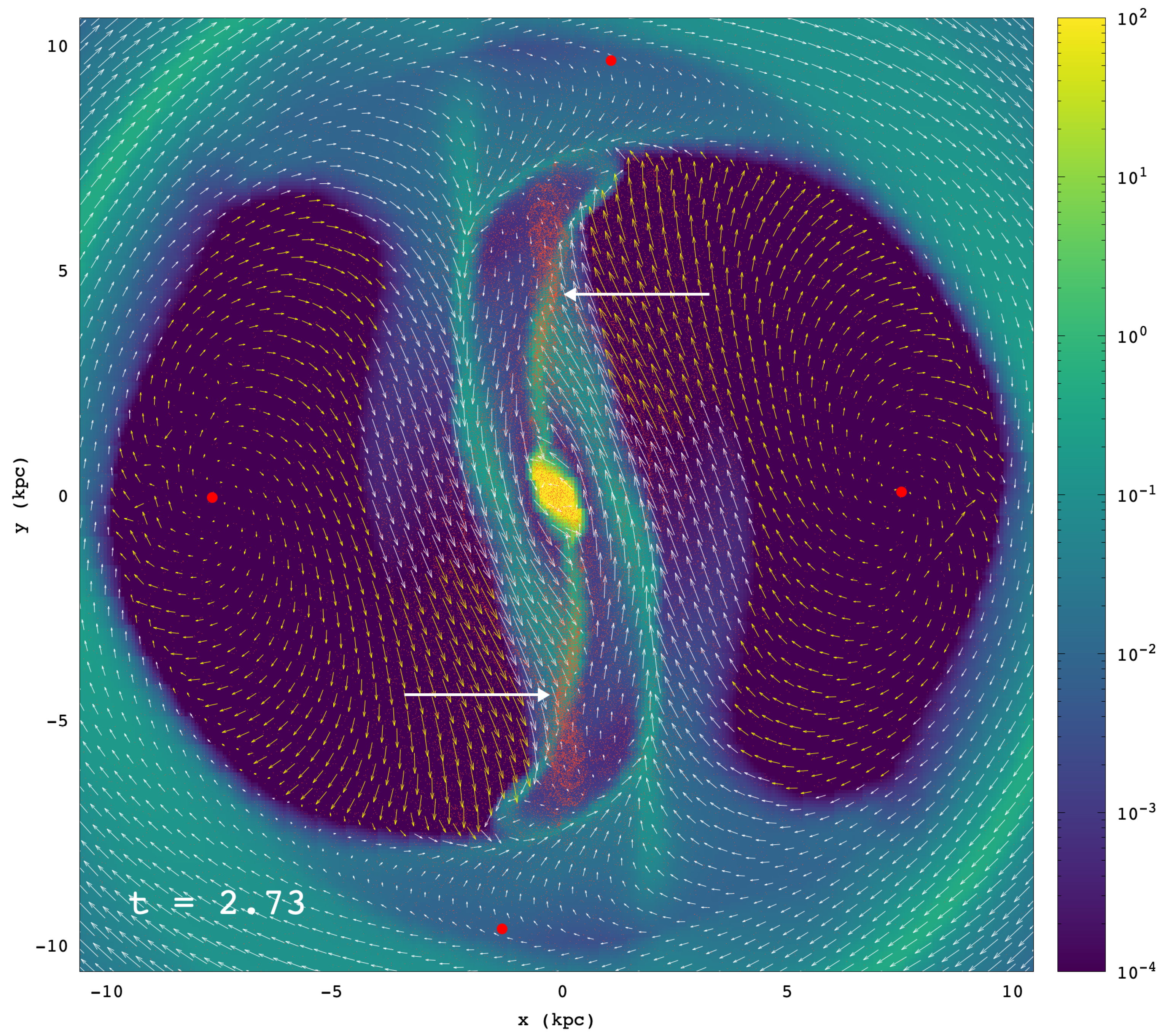
Strictly speaking, the gas morphology in the snapshots of the RAMSES responses varies with time, retaining, however, as common features the straight-line dust-lane shock loci up to kpc, the extensions bifurcating from these points, the rather-empty regions around L and L, as well as a x2 region inclined with respect to the x-axis x2 region. The last two features were also clear in [1]. These are summarized in Figure 13, which we consider as a typical RAMSES response. Breaks of the straight-line shocks are also sometimes observed, but last for very small time intervals and are reorganized again, so we may consider them as transient features. The critical points along the dust-lane shocks at which we observe the bifurcating extensions are indicated with big white arrows.
In Figure 13, we also present the overall flow of the gas, by means of the corresponding velocity arrows. Yellow arrows are used for densities below the minimum value we include in the figure, as indicated by the color bar at the right-hand side of it. Evidently, the flow in the region of the tails is toward the points where they join the shock loci. The low gas surface density regions (blue) are typical of this, as well as of all other snapshots and several previous simulation results [1]. They form one on either side of the bar. The dense parts of the shock loci, i.e., the inner straight-line parts and their curved continuations in the direction opposite to the one of the rotation of the system, avoid visiting these regions, which are occupied by quasi-periodic stellar orbits trapped around x1 POs with big loops. To show this, we give in the background of the gas in Figure 13, the stellar response model of the same time (). The stellar particles are plotted with a red color. The conspicuous reddish “bulb-like” features at the low-density gas regions, ahead of the dust-lane shocks, close to the tips of the long, white arrows, with kpc and kpc, are typical configurations built by quasi-periodic orbits associated with x1. We observe only low-density gas in transient passings through these areas, without the formation of shocks.
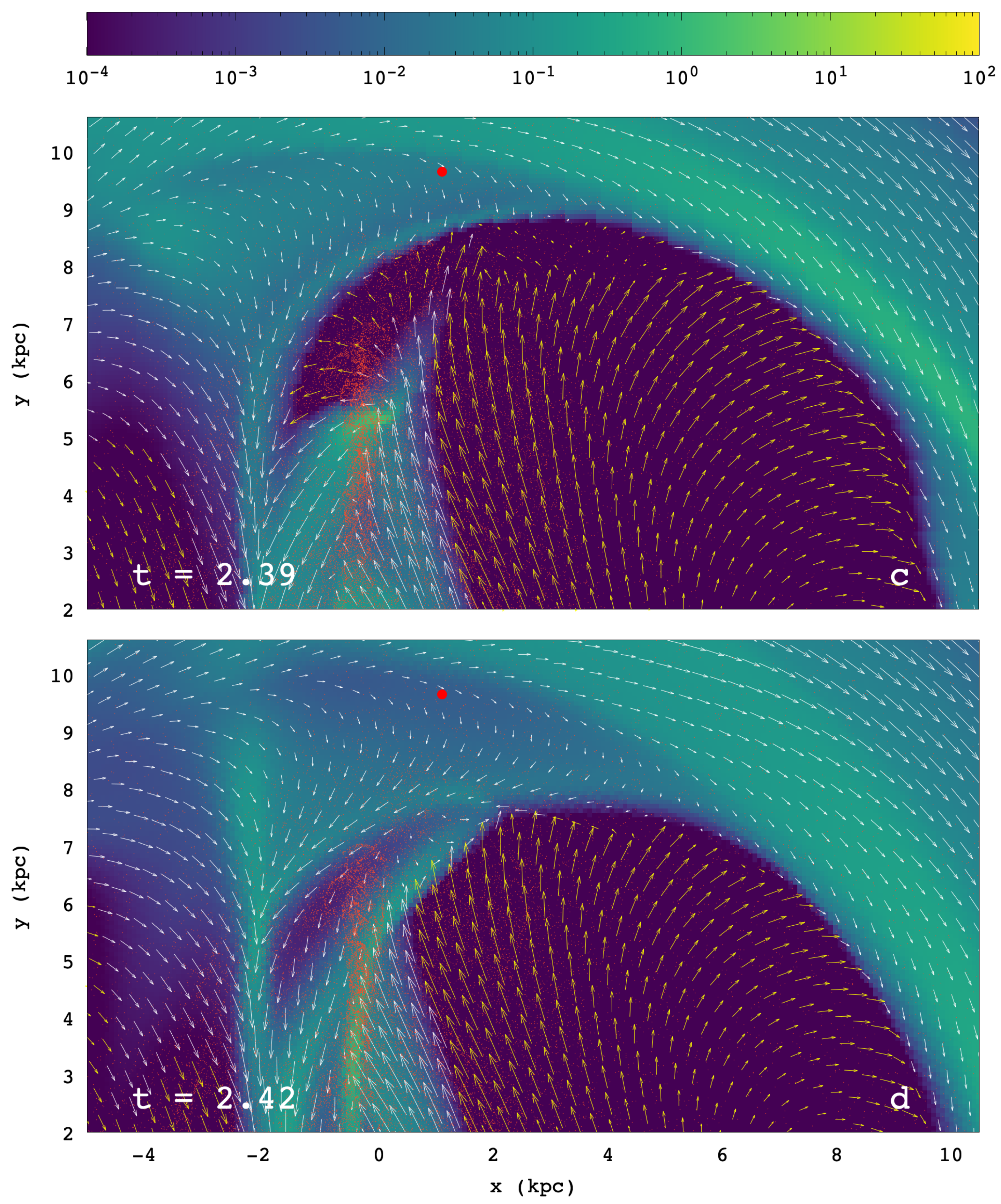
The variation of the morphologies in the RAMSES models refers mainly to the extensions of the dust-lane shocks from their straight-line part towards the -like features (their part with kpc in Figure 13) and the width of the bifurcations of the dust-lane shocks. We find that there is an approximate repeating cycle of the flow associated with the destruction and regeneration of these extensions, which also affects the rest of the gas morphology. However, during the evolution of the model up to at least 10 pattern rotations, each cycle did not have the same period as the others. In addition, during each cycle, the morphological evolution was not exactly the same. In all cases it lasted always less than T. We describe such a cycle in Figure 14, by means of four panels, during a time interval . In Figure 14a the gas streaming along the bifurcating point “A”, at kpc, indicated by a white arrow pointing to the left, bends upwards to the right, meeting the upper branch of the structure. The arrows depicting the flow point out that the gas streaming towards “A” bypasses the triangular region occupied by the big orbital loops of the test particles, colored red. The flow along the extension is from “A” to the upper branch of the structure. Then, the gas continues flowing along the denser, green regions counterclockwise, forms a loop around the rather depleted from gas triangular region and joins the flow into the “funnel” that forms the bifurcating “tail” on the left side of the bar, i.e., the side of L. This tail meets the dust-lane shock at the lower (with ) side of the bar (Figure 13). Another (heavy yellow) arrow in Figure 14a points to the location on the upper branch of “”, at which the flow “splits”, pointing to two opposite directions. We remind that all these features are inside corotation. The flow along the “chaotic” spirals is above and to the right of the heavy, yellow arrow and is associated with the clockwise pointing arrows of the flow.
In Figure 14b, the streaming along the bifurcating tail towards “A” is accumulated at the upper end of the dust-lane shock, forming a characteristic bending of it to the right. The extension above this point towards the upper branch of the feature is not observed.
The flow of the gas, as given by the arrows, indicates a weak extension, not discernible at the level of densities chosen for presenting the flow. Low-density gas, now from a broader area, is streaming into the region ahead of the dust-lane shocks. The upper branch of the is shifted to larger distances from the center and the point along it, at which the flow “splits”, has moved to the left, compared with Figure 14a (again indicated with a heavy, yellow arrow). At a certain time, the accumulated gas conglomeration at the end of the x1-dust -lane shock recedes, as gas along the bifurcating tail continues streaming towards “A”. Then, the accumulated gas starts flowing upwards, bypassing the region where the underlying test particle orbits form loops (Figure 14c). Finally, in Figure 14d, we reach a situation similar to the one encountered in Figure 14a, with the gas flowing around the triangular, low gas density region, occupied by the orbital loops.
As we mentioned before, the cycles are not identical and, while being relatively short-lived, do not evidently have a specific period. In order to find a mean response for our RAMSES model, we considered 100 snapshots for the period , i.e., during the time we have a quasi-stationary response. This period corresponds to 4.35 rotational periods of the system. We stacked the images of all these snapshots and the result can be seen in Figure 15. The result resembles the typical response we presented in Figure 13, both as regards the average morphology as well as the average flow, which is given in enlargement in the upper-right corner of the figure.
The overall response does not change as the sound speed, , varies. However, there are several differences in the details. We followed the responses of the same initial conditions in models with the same resolution but with different . In Figure 16a, we give the response in a model with , while in Figure 16b, a model with 20 km s. There are no major differences between the model in Figure 16a and the model with km s in Figure 12. However, as increases, differences in the models come into view: more conspicuous are the instabilities that appear along the extensions towards the upper part of the structures, i.e., in regions with strong density gradients. In addition, the contrast between low- and high-density regions decreases. For example, in the regions around L and L in Figure 16b, we encounter gas diffusing, increasing this way the gas density compared with the snapshots of models with lower sound speed at the same time. For even larger ’s, these instabilities are more evident.
5. Discussion
5.1. Code Dependence of the Responses
In our study, the equations of hydrodynamics were first derived in Lagrangian (co-moving) form, where the coordinate system is attached to moving mass elements, and then in Eulerian form, where the coordinate system is fixed in space. The corresponding codes used were versions of the SPH and RAMSES schemes, respectively.
Responses with both codes gave results with some common, main morphological features. These are: 1. The dust-lane shocks in the bar region, 2. the tails that are attached to them at the end of the straight-line part of the dust-lane shocks (indicated with arrows in Figure 13 and Figure 14a), 3. the -like features formed by these tails together with their extensions backwards with respect to the rotation of the system, and 4. the inclined “x2” region in the central part of the bar.
Nevertheless, there are several differences as well. They can be summarized by comparing Figure 8 with Figure 15. Besides the different modeling techniques, we remind that, in SPH, we are removing from the simulation the gas particles that are found to be practically in escape trajectories, as well as half of the particles that are trapped in over-dense regions. The removed SPH particles were replenished by an equal number of particles placed randomly on the disk, with velocities corresponding to the circular velocity in the axisymmetric part of the potential. This was essential, because it allowed us to continue with a meaningful simulation at larger times. Nothing similar was needed for the RAMSES simulations. On one hand, the SPH responses with the replenishment of the removed particles lead to more stationary models; on the other hand, the RAMSES results are more objective.
The most characteristic difference of the RAMSES snapshots compared with SPH is the continuous displacement of the morphological features on the disk, mainly outside the bar region, something that leads to a cycle of the flow rather than to a stationary morphology. Nevertheless, there is a mean RAMSES morphology with clearly shaped structures (Figure 15). This mean snapshot and the corresponding mean flow are qualitatively similar with what we find in the SPH responses. Finally, another conspicuous difference is the low-density regions around L and L appearing in the RAMSES snapshots, mainly for . This is not observed in the SPH models, due to the continuous replenishment of particles we applied (see also Section 5.2 below).
5.2. Stellar vs. Gas Response
In both modeling techniques, there is a direct relation between the underlying orbital structure and the gaseous responses, and this relation is the same for the response models of both the SPH and RAMSES codes. Namely, the straight-line dust-lane shocks are formed in the region where the x1 POs are elliptical-like with cusps (or tiny loops). In the particular potential we studied, these are x1 POs with projections on the y axis of the system, reaching kpc. Due to the presence of the sine terms in the potential (Equation (1)), the x1 orbits slightly precess, facilitating, due to their orientation, the straight-line, dust-lane-shock formation (Figure 4a).
At larger distances from the center of the bar, the POs of this family develop loops of considerable size (Figure 11). This is a direct indication that the bar of the model is strong [2,28]. As soon as the POs of x1 develop conspicuous loops at their apocenters, the local density maxima of the gas are formed away from the x1-orbital flow. As the gas bypasses the x1 loops, it creates extensions of the dust-lane shocks, in general at an angle with them, in the direction away from the major axis of the bar.
The patterns that we call “tails” or “bifurcations of the dust-lane shocks” (indicated with arrows, e.g., in Figure 8b) appear at the sides of the bar. They are formed at the region where the “banana-like” flow around L and L meets the orbits of the f family. The dimensions of the longest rectangular-like, stable f POs marginally match the dimensions of a structure that can be vaguely described as boxy, formed essentially by two symmetric, with respect to the center of the system, -like features (/」) (see, e.g., Figure 7 and Figure 13).
As we can see in Figure 2, the stellar bar, including its rectangular-like “chaotic” envelope as well, reaches a maximum 8.5 kpc. This length coincides more or less with the y at which we observe the “horizontal”, roughly parallel to the x axis, branch of the feature (Figure 15). In smaller radii from the center, we notice that the straight-line, dust-lane shocks, reach distances 4.5–5 kpc. In the zone kpc, we have the x1 POs with loops and the orbits of the f family. However, the orbits of the f family, which reach distances 6–7 kpc from the center, are unstable and, at even larger energies, they obtain 6:1 type morphologies with loops (Figure 4b). They are characterized by sticky regions around them and along their unstable asymptotic curves (Figure 5). An issue that needs further investigation is whether the shape of the extensions of the dust-lane shocks in the kpc zone and the formation of the “horizontal” branch of the ’s are determined just by the presence of the loops of the x1 orbits or if the asymptotic curves of the manifolds of the underlying unstable POs also play a role.
The resulting morphologies are established essentially at the end of the growing phase of the bar that lasts for three rotational periods of the system. Numerical problems, such as the overdense clumps in SPH, or the transient “turbulent” phase in RAMSES, occur close to the end of this period. Although the models survive in one or the other to longer times, understanding the smooth responses during the growing phase of the models remains an open question. Is it due to the growing character of the perturbation, or because the final amplitude of the model is large for real galaxies? In the latter case, response models could be used for estimating M/L ratios in near-infrared images of real galaxies.
Another interesting feature of the models is the low density in the regions of L and L at the sides of the bar. This is in agreement with the rather empty regions of the stellar responses and the fact that, for the ’s at which the banana-like orbits around L and L exist, non-periodic orbits are not trapped around them. They visit the neighborhood of L, L and then cross corotation. Such a behavior in SPH models with unstable POs around L and L has already been found in a series of models in [29]. The overall dynamics of the present case is consistent with the flows of those models.
The instability of the banana-like and f orbits, in a considerable range, is typical for models with large bar perturbations. If we let the amplitude of the perturbation grow within to 50% of the maximum value used so far and then follow the response up to , stellar and gaseous responses change. The result is presented in Figure 17 and the differences with the corresponding stellar (cf. Figure 17a with Figure 2) and gaseous (cf. Figure 17b with Figure 15) responses are conspicuous. The disks with the initial conditions are homogenously populated, so it is evident that, in the case of Figure 17a, non-periodic orbits are now trapped around L and L and the gas density at the corresponding regions of Figure 17b are considerably larger than what we find in Figure 15. The L and L regions resemble those that are found in several models of specific barred galaxies [30]. In addition, elliptical-like orbits reinforce a bar up to 7 kpc in Figure 17a, while at the same region in Figure 17b we can observe a thick ring structure reaching this distance. The overall response in the bar region resembles the models in Sormani et al. [31].
In the present paper, we do not attempt to compare our models with features of specific galaxies, despite the fact that the model is the result of the estimation of a specific barred-spiral galaxy (NGC 7479). A systematic comparison of morphological features and of the form of dust lanes, with images of barred-spiral galaxies and the comparison of the associated velocity fields, will give valuable information about the underlying stellar orbital structure, the pattern speeds of the bars and the spirals, or even about the mass-to-light ratios on the disks, as has been performed in [26]. This work is in progress.
6. Conclusions
- The basic conclusion of the present study is that the dust-lane shocks in the gas responses of barred galaxies models avoid the regions in which the stable POs of the x1 family have developed sufficiently big loops. They deviate from these regions and, as they bypass them, they form extensions at an angle with the straight-line shocks. Ahead of them, in the direction of rotation, we find low-density regions, which in many cases have a “triangular”-like shape, as, e.g., model 12 in [1]. This morphology is encountered in both codes we used (SPH and RAMSES).
- Responses during the growing-bar phase are smoother, in the sense that we observe fewer regions with strong density gradients. As the amplitude of the perturbation during this phase is always smaller than the final, maximum one, the models do not develop x1 POs with big loops (Figure 2a). Thus, the straight-line, dust -lane shocks extend to larger distances.
- A characteristic feature of the models are the “tails”, which are dense regions that appear bifurcating from the straight dust-lane shocks at specific points along them. The bifurcating points are identified with the points at which the x1 POs start having considerable loops (indicated with arrows in Figure 8). Gas is streaming along these lanes towards the points where the three density enhancement join.
- The SPH models can be followed for a long time only with replenishment of particles that are manually removed mainly from the overdense regions, but it gives, after a certain time, an invariant response. RAMSES, on the other hand, has a short, relatively turbulent phase for and then reaches a repeating cycle, where the morphology of the straight-line dust-lane shocks and their extensions characterize the snapshots. Nevertheless, there is a dominating “mean” morphology, given in Figure 15.
- Both codes give information valuable for understanding the dynamics of the model and should be used when comparison with the morphology of specific galaxies is attempted. With the Lagrangian SPH method, we can obtain detailed velocity fields in the the dense regions of the model, while with the grid code RAMSES, we can obtain an overall picture of the kinematics of the models. Both modeling techniques are useful for understanding gas dynamics in barred-spiral galaxies.
- Finally, as regards the stellar response, in this model, like in the case of the models for NGC 4314 we studied in [6] and for NGC 1300 in [9], we find a second bar, which is a “chaotic” envelope around the x1 bar. It is “chaotic”, in the sense that it is supported by chaotic orbits. The consistency of its appearance in the models indicates that this is rather a common feature in barred galaxies.
Author Contributions
Conceptualization, methodology, P.A.P. and E.A.; writing—original draft preparation, S.P. and P.A.P.; writing—review and editing, all authors; software and validation, S.P.; formal analysis, S.P.; data curation, S.P.; visualization, S.P.; supervision, P.A.P. and E.A.; project administration, P.A.P. All authors have read and agreed to the published version of the manuscript.
Funding
This research received no external funding.
Institutional Review Board Statement
Not applicable.
Informed Consent Statement
Not applicable.
Data Availability Statement
The data underlying this article will be shared on reasonable request to the corresponding author.
Conflicts of Interest
The authors declare no conflict of interest.
Abbreviations
The following abbreviations are used in this manuscript:
| PO(s) | Periodic orbit(s) |
| SPH | Smoothed particle hydrodynamics |
| 1 | Available in https://bitbucket.org/rteyssie/ramses/src/master/, accessed on 16 May 2022. |
References
- Athanassoula, E. The existence and shapes of dust lanes in galactic bars. Mon. Not. R. Astron. Soc. 1992, 259, 345–364. [Google Scholar] [CrossRef]
- Athanassoula, E. Morphology of bar orbits. Mon. Not. R. Astron. Soc. 1992, 259, 328–344. [Google Scholar] [CrossRef] [Green Version]
- Quillen, A.C.; Frogel, J.A.; Gonzalez, R. The Gravitational Potential of the Bar in NGC 4314. Astrophys. J. 1994, 437, 162–172. [Google Scholar] [CrossRef]
- Boonyasait, V. Structures and Dynamics of NGC 3359: Observational and Theoretical Studies of a Barred Spiral Galaxy. Ph.D. Thesis, University of Florida, Gainesville, FL, USA, 2003. [Google Scholar]
- Kalapotharakos, C.; Patsis, P.A.; Grosbøl, P. NGC 1300 dynamics–I. The gravitational potential as a tool for detailed stellar dynamics. Mon. Not. R. Astron. Soc. 2010, 403, 83–95. [Google Scholar] [CrossRef] [Green Version]
- Patsis, P.A.; Athanassoula, E.; Quillen, A. Orbits in the Bar of NGC 4314. Astrophys. J. 1997, 483, 731–744. [Google Scholar] [CrossRef] [Green Version]
- Patsis, P.A.; Kaufmann, D.E.; Gottesman, S.T.; Boonyasait, V. Stellar and gas dynamics of late-type barred-spiral galaxies: NGC 3359, a test case. Mon. Not. R. Astron. Soc. 2009, 394, 142–156. [Google Scholar] [CrossRef] [Green Version]
- Tsigaridi, L.; Patsis, P.A. The backbones of stellar structures in barred-spiral models–The concerted action of various dynamical mechanisms on galactic discs. Mon. Not. R. Astron. Soc. 2013, 434, 2922–2939. [Google Scholar] [CrossRef] [Green Version]
- Patsis, P.A.; Kalapotharakos, C.; Grosbøl, P. NGC1300 dynamics—III. Orbital analysis. Orbital analysis. Mon. Not. R. Astron. Soc. 2010, 408, 22–39. [Google Scholar] [CrossRef] [Green Version]
- Quillen, A.C.; Frogel, J.A.; Kenney, J.D.P.; Pogge, R.W.; Depoy, D.L. An Estimate of the Gas Inflow Rate along the Bar in NGC 7479. Astrophys. J. 1995, 441, 549–560. [Google Scholar] [CrossRef] [Green Version]
- Laine, S. Observations and Modeling of the Gas Dynamics of the Barred Spiral Galaxy NGC 7479. Ph.D. Thesis, University of Florida, Gainesville, FL, USA, 1996. [Google Scholar]
- Laine, S.; Shlosman, I.; Heller, C.H. Pattern speed of the stellar bar in NGC 7479. Mon. Not. R. Astron. Soc. 1998, 297, 1052–1059. [Google Scholar] [CrossRef] [Green Version]
- Contopoulos, G.; Harsoula, M. Stickiness in Chaos. Int. J. Bif. Chaos 2008, 18, 2929–2949. [Google Scholar] [CrossRef] [Green Version]
- Contopoulos, G. Order and Chaos in Dynamical Astronomy; Springer: Berlin/Heidelberg, Germany, 2002. [Google Scholar]
- Hénon, M. Exploration numérique du problème restreint. II. Masses égales, stabilité des orbites. Ann. d’Astrophys. 1965, 28, 992–1007. [Google Scholar]
- Patsis, P.A. On the relation between orbital structure and observed bar morphology. Mon. Not. R. Astron. Soc. 2005, 358, 305–315. [Google Scholar] [CrossRef] [Green Version]
- Chatzopoulos, S.; Patsis, P.A.; Boily, C.M. A taxonomic algorithm for bar-building orbits. Mon. Not. R. Astron. Soc. 2011, 416, 479–492. [Google Scholar] [CrossRef] [Green Version]
- Poincaré, H. Les Méthodes Nouvelles de la Mécanique Céleste; Gauthier Villars: Paris, France, 1892. [Google Scholar]
- Gingold, R.A.; Monaghan, J.J. Smoothed particle hydrodynamics: Theory and application to non-spherical stars. Mon. Not. R. Astron. Soc. 1977, 181, 375–389. [Google Scholar] [CrossRef]
- Lucy, L.B. A numerical approach to the testing of the fission hypothesis. Astrophys. J. 1977, 82, 1013–1024. [Google Scholar] [CrossRef]
- Teyssier, R. Cosmological hydrodynamics with adaptive mesh refinement. A new high resolution code called RAMSES. Astron. Astrophys. 2002, 385, 337–364. [Google Scholar] [CrossRef] [Green Version]
- Patsis, P.A.; Athanassoula, E. SPH simulations of gas flow in barred galaxies. Effect of hydrodynamical and numerical parameters. Mon. Not. R. Astron. Soc. 2000, 358, 45–56. [Google Scholar]
- Bate, M.R.; Bonnell, I.A.; Price, N.M. Modelling accretion in protobinary systems. Mon. Not. R. Astron. Soc. 1995, 277, 362–376. [Google Scholar] [CrossRef]
- Kitsionas, S.; Whitworth, A.P. Smoothed Particle Hydrodynamics with particle splitting, applied to self-gravitating collapse. Mon. Not. R. Astron. Soc. 2002, 330, 129–136. [Google Scholar] [CrossRef] [Green Version]
- Few, C.G.; Dobbs, C.; Pettitt, A.; Konstandin, L. Testing hydrodynamics schemes in galaxy disc simulations. Mon. Not. R. Astron. Soc. 2016, 460, 4382–4396. [Google Scholar] [CrossRef] [Green Version]
- Fragkoudi, F.; Athanassoula, E.; Bosma, A. Constraining the dark matter content of NGC 1291 using hydrodynamic gas response simulations. Mon. Not. R. Astron. Soc. 2016, 466, 474–488. [Google Scholar] [CrossRef] [Green Version]
- Pastras, S. Comparing Hydrodynamics Codes for Modeling the Gas Flow in Barred Spiral Galaxies. Master’s Thesis, University of Athens, Athens, Greece, 2022. [Google Scholar]
- Contopoulos, G. The 4: 1 resonance in barred galaxies. Astron. Astrophys. 1988, 201, 44–50. [Google Scholar]
- Patsis, P.A.; Tsigaridi, L. The flow in the spiral arms of slowly rotating bar-spiral models. Astrophys. Space Sci. 2017, 362, 129–135. [Google Scholar] [CrossRef]
- Treuthardt, P.; Seigar, M.S.; Sierra, S.; Al-Baidhany, I.; Salo, H.; Kennefick, D.; Kennefick, J.; Lacy, C.H.S. On the link between central black holes, bar dynamics and dark matter haloes in spiral galaxies. Mon. Not. R. Astron. Soc. 2012, 423, 3118–3133. [Google Scholar] [CrossRef] [Green Version]
- Sormani, M.C.; Binney, J.; Magorrian, J. Gas flow in barred potentials. Mon. Not. R. Astron. Soc. 2015, 449, 2421–2435. [Google Scholar] [CrossRef] [Green Version]
Figure 1.
The circular speed (a) and the k = 2 (b), k = 4 (c) and k = 6 (d) components of the potential, normalized by , as a function of the radius r. From (b–d), magenta curves refer to the cosine and green to the sine terms.
Figure 1.
The circular speed (a) and the k = 2 (b), k = 4 (c) and k = 6 (d) components of the potential, normalized by , as a function of the radius r. From (b–d), magenta curves refer to the cosine and green to the sine terms.

Figure 2.
(a–h) Successive snapshots of the stellar response model. Lighter regions correspond to denser regions, according to the logarithmic color bar at the bottom of the panels. The number of pattern rotations is given at the upper-left corner of the frames. The red dots indicate the location of L (top), L (bottom), L (right) and L (left) of the bar. The bar rotates counterclockwise.

Figure 3.
Characteristics of the main families of POs, x1 and f, projected in the (, ) plane. Stable parts of these curves are plotted with black, while unstable with red, color. The zero-velocity curve is the thick green curve, having at its local maximum the L point. The area between the ’s of L and L is shaded with cyan color. In the embedded frame, we give an enlargement of the characteristics of all main families close to the center of the system (see text). The x2-x3 loop is plotted with magenta, the x1 characteristic with balck and that of x4 with blue color.

Figure 4.
Periodic orbits with loops. (a) Stable orbits of x1 are plotted with black and an unstable f with pairs of loops at its apocenters is plotted with grey. (b) Two stable f orbits (black and cyan) and an unstable in grey. (c) POs with loops beyond the 4:1 resonance. The grey belongs to f, while the two others (black and cyan) to x1.

Figure 5.
(a) Three orbits with loops, plotted with black, green and red color) that follow different paths and eventually cross the corotation region . (b) The central part of the surface of section at 111,723. The location of x1 and f are indicated with a green and magenta dot, respectively. The left empty part (roughly for ) is occupied by invariant curves around x4 (not plotted), while the empty part for is due to the fact that orbits with initial conditions in this region are practically escape orbits (they intersect the surface of section at large distances, outside the frame of panel).

Figure 6.
The f PO for 118,092 (in black) together with two sticky periodic orbits (red and green) at the same energy, integrated for about three periods of f. The orbits do not reach the unstable Lagrangian points, located at .
Figure 6.
The f PO for 118,092 (in black) together with two sticky periodic orbits (red and green) at the same energy, integrated for about three periods of f. The orbits do not reach the unstable Lagrangian points, located at .

Figure 7.
The SPH response without redistribution of the particles, during the growing phase of the bar, for (a) and for (b). The artificial viscosity parameters we used are . In this, and in all relevant subsequent figures, the bar rotates counterclockwise. Red dots indicate the Lagrangian points of the model.

Figure 8.
Characteristic snapshots of a typical model with redistribution of particles in action, at (a) and (b). In (c) we give a sketch that outlines the dense parts of the model. In the text, the green features, indicated with arrows, are described as “/」”. We draw the straight-line dust lane shocks and its continuations with cyan and yellow color respectively.

Figure 9.
The velocity field of the snapshot of Figure 8 is given by zooming into its region. The green arrow indicates point A, where the tail of the lower feature joins the straight-line shocks. The green dot at indicates the location of L.
Figure 9.
The velocity field of the snapshot of Figure 8 is given by zooming into its region. The green arrow indicates point A, where the tail of the lower feature joins the straight-line shocks. The green dot at indicates the location of L.

Figure 10.
The flow in the straight-line shocks region in two typical cases. (a) During the growing bar phase. (b) During the time the bar has a constant amplitude . We can observe in (b) how the particles of the bifurcating tail help the shock extend to larger distances from the center, as they flow upwards in the direction opposite to the rotation of the system.

Figure 11.
Stable x1 orbits (black, green and red) and the (grey) loops of an 6:1 f orbit (see Figure 4). The straight-line shocks are formed in the region occupied by the black x1 POs. The shocks avoid the loops, while the unstable f orbit does not affect the flow.
Figure 11.
Stable x1 orbits (black, green and red) and the (grey) loops of an 6:1 f orbit (see Figure 4). The straight-line shocks are formed in the region occupied by the black x1 POs. The shocks avoid the loops, while the unstable f orbit does not affect the flow.

Figure 12.
The evolution of a typical RAMSES model, with km s . The snapshot in (a) is in the growing bar phase, while in (b–d) the bar perturbation has already reached its maximum. Times are given in the lower-left corner of the frames. Densities increase from left to right according to the logarithmic scale of the color bar at the bottom of the figure. In red, we plot the stellar response particles at the corresponding times. The bar rotates counterclockwise. Red dots indicate the location of the Lagrangian points.

Figure 13.
A typical snapshot of our RAMSES simulation, summarizing the main morphological features, together with the velocity vectors indicating the flow. The flow vectors are colored yellow, when they are in regions below the minimum density we considered. The two long white arrows indicate the point where the tails of the features join the dust-lane shocks in the bar region. The stellar response is given in the background using a red color for the test particles.

Figure 14.
(a–d): Characteristic evolution of the flow at the end and beyond the x1-bar region within a period, during which the extension towards the -like feature breaks and forms again. Times are given at the lower left corner of the panels. The flow in the upper branch of the feature splits, pointing to two opposite directions at the points indicated with heavy yellow arrows in (a,b). The long white arrow in (a) indicates the point “A”, where the tail of the 」 feature join the dust-lane shock in the bar region. Red dots mark the location of L.


Figure 15.
A mean RAMSES response morphology, created by stacking the images of 100 snapshots within 4.35 rotational periods of the system. It has all the typical morphological features discussed in the text. Red dots give the locations of the Lagrangian points.
Figure 15.
A mean RAMSES response morphology, created by stacking the images of 100 snapshots within 4.35 rotational periods of the system. It has all the typical morphological features discussed in the text. Red dots give the locations of the Lagrangian points.

Figure 16.
Typical responses in a RAMSES model with km s (a) and km s (b). The rest of the initial conditions are as in the model of Figure 13. In (a), the response does not differ essentially from the model with km s, while in (b) we observe instabilities in the shocks in regions with high density gradients.

Figure 17.
A model in which the amplitude of the bar reaches only 50% of that of the main model. (a) The stellar response. (b) The gaseous RAMSES model. The disks of the models are populated initially homogenously. The model has features pointing to a more regular orbital background.
Figure 17.
A model in which the amplitude of the bar reaches only 50% of that of the main model. (a) The stellar response. (b) The gaseous RAMSES model. The disks of the models are populated initially homogenously. The model has features pointing to a more regular orbital background.

Publisher’s Note: MDPI stays neutral with regard to jurisdictional claims in published maps and institutional affiliations. |
© 2022 by the authors. Licensee MDPI, Basel, Switzerland. This article is an open access article distributed under the terms and conditions of the Creative Commons Attribution (CC BY) license (https://creativecommons.org/licenses/by/4.0/).
Share and Cite
MDPI and ACS Style
Pastras, S.; Patsis, P.A.; Athanassoula, E. Gasflows in Barred Galaxies with Big Orbital Loops—A Comparative Study of Two Hydrocodes. Universe 2022, 8, 290. https://0-doi-org.brum.beds.ac.uk/10.3390/universe8050290
AMA Style
Pastras S, Patsis PA, Athanassoula E. Gasflows in Barred Galaxies with Big Orbital Loops—A Comparative Study of Two Hydrocodes. Universe. 2022; 8(5):290. https://0-doi-org.brum.beds.ac.uk/10.3390/universe8050290
Chicago/Turabian StylePastras, Stavros, Panos A. Patsis, and E. Athanassoula. 2022. "Gasflows in Barred Galaxies with Big Orbital Loops—A Comparative Study of Two Hydrocodes" Universe 8, no. 5: 290. https://0-doi-org.brum.beds.ac.uk/10.3390/universe8050290
Note that from the first issue of 2016, this journal uses article numbers instead of page numbers. See further details here.