Proton Charge Radius from Electron Scattering

Abstract

The rms-radius R of the proton charge distribution is a fundamental quantity needed for precision physics. This radius, traditionally determined from elastic electron-proton scattering via the slope of the Sachs form factor $G_e(q^2)$ extrapolated to momentum transfer $q^2=0$, shows a large scatter. We discuss the approaches used to analyze the e-p data, partly redo these analyses in order to identify the sources of the discrepancies and explore alternative parameterizations. The problem lies in the model dependence of the parameterized $G(q)$ needed for the extrapolation. This shape of $G(q$ < $q_{min})$ is closely related to the shape of the charge density $\rho (r)$ at large radii r, a quantity that is ignored in most analyses. When using our physics knowledge about this large-r density together with the information contained in the high-q data, the model dependence of the extrapolation is reduced, and different parameterizations of the pre-2010 data yield a consistent value for $R=0.887\pm 0.012$ fm. This value disagrees with the more precise value $0.8409\pm 0.0004$ fm determined from the Lamb shift in muonic hydrogen.

1. Introduction

The interest in the root-mean-square (rms) radius R of the proton charge distribution is twofold: First, R is an integral quantity that characterizes the size of an elementary particle, the proton. Second, an accurate value for R is required in order to precisely calculate transition energies in the hydrogen atom, needed in connection with the definition of fundamental constants, the Rydberg constant in particular [1], and precision tests of QED. Traditionally, R has been obtained from data on elastic electron scattering on the proton. More recently, R has been extracted from the Lamb shift measured for muonic hydrogen. The data on transition energies in electronic hydrogen have become so precise that R can also be obtained from measurements in electronic hydrogen, combined with fundamental constants known from other sources.

The determination of R has attracted much attention during the last few years. The value of R from electron scattering (a recent compilation listed 0.879 ± 0.009 fm [2]) disagrees with the more precise value from muonic hydrogen, $0.8409\pm 0.0004$ fm [3,4,5]; the comparison to the radius from electronic hydrogen [6,7] is not yet conclusive. This so-called “proton radius puzzle” has generated an extensive discussion ranging from a reevaluation of the uncertainties of R from the determination via electron scattering to understanding the difference in terms of new physics. In this paper, we will restrict attention to electron scattering.

While the situation concerning the database on cross-sections for electron-proton scattering is rather stable, the extraction of a radius from the data still seems to be in a state of flux. Different types of analyses are being carried out and yield contradictory results spanning the range 0.84–0.92 fm, with typical error bars around 0.015 fm. This is indicative of a pronounced model dependence.

In the following, we will summarize the situation on the determination of R via electron-proton scattering and provide a critical analysis of the extractions of R described in the literature; in some cases, we repeat analogous determinations to better understand the origins of discrepant results.

2. Electron Scattering

The electric and magnetic Sachs form factors $G_e(q)$ and $G_m(q)$ are determined from the cross-sections measured at a given value of the momentum transfer q and scattering angle $\theta$ via:

$$\begin{array}{c}\hfill \frac{d\sigma }{d\Omega }={\sigma }_{Mott}{f}_{recoil}\left[(G_e^2+\tau G_m^2)/(1+\tau )+2\tau G_m^{2}t{g}^2(\theta /2)\right],\end{array}$$

(1)

with $\tau =q^2/4m^2$, m being the proton mass, $f_{recoil}$ being a kinematical factor close to one accounting for the recoil of the proton and ${\sigma }_{Mott}$ being the cross-section for scattering from a point-charge. The momentum transfer is given by:

$$\begin{array}{c}\hfill q^2=4E{E}^{\prime }si{n}^2(\theta /2),\end{array}$$

(2)

E and $E^{\prime }$ being the incident and scattered electron energies, respectively.

The cross-section depends on two quantities, $G_e$ and $G_m$; they can be determined individually via the so-called Rosenbluth separation if cross-sections at a given q are available over a large range of $\theta$. This separation is difficult at low q where $G_e$ dominates and at large q where $G_m$ dominates. This produces large uncertainties for the sub-dominant form factor. During the last decade, it also became feasible to measure the polarization transfer in scattering of longitudinally-polarized electrons; the ratio of transverse and longitudinal polarization of the recoil proton yields the ratio $G_e/G_m$, which particularly at large q helps to more accurately determine $G_e$.

Equation (1) is valid in the one-photon exchange limit (PWIA). Two-photon exchange comes from two sources: Coulomb distortion (exchange of an additional soft photon) is important mainly at low electron energies and changes the cross-section by a few percent. Inclusion of the correction leads to an increase of R by ∼0.01 fm, as calculated in [8,9]. The exchange of a second hard photon is mainly important at very large q and was calculated by, e.g., Blunden et al. [10]. The main effect of the latter is to remove the discrepancy between values of $G_e(q)$ at very large q resulting from determinations via Rosenbluth separation and polarization transfer, respectively. For a recent review, see [11]; for experiments checking on the two-photon exchange, see [12,13,14].

As the two-photon corrections to the cross-section are reasonably small, the standard procedure is to remove the calculated two-photon contribution from the cross-section and then analyze the data in terms of the PWIA expression, Equation (1).

Traditionally, the form factors $G_e$ and $G_m$ were determined by analyzing cross-sections and analyzing powers at given q and variable $\theta$ from individual experiments. A better approach, used most often today, does not depend on cross-sections measured at exactly the same q’s and yields more accurate form factors. The entire set of world cross-section and polarization transfer data is fit with parameterized expressions for the two form factors [15]. The fit then yields values for $G_e$ and $G_m$, and by error propagation, one can obtain realistic values for the uncertainties $\delta G_e$ and $\delta G_m$.

3. Charge Radius and Density

The topic of this review is the charge-rms radius R defined in terms of the charge density $\rho (r)$ via:

$$\begin{array}{c}\hfill R^2\equiv {\int }_0^{\infty }\rho (r)r^{4}4\pi dr,\end{array}$$

(3)

with $\rho (r)$ normalized to one.

In the non-relativistic limit, with velocity of the recoil proton $v\ll c$, the charge density is related to the electric form factor via:

$$\begin{array}{c}\hfill G_e(q)=\frac{4\pi }{q}{\int }_0^{\infty }\rho (r)sin(qr)rdr,\end{array}$$

(4)

an equation that can be inverted to read:

$$\begin{array}{c}\hfill \rho (r)=\frac{1}{2{\pi }^{2}r}{\int }_0^{\infty }{G}_e(q)sin(qr)qdq.\end{array}$$

(5)

This equation normally is not exploited directly, for two reasons.

First, extension of the integral to $q=\infty$ is not feasible, as the data stop typically at $q_{max}\sim 12$ fm${}^{-1}$. As a consequence, one postulates a model for $\rho (r)$ or $G_e(q)$, the parameters of which are fit to the data on $G_e(q)$; or better, the parameters are fit directly to the cross-section + polarization transfer data. This is the standard approach used for nuclear mass numbers $A\ge 2$.

Secondly, Equations (4) and (5), require relativistic corrections to account for the fact that the velocity of the recoiling proton in not $\ll c$. These corrections are of two types:

a. 

The dominant correction to the non-relativistic Equation (5) results from the fact that the coordinate system relevant in the scattering process is the Breit frame, not the nucleon rest-frame. Licht and Pagnamenta [16] showed that this Lorentz contraction can be corrected for by changing $q^2$ in $G_e(q^2)$ to ${\tilde{q}}^2=q^2(1+q^2/4m^2)$.

b. 

For composite systems, the boost operator in some theories depends in addition on the interaction among the constituents. Different models [16,17,18,19] yield an additional correction multiplying $G(q)$. These factors are all of the type ${(1+q^2/4m^2)}^{\lambda }$ with, for the charge form factor, $\lambda$ = 0 or 1.

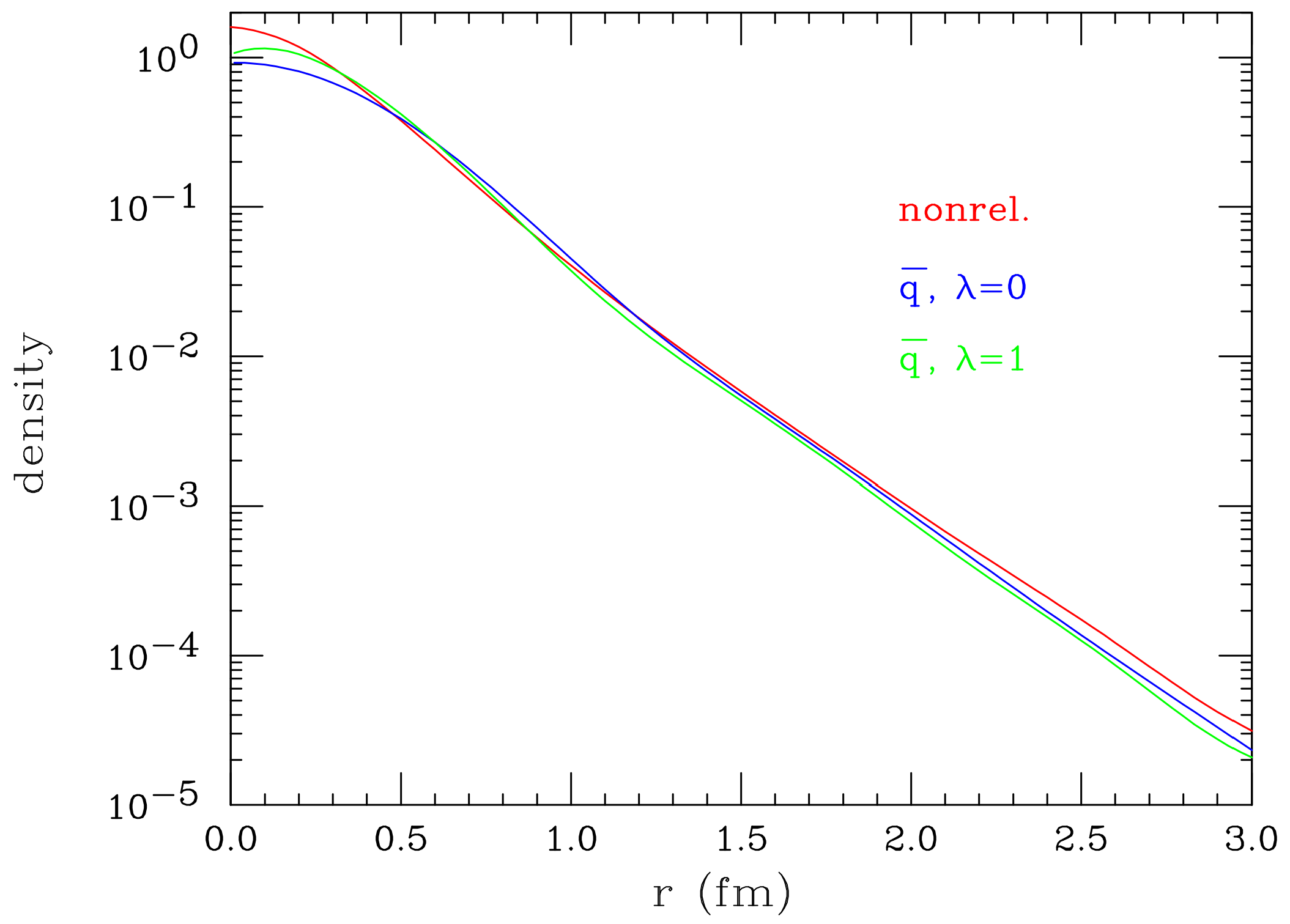
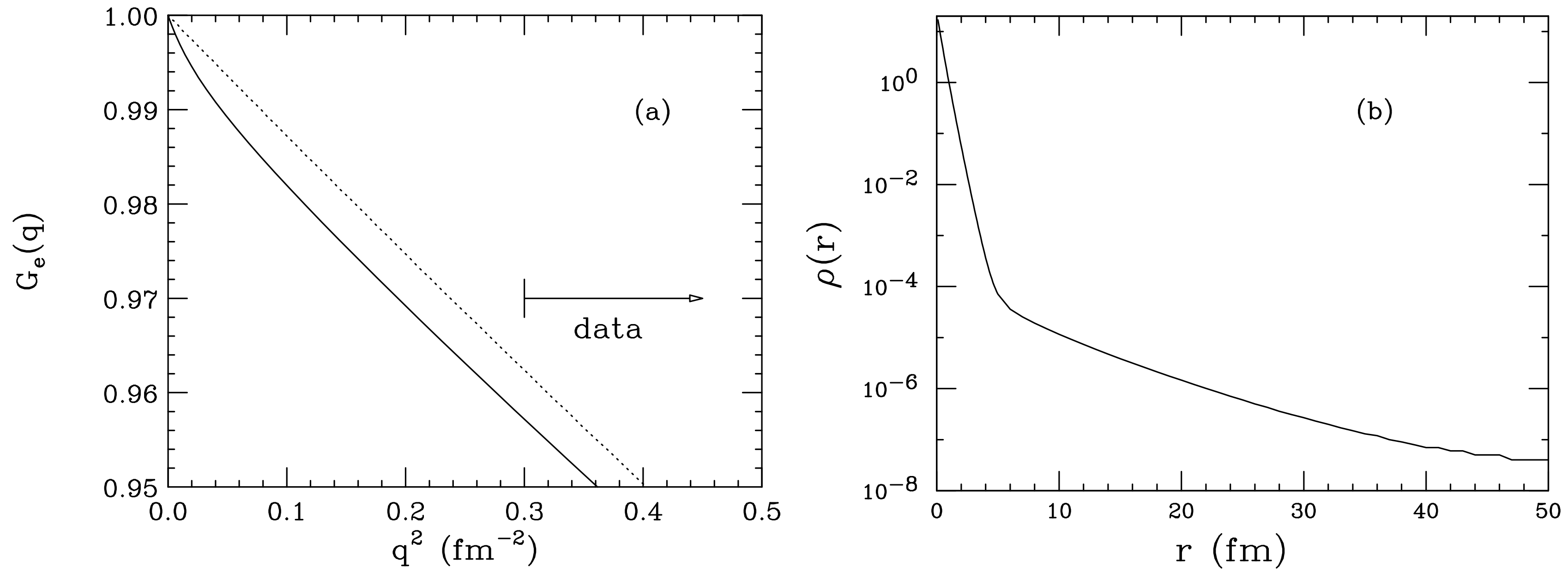
These corrections can be incorporated if a quantitative density is desired. In Figure 1, we show the charge density derived from a parameterized $G_e(q)$ fit to the world data [20], before and after the replacement of q by $\tilde{q}$ and use of the multiplicative factor. The main change occurs for small r, where the density is appreciably reduced. This reduction has a desirable effect: while densities calculated non-relativistically from typical form factors often lead to a kink at $r=0$ (the dipole form factor with the corresponding exponential density is the prime example), the density determined after relativistic corrections is close to flat, as it must be. At $r>1$ fm, the shape of the density is hardly changed, and the relative r-dependence in the range 1–3 fm is changed by a factor of 1.17 only.

Figure 1 shows that the relativistic corrections do not qualitatively change the density one extracts from $G_e(q)$ and that the changes of the r-dependence in the region of large r (particularly relevant for the determination of R; see the discussion below) are small. Despite relativistic corrections, the density remains a valuable quantity to address the properties of the proton and the value of R. We will see below that many of the problems occurring when determining R are much better understood (and largely avoided) when considering $\rho (r)$ as well; this turns out to be true even without using explicit constraints on $\rho (r)$.

The wish to bypass the above relativistic corrections is the reason why the proton rms-radius in the literature is normally hoped to be accessible via the slope of $G_e(q)$ at $q=0$:

$$\begin{array}{c}\hfill R^2=-6\frac{d{G}_e(q^2)}{d{q}^2}{|}_{q=0}\end{array}$$

(6)

without ever considering the underlying density. Restricting the attention to this $q=0$ property has caused many problems in the determination of a precise value for R. The crux lies in the model dependence of the function needed to extrapolate from the q-region where data are available and sensitive to R to $q=0$.

4. Data

Cross-sections for electron-proton scattering have been measured over the past 50 years, and an extensive set of data is available [21,22,23,24,25,26,27,28,29,30,31,32,33,34,35,36,37,38,39,40,41,42,43,44,45,46,47,48,49,50,51,52,53,54,55,56,57,58,59,60,61]. The cross-sections have been measured using gaseous or liquid hydrogen targets and electron beams with energies between ∼50 MeV and ∼20 GeV. The range of scattering angles extends from 8${}^{\circ }$–180${}^{\circ }$. The need to achieve small systematic uncertainties requires accurate measurements of beam intensity (accumulated charge), target thickness, spectrometer acceptance and detector efficiency. The most accurate experiments have been performed at low momentum transfer, where overall systematic uncertainties of order 1% have been reached.

The overall normalization of the cross-sections often is responsible for the dominant systematic uncertainty. As a consequence, many authors who analyze the data consider this overall normalization as a free parameter. Floating the data leads to a significantly lower ${\chi }^2$ for the entire world dataset, but to larger uncertainties of the values of the form factors and derived quantities. A safer alternative may be to keep the normalizations at the measured values, and live with the larger ${\chi }^2$. In this case, the effect of the systematic errors can be determined by changing in turn each set by the quoted systematic errors, refitting the data and adding quadratically all the resulting changes.

The cross-sections are reasonably consistent; when floating the normalizations, the pre-2010 world data (some 604 data points for $q_{max}<10$ fm${}^{-1}$) can be fit with a ${\chi }^2$ per degree of freedom that is close to one. We omit the set of [62], which shows oscillations and yields a much too large ${\chi }^2$.

A recent experiment [39] has tried to achieve significantly smaller error bars by monitoring the product of charge times target thickness with a second spectrometer placed at a fixed angle. This experiment has produced some 1420 cross-sections for $q<5$ fm${}^{-1}$, with error bars of about 0.3%. This approach came at the expense of introducing, for the 34 individual datasets 31 free normalization factors.

The data from this experiment show significant deviations from the pre-2010 data (see Figure 2 of [39]). The reasons for the discrepancy are not entirely understood. One obvious problem of the data of [39] is due to the fact that the contribution of the target windows (5–15%) was not measured, but simulated. This simulation included the radiative tail of the window material, but did not include inelastic scattering from the window nuclei. According to the one measured spectrum shown [63], deviations of the measurements of >1% must be expected.

This discrepancy between the pre-2010 and the Bernauer et al. data complicates the analysis of the world data. It leads to the fact that the authors analyzing the data use one or the other set. The combination (see, e.g., [64,65]) would require an increase of the error bars of [39] by an amount that is difficult to gauge. Use of the data [39] alone is disadvantageous because this set does not provide (due to limitations in beam energy) data at low q and a large angle, resulting in rather limited information on the magnetic form factor and radius.

Despite these difficulties, various analyses [64,65] have shown that for the charge rms-radius, the topic of main interest here, the pre-2010 world and the Bernauer data basically agree.

The quantities measured in an electron scattering experiment do not directly yield the cross-sections. The measurements have to be corrected for the effects of Bremsstrahlung (see, e.g., [66,67]). The corresponding theoretical corrections amount to typically 30% and are believed to not contribute too much to the final overall uncertainty of ∼1%.

During the last two decades, polarized electron beams have become standard at many electron beam facilities. The polarization transfer to the recoiling proton can be measured by placing a polarimeter in the focal plane of the spectrometer used for the detection of the recoil proton. The measurement of the two polarization components provides a very valuable additional observable, which helps to separate $G_e$ and $G_m$. For the polarization transfer data [68,69,70,71,72,73,74,75,76,77,78,79], the overall normalization is less of an issue, as the observable of interest is a ratio of two polarizations.

5. Peculiarities and Difficulties

5.1. Importance of $\rho (r)$ at Large r

From Equation (4), it follows that the charge at radius $r_0$ generates a Fourier component in $G_e(q)$ of type $sin(q{r}_0)/(q{r}_0)$; for large $r_0$, it produces a curvature of $G_e(q)$ at low $q_0\sim \pi /(2r_o)$. The curvature of $G(q^2)$—the deviation from linearity in $q^2$—affects R when the radius is determined via extrapolation from q > $q_{min}$, where data are available and sensitive to R to $q=0$.

The charge density of the proton has a shape that is very different from the typical Woods–Saxon type shapes encountered for heavier nuclei. The proton form factor is roughly described by the dipole shape:

$$\begin{array}{c}\hfill G_D(q)=1/{(1+q^2{R}_D^2/12)}^2.\end{array}$$

(7)

The density corresponding to this form factor has the shape of an exponential:

$$\begin{array}{c}\hfill {\rho }_D(r)\propto e^{-\sqrt{12}r/R_D}.\end{array}$$

(8)

Such a density exhibits a long tail towards large radii, which contributes appreciably to the rms-radius.

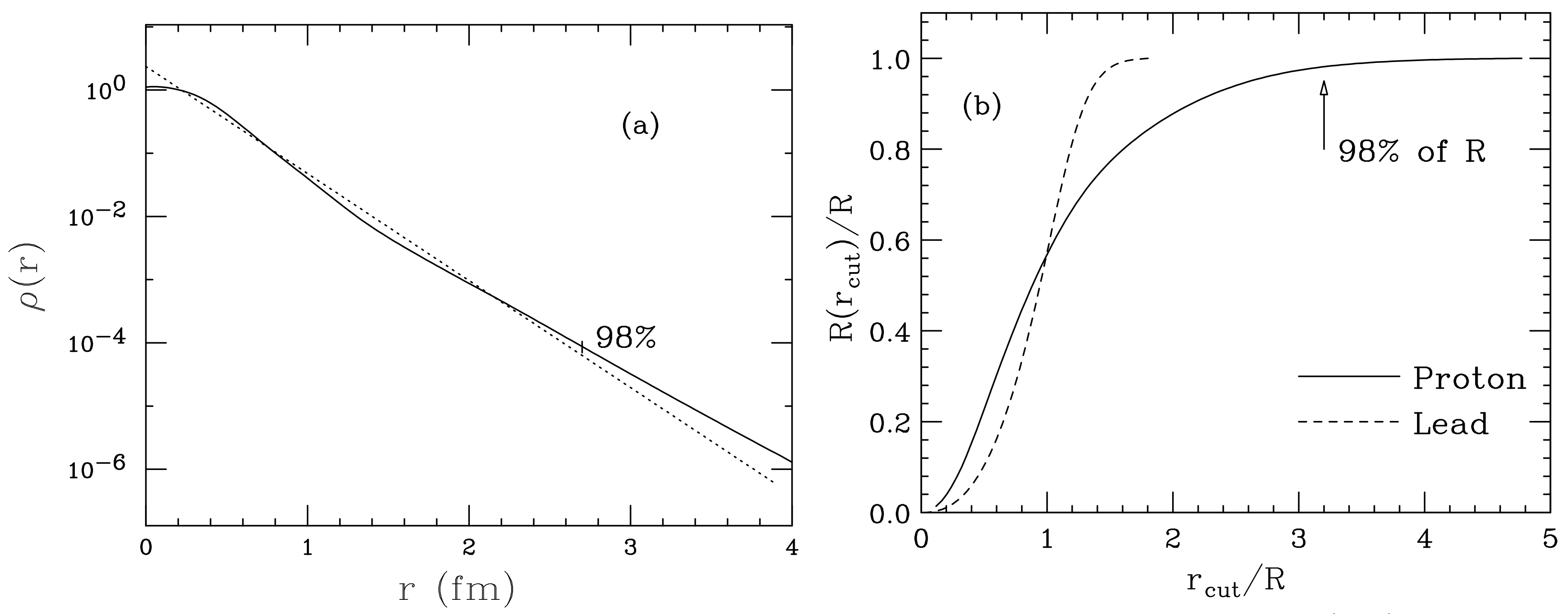
In Figure 2a, we show the density corresponding to a dipole form factor (dotted) and a more realistic one (solid) resulting from the fit to the electron scattering data. In Figure 2b, we show the partial integral:

$$\begin{array}{c}\hfill R\left(r_{cut}\right)={\left[{\int }_0^{r_{cut}}\rho (r)r^{4}dr/{\int }_0^{\infty }\rho (r)r^{4}dr\right]}^{1/2},\end{array}$$

(9)

with the rms-radius given by $R=R(r_{cut}=\infty )$. To get 98% of R, one has to integrate out to 2.7 fm, where the density has dropped to ∼10${}^{-4}$ of the central value!

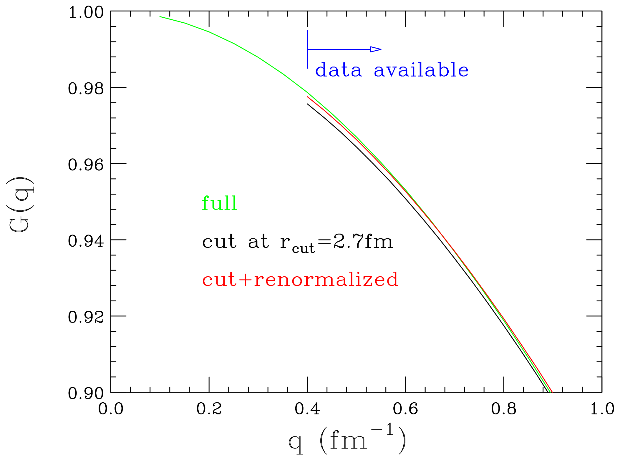
The effect of $\rho (r>2.7$ fm) on $G_e(q)$ at low q is explored in Figure 3 where we show the form factor $G_e(q)$ for three cases:

• Dipole form factor (exponential density).
• Form factor corresponding to exponential density truncated at $r_{cut}=2.7$ fm.
• Form factor corresponding to truncated density, renormalized to agree best with the Dipole form factor for momentum transfers above the minimum momentum transfer of the data; this renormalization corresponds to the standard renormalizations of data applied in most analyses.

The difference between Case 1 and 3 is less than 0.12% of $G(q)$, which is much smaller than the uncertainties most experimentalists would claim to be able to achieve. Due to the renormalization, one would miss the curvature of $G_e(q)$ and the contribution to R from the larger-r density, which for the example chosen, amounts to 2%. The same argument could be extended to a cut at 2.4 fm, yielding a 4% deviation of R. We will come back to this point below. This problem can only be solved by constraints on the model-$G(q)$ based on the physics of the density at large r, but not by curve-fitting of data of realistic precision in the low-q region.

5.2. Smallness of Contribution of R to $G_e(q)$

When analyzing data with parameterized expressions for $\rho (r)$ or $G_e(q)$, one needs to be aware of the potential size and location in q of the main contribution of R to $G_e(q)$. To this end, it is helpful to consider a so-called notch test.

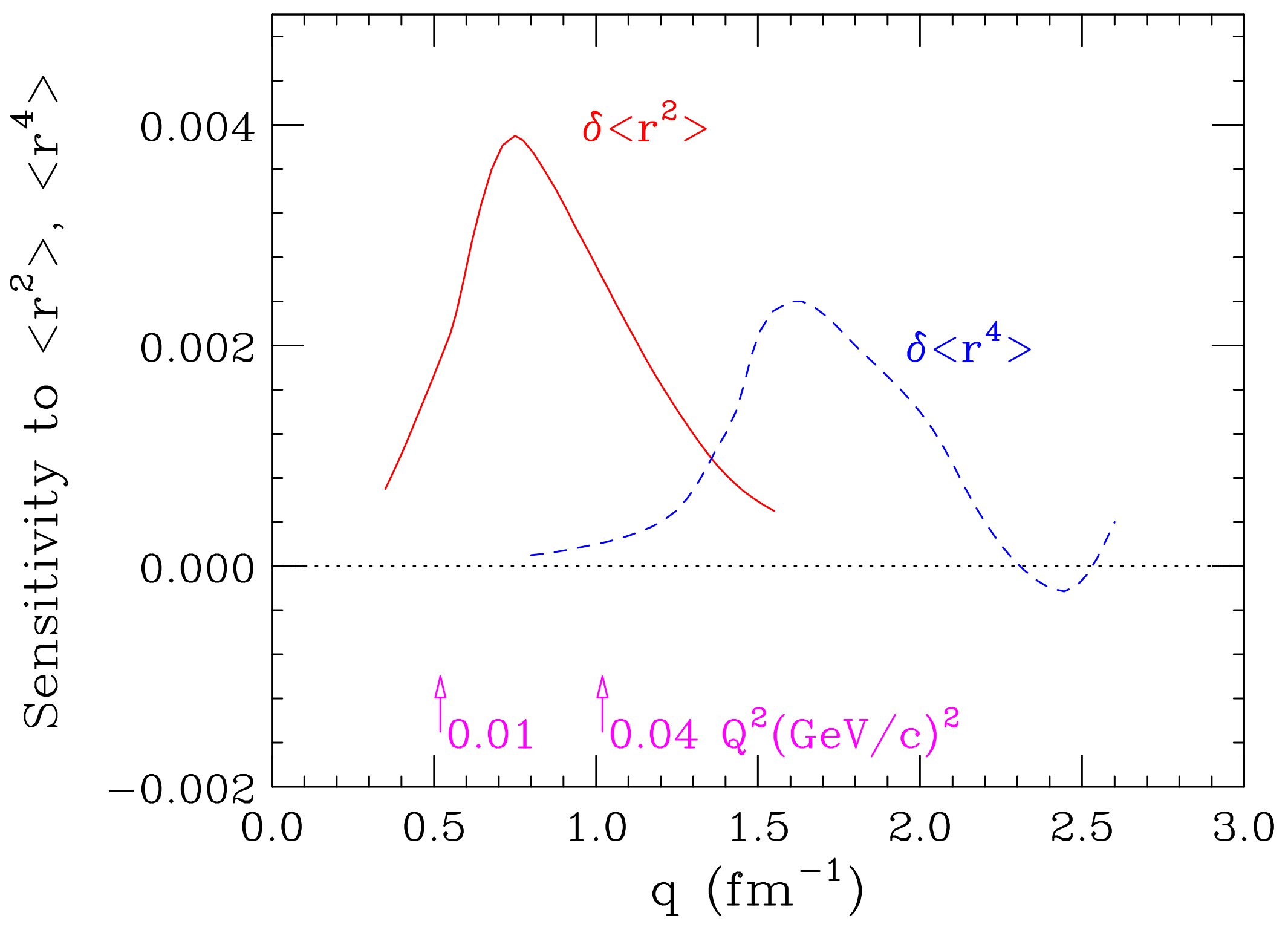
This test is carried out as follows: the world data are fit with a flexible parameterization for both charge and magnetization densities, yielding rms-radii R together with the higher moments of interest. The data in the interval of $\pm 0.1$ fm${}^{-1}$ around $q_n$ then are increased by 1%. The modified data are fit, resulting in a change of the rms-radii (and eventual higher moments). This procedure is repeated for varying $q_n$, and the resulting changes of the radii (and higher moments) are plotted as a function of $q_n$. Figure 4 shows typical results.

Figure 4 displays the expected behavior: at very low q, the form factor is not sensitive to R because of the smallness of the contribution of R to $G_e(q)\sim 1-q^2{R}^2/6+\dots$; at the larger q’s, the effects of the forth (and higher) moments dominate. The world data in the q-region $0.5÷1.2$ fm${}^{-1}$ thus are mainly determining R. The region of sensitivity for the Zemach radii [80,81] is quite similar.

At the momentum transfer of maximal sensitivity to R, $q\sim 0.8$ fm${}^{-1}$, the contribution of R to $G_e(q)$ amounts to $q^2{R}^2/6\sim 0.08$. A determination of R to 1% then would require knowledge of $G_e(q)$ to ±0.0016, i.e., ±0.17%. This emphasizes that a fit of the e-p data aiming at a 1% determination of R must achieve systematic deviations from the experimental $G_e(q)$ that are smaller than 0.17%. This can only be achieved by fits that reach the smallest ${\chi }^2$ possible (and in any case, smaller than achieved by other fits). Fits that visually look good (for examples, see [82,83,84,85]) are no proof of small systematic deviations from the data, simply because the plots of data vs. fit shown in many papers published in the past do not by far have the resolution that would allow one to detect a systematic deviation of order 0.17%. Fits that achieve low ${\chi }^2$ by rescaling the error bars of the data, as done in, e.g., [84], are not valid; fits to exactly the same data with a ${\chi }^2$ lower by ∼300 are available.

5.3. Parameterizations in q-Space Only?

Due to the complications mentioned in Section 3, most authors analyzing the electron scattering data employ parameterizations in q-space only to get the $q=0$ slope, without ever worrying what these parameterizations would imply in r-space. This omission often leads to uncontrolled effects; in the following, we discuss examples to illustrate this point.

We have some time ago [86] analyzed the data of [63] for $q<2$ fm${}^{-1}$ using a parameterized $G(q)$. Data for $q_{max}=2$ fm${}^{-1}$ are usually considered sufficient for a precise determination of R; see Figure 4. The parameterization employed was a [1/3] Padé approximant:

$$\begin{array}{c}\hfill G(q)=\left[1+a_1{q}^2\right]/\left[1+b_1{q}^2+b_2{q}^4+b_3{q}^6\right].\end{array}$$

(10)

With this function, the data can be fit with a ${\chi }^2$, which is as low as the ${\chi }^2$ obtained for the same data in [63] with a spline fit. The Padé function has none of the failures occasionally encountered in the literature—poles or unphysical behavior for $q\to \infty$—but it produces a charge rms-radius R of 1.48 fm! Figure 5a shows the behavior of $G_e(q)$ at very low q, below the range covered by the data. The Padé fit exhibits a curvature at $q^2<0.05$ fm${}^{-2}$, leading to the large slope at $q=0$ and correspondingly large R. This fit is compared to a “standard” fit corresponding to $R\sim 0.88$ fm (dotted). Both fits explain the data perfectly (not shown); for $q^2>0.2$ fm${}^{-2}$, the fits differ by an overall normalization of ∼1% in $d\sigma /d\Omega$, but give the same ${\chi }^2$, as the normalization of the data is floating.

This educational example demonstrates that it is important to examine the density implied by the parameterized $G(q)$. In r-space, the outrageous behavior of the Padé fit is immediately visible (see Figure 5b), and it occurs despite the fact that the formal expression for the [1/3] Padé parameterization (Equation (10)) looks as acceptable as other q-space parameterizations employed in the literature. The peculiar nature of the fit results from the correlation between $a_1$ and $b_1$, which, when assuming large values, can generate the behavior shown in Figure 5.

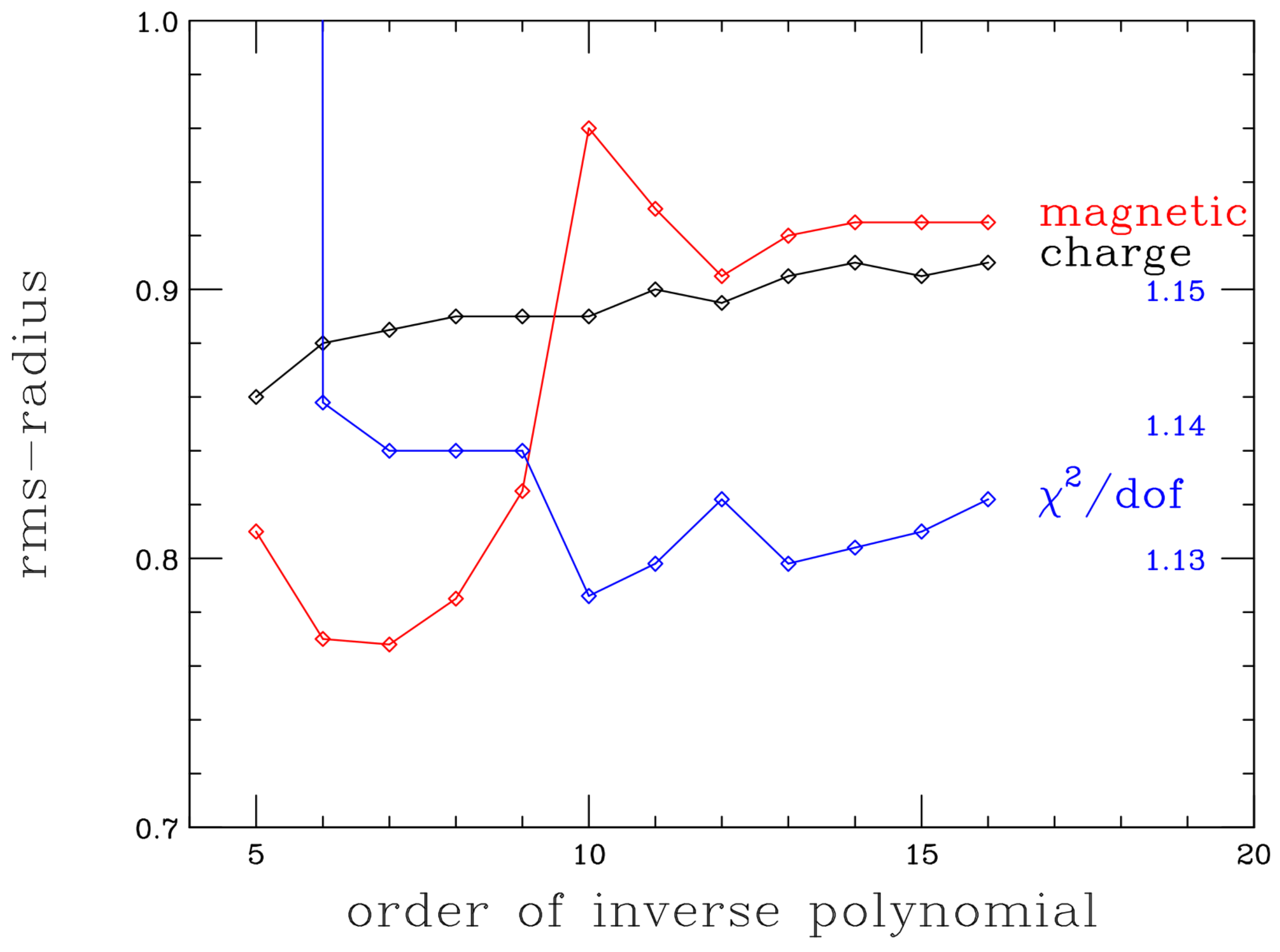
There are other examples in the literature that emphasize the importance of considering $\rho (r)$ at the same time. Bernauer et al. [63], for instance, make an inverse polynomial fit to their data ($q_{max}\sim 5$ fm${}^{-1}$). The resulting values for R as a function of the order of the polynomial are plotted in Figure 6. The jump of $R_m$ at order 10 (not used for the determination of R) results from a pole of $G(q)$, which happens to occur close to the $q_{max}$ of the data. Such a form factor with a pole corresponds to a density that shows large-amplitude oscillations out to very large values of r [87], which of course affect R. A look at the density would have immediately revealed the unphysical nature of the form factor fit.

The lesson from the above examples is that it is important to check on the behavior of the density implied by the chosen $G(q)$. The most important corollary is that it is very dangerous to employ parameterizations that do not even correspond to a physical density, such as the large majority of published parameterizations that are not consistent with a large-q fall-off, which is at least as steep as $q^{-4}$. Since the data alone are not sufficiently accurate to fix the low-q curvature, this quantity then (in the absence of physics constraints on the large-r $\rho (r)$) is mainly given by the choice of the model for $G(q)$ used for the extrapolation; aberrant results for R such as illustrated by the above examples then cannot be identified and excluded. One basic problem: the parametrization can contain $sin(qr)/qr$-components (see Equation (3)), which imply contributions from unphysically large radii of, say, $r>3$ fm.

5.4. R from Very-Low-q Data?

Starting from the idea that R can be determined from the $q=0$ slope of $G(q^2)$, the form factor is often parameterized as a power series in $q^2$, $G(q^2)=1-q^2{R}^2/6$ plus eventual higher terms in $q^2$ (see the discussion below). With precise data at low enough $q^2$, one could hope to determine the $q^2{R}^2/6$ term to, say, %-type accuracy without worrying about the higher-order terms in $q^2$.

The problem with this approach is two-fold:

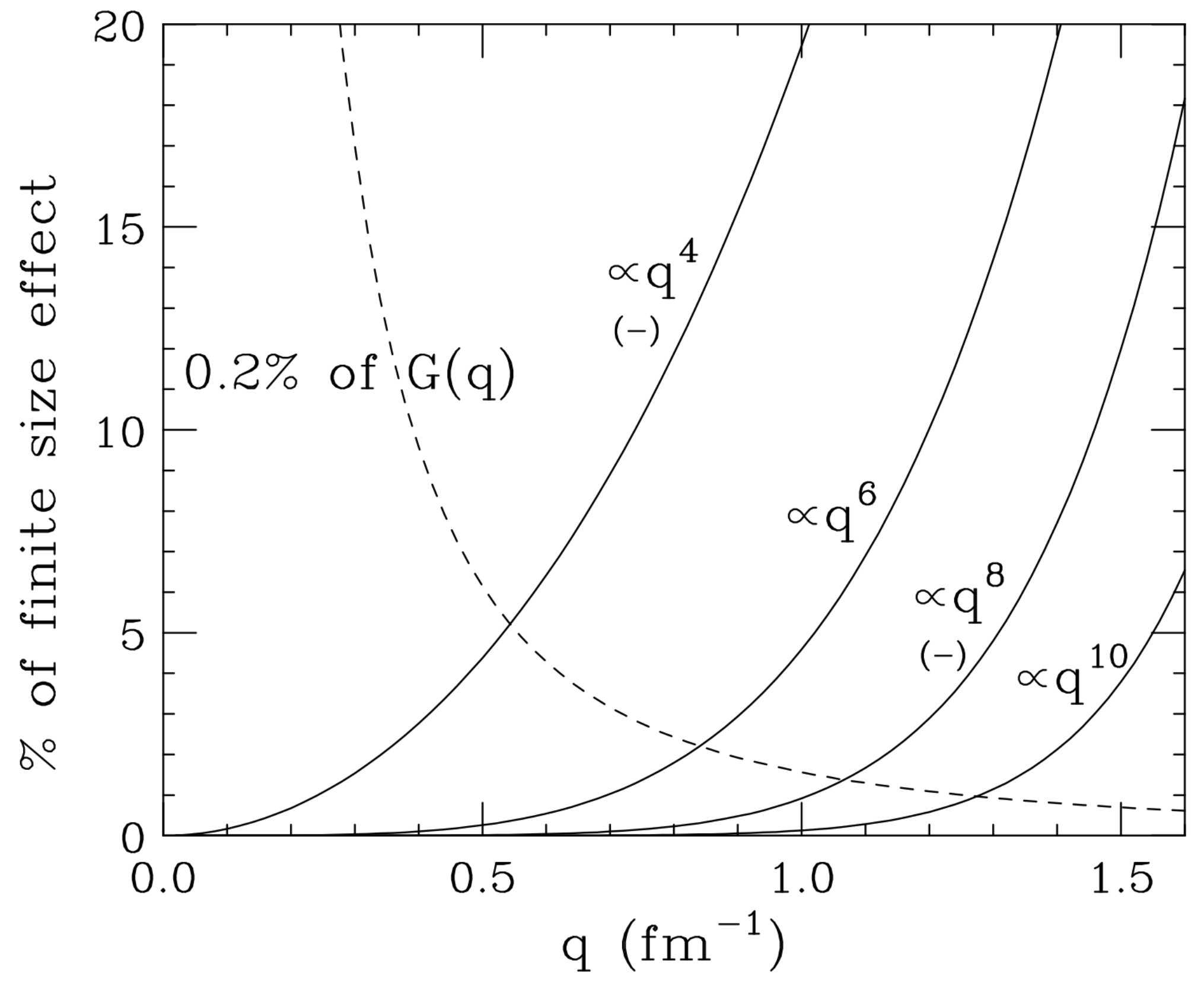
• Due to the peculiar shape of the proton density, the moments $\langle r^{2n}\rangle$ are large and the $q^{2n}$-terms strongly coupled [15]. This is illustrated in Figure 7 [88], which shows the contributions (in %) of the higher moments to the finite size effect FSE $1-G(q)$. In order to make the contribution of $n\ge 2$ smaller than, say, 1% in R (2% in FSE), one has to restrict $q_{max}$ to an extremely small value of ≤0.34 fm${}^{-1}$ (0.004 GeV${}^2/c^2$).
• At these low q’s, the term of interest $q^2{R}^2/6$ becomes very small—0.015 at $q\sim 0.34$ fm${}^{-1}$—but the experimental uncertainty of the measured quantity $G\sim 1$ remains of order 0.01. A measurement of $R^2$ to, say, 2% (1% in R) then would require a measurement of G to 0.015·2% = 0.03%. Such an accuracy is not within reach for a very long time. Extracting an accurate $q^2=0$ slope directly from a measurement [89] without dealing with the higher moments (without extrapolations) is pretty hopeless.

5.5. A Counter-Intuitive Observation

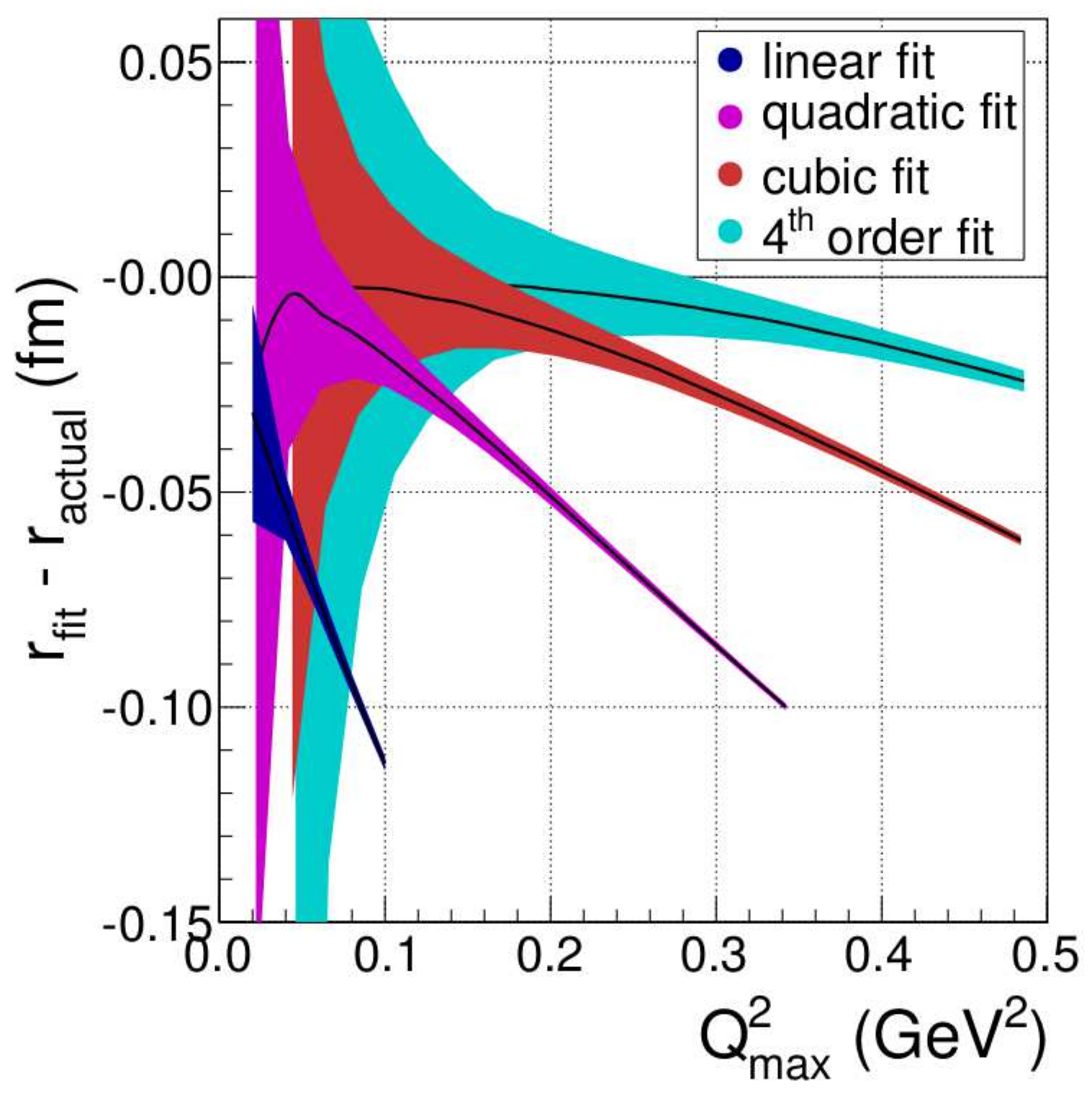
In several of the published analyses of e-p data, the dependence of the extracted radius R on the maximum momentum transfer $q_{max}$ of the data employed has been studied. These works have often produced an apparently counter-intuitive result: the value of R changes significantly with $q_{max}$. As an example, we show in Figure 8 the results of Lee et al. [64].

This dependence of R on $q_{max}$ at first sight seems incompatible with the idea that R is obtained from the slope of $G_e(q)$ at $q=0$. Why do the high-q data have such an impact? It can be understood once one realizes that the basic difficulty of the determination of the $q=0$ slope rests on the extrapolation from q’s, where the form factor is sensitive to R (see Figure 4) to $q=0$. The extracted $q=0$ slope depends on the curvature of the parameterization at the q’s below ∼0.6 fm${}^{-1}$. The more we know about the density, the better we can constrain this curvature of the extrapolating function. In particular, knowing more about the shape of the density including its large-r tail fixes better the shape of the form factor at low q, as explained in Section 5.1. In order to fix best the shape of the density, the density should explain the full set of $G_e(q)$ data. It can easily be made plausible that fixing the density including the large-r tail region requires fitting the data up to the largest momentum transfers.

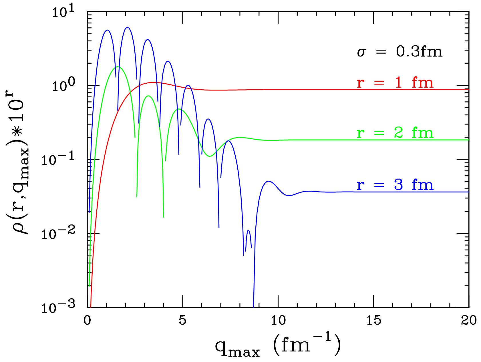
We illustrate this point with a pedagogical example. Consider the density as the truncated Fourier transform of $G_e(q)$, defined as:

$$\begin{array}{c}\hfill \rho (r,q_{max})=\frac{1}{2{\pi }^{2}r}{\int }_0^{q_{max}}{G}_e(q)sin(qr)qdq,\end{array}$$

(11)

with $\rho (r)=\rho (r,\infty )$. In Figure 9, we show $\rho (r,q_{max})$ calculated for three values of r using the standard dipole form factor, Equation (7). To reduce the oscillations resulting from the sharp cut-off of the integral at $q_{max}$, the $\rho (r,q_{max})$ is averaged over a region around the selected r with a Gaussian weight of width $\sigma$, such that the values plotted represent some average density in the region centered at r; obviously, it is only this average density that is relevant for the shape of $G_e(q)$ at low q.

Figure 9 shows that for $r=1$ fm, the (averaged) density is well determined once the upper limit of the integral has reached about 5 fm${}^{-1}$. For larger r, higher $q_{max}$ is needed; the density in the $r=3$ fm region is only reasonably determined once $q_{max}\sim 11$ fm${}^{-1}$. Due to the smallness of $G(q)$ at large q, the high-q data help to determine the small-amplitude Fourier components, which are important to fix the small densities occurring at large r. Figure 9 shows why fits that explain the data up to larger $q_{max}$ fix better the density at larger r, hence yielding (implicitly) a more realistic shape of the $G_e(q)$ needed to extrapolate to $q=0$. We therefore in this review concentrate on the pre-2010 data, which reach the higher $q_{max}$.

To summarize: the extrapolation of low-q data to $q=0$ is most often based on model-dependent parameterization of $G(q)$. Much more reliably, the shape of $G(q)$ can be constrained by the shape of $\rho (r)$ at large r known (implicitly) from fits to data up to the highest q’s, and these fits produce the most trustworthy values of R. As will be shown in Section 6.3, Section 6.4 and Section 6.5 fits including the large-q data yield large-r tails of $\rho (r)$ that are “well-behaved”, i.e., are close to the one obtained with a physics constraint as described in Section 6.8, Section 6.9 and Section 6.10.

6. Parameterizations and Fits

The data on electron-proton scattering have been analyzed in the past by a number of authors. Different procedures have been employed, and a variety of parameterizations have been used. Below, we discuss a representative set, from which in the end we aim to distill a reliable value for the rms-radius.

6.1. Types of Parameterizations Used

• For the interpretation of data at very low values of q, various traditional expressions, depending on one or two parameters, have been used: dipole, double dipole, Gaussian, Yukawa, etc.; see, e.g., [82,90]. Only those parameterizations are retained that give a ${\chi }^2$ close to the minimal one found. The obvious risk of this approach is that parametrizations with too few degrees of freedom yield too large ${\chi }^2$ and unreliable R [82,83,84]. Figure 7 can be used to estimate how many independent parameters (moments) are needed to achieve a given accuracy of R for a given $q_{max}$.
• When fitting data up to large q, which requires many free parameters, a different approach is needed. Multi-parameter models such as the Padé form factors [15,91], polynomials or inverse polynomials of high order [90,91,92] or polynomials as a function of derived quantities [64,93,94] have been employed. Typically, the number of parameters is increased until the ${\chi }^2$ per degree of freedom reaches a plateau. Occasionally, the model dependence is estimated by generating and fitting pseudo-data and comparing the fit-results to the known input values [15,90,92,94].
• A somewhat more systematic approach employs an expansion of the form factors on an orthogonal basis [19,95,96]. This eases the determination of the parameters, but the selection of the appropriate cut-off in the order of the expansion (mostly based on the ${\chi }^2$-plateau argument) is more delicate. The use of Gaussian bounds on the individual parameters, implemented by a “penalty” contribution to ${\chi }^2$ [64,93,97], is also quite efficient in limiting the values of the highest-order coefficients, which tend to be poorly constrained by the data.
• Safer approaches try to include known physics in the parameterization, hereby restricting the freedom of the fit. Examples are the Sum-Of-Gaussians (SOG) densities, which limit the fine structure in the density [98], or semi-phenomenological Vector Dominance Model (VDM)-based fits, which employ the analytical form of the VDM-$G(q)$ and/or constrain the large-r fall-off; see [99,100,101,102,103] and Section 6.8 and Section 6.9.
• The strongest (and often too strong) input from theory is present in approaches such as the VDM fits, where constraints come from the assumption of vector dominance and the experimentally-known masses and couplings of the vector mesons (see Section 6.7).

6.2. Polynomials in q

Given that the rms-radius most often is thought of as the slope of the form factor at $q=0$, it is popular to employ for the parameterization of the Sachs form factors $G_e$ and $G_m$:

$$\begin{array}{c}\hfill G(q)=1+a_2{q}^2+a_4{q}^4+a_6{q}^6+\dots ,\end{array}$$

(12)

with $a_2$ = $-R^2$/6 and, non-relativistically, $a_4=\langle r^4\rangle /120$ and $a_6$ = $-\langle r^6\rangle /5040$ given by the higher moments of the density distribution.

The above expression is often taken as the Taylor expansion of $G(q)$ around $q=0$, in which case the question of the convergence radius ($q^2$ = 4$m_{\pi }^2$ in the VDM) can come up. Alternatively, one can take this parameterization simply as a polynomial fit in the selected q-range, in which case the parameterization is not subject to this concern. For a discussion, see [104].

We have pointed out a long time ago [15] that a polynomial fit is not suitable; the rms-radius and higher moments are very dependent on the cut-off $q_{max}$ and the number of terms employed. This is essentially a consequence of the fact that for an exponential-type density, the higher moments increase rapidly with order. As a result, the convergence of $G(q)$ with order is poor: the contributions of the higher terms grow and are alternating in sign (see also Figure 7).

Kraus et al. [92] have demonstrated the inadequacy of the polynomial fits in a quantitative manner. They generated pseudo-data, in a realistic q-range with realistic error bars, using different parameterized form factors with known $R_{actual}$. These data were fit using the above polynomial expression and the resulting $R_{fit}$ compared to $R_{actual}$. Their result is shown in Figure 10 as a function of the upper limit $q_{max}$ and for different orders of the polynomial. For a cutoff at low $q_{max}$, the error bars on R (shaded areas) are large; for higher cutoffs the error bars get smaller, but the resulting values of $R_{fit}$ are systematically below the input value. Polynomial fits simply give wrong results, such as the radii of [83,84] in the 0.84 fm region; see [88].

The behavior shown in Figure 10 can be understood qualitatively. Consider, e.g., a linear fit of the very-low q data with $G_e(q)$ = 1 $-q^2{R}^2/6$ [83,84], with all higher moments set (implicitly) to zero. The most important neglect then is due to the lowest higher moment $\langle r^4\rangle$. A charge distribution with $\langle r^2\rangle$ finite and $\langle r^4\rangle$ = 0 must have a pronounced negative tail at large r, needed to reduce $\langle r^4\rangle$ to zero. This negative tail of course also affects $R^2$ and leads to the behavior exemplified by Figure 10 (dark blue curve). The same thing happens if the parameterization is cut off at higher order.

The above reasoning on the charge density is, of course, only a plausibility consideration. In reality, there is no physical charge distribution that could correspond to a polynomial-type form factor, since the Fourier transform of any polynomial expression diverges.

Polynomials in q or $z(q)$ (see Section 6.4) have another generic (and serious) problem. The functional dependence does not naturally embody the fact that form factors are steeply falling with increasing q. As a consequence, the small values of $G(q)$ at large q have to be generated by delicate cancellations including the low-order terms, which typically give the largest contribution to FSE near $q_{max}$. For, e.g., the parameterization of Lee et al. [64] (to be discussed below), the term $a_{1}z$, which is meant to parameterize the $q^2=0$ slope and determine R, still contributes 70% of the finite size effect FSE = 1$-G_e(q)$ at the maximum q of 5 fm${}^{-1}$ employed, leading to undesirable correlations affecting R. For polynomials in $q^2$, this disease is even worse (400% of FSE at 5 fm${}^{-1}$).

6.3. Inverse-Polynomial Type

The standard polynomial-type parameterization discussed above has a number of properties that make it unsuitable. An inverse polynomial, such as used for instance by Bernauer et al. [90], avoids the problem of divergence in the $q\to \infty$ limit. However, it retains the undesirable feature of strong correlations between the individual terms, leading to coefficients with alternating signs that grow with order. Zero’s of the polynomial, leading to poles in $G(q)$ (in general at $q>q_{max}$) addressed already in Section 5.3 and the steep fall-off of inverse-polynomial $G(q>q_{max})$ then lead to densities that show oscillations out to unphysically large radii.

A variant is the Padé parameterization, which often is the “best” approximation of a curve by a rational function of given order:

$$\begin{array}{c}\hfill G(q)=\left(1+\sum _{i=1}^I{a}_i{q}^{2i}\right)/\left(1+\sum _{j=1}^J{b}_j{q}^{2j}\right).\end{array}$$

(13)

If the coefficients in the denominator are constrained to $b_j>0$ and the order J to $J\ge I+2$, poles and divergences are avoided. This function has been used by Kelly [20] and Arrington et al. [91]. The latter authors have performed a fit to the pre-2010 world data ($q_{max}=10$ fm${}^{-1}$) including two-photon corrections. Their fit (not especially oriented towards a determination of R) has an excellent ${\chi }^2$ and yields $R=0.878$ fm. The corresponding density (see Figure 1) is “well behaved”, i.e., falls at large r similarly to tail densities obtained with physics constraints (to be discussed with Figure 12).

Special cases of the Padé parameterization, in the form of Continued Fraction (CF) expansions, have been employed in [15,83,84,105]. Besides the difficulties mentioned above, finding the parameters of the global best-fit was sometimes not successful [104]. CF fits with too few parameters [84,105] yield values of ${\chi }^2$ that are much larger than other published fits to the same data, hence yielding no reliable R.

6.4. Polynomials in z(q)

Dispersion relations show that the form factor is an analytic function of t = $-q^2$, with a cut beginning at the two-pion threshold $q_{cut}^2$ = $-t_{cut}$ = $-4m_{\pi }^2$. Hill and Paz [93] exploit this by mapping q onto the variable:

$$\begin{array}{c}\hfill z(q^2)=\left(\sqrt{t_{cut}-t}-\sqrt{t_{cut}-t_0}\right)/\left(\sqrt{t_{cut}-t}+\sqrt{t_{cut}-t_0}\right),\end{array}$$

(14)

with $t_0$ usually set to zero. At small momentum transfer, z is proportional to q, while at large momentum transfer, $z\to 1$. Paz and Hill then expand the form factor as a power series in z, $G(z)=\sum a_k{z}^k$. For the physical region, this implies the existence of a small expansion parameter z < 1.

Use of z maps the cut onto the unit circle in the complex variable z, which is hoped to reduce the curvature in the form factor, which complicates the extrapolation to $q=0$. The curvature of $G(z<z_{min})$ is indeed reduced by ∼30% [93], but this does not really remove the problem of the unknown curvature of the true form factor.

The advantage of the expansion in terms of z is that the coefficients multiplying $z^k$ are bounded. Lee et al. [64], who present an extensive and very detailed analysis of the e-p world data using the same approach, employ a uniform bound on $a_k/a_0$, enforced by an additive penalty $a_k^2/a_0^2$ in the ${\chi }^2$. This has the benefit of making uncritical the number of parameters used, contrary to the standard approaches where too many parameters can lead to an over-fitting of fluctuations of the data and error bars that blow up. For the z-expansion without such bounds [85], the parameters get huge, and no stable solution for R is found (for examples, see [104]).

From a careful analysis with a multitude of fits, Lee et al. deduce a charge rms-radius $R=0.916\pm 0.024$ fm. The authors attribute the larger-than-usual value of the radius to the use of the physics constraint introduced by the z-expansion.

One obvious problem with the polynomial in terms of z is that the form factor in the limit $q\to \infty$ goes to a constant value, of order one. This means that there exists no physical density that corresponds to this $G(q)$. It then is not possible to check whether the curvature of $G(q)$ at q’s below ∼0.6 fm${}^{-1}$ would correspond to a sensible large-r behavior of the density.

In order to investigate the origin of the large rms-radius found by Lee et al., we have repeated their analysis using the same z-variable, but optionally assumed for $G(z)$ a power series in z times a dipole in q. This parameterization is similar to the one proposed by Borisyuk [94]; see below; the polynomial in this case describes only the deviation from the (dominant) dipole q-dependence, while the dipole fixes the generic problem of polynomials discussed at the end of Section 6.2. For this parameterization of $G(q)$, a physical density does exist, and one can check whether the density falls at large r like densities with a tail constrained by physics (to be discussed with Figure 12). When replacing the polynomial in z by this parameterization of $G(z)$, but otherwise following closely the approach of Lee et al., we find a systematic change of the charge rms-radius of ∼$-0.03$ fm and a large-r tail, which is close to the one obtained with a physics constraint as described in Section 6.8, Section 6.9 and Section 6.10.

From this study, we conclude that it is not the mapping into the variable z that is responsible for the large R of [64], but rather some hard-to-identify peculiarity of the unphysical $G(z(q))$.

6.5. Polynomial in $\xi$ Times Dipole

In analogy with the study of Lee et al. discussed above, Borisyuk [94] also maps q into a new variable:

$$\begin{array}{c}\hfill \xi =q^2/(1+q^2/{\xi }_0),\end{array}$$

(15)

with ${\xi }_0$ = 0.71$Ge{V}^2/c^2$. This $\xi$ is very similar to the z-variable of Lee et al., the main difference being that it reaches ∼$0.7$ rather than one in the limit $q\to \infty$. To parameterize $G(q)$, Borisyuk uses:

$$\begin{array}{c}\hfill G(q)={(1-\xi /{\xi }_0)}^2\sum a_k{\xi }^k\end{array}$$

(16)

which, as compared to Lee et al., has an additional factor ${(1-\xi /{\xi }_0)}^2=1/{(1+q^2/{\xi }_0)}^2$ corresponding to the standard dipole. Multiplication with this factor ensures a physical behavior of $G(q)\sim q^{-4}$ in the large-q limit.

Borisyuk determines the optimal parameters by looking, for a given number n of terms, at the error bars of R as a function of $q_{max}$ of the data. For decreasing $q_{max}$, the uncertainty $\delta R$ of R grows due to the statistical errors of the data and the smallness of the Finite Size Effect (FSE); for increasing $q_{max}$, the uncertainty grows due to increasing systematic error resulting from a poor fit of the data; this latter contribution is estimated by comparing R from fits of pseudo-data to the R used to generate the pseudo data. In between, the uncertainty has a minimum, which is taken as $\delta R$. For the combination n = 5, $q_{max}$ = 5 fm${}^{-1}$, Borisyuk finds for R a value of $0.914\pm 0.011$ fm.

In his fits, Borisyuk uses much of the pre-2010 cross-section data, but does not include the polarization transfer data, which are very important to reliably separate $G_e$ and $G_m$. He also does not include some of the older, yet precise, data at very low q.

Repeating his analysis with our pre-2010 cross-section database, the available polarization transfer data and the two-photon corrections of [10], we find, for $q_{max}=5$ fm${}^{-1}$, $R=0.880$ fm. The density for $r>2.4$ fm falls more slowly than the Monopoles times Dipole (MD) density (Figure 12), but approaches it when extending $q_{max}$ to 10 fm${}^{-1}$.

6.6. R from Bayesian Inference

Graczyk and Juszczak [97] present an analysis of the world data that is based on a very different philosophy. In their approach, based on Bayesian inference, the two form factors are assumed to come from a large class of possible models, each described by a functional form depending on a number of parameters. They use neural networks with one hidden layer and a variable number of neurons; as such, a structure is able to approximate any function in principle. The weights of the neural network function are then determined using the Bayesian theorem and as the maximum a posteriori (MAP) for each model. For the likelihood, they used a ${\chi }^2$ distribution. In order to avoid an overfitting of the experimental results, a prior distribution on the parameters, that is the weights of the individual neurons, is added. This is assumed to be of a Gaussian form with the width optimized, as well. Such a prior can be seen as a (Tikhonov) regularization of the result, preferring smooth functions. The comparison of the different models, given by different numbers of neurons and therefore different model complexity, is done by approximating the model evidence with the MAP value of the likelihood together with the Occam factor to take into account the uncertainty of these values.

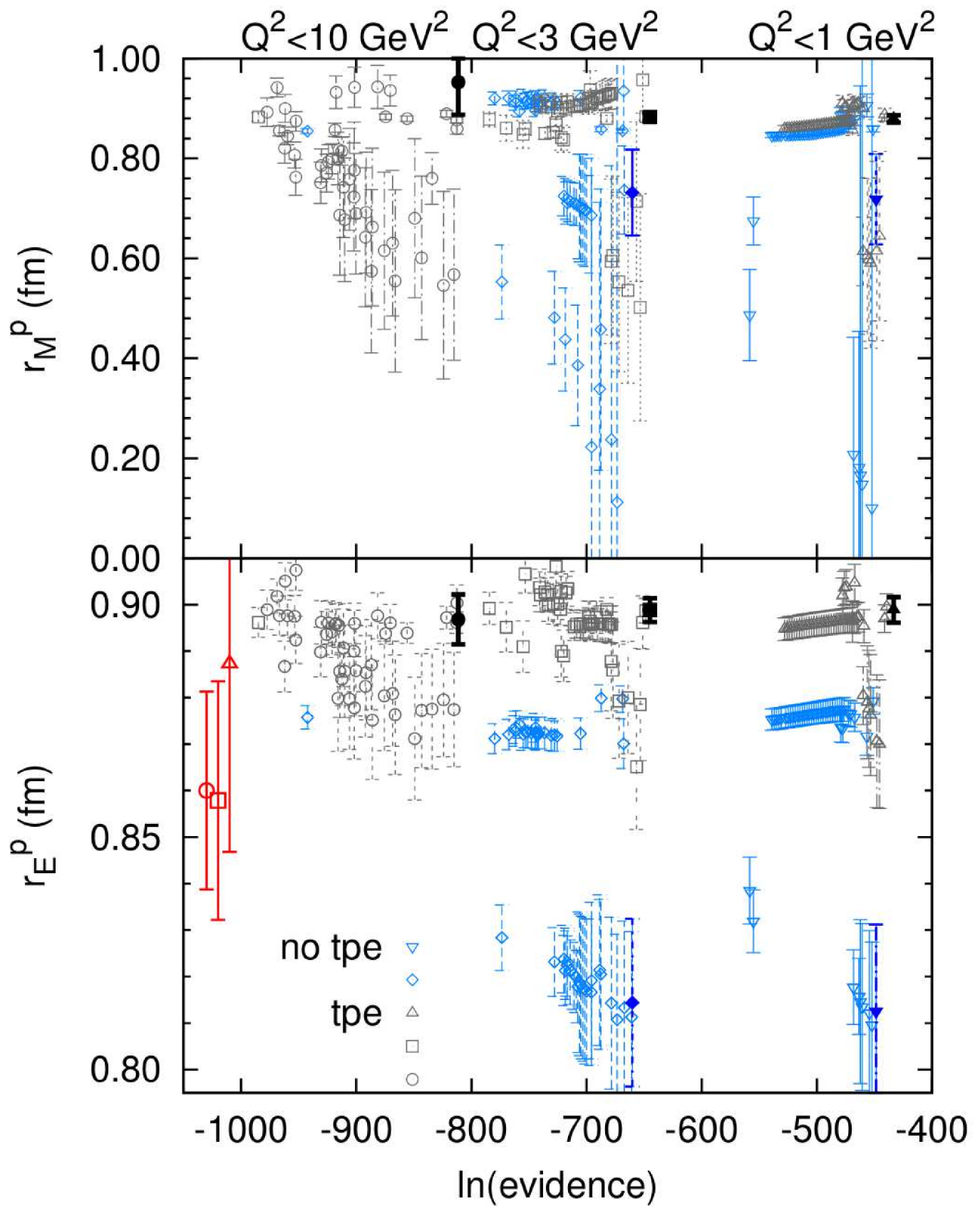
Graczyk and Juszczak have applied this approach to the pre-2010 world cross-section data including the polarization transfer results. The input data were corrected for the effects of two-photon exchange. The resulting radii, for three different values of $q_{max}$, are plotted in Figure 11 as a function of the evidence. The density, calculated from the coefficients given in [106] ($q_{max}\sim$ 10 fm${}^{-1}$), is well behaved and out to 2.7 fm very close to the MD and SOG densities (to be shown in Figure 12), which include a physics constraint at large r. From these values, the authors extract the charge-rms radius, which for the three values of $q_{max}$ of Figure 11, amounts to 0.899(0.003), 0.899(0.003) and 0.897(0.005) fm, respectively. The error bars appear low given the size of the systematic (normalization) errors of the data (see Section 5.2).

6.7. Vector Dominance Model Fits

The Vector Dominance Model (VDM) has been used over several decades to analyze electron scattering data [107,108,109,110], since the times of Höhler and collaborators [111,112,113]. Use of the VDM allows one to add physics to the interpretation of the e-p data and remove much of the arbitrariness involved with purely phenomenological parameterizations of $G(q)$ (discussed in the part above).

In this model, the interaction between the virtual photon and the nucleon is assumed to be carried out by the exchange of vector mesons, with the information contained in the spectral function that describes the strength at $q^2$ < 0. Most of the parameters are obtained from the properties of the experimentally-known resonances; some are derived via dispersion relations from other processes such as $\pi$N scattering; some of the parameters are fit to the electron scattering data. In the VDM, the resonances lead to form factors that a priori have the q-dependence of a monopole. In order to obtain the correct high-q behavior (a drop-off at least as fast as $q^{-4}$), super-convergence constraints or an additional multiplicative dipole form factor are used.

Here, we cannot review the many VDM calculations. Rather, we restrict our comments to aspects that are related to the determination of the charge rms-radius.

Since the work of Höhler et al., all VDM analyses [85,105,108,110,114] have produced fits that have a significantly higher ${\chi }^2$ than phenomenological parameterizations. This was linked to systematic differences between data and fit at low q. Note that these deviations would be visible only when making the comparison data fit with the resolution required to detect differences of a fraction of a percent (see Section 5.2), which generally has not been done. These differences resulted in charge rms radii in the 0.84 fm neighborhood, which are low compared to the ∼0.88 fm from phenomenological fits. Obviously, the constraint imposed by the VDM is very strong, with the consequence that the parameterization does not offer enough flexibility to allow perfect reproduction of the low-q e-p data.

This overly strong constraint from the model is perhaps best illustrated by the VDM analysis of Adamuscin et al. [114]. These authors find a radius $R=0.849\pm 0.007$ fm. They obtain a very small error bar despite the fact that they do not use any e-p cross-section data. They only employ the polarization transfer data, which measure the ratio $G_e/G_m$, but carry no information on $G_e$! Obviously, the vector dominance assumption fixes R all by itself.

The difficulty of the VDM fits to reproduce the low-q data is related to the small strength of the (isovector) spectral function right below the $q^2$ < $-4m_{\pi }^2$ threshold, where the “triangle diagram”, related to the one-pion tail, contributes [109]. The strength in this region has been determined at the time by Höhler et al. via dispersion relations and has been used ever since. The corresponding density falls somewhat faster than densities with better ${\chi }^2$; see Section 6.10.

This point is also illustrated by the recent work of Lorenz et al. [110]. These authors compare the spectral function of the VDM to the one obtained from a constrained-z expansion fit of the e-p data (see Section 6.4). The spectral function from the latter shows pronounced strength near the $2\pi$ threshold. Given this situation, it would be highly desirable to redo the dispersion analysis of Höhler et al.

Alarcon and Weiss [115] have combined the dispersion analysis with chiral effective field theory. The latter allows one to predict the higher moments $\langle r^{2n}\rangle$, which affect R when using Equation (12), to analyze electron scattering [116]. These higher moments are, however, very far from the values obtained from electron scattering [63].

6.8. VDM-Motivated Parameterizations

In the VDM, the form factor is given by a sum of (an integral over) monopole contributions. In the semi-phenomenological analyses of data [99,100,101,102,103], only this analytic structure of the basic parameterization is taken from the VDM, but most parameters are fit to the e-p data. These parameterizations also include a modification, often an additional multiplicative dipole form factor, to account for the non-point-like vertices and to fix the incorrect asymptotic behavior for $q\to \infty$ of the monopole terms. These semi-phenomenological approaches have been highly successful in the past and have allowed describing the entire set of nucleon form factors over a large range in momentum transfer.

Motivated by this success, we have used an analogous parameterization, a sum of Monopoles times Dipole (MD):

$$\begin{array}{c}\hfill G(q)={(1+q^2/M^2)}^{-2}\sum _{i=1}^I{a}_i{(1+q^2/m_i^2)}^{-1},\end{array}$$

(17)

where the $m_i$ would correspond (in the VDM) to the position of poles and M is large compared to the $m_i$’s in order not to affect the low-q behavior suggested by the VDM. The amplitudes $a_i$ are fit to the e-p data. The $m_i$’s a priori could also be fit; in practice, the parameterization has enough flexibility if a fixed set of $m_i$’s covering a suitable range is chosen. This MD parameterization turns out to be very efficient in fitting the e-p data.

The main interest of the MD parameterization is that an important physics constraint, explicitly addressed in the VDM, can be incorporated: requiring $m_i^2\ge$ 4$m_{\pi }^2$ ensures that the individual terms contributing to $G(q)$ fall no slower in r-space than allowed for by the one-pion tail of the most extended Fock state of the proton, the n + ${\pi }^{+}$ configuration [109]. This constraint ensures from the very beginning that the large-r density falls in way controlled by physics.

One might think that the large-r fall off is also affected by the dipole factor. However, for M significantly larger than $m_i$, say by a factor of 5, this is not the case. In r-space, the multiplicative dipole factor corresponds to a folding of the (monopole) density with a function that has a width five-times smaller than the proton size, typically. While this folding has major effects at small radii (where it removes the unphysical pole of the monopole-density at r = 0), the folding does not affect the shape at $r>1$ fm.

We have employed the world data (excluding [39]) up to a $q_{max}$ of 10 fm${}^{-1}$, corrected for two-photon effects, using the MD parameterization. The resulting form factors and radii are very stable upon variation of those parameters that are not fit. For $q_{max}$ = 10 fm${}^{-1}$ and I = 7, we obtain a ${\chi }^2$ of 544 for 604 data points. The resulting charge-rms radius amounts to $0.891\pm 0.013$ fm. For the resulting density, see Figure 12 below.

6.9. Laguerre Polynomial Fits

When attempting to reproduce data over a large range of q, it often is not straightforward to find for the parameterization of choice the optimal set of parameter values. The fit may “get stuck” in local minima of ${\chi }^2$ (for a recent discussion with examples of failed fits, see [104]). Moreover, the parameters could be strongly correlated, a problem that slows convergence. It therefore might be advantageous to expand the form factor/density in an orthogonal set of basis functions.

Among the bases that have been used for heavier nuclei—Fourier–Bessel, Hermite functions, Laguerre functions [19,95,96]—the latter is particularly appropriate since it incorporates the exponential-type fall-off at large r, which one expects from the one-pion tail, leading to densities approximately proportional to $e^{-\mu r}/r$. This physics constraint avoids, to some degree at least, the general problem with expansions of $G(q)$ in terms of a complete set of basis functions, namely the fact that with contributions at very large r, one can fit fluctuations of the data, with minor reduction in ${\chi }^2$.

We accordingly have parameterized the density as:

$$\begin{array}{c}\hfill \rho (r)=\sum _{n=0}^N{a}_n{e}^{-x}{L}_n(x)=\sum _{n=0}^N{a}_n\sum _{m=0}^n{c}_{nm}{x}^m{e}^{-x},\end{array}$$

(18)

where $L_n$ is the n-th Laguerre polynomial and x = r/$\beta$. The corresponding form factor can be calculated in closed form, which makes it easy to fit the parameters $a_n$ to the data. The moments $\langle r^{2n}\rangle$ are given by the first 2n + 3 coefficients, i.e., for low n, they do not depend on the order N of the polynomial.

As for other multi-parameter expansions, the error bars resulting from the Laguerre fits are sensitive to the number N of terms: too many terms allow for strong correlations between parameters of the highest order driven by the fluctuations of the data. This can be avoided, as described in Section 6.4, with a penalty in the ${\chi }^2$.

We have made a number of fits of the world data ($q_{max}$ = 10 fm${}^{-1}$), corrected for two-photon effects, using the Laguerre function [88]. For 2·7 + 1 parameters and 604 data points, we find a ${\chi }^2$ of 540 and an rms-radius of $0.879\pm 0.02$ fm, with a density that agrees out to 2.6 fm with the ones shown in Figure 12.

6.10. Sum-Of-Gaussians with Tail Constraint

For nuclei $A\ge 2$ the SOG parameterization [98] has been employed often. Here, the density is parameterized as a sum of (symmetrized) Gaussians placed at many different radii. The width of the Gaussians limits the fine structure of $\rho (r)$ (relevant for $\delta \rho$, but not for R). As compared to other parameterization of $\rho (r)$ or $G(q)$, SOG features the strongest decoupling of different radii. In order to get a realistic behavior of the density at large radii (the importance of which has been stressed repeatedly above), we have used SOG for the proton by including a tail constraint.

At small radii, say $r<1$ fm, the quark/gluon structure of the proton is very complicated. At large r, one expects the density to be dominated by the Fock component with the smallest separation energy, the ${\pi }^{+}$+ neutron configuration. As an example, we cite the cloudy bag model where the density outside the bag radius of $r\sim 0.8$ fm is entirely given by this 1-$\pi$ tail.

The shape of the corresponding density (but not the absolute normalization) can be calculated from the asymptotic radial wave function $W_{-\eta ,3/2}(2\kappa r)/r$ of the pion, with $\kappa$ given by the pion mass and removal energy. This shape can be used as a constraint on the shape of $\rho (r)$ fit to the e-p data. In [65], details and corrections to this simple prescription are discussed (they are of minor numerical importance). The physics of this constraint is the same as addressed by the $2\pi$ triangle-diagram in the VDM. For examples of similar tail constraints in analyses of A ≥ 2 data, which yield the most precise radii, which all agree with the muonic X-ray results, see [8,117,118].

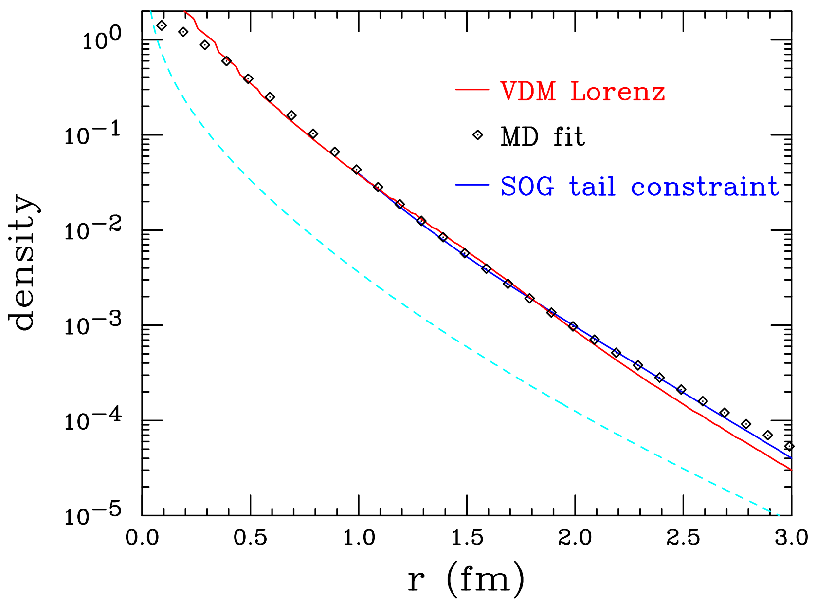
In Figure 12, we compare various densities: the Fourier transform of $G_e(q)$ (i.e., the density without relativistic corrections) of the MD fit, the density corresponding to the VDM fit of Lorenz et al.1 [85,119] (which includes the relativistic correction discussed in Section 3 in order to make it comparable) and the tail density of the SOG fit. While the large-r shape of the MD density and the density calculated from the $n{\pi }^{+}$ Fock state are very close, the tail of the VDM density falls somewhat more quickly, as a consequence of the low near-threshold strength of the spectral function.

A fit of the world data ($q_{max}$ = 10 fm${}^{-1}$) including two-photon corrections using the SOG density together with the tail constraint for $r>1.2$ fm yields [65] a charge rms-radius of $R=0.886\pm 0.008$ fm. The tail constraint is shown in Figure 12.

7. Summary

In this paper, we have discussed approaches used by various authors to extract the proton charge rms-radius R from data on elastic electron-proton scattering. We have pointed out the difficulties of the standard approach of fixing attention exclusively on the low-q data and the slope of the electric form factor $G_e(q)$ at $q=0$. The crux lies in the extrapolation from q’s, where the data are sensitive to R to $q=0$. The curvature of the parameterized $G_e(q)$’s needed for this extrapolation introduces a model dependence; the parametrizations in particular lack the physics constraint that the form factor is (with or without relativistic corrections) the Fourier transform of a density confined to a region in r of, say, $r<3$ fm.

We have emphasized that this curvature at low q is related to the shape of the charge density $\rho (r)$ at large radii r. About the latter quantity, we do have knowledge from physics, contrary to the curvature of $G(q)$ at low q; the density at large r is dominated by the least-bound Fock state of the proton, the ${\pi }^{+}n$ configuration. To obtain a reliable R, one must make sure that the density corresponding to $G(q)$ is reasonably close to this behavior.

This entails three consequences:

–

Use of a parameterized $G_e(q)$ that is physical, i.e., does indeed correspond to a density. This is not the case for most parameterizations employed in the literature.

–

Fit of the data to the largest $q_{max}$, in which case the data themselves fix to a fair degree the shape of $\rho (r)$ including its behavior at large r, hereby constraining the shape of $G_e(q)$ at low q.

–

Verification that $\rho (r)$ at large r shows a physical behavior and, better, use of a physical constraint to enforce the correct behavior. The fall-off given by the pion tail provides a very general and helpful physics constraint.

We have discussed a number of analyses of the e-p data that do respect the above insights. To determine the radius, we use the unweighted average of the (in part redone) fits: [3/5] Padé [91], dipole times polynomial in z [64], dipole times polynomial in $\xi$ [94], Bayesian inference [97], MD, Laguerre and SOG [65]. This yields a radius of:

$$\begin{array}{c}\hfill R=0.887\pm 0.012\mathrm{fm},\end{array}$$

(19)

where the error bar covers both the uncertainties of individual results, as well as their scatter. The results from the various analyses of e-p scattering that use physical parameterizations that lead to a sensible density at large r are quite compatible.

References

- Mohr, P.; Taylor, B.; Newell, D. CODATA Recommended Values of the Fundamental Physical Constants: 2010. Rev. Mod. Phys. 2012, 84, 1527. [Google Scholar] [CrossRef]
- Arrington, J.; Sick, I. Evaluation of the Proton Charge Radius from Electron-Proton Scattering. J. Phys. Chem. Ref. Data 2015, 44, 031204. [Google Scholar] [CrossRef]
- Pohl, R.; Antognini, A.; Nez, F.; Amaro, F.; Biraben, F.; Cardoso, J.M.R.; Covita, D.S.; Dax, A.; Dhawan, S.; Fernandes, L.M.P.; et al. The size of the proton. Nature 2010, 466, 213. [Google Scholar] [CrossRef] [PubMed]
- Pohl, R.; Nez, F.; Fernandes, L.M.P.; Amaro, F.D.; Biraben, F.; Cardoso, J.M.R.; Covita, D.S.; Dax, A.; Dhawan, S.; Diepold, M.; et al. Laser spectroscopy of muonic deuterium. Science 2016, 353, 669–673. [Google Scholar] [CrossRef] [PubMed]
- Peset, C.; Pineda, A. The Lamb shift in muonic hydrogen and the proton radius from effective field theories. Eur. Phys. J. A 2015, 51, 156. [Google Scholar] [CrossRef]
- Beyer, A.; Maisenbacher, L.; Matveev, A.; Pohl, R.; Khabarova, K.; Grinin, A.; Lamour, T.; Yost, D.C.; Hänsch, T.W.; Kolachevsky, N.; et al. The Rydberg constant and proton size from atomic hydrogen. Science 2017, 358, 79–85. [Google Scholar] [CrossRef] [PubMed]
- Fleurbaey, H. Frequency metrology of the 1S-3S transition of hydrogen: contribution to the proton charge radius puzzle. Available online: https://tel.archives-ouvertes.fr/tel-01633631 (accessed on 15 November 2017).
- Sick, I.; Trautmann, D. On the rms radius of the deuteron. Nucl. Phys. A 1998, 637, 559. [Google Scholar] [CrossRef]
- Rosenfelder, R. Coulomb corrections to elastic electron-proton scattering and the proton charge radius. Phys. Lett. B 2000, 479, 381. [Google Scholar] [CrossRef]
- Blunden, P.; Melnitchouk, W.; Tjon, J. Two-photon exchange in elastic electron-nucleon scattering. Phys. Rev. C 2005, 72, 034612. [Google Scholar] [CrossRef]
- Afanasev, A.; Blunden, P.; Hasell, D.; Raue, B. Two-photon exchange in elastic electron-proton scattering. Prog. Part. Nucl. Phys. 2017, 95, 245–278. [Google Scholar] [CrossRef]
- Rimal, D.; Adikaram, D.; Raue, B.A.; Weinstein, L.B.; Arrington, J.; Brooks, W.K.; Ungaro, M.; Adhikari, K.P.; Afanasev, A.V.; Akbar, Z.; et al. Measurement of two-photon exchange effect by comparing elastic e±p cross sections. Phys. Rev. C 2017, 95, 065201. [Google Scholar] [CrossRef]
- Rachek, I.A.; Arrington, J.; Dmitriev, V.F.; Gauzshtein, V.V.; Gerasimov, R.E.; Gramolin, A.V.; Holt, R.J.; Kaminskiy, V.V.; Lazarenko, B.A.; Mishnev, S.I.; et al. Measurement of the Two-Photon Exchange Contribution to the Elastic Scattering Cross Sections at the VEPP-3 Storage Ring. Phys. Rev. Lett. 2015, 114, 062005. [Google Scholar] [CrossRef] [PubMed]
- Henderson, B.S.; Ice, L.D.; Khaneft, D.; O’Connor, C.; Russell, R.; Schmidt, A.; Bernauer, J.C.; Kohl, M.; Akopov, N.; Alarcon, R.; et al. Hard Two-Photon Contribution to Elastic Lepton-Proton Scattering Determined by the OLYMPUS Experiment. Phys. Rev. Lett. 2017, 118, 092501. [Google Scholar] [CrossRef] [PubMed]
- Sick, I. On the rms-radius of the proton. Phys. Lett. B 2003, 576, 62–67. [Google Scholar] [CrossRef]
- Licht, A.; Pagnamenta, A. Wave Functions and Form Factors for Relativistic Composite Particles. I. Phys. Rev. D 1970, 2, 1150. [Google Scholar] [CrossRef]
- Mitra, A.; Kumari, I. Relativistic form factors for clusters with nonrelativistic wave functions. Phys. Rev. D 1977, 15, 261. [Google Scholar] [CrossRef]
- Ji, X. A relativistic skyrmion and its form factors. Phys. Lett. B 1991, 254, 456–461. [Google Scholar] [CrossRef]
- Kelly, J. Nucleon charge and magnetization densities from Sachs form factors. Phys. Rev. C 2002, 66, 065203. [Google Scholar] [CrossRef]
- Kelly, J. Simple parametrization of nucleon form factors. Phys. Rev. C 2004, 70, 068202. [Google Scholar] [CrossRef]
- Bumiller, F.; Croissiaux, M.; Dally, E.; Hofstadter, R. Electromagnetic Form Factors of the Proton. Phys. Rev. 1961, 124, 1623. [Google Scholar] [CrossRef]
- Janssens, T.; Hofstadter, R.; Hughes, E.; Yearian, M. Proton form factors from elastic electron-proton scattering. Phys. Rev. 1966, 142, 922. [Google Scholar] [CrossRef]
- Borkowski, F.; Peuser, P.; Simon, G.; Walther, V.; Wendling, R. Electromagnetic form factors of the proton at low four-momentum transfer. Nucl. Phys. A 1974, 222, 269–275. [Google Scholar] [CrossRef]
- Borkowski, F.; Simon, G.; Walther, V.; Wendling, R. Electromagnetic form factors of the peoton at low four-momentum transfer (II). Nucl. Phys. B 1975, 93, 461–478. [Google Scholar] [CrossRef]
- Simon, G.; Schmitt, C.; Borkowski, F.; Walther, V. Absolute electron-proton cross sections at low momentum transfer measured with a high pressure gas target system. Nucl. Phys. A 1980, 333, 381–391. [Google Scholar] [CrossRef]
- Simon, G.; Schmitt, C.; Walther, V. Elastic electric and magnetic e-d scattering at low momentum transfer. Nucl. Phys. A 1981, 364, 285–296. [Google Scholar] [CrossRef]
- Albrecht, W.; Behrend, H.; Brasse, F.; Flauger, W.; Hultschig, H.; Steffen, K.G. Elastic Electron-Proton Scattering at Momentum Transfers up to 245 F−2. Phys. Rev. Lett. 1966, 17, 1192. [Google Scholar] [CrossRef]
- Bartel, W.; Dudelzak, B.; Krehbiel, H.; McElroz, J.; Meyer-Berkhout, U.; Morrison, R.J.; Nguyen-Ngoc, H.; Schmidt, W.; Weber, G. Small-Angle Electron-Proton Elastic-Scattering Cross Sections for Squared Momentum Transfers Between 10 and 105 F−2. Phys. Rev. Lett. 1966, 17, 608. [Google Scholar] [CrossRef]
- Frerejacque, D.; Benaksas, D.; Drickey, D. Proton Form Factors from Observation of Recoil Protons. Phys. Rev. 1966, 141, 1308. [Google Scholar] [CrossRef]
- Albrecht, W.; Behrend, H.-J.; Dorner, H.; Flauger, W.; Hultschig, H. Some Recent Measurements of Proton Form Factors. Phys. Rev. Lett. 1967, 18, 1014. [Google Scholar] [CrossRef]
- Bartel, W.; Dudelzak, B.; Krehbiel, H.; McElroy, J.; Meyer-Berkhout, U.; Morrison, R.J.; Nguyen-Ngoc, H.; Schmidt, W.; Weber, G. The charge form factor of the proton at a momentum transfer of 75 F−2. Phys. Lett. B 1967, 25, 236. [Google Scholar] [CrossRef]
- Bartel, W.; Buesser, F.; Dix, W.; Felst, R.; Harms, D.; Krehbiel, H.; Kuhlmann, P.E.; McElroy, j.; Meyer, J.; Weber, G. Measurement of proton and neutron electromagnetic form factors at squared four-momentum transfers up to 3 (GeV/c)2. Nucl. Phys. B 1973, 58, 429–475. [Google Scholar] [CrossRef]
- Ganichot, D.; Grossetête, B.; Isabelle, D. Backward electron-deuteron scattering below 280 MeV. Nucl. Phys. A 1972, 178, 545–562. [Google Scholar] [CrossRef]
- Kirk, P.; Breidenbach, M.; Friedman, J.; Hartmann, G.; Kendall, H.; Buschhorn, G.; Coward, D.H.; DeStaebler, H.; Early, R.A.; Litt, J.; et al. Elastic Electron-Proton Scattering at Large Four-Momentum Transfer. Phys. Rev. D 1973, 8, 63. [Google Scholar] [CrossRef]
- Murphy, J.; Shin, Y.; Skopik, D. Proton form factor from 0.15 to 0.79 fm−2. Phys. Rev. C 1974, 9, 2125. [Google Scholar] [CrossRef]
- Berger, C.; Burkert, V.; Knop, G.; Langenbeck, B.; Rith, K. Electromagnetic form factors of the proton at squared four-momentum transfers between 10 and 50 fm−2. Phys. Lett. B 1971, 35, 87–89. [Google Scholar] [CrossRef]
- Bartel, W.; Buesser, F.W.; Dix, W.R.; Felst, R.; Harms, D.; Krehbiel, H.; Kuhlmann, P.E.; McElroy, J.; Weber, G. Electromagnetic proton form factors at squared four-momentum transfers between 1 and 3(GeV/c)2. Phys. Rev. Lett. 1970, 33, 245–248. [Google Scholar] [CrossRef]
- Borkowski, F.; Simon, G.; Walther, V.; Wendling, R. On the determination of the proton RMS-radius from electron scattering data. Z. Physik A 1975, 275, 29. [Google Scholar] [CrossRef]
- Bernauer, J.; Achenbach, P.; Gayoso, C.A.; Böhm, R.; Bosnar, D.; Debenjak, L.; Distler, M.O.; Doria, L.; Esser, A.; Fonvieille, H.; et al. High-Precision Determination of the Electric and Magnetic Form Factors of the Proton. Phys. Rev. Lett. 2010, 105, 242001. [Google Scholar] [CrossRef] [PubMed]
- Amroun, A. Mesure Des Facteurs De Forme Electromagnetiques Des Noyaux Helium-3 Et Tritium Par Diffusion D’electrons. Ph.D. Thesis, Université de Bordeaux, Bordeaux, France, 1989. [Google Scholar]
- Dudelzak, B.; Sauvage, G.; Lehmann, P. Measurements of the form factors of the proton at momentum transfers q22 fermi−2. Nuov. Cim. 1963, 28, 18–24. [Google Scholar] [CrossRef]
- Qattan, I.; Arrington, J.; Segel, R.; Zheng, X.; Aniol, K.; Baker, O.K.; Beams, R.; Brash, E.J.; Calarco, J.; Camsonne, A.; et al. Precision Rosenbluth Measurement of the Proton Elastic Form Factors. Phys. Rev. Lett. 2005, 94, 142301. [Google Scholar] [CrossRef] [PubMed]
- Christy, M.E.; Ahmidouch, A.; Armstrong, C.S.; Arrington, J.; Asaturyan, R.; Avery, S.; Baker, O.; Beck, D.; Blok, H.P.; Bochna, C.W.; et al. Measurements of electron-proton elastic cross sections for 0.4 < Q2 < 5.5 (GeV/c)2. Phys. Rev. C 2004, 70, 015206. [Google Scholar]
- Dutta, D.; Van Westrum, D.; Abbott, D.; Ahmidouch, A.; Amatuoni, T.A.; Armstrong, C.; Arrington, J.; Assamagan, K.A.; Bailey, K.; Baker, O.K.; et al. Quasielastic (e,e′p) reaction on 12C, 56Fe, and 197Au. Phys. Rev. C 2003, 68, 064603. [Google Scholar] [CrossRef]
- Niculescu, I.; Armstrong, C.; Arrington, J.; Assamagan, K.; Baker, O.; Beck, D.H.; Bochna, C.W.; Carlini, R.D.; Cha, J.; Cothran, C.; et al. Evidence for valencelike quark-hadron duality. Phys. Rev. Lett. 2000, 85, 1182. [Google Scholar] [CrossRef] [PubMed]
- Rock, S.; Arnold, R.; Bosted, P.; Chertok, B.; Mecking, B.; Schmidt, I.; Szalata, Z.M.; York, R.C.; Zdarko, R. Measurement of elastic electron-neutron scattering and inelastic electron-deuteron scattering cross sections at high momentum transfer. Phys. Rev. D 1992, 46, 24. [Google Scholar] [CrossRef]
- Stein, S.; Atwood, W.; Bloom, E.; Cottrell, R.; DeStaebler, H.; Jordan, C.L.; Piel, H.G.; Prescott, C.Y.; Siemann, R.; Taylor, R.E.; et al. Electron scattering at 4∘ with energies of 4.5–20 GeV. Phys. Rev. D 1975, 12, 1884. [Google Scholar] [CrossRef]
- Goitein, M.; Budnitz, R.; Carroll, L.; Chen, J.; Dunning, J.; Hanson, K.; Imrie, D.C.; Mistretta, C.; Wilson, R. Elastic Electron-Proton Scattering Cross Sections Measured by a Coincidence Technique. Phys. Rev. D 1970, 1, 2449. [Google Scholar] [CrossRef]
- Bosted, P.; Katramatou, A.; Arnold, R.; Benton, D.; Clogher, L.; DeChambrier, G.; Lambert, J.; Lung, A.; Petratos, G.G.; Rahbar, A.; et al. Measurements of the deuteron and proton magnetic form factors at large momentum transfers. Phys. Rev. C 1990, 42, 38. [Google Scholar] [CrossRef]
- Bosted, P.E.; Andivahis, L.; Lung, A.; Stuart, L.M.; Alster, J.; Arnold, R.G.; Chang, C.C.; Dietrich, F.S.; Dodge, W.; Gearhart, R.; et al. Measurements of the electric and magnetic form factors of the proton from Q2 = 1.75 to 8.83 (GeV/c)2. Phys. Rev. Lett. 1992, 68, 3841–3844. [Google Scholar] [CrossRef] [PubMed]
- Sill, A. Jailbar optical studies of the SLAC 8-GeV/c spectrometer. Available online: http://inspirehep.net/record/243145/ (accessed on 10 November 2017).
- Price, L.E.; Dunning, J.R.; Goitein, M.; Hanson, K.; Kirk, T.; Wilson, R. Backward-angle electron-proton elastic scattering and proton electromagnetic form factors. Phys. Rev. D 1971, 4, 45. [Google Scholar] [CrossRef]
- Litt, J.; Buschhorn, G.; Coward, D.; Destaebler, H.; Mo, L.; Taylor, R.E.; Barish, B.C.; Loken, S.C.; Pine, J.; Friedman, J.I.; et al. Measurement of the ratio of the proton form factors, GE/GM, at high momentum transfers and the question of scaling. Phys. Lett. B 1970, 31, 40–44. [Google Scholar] [CrossRef]
- Walker, R.; Filippone, B.; Jourdan, J.; Milner, R.; McKeown, R.; Potterveld, D.; Arnold, R.; Benton, D.; Bosted, P.; Clogher, L.; et al. Measurement of the proton elastic form factors for Q2 = 1–3 (Gev/c)2. Phys. Lett. B 1989, 224, 353–358. [Google Scholar] [CrossRef]
- Walker, R.; Filippone, B.; Jourdan, J.; Milner, R.; McKeown, R.; Potterveld, D.; Andivahis, L.; Arnold, R.; Benton, D.; Bosted, P.; et al. Measurements of the proton elastic form factors for 1 ≤ Q2 ≤ 3 (GeV/c)2 at SLAC. Phys. Rev. D 1994, 49, 5671. [Google Scholar] [CrossRef]
- Andivahis, L.; Bosted, P.E.; Lung, A.; Stuart, L.M.; Alster, J.; Arnold, R.G.; Chang, C.C.; Dietrich, F.S.; Dodge, W.; Gearhart, R.; et al. Measurements of the electric and magnetic form factors of the proton from Q2 = 1.75 to 8.83 (GeVc)2. Phys. Rev. D 1994, 50, 5491. [Google Scholar] [CrossRef]
- Drickey, D.; Hand, L. Precise Neutron and Proton Form Factors at Low Momentum Transfers. Phys. Rev. Lett. 1962, 9, 521. [Google Scholar] [CrossRef]
- Punjabi, V.; Perdrisat, C.F.; Aniol, K.A.; Baker, F.T.; Berthot, J.; Bertin, P.Y.; Bertozzi, W.; Besson, A.; Bimbot, L.; Boeglin, W.U.; et al. Proton elastic form factor ratios to Q2 = 3.5 GeV2 by polarization transfer. Phys. Rev. C 2005, 71, 055202. [Google Scholar] [CrossRef]
- Gayou, O.; Wijesooriya, K.; Afanasev, A.; Amarian, M.; Aniol, K.; Becher, S.; Benslama, K.; Bimbot, L.; Bosted, P.; Brash, E.; et al. Measurements of the elastic electromagnetic form factor ratio μp GEp/GMp via polarization transfer. Phys. Rev. C 2001, 64, 038202. [Google Scholar] [CrossRef]
- Gayou, O.; Aniol, K.A.; Averett, T.; Benmokhtar, F.; Bertozzi, W.; Bimbot, L.; Brash, E.J.; Calarco, J.R.; Cavata, C.; Chai, Z.; et al. Measurement of GEp/GMp in p → to Q2 = 5.6 GeV2. Phys. Rev. Lett. 2002, 88, 092301. [Google Scholar] [CrossRef] [PubMed]
- Zhan, X.; Allada, K.; Armstrong, D.; Arrington, J.; Bertozzi, W.; Boeglin, W.; Chen, J.P.; Chirapatpimol, K.; Choi, S.; Chudakov, E.; et al. High-precision measurement of the proton elastic form factor ratio μpGE/GM at low Q2. Phys. Lett. B 2011, 705, 59–64. [Google Scholar] [CrossRef]
- Botterill, D.; Braben, D.; Montgomery, H.; Norton, P.; Matone, G.; Del Guerra, A.; Giazotto, A.; Giorgi, M.A.; Orsitto, F.; Stefaninia, A. Elastic electron-proton scattering between 0.05 and 0.30 (GeV/c)2. Phys. Lett. B 1973, 46, 125–128. [Google Scholar] [CrossRef]
- Bernauer, J. Measurement of the elastic electron-proton cross section and separation of the electric and magnetic form factor in the Q2 range from 0.004 to 1 (GeV/c)2. Available online: http://wwwa1.kph.uni-mainz.de/A1/publications/doctor/bernauer.pdf (accessed on 12 November 2017).
- Lee, G.; Arrington, J.; Hill, R. Extraction of the proton radius from electron-proton scattering data. Phys. Rev. D 2015, 92, 013013. [Google Scholar] [CrossRef]
- Sick, I. Problems with proton radii. Prog. Part. Nucl. Phys. 2012, 67, 473–478. [Google Scholar] [CrossRef]
- Mo, L.; Tsai, Y. Radiative Corrections to Elastic and Inelastic ep and up Scattering. Rev. Mod. Phys. 1969, 41, 205. [Google Scholar] [CrossRef]
- Maximon, L.; Tjon, J. Radiative corrections to electron-proton scattering. Phys. Rev. C 2000, 62, 054320. [Google Scholar] [CrossRef]
- Strauch, S.; Dieterich, S.; Aniol, K.A.; Annand, J.R.M.; Baker, O.K.; Bertozzi, W.; Boswell, M.; Brash, E.J.; Chai, Z.; Chen, J.P.; et al. Polarization Transfer in the 4He (, e’)3H Reaction up to Q2 = 2.6 (GeV/c)2. Phys. Rev. Lett. 2003, 91, 052301. [Google Scholar] [CrossRef] [PubMed]
- Milbrath, B.; McIntyre, J.; Armstrong, C.; Barkhuff, D.; Bertozzi, W.; Chen, J.P.; Dale, D.; Dodson, G.; Dow, K.A.; Epstein, M.B.; et al. Comparison of Polarization Observables in Electron Scattering from the Proton and Deuteron. Phys. Rev. Lett. 1998, 80, 452. [Google Scholar] [CrossRef]
- Pospischil, T.; Bartsch, P.; Baumann, D.; Bermuth, J.; Böhm, R.; Bohinc, K.; Derber, S.; Ding, M.; Distler, M.; Drechsel, D.; et al. Measurement of the Recoil Polarization in the p (, e’ ) π 0 Reaction at the Δ (1232) Resonance. Phys Rev. Lett. 2001, 86, 2959. [Google Scholar] [CrossRef] [PubMed]
- Crawford, C.B.; Sindile, A.; Akdogan, T.; Alarcon, R.; Bertozzi, W.; Booth, E.; Botto, T.; Calarco, J.; Clasie, B.; DeGrush, A.; et al. Measurement of the Proton’s Electric to Magnetic Form Factor Ratio from (,e’p). Phys. Rev. Lett. 2007, 98, 052301. [Google Scholar] [CrossRef] [PubMed]
- Ron, G.; Glister, J.; Lee, B.; Allada, K.; Armstrong, W.; Arrington, J.; Beck, A.; Benmokhtar, F.; Berman, B.L.; Boeglin, W.; et al. Measurements of the Proton Elastic-Form-Factor Ratio mu pG p E/G p M at Low Momentum Transfer. Phys. Rev. Lett. 2007, 99, 202002. [Google Scholar] [CrossRef] [PubMed]
- MacLachlan, G.; Aghalaryan, A.; Ahmidouch, A.; Anderson, B.D.; Asaturyan, R.; Baker, O.; Baldwin, A.R.; Barkhuff, D.; Breuer, H.; Carlini, R.; et al. The ratio of proton electromagnetic form factors via recoil polarimetry at Q2 = 1.13 (GeV/c)2. Nucl. Phys. A 2006, 764, 261–273. [Google Scholar] [CrossRef]
- Jones, M.K.; Aniol, K.A.; Baker, F.T.; Berthot, J.; Bertin, P.Y.; Bertozzi, W.; Besson, A.; Bimbot, L.; Boeglin, W.U.; Brash, E.J.; et al. GEp/GMp Ratio by Polarization Transfer in p→ . Phys. Rev. Lett. 2000, 84, 1398. [Google Scholar] [CrossRef] [PubMed]
- Jones, M.K.; Aghalaryan, A.; Ahmidouch, A.; Asaturyan, R.; Bloch, F.; Boeglin, W.; Bosted, P.; Carasco, C.; Carlini, R.; Cha, J.; et al. Proton GE/GM from beam-target asymmetry. Phys. Rev. C 2006, 74, 035201. [Google Scholar] [CrossRef]
- Puckett, A.J.R.; Brash, E.J.; Jones, M.K.; Luo, W.; Meziane, M.; Pentchev, L.; Perdrisat, C.F.; Punjabi, V.; Wesselmann, F.R.; Abdellah, A.; et al. Recoil Polarization Measurements of the Proton Electromagnetic Form Factor Ratio to Q2 = 8.5 GeV2. Phy. Rev. Lett. 2010, 104, 242301. [Google Scholar] [CrossRef] [PubMed]
- Puckett, A.J.R.; Brash, E.J.; Gayou, O.; Jones, M.K.; Pentchev, L.; Perdrisat, C.F.; Punjabi, V.; Aniol, K.A.; Averett, T.; Benmokhtar, F.; et al. Final analysis of proton form factor ratio data at Q2 = 4.0, 4.8, and 5.6 GeV2. Phys. Rev. C 2012, 85, 045203. [Google Scholar]
- Dieterich, S.; Bartsch, P.; Baumann, D.; Böhm, J.B.R.; Bohinc, K.; Böhm, R.; Bosnar, D.; Derber, S.; Ding, M.; Distler, M.; et al. Polarization transfer in the 4He (e→, e’p→)3 H reaction. Phys. Lett. B 2001, 500, 47–52. [Google Scholar] [CrossRef]
- Paolone, M.; Malace, S.P.; Strauch, S.; Albayrak, I.; Arrington, J.; Berman, B.L.; Brash, E.J.; Briscoe, B.; Camsonne, A.; Chen, J.P.; et al. Polarization Transfer in the 4He(,e’)3H Reaction at Q2 = 0.8 and 1.3 (GeV/c)2. Phys. Rev. Lett. 2010, 105, 072001. [Google Scholar] [CrossRef] [PubMed]
- Friar, J.; Sick, I. Zemach moments for hydrogen and deuterium. Phys. Lett. B 2004, 579, 285–289. [Google Scholar] [CrossRef]
- Friar, J.; Sick, I. Muonic hydrogen and the third Zemach moment. Phys. Rev. A 2005, 72, 040502. [Google Scholar] [CrossRef]
- Horbatsch, M.; Hessels, E. Evaluation of the strength of electron-proton scattering data for determining the proton charge radius. Phys. Rev. C 2016, 93, 015204. [Google Scholar] [CrossRef]
- Higinbotham, D.; Kabir, A.; Lin, V.; Meekins, D.; Norum, B.; Sawatzky, B. Proton radius from electron scattering data. Phys. Rev. C 2016, 93, 055207. [Google Scholar] [CrossRef]
- Griffioen, K.; Carlson, C.; Maddox, S. Consistency of electron scattering data with a small proton radius. Phys. Rev. C 2016, 93, 065207. [Google Scholar] [CrossRef]
- Lorenz, I.; Meissner, U.G. Reduction of the proton radius discrepancy by 3σ. Phys. Lett. B 2014, 737, 57–59. [Google Scholar] [CrossRef] [Green Version]
- Sick, I.; Trautmann, D. Proton root-mean-square radii and electron scattering. Phys. Rev. C 2014, 89, 012201(R). [Google Scholar] [CrossRef]
- Sick, I. Importance of Tail of Proton Density. Few-Body Syst. 2014, 55, 903. [Google Scholar] [CrossRef]
- Sick, I.; Trautmann, D. Reexamination of proton rms radii from low-q power expansions. Phys. Rev. C 2017, 95, 012501. [Google Scholar] [CrossRef]
- Gasparian, A.; Pedroni, R.; Ahmed, A.; Khandaker, M.; Punjabi, V.; Salgado, v.; Akushevich, I.; Gao, H.; Huang, M.; Laskaris, G.; et al. High precision measurement of the proton charge radius. Available online: https://pdfs.semanticscholar.org/06d6/1cc255edb67eb9adccf3605dd313eaff5504.pdf (accessed on 26 November 2017).
- Bernauer, J.; Distler, M.; Friedrich, J.; Walcher, T.; Achenbach, P.; Ayerbe Gayoso, C.; Böhm, R.; Bosnar, D.; Debenjak, L.; Doria, L.; et al. Electric and magnetic form factors of the proton. Phys. Rev. C. 2014, 90, 015206. [Google Scholar] [CrossRef]
- Arrington, J.; Melnitchouk, W.; Tjon, J. Global analysis of proton elastic form factor data with two-photon exchange corrections. Phys. Rev. C 2007, 76, 035205. [Google Scholar] [CrossRef]
- Kraus, E.; Mesick, K.; White, A.; Gilman, R.; Strauch, S. Polynomial fits and the proton radius puzzle. Phys. Rev. C 2014, 90, 045206. [Google Scholar] [CrossRef]
- Hill, R.; Paz, G. Model-independent extraction of the proton charge radius from electron scattering. Phys. Rev. D 2010, 82, 113005. [Google Scholar] [CrossRef]
- Borisyuk, D. Proton charge and magnetic rms radii from the elastic ep scattering data. Nucl. Phys. A 2010, 843, 59–67. [Google Scholar] [CrossRef]
- Friar, J. Relativistic corrections to electron scattering by 2He, 3He, and 4He. Ann. Phys. 1973, 81, 332–363. [Google Scholar] [CrossRef]
- Anni, R.; Có, G.; Pellegrino, P. Nuclear charge density distributions from elastic electron scattering data. Nucl. Phys. A 1995, 584, 35–39. [Google Scholar] [CrossRef]
- Graczyk, K.; Juszczak, C. Proton radius from Bayesian inference. Phys. Rev. C 2014, 90, 054334. [Google Scholar] [CrossRef]
- Sick, I. Model-independent nuclear charge densities from elastic electron scattering. Nucl. Phys. A 1974, 218, 509–541. [Google Scholar] [CrossRef]
- Iachello, F.; Jackson, A.; Lande, A. Semi-phenomenological fits to nucleon electromagnetic form factors. Phys. Lett. B 1973, 43, 191–196. [Google Scholar] [CrossRef]
- Blatnik, S.; Zovko, N. Nucleon form factors in the extended VDM supplemented with asymptotic constraints. Acta Phys. Austriaca 1974, 39, 62. [Google Scholar]
- Gari, M.; Krümpelmann, W. The electric neutron form factor and the strange quark content of the nucleon. Phys. Lett. B 1992, 274, 159–162. [Google Scholar] [CrossRef]
- Lomon, E. Extended Gari-Krümpelmann model fits to nucleon electromagnetic form factors. Phys. Rev. C 2001, 64, 035204. [Google Scholar] [CrossRef]
- Bijker, R.; Iachello, F. Reanalysis of the nucleon spacelike and timelike electromagnetic form factors in a two-component model. Phys. Rev. C 2004, 69, 068201. [Google Scholar] [CrossRef]
- Bernauer, J.; Distler, M. Avoiding common pitfalls and misconceptions in extractions of the proton radius. arXiv, 2016; arXiv:1606.02159. [Google Scholar]
- Lorenz, I.; Hammer, H.W.; Meissner, U.G. The size of the proton: Closing in on the radius puzzle. Eur. Phys. J. A 2012, 48, 151. [Google Scholar] [CrossRef]
- Graczyk, K.; Plonski, P.; Sulei, R. Neural network parameterizations of electromagnetic nucleon form-factors. arXiv, 2010; arXiv:1006.0342. [Google Scholar]
- Gari, M.; Krümpelmann, W. Semiphenomenological synthesis of meson and quark dynamics and the E.M. structure of the nucleon. Z. Phys. 1985, 322, 689. [Google Scholar] [CrossRef]
- Mergell, P.; Meissner, U.G.; Drechsel, D. Dispersion-theoretical analysis of the nucleon electromagnetic form factors. Nucl. Phys. A 1996, 596, 367–396. [Google Scholar] [CrossRef]
- Hammer, H.W.; Drechsel, D.; Meissner, U.G. On the pion cloud of the nucleon. Phys. Lett. B 2004, 586, 291–296. [Google Scholar] [CrossRef] [Green Version]
- Lorenz, I.; Meissner, U.G.; Hammer, H.W.; Dong, Y. Theoretical constraints and systematic effects in the determination of the proton form factors. Phys. Rev. D 2015, 91, 014023. [Google Scholar] [CrossRef]
- Höhler, G.; Pietarinen, E.; Sabba-Stefanescu, I.; Borkowski, F.; Simon, G.; Walther, V.H.; Wendling, R.D. Analysis of electromagnetic nucleon form factors. Nucl. Phys. B 1976, 114, 505–534. [Google Scholar] [CrossRef]
- Höhler, G.; Pietarinen, E. Electromagnetic radii of nucleon and pion. Phys. Lett. B 1975, 53, 471–475. [Google Scholar] [CrossRef]
- Höhler, G. Landolt-Boernstein, Springer: Berlin, Germany, 1983; Volume 9.
- Adamuscin, C.; Dubnicka, S.; Dubnickova, A. New value of the proton charge root mean square radius. Prog. Part. Nucl. Phys. 2012, 67, 479–485. [Google Scholar] [CrossRef]
- Alarcon, J.; Weiss, C. Nucleon form factors in dispersively improved Chiral Effective Field Theory II: Electromagnetic form factors. arXiv, 2017; arXiv:1710.06430v1. [Google Scholar]
- Horbatsch, M.; Hessels, E.; Pineda, A. Proton radius from electron-proton scattering and chiral perturbation theory. Phys. Rev. C 2017, 95, 035203. [Google Scholar] [CrossRef]
- Sick, I. Precise root-mean-square radius of 4He. Phys. Rev. C 2008, 77, 041302. [Google Scholar] [CrossRef]
- Sick, I. Precise nuclear radii from electron scattering. Phys. Lett. B 1982, 116, 212–214. [Google Scholar] [CrossRef]
- Lorenz, I. Private communication, 2012.