Mixed Basis Sets for Atomic Calculations

Abstract

Many numerical methods of atomic calculations use one-electron basis sets. These basis sets must meet rather contradictory requirements. On the one hand, they must include physically justified orbitals, such as Dirac–Fock ones, for the one-electron states with high occupation numbers. On the other hand, they must ensure rapid convergence of the calculations in respect to the size of the basis set. It is difficult to meet these requirements using a single set of orbitals, while merging different subsets may lead to linear dependence and other problems. We suggest a simple unitary operator that allows such merging without aforementioned complications. We demonstrated robustness of the method on the examples of Fr and Au.

1. Introduction

Many methods of atomic calculations, such as configuration interaction (CI) and many-body perturbation theory (MBPT), use basis sets of one-electron orbitals. Other methods use some combinations of CI and MBPT and also require basis sets. In particular, the CI+MBPT method [1] uses CI for valence electrons, where correlations are strong, and accounts for weaker core–valence correlations by means of the MBPT. The method is rather flexible and can be applied for any atom with few valence electrons and arbitrary large core. For CI+MBPT calculations, we use computer package [2], which is based on the Dirac–Fock code [3]. There are several other packages, which use slightly different variants of the same CI+MBPT method [4,5,6], or its generalization [7].

In the CI+MBPT method, we use Dirac–Fock orbitals for all core and valence orbitals of an atom. Then, we add virtual orbitals to form a more, or less complete basis set. The difference between valence and virtual orbitals is that the latter have small occupation numbers in the physical atomic states of interest. Virtual states may be chosen rather arbitrarily, with some not very well defined requirements of ‘usefulness’ and ‘completeness’. It is important though to have a regular way to increase the size of the basis set and study convergence of the calculations.

Because of the existence of the defused Rydberg states and the continuum spectrum, it is usually ineffective to use eigenfunctions of the one-electron Hamiltonian as virtual orbitals. Instead, one of the common choices for the virtual orbitals are B-splines [8,9]. However, sometimes it is necessary to use very large basis sets of B-splines to get high accuracy results. This happens, for example, for calculations of the parity nonconservation effects and the hyperfine constants in heavy atoms. The size of the basis set can be significantly reduced by adding the Dirac–Fock orbitals of occupied and weakly excited (valence) one-electron states. The problem one meets in this case is to exclude B-splines which are linear dependent with these Dirac–Fock orbitals. Here, we discuss a method to form an orthogonal basis set from two different subsets using a unitary operator suggested by Abarenkov and Tupitsyn [10] for other purposes. This method is not specific to B-splines, but can be used for other basis sets, such as, for example, the Dirac–Fock–Sturm basis set [11]. We use atomic units $\hslash =e=m_e=1$ throughout the paper.

2. Method

The basis set for atomic calculations consists of subsets for different partial waves, which are defined by the relativistic quantum number $\varkappa =(l-j)(2j+1)$, where l and j are orbital and total angular momenta. These subsets are independent and within each subset the orbitals must be orthogonal and normalized to unity. Let us consider one partial wave and assume that it includes n Dirac–Fock orbitals ${\psi }_p$. These orbitals are defined on the radial grid [3]. On the same grid, one can form a set of k B-splines $B_q$ ($k>n$). The set of splines is ‘complete’ in the sense that their sum for all grid points is equal to unity (if we want B-splines to turn to zero at the boundaries, then this is true only for the grid points sufficiently far from the edges).

Let us assume for simplicity that B-splines are orthogonalized using, for example, the Löwdin method [12,13]. If we add these k splines to n Dirac–Fock orbitals, we get a set with strong linear dependence, which can not be effectively orthogonalized and will include nonphysical orbitals, not useful for calculations. Instead, we want to form $(k-n)$ new virtual orbitals ${\psi }_r$, $r=n+1,\dots ,k$ which can be added to the existing set of n physical ones.

Up to now, we ignored lower components of the radial Dirac–Fock orbitals. Calculations for many-electron atoms are usually done in the no-virtual-pair approximation when a negative continuum is neglected. Then, the simplest way to treat lower components sufficiently accurately and avoid problems with nonphysical ‘intruder’ states is to use B-spline expansion only for the upper components and add a lower component to each B-spline using a kinetic balance method [14]. Alternatively, one can use a dual kinetic balance method [15], which is particularly useful for QED calculations. Below, we use the term B-spline to the two-component radial orbital where the upper component is B-spline $B_q$ and the lower component $L_q$ is found from the kinetic balance condition:

$$\begin{array}{cc}\hfill L_q& =\frac{-\alpha }{2}\left(\frac{d}{dr}+\frac{\varkappa }{r}\right)B_q,\hfill \end{array}$$

(1)

where $\alpha$ is the fine structure constant.

For the orbitals defined on the radial grid it is easy to improve kinetic balance approximation by including the dominant term of the potential energy, i.e., interaction with the nucleus:

$$\begin{array}{cc}\hfill L_q& =\frac{-\alpha }{2+{\alpha }^{2}Z/r}\left(\frac{d}{dr}+\frac{\varkappa }{r}\right)B_q,\hfill \end{array}$$

(2)

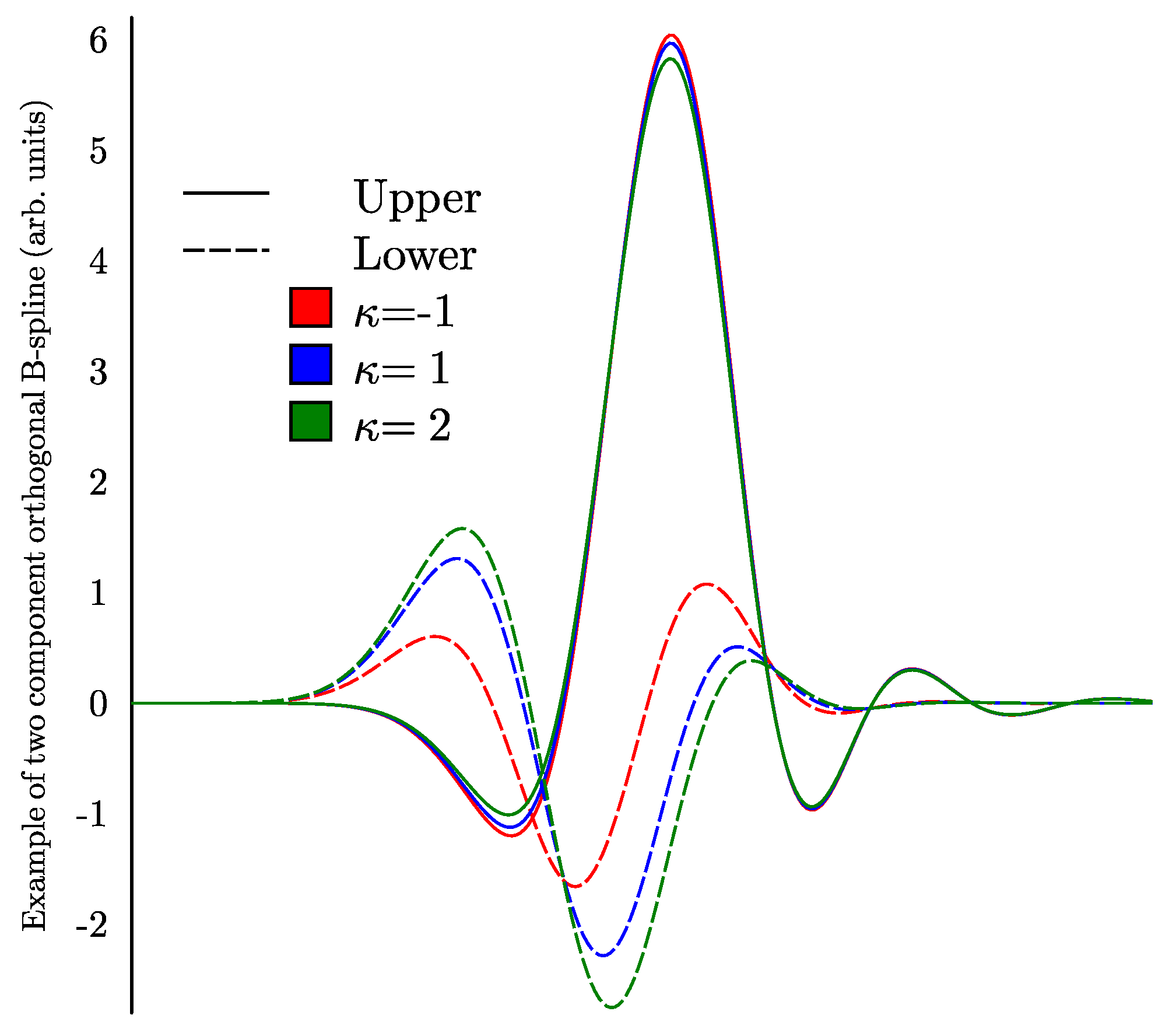
where Z is the nuclear charge. Expressions (1) and (2) are very close at the distances $r\sim 1$, but at the distances $r\lesssim \alpha$ the difference becomes large and Equation (2) works better. Here, we form lower components using Equation (2) instead of the more conventional Equation (1). Figure 1 shows the same two-component B-spline for Fr ($Z=87$) from a set of orthonormal B-splines of rank 7 for different values of $\varkappa$. Note that such two-component B-splines depend on parameters Z and $\varkappa$ (the large component depends on these parameters because of the orthogonalization).

Now, we shortly describe how to form an orthogonal basis set from two different subsets using specially designed unitary operator. Let us calculate an overlap matrix

$$\begin{array}{c}\hfill S_{pq}=\langle {\psi }_p|B_q\rangle \end{array}$$

(3)

and find n B-splines that have maximum projections on the physical orbitals ${\psi }_p$:

$$\begin{array}{ccc}\hfill & B_{q_p}\leftrightarrow {\psi }_p,\hfill & \hfill p=1\dots n.\end{array}$$

(4)

Suppose now that we have a unitary operator U which converts each of these n B-splines into respective orbital ${\psi }_p$:

$$\begin{array}{ccc}\hfill & {\alpha }_p{\psi }_p=U{B}_{q_p},\hfill & \hfill {\alpha }_p=\pm 1,\end{array}$$

(5)

where the phase factor ${\alpha }_p$ will be discussed later. If we apply this operator to the whole set of B-splines, we get a set of k orthonormal orbitals ${\psi }_q$ which includes n initial orbitals and has similar completeness as the set of B-splines.

A simple and convenient variant of the operator we are looking for was suggested in Ref. [10]. It has a following form:

$$\begin{array}{cc}\hfill & U=I-R,\hfill \\ \hfill & R=\sum _{p^{\prime },p=1}^n|{\chi }_p^{\prime }\rangle Q_{p^{\prime }p}^{-1}\langle {\chi }_p|,\hfill \\ \hfill & {\chi }_p=B_{q_p}-{\alpha }_p{\psi }_p,\hfill \\ \hfill & Q_{p^{\prime }p}=\langle {\chi }_{p^{\prime }}|B_{q_p}\rangle ={\delta }_{p^{\prime }p}-{\alpha }_{p^{\prime }}{S}_{p^{\prime }{q}_p},\hfill \end{array}$$

(6)

and matrix S is defined by Equation (3).

The phase factors ${\alpha }_p$ in Equation (6) comes from definition (5). It was introduced in Ref. [10] to add more flexibility. For example, this phase factor allows for avoiding problems when $B_{q_p}$ and ${\psi }_p$ are very close and ${\chi }_p$ may be poorly defined for ${\alpha }_p=1$. We do not seem to have this problem here because B-splines do not resemble physical orbitals too closely. However, it may be useful to see how the basis set depends on the choice of this phase.

The procedure described above allows one to form an orthonormal basis set where n B-splines are replaced by n Dirac–Fock orbitals. Other B-splines are orthogonalized to Dirac–Fock orbitals and to each other. This orthogonalization is equivalent to the procedure described in Ref. [16]. Our method relies on the unitarity of operator (6). In Ref. [10], this operator was proven to be unitary if n orbitals ${\psi }_p$ and n B-splines $B_{q_n}$ are linearly independent. Formally, this condition is always satisfied if the number of grid points is much bigger than the total number of orbitals $n+k$. However, when n is approaching the number of splines k, this set of $2n$ functions becomes more and more linear dependent. As a result, the loss of orthogonality occurs between the orbitals generated with the help of the operator U. Below, we will see that the quality of the basis set may be improved by proper choice of the phase factor ${\alpha }_p$.

3. Test Calculations

In this section, we use the method described above to generate different basis sets for Fr ($Z=87$) and Au ($Z=79$). We study how these basis sets depend on the choice of the phase factor ${\alpha }_p$ in Equation (5). We also make test MBPT calculations for Au and study convergence of the results for the binding energies and the hyperfine constants with the number of B-splines.

3.1. An Example of Fr Atom

Here, we generate different basis sets for Fr ([Rn]7s) using the method described above. This atom has a large Rn-like core $[1s^2\dots 6s^{2}6p^6]$ with 24 relativistic subshells. All core orbitals are found by solving Dirac–Fock equations for the $V^{N-1}$ potential. Then, we form several valence orbitals in the same $V^{N-1}$ potential. For the partial wave $s_{1/2}$ we end up with six core orbitals $1s$–$6s$ and three valence orbitals $7s$–$9s$.

Now, we try to construct virtual s orbitals with the help of relatively small set of B-splines. We form 20 orthogonal two-component B-splines of rank 5 and construct unitary operator U defined in Equation (6). Applying this operator to the splines (5), we reproduce all nine Dirac–Fock orbitals $1s$–$9s$ plus 11 additional virtual orbitals. Three of these orbitals are localized very close to the nucleus, closer than a $1s$ orbital. These orbitals can be excluded from the basis set, unless we are interested in such atomic properties, as hyperfine structure, which strongly depends on the wave functions near the origin. Five virtual orbitals are localized in the core region between $1s$ and $6s$. The remaining three orbitals are localized in the valence region. Together, these eight orbitals are useful for treating core–valence correlations.

Using a set of 40 orthogonal splines, we can construct 31 virtual orbitals: 11 of them are localized close to the origin, another 11 in the core region, and 9 virtual orbitals in the valence region. Changing the number of splines, we can form different basis sets and study convergence. It is important that, in all basis sets, the Dirac–Fock orbitals are unchanged. This is not the case if all orbitals are expanded in B-splines and original orbitals are substituted by their expansions. This requires much longer sets of B-splines to avoid significant deterioration of the core and valence orbitals. It is most difficult to accurately reproduce physical orbitals with B-splines near the origin. This is important when we are interested in calculating parity non-conserving interactions, the isotope shifts, or the hyperfine structure.

The number of Dirac–Fock orbitals depends on the partial wave. For higher partial waves, we have a smaller number of Dirac–Fock orbitals and, therefore, can form more virtual orbitals using the same set of splines. We generated basis sets of different length using B-splines of the ranks from 4 to 7. We used from 15 to 46 B-splines per partial wave. In each case, we were able to construct unitary operator (6) and produce orthonormal joint basis set of B-splines and Dirac–Fock orbitals. At present, we are using some of these basis sets to calculate magnetic hyperfine structure constants and to study the hyperfine anomaly for short-lived isotopes of Fr. Results of this work will be published elsewhere.

3.2. An Example of Au Atom: Spectrum

Now, we are going to study how the generated basis set depends on the choice of the phase factor ${\alpha }_p$ in Equation (5). It is natural to assume that the optimal choice of the phase should depend on the sign of the scalar product $\langle {\psi }_p|B_{q_p}\rangle \equiv S_{p{q}_p}$. Therefore, we compare two variants

$$\begin{array}{cc}\hfill & {\alpha }_p^{(\pm )}=\pm \mathrm{sign}\left(S_{p{q}_p}\right).\hfill \end{array}$$

(7)

We will designate basis sets generated with these two phase conventions as ${\mathsf{\Pi }}_{+}$ and ${\mathsf{\Pi }}_{-}$, respectively.

As an example, we have chosen a neutral Au, which has 78 electrons in 21 closed relativistic subshells $1s_{1/2}\dots 5d_{5/2}$ and one unpaired electron. The Dirac–Fock equations are solved for the $V^{N-1}$ potential. Then, we use 15 orthogonal B-splines from the set of 20 splines of rank 5 to generate eight virtual orbitals with two phase conventions (7). As we mentioned at the end of Section 2, this is a potentially dangerous situation as the number of splines is comparable to the number of physical orbitals and we can expect significant linear dependence between them.

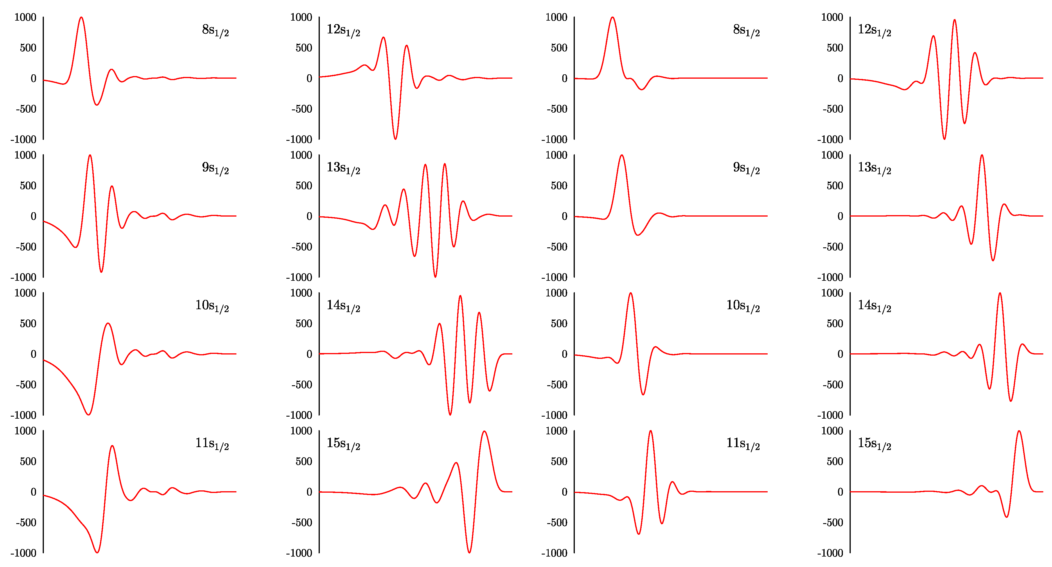
Virtual orbitals for the $s_{1/2}$ partial wave from the sets ${\mathsf{\Pi }}_{\pm }$ are shown in Figure 2. The left panel corresponds to the set ${\mathsf{\Pi }}_{+}$ and the right panel corresponds to the set ${\mathsf{\Pi }}_{-}$. One can see that virtual orbitals from these two sets are significantly different. The orbitals from the set ${\mathsf{\Pi }}_{-}$ are more localized and have a smaller number of nodes. Because of that, the operator U defined in Equation (6) in this case is numerically more stable. In particular, the deviations from orthogonality and normalization are smaller for the orbitals ${\psi }_p^{(-)}$ generated with the phase ${\alpha }^{(-)}$. The same applies for the partial waves $p_{1/2}$ and $p_{3/2}$. For the higher partial waves, the difference is less pronounced because of the smaller number of physical orbitals. We conclude that the basis set ${\mathsf{\Pi }}_{-}$ is preferable from the numerical point of view.

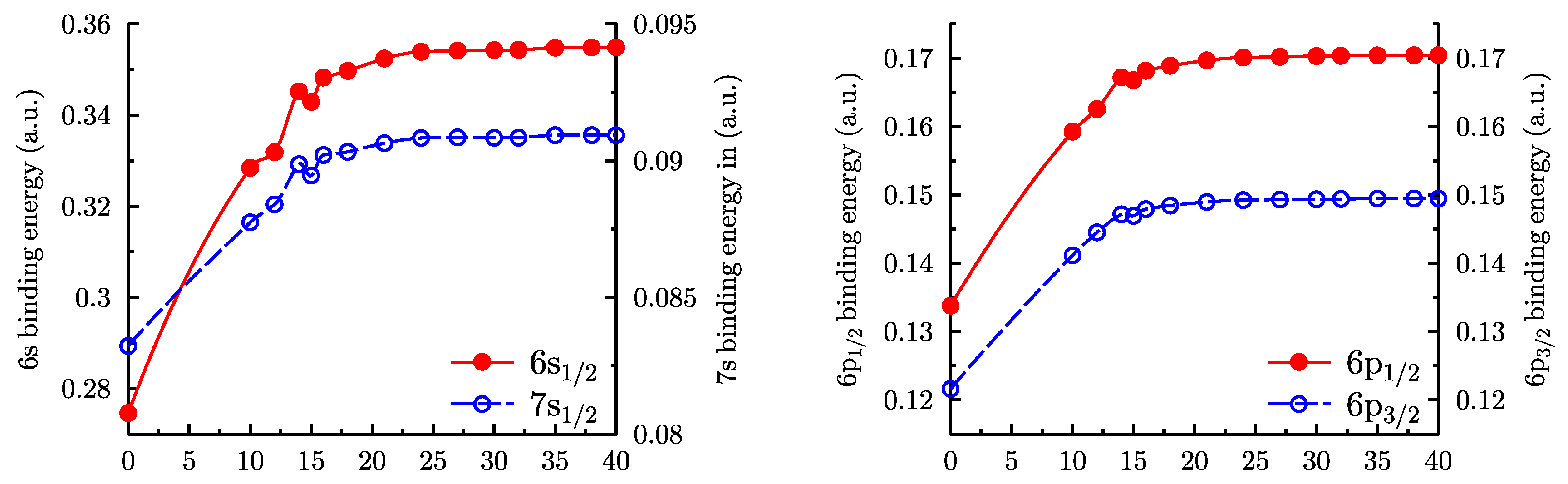
Now, we generate basis sets of different length and test convergence of the MBPT results for the binding energies of the lowest valence states of Au: $6s_{1/2}$, $6p_{1/2}$, $6p_{3/2}$, and $7s_{1/2}$. All basis sets include 11 partial waves up to $h_{9/2}$ and $h_{11/2}$. The number of B-splines of rank 5 is changed from 10 to 40. The last Dirac–Fock orbitals in the partial waves are $7s$, $6p$, $6d$, and $5f$. In the partial waves g and h, all orbitals are virtual.

The results of the second order MBPT calculation for the binding energies are shown in Figure 3. All second order expressions include summation over unoccupied orbitals [1]. Because of that, calculated energies depend on the number of splines in the basis set. For zero splines, all sums vanish, which corresponds to the Dirac–Fock approximation. We see that MBPT corrections are large, in particular, for the ground state $6s_{1/2}$, where they account for about 30% of the binding energy. For the number of splines above 18, the convergence is smooth and saturation is practically reached for 25 splines.

3.3. An Example of Au Atom: Hyperfine Structure

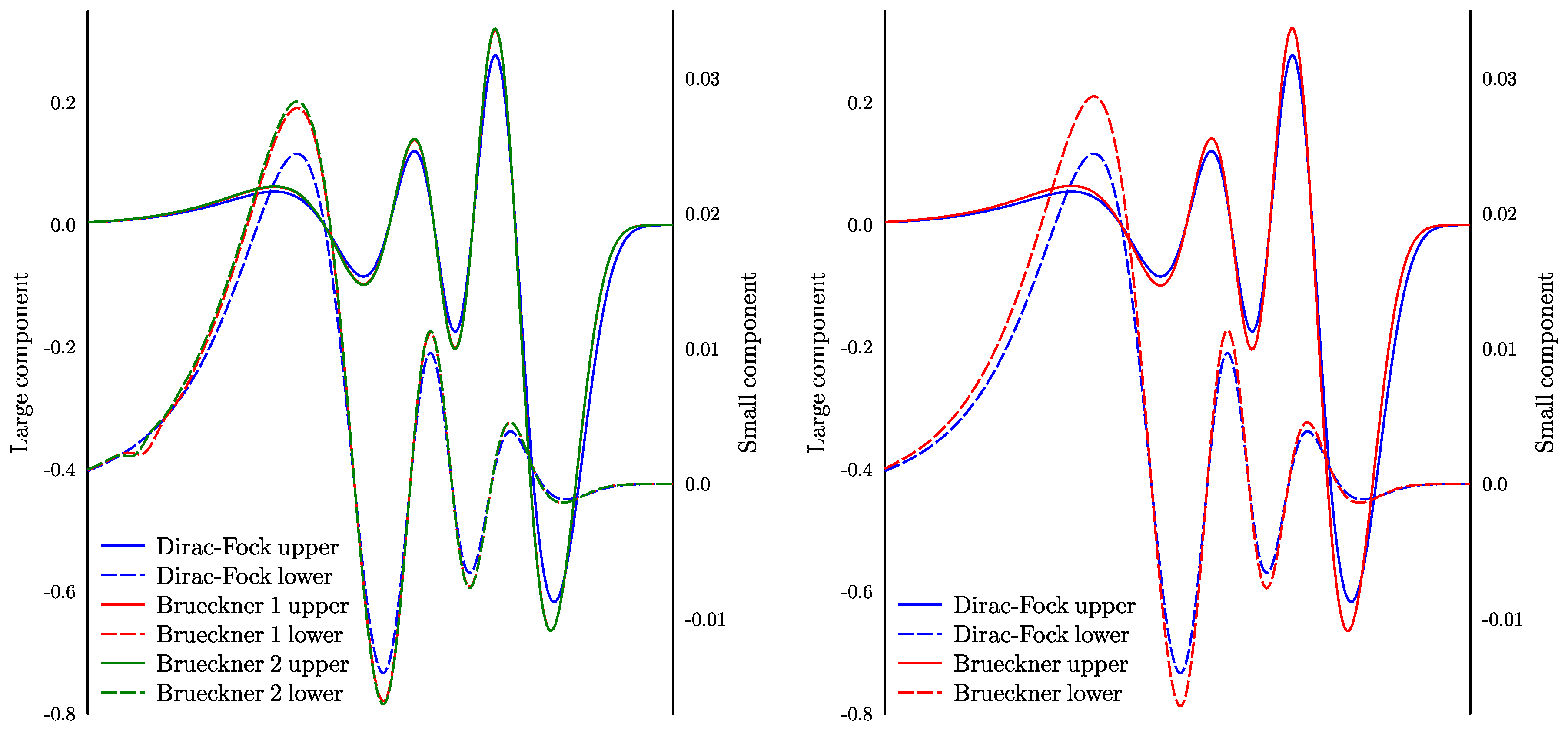
Let us consider magnetic hyperfine structure as an example of interaction which depends on the short distances. We do calculations for Au using the same MBPT wave functions as above and the random-phase approximation for the hyperfine operator. We neglect other corrections, such as ‘structural radiation’ [17] because they do not affect the convergence. We find that, in this case, the convergence is much slower and saturation is not reached even for 45 B-splines. In order to find the source of the problem, one can form Brueckner orbitals by diagonalizing one-electron MBPT corrections on the basis set of valence and virtual orbitals. The left panel of Figure 4 shows the $6s$ Brueckner orbital obtained using 35 and 45 B-splines. One can see that the resultant upper components are smooth everywhere and close to each other. However, the lower components at short distances have a dip. With a growing number of splines, the dip becomes smaller and closer to the origin but does not disappear (note that the radial variable is logarithmic). The matrix element of the hyperfine interaction depends on the product of the upper and lower components and, therefore, poorly converges.

We see that using only B-splines as virtual orbitals does not allow for a saturate basis set at short distances. We already mentioned above that, at short distances, it is difficult to accurately present a Dirac–Fock orbital as a linear combination of B-splines. Not surprisingly, the same applies to Brueckner orbitals. In order to improve convergence, one can add more physical orbitals with proper behavior near the origin. For example, one can use Dirac–Fock orbitals for other ionic states of the same atom. We added $6s$, $7s$, and $6p$ Dirac–Fock orbitals for the $V^{N-6}$ potential (half-filled $5d$-shell). After that, convergence for the hyperfine structure calculation dramatically improved and saturation was practically reached already for 24 B-splines of rank 4. Respective Brueckner orbitals are shown on the right panel of Figure 4. One can see that both large and small components are now smooth at all distances up to the origin. Convergence for the energies also improved but less impressively. Note that now our basis set includes three types of orbitals: the Dirac–Fock orbitals for the atom of interest, the orbitals for the ion stripped of several outermost electrons, and, finally, B-splines. We still use the same operator (6) to merge physical orbitals and B-splines together. This case demonstrates flexibility of the method, which allows for forming basis sets adjusted for different types of calculations. At present, we are finishing calculations of the hyperfine anomaly for Au. These calculations are done with the help of the basis sets described here.

4. Conclusions

Many numerical methods for atomic calculations require one-electron basis sets. It is important that these basis sets include physical orbitals, such as Dirac–Fock ones, for the occupied states. At the same time, using similar orbitals for virtual states is usually inefficient. Therefore, it is common to use B-splines, or other similar sets of orbitals. Here, we suggest a method to merge different subsets and form a joint orthonormal basis set. We use the unitary operator from Ref. [10] to substitute some of the orbitals from a chosen basis set with proper Dirac–Fock orbitals without losing the quality of the basis set, or running into problems with linear dependence between orbitals. We tested this method for Fr and Au using basis sets formed from B-splines of different ranks. The method proved to be sufficiently robust and we were able to reach convergence of the MBPT calculations for basis sets of moderate length even for sensitive properties, such as hyperfine structure.

References

- Dzuba, V.A.; Flambaum, V.V.; Kozlov, M.G. Combination of the many-body perturbation theory with the configuration-interaction method. Phys. Rev. A 1996, 54, 3948–3959. [Google Scholar] [CrossRef] [PubMed] [Green Version]
- Kozlov, M.G.; Porsev, S.G.; Safronova, M.S.; Tupitsyn, I.I. CI-MBPT: A package of programs for relativistic atomic calculations based on a method combining configuration interaction and many-body perturbation theory. Comput. Phys. Commun. 2015, 195, 199–213. [Google Scholar] [CrossRef] [Green Version]
- Bratsev, V.F.; Deyneka, G.B.; Tupitsyn, I.I. Application of Hartree-Fock method to calculation of relativistic atomic wave functions. Bull. Acad. Sci. USSR Phys. Ser. 1977, 41, 173. [Google Scholar]
- Savukov, I.M.; Johnson, W.R. Combined CI+MBPT calculations of energy levels and transition amplitudes in Be, Mg, Ca, and Sr. Phys. Rev. A 2002, 65, 042503. [Google Scholar] [CrossRef]
- Dzuba, V.A. VN−M approximation for atomic calculations. Phys. Rev. A 2005, 71, 032512. [Google Scholar] [CrossRef]
- Kahl, E.V.; Berengut, J.C. AMBiT: A program for high-precision relativistic atomic structure calculations. arXiv 2018, arXiv:1805.11265. [Google Scholar] [CrossRef]
- Kozlov, M.G. Precision calculations of atoms with few valence electrons. Int. J. Quant. Chem. 2004, 100, 336. [Google Scholar] [CrossRef]
- De Boor, C. A Practical Guide to Splines; Applied Mathematical Sciences; Springer: New York, NY, USA, 1978. [Google Scholar]
- Johnson, W.R.; Blundell, S.A.; Sapirstein, J. Finite basis sets for the Dirac equation constructed from B-splines. Phys. Rev. A 1988, 37, 307. [Google Scholar] [CrossRef] [PubMed]
- Abarenkov, I.V.; Tupitsyn, I.I. A new separable potential operator for representing a chemical bond and other applications. J. Chem. Phys. 2001, 115, 1650. [Google Scholar] [CrossRef]
- Tupitsyn, I.I.; Loginov, A.V. Use of sturmian expansions in calculations of the hyperfine structure of atomic spectra. Opt. Spectrosc. 2003, 94, 319–326. [Google Scholar] [CrossRef]
- Löwdin, P.O. On the Non-Orthogonality Problem Connected with the Use of Atomic Wave Functions in the Theory of Molecules and Crystals. J. Chem. Phys. 1950, 18, 365–375. [Google Scholar] [CrossRef]
- Aiken, J.G.; Erdos, J.A.; Goldstein, J.A. On Löwdin orthogonalization. Int. J. Quantum Chem. 1980, 18, 1101–1108. [Google Scholar] [CrossRef]
- Stanton, R.E.; Havriliak, S. Kinetic balance: A partial solution to the problem of variational safety in Dirac calculations. J. Chem. Phys. 1984, 81, 1910–1918. [Google Scholar] [CrossRef]
- Shabaev, V.M.; Tupitsyn, I.I.; Yerokhin, V.A.; Plunien, G.; Soff, G. Dual Kinetic Balance Approach to Basis-Set Expansions for the Dirac Equation. Phys. Rev. Lett. 2004, 93, 130405. [Google Scholar] [CrossRef] [PubMed] [Green Version]
- Girardeau, M.D. Completely Orthogonalized Plane Waves. J. Math. Phys. 1971, 12, 165–167. [Google Scholar] [CrossRef]
- Dzuba, V.A.; Flambaum, V.V.; Kozlov, M.G.; Porsev, S.G. Using effective operators in calculating the hyperfine structure of atoms. Sov. Phys. JETP 1998, 87, 885–890. [Google Scholar] [CrossRef]
Figure 1.
Examples of the same two component orthogonal B-spline for three partial waves with . The radial variable here and below is proportional to the logarithm of the radius.
Figure 2.
Upper components of the virtual orbitals for partial wave of Au atom generated from 15 orthogonal B-splines. Left (right) panel corresponds to the set (). See Equation (7) and the text for details.
Figure 3.
Binding energies for four lower levels of Au calculated within second order MBPT using B-spline basis sets of different length. The x-axis gives the number of virtual orbitals in a partial wave. Zero corresponds to the Dirac–Fock approximation.
Figure 4.
orbital for Au in Dirac–Fock and Brueckner approximations. Left panel: basis sets with 35 and 45 B-splines (labels 1 and 2, respectively); right panel: basis set of 24 B-splines with two additional Dirac–Fock orbitals in s wave.
© 2019 by the authors. Licensee MDPI, Basel, Switzerland. This article is an open access article distributed under the terms and conditions of the Creative Commons Attribution (CC BY) license (http://creativecommons.org/licenses/by/4.0/).
Share and Cite
MDPI and ACS Style
Kozlov, M.; Tupitsyn, I. Mixed Basis Sets for Atomic Calculations. Atoms 2019, 7, 92. https://0-doi-org.brum.beds.ac.uk/10.3390/atoms7030092
AMA Style
Kozlov M, Tupitsyn I. Mixed Basis Sets for Atomic Calculations. Atoms. 2019; 7(3):92. https://0-doi-org.brum.beds.ac.uk/10.3390/atoms7030092
Chicago/Turabian StyleKozlov, Mikhail, and Ilya Tupitsyn. 2019. "Mixed Basis Sets for Atomic Calculations" Atoms 7, no. 3: 92. https://0-doi-org.brum.beds.ac.uk/10.3390/atoms7030092
Note that from the first issue of 2016, this journal uses article numbers instead of page numbers. See further details here.