A Laboratory Astrophysics Problem: The Lifetime of Very Long-Lived Levels in Low-Charge Ions


AIRUB, Fakultät für Physik und Astronomie, Ruhr-Universität Bochum, D-44780 Bochum, Germany
Atoms 2020, 8(2), 21; https://0-doi-org.brum.beds.ac.uk/10.3390/atoms8020021
Submission received: 23 March 2020
/
Revised: 30 April 2020
/
Accepted: 2 May 2020
/
Published: 11 May 2020
(This article belongs to the Section Atomic, Molecular and Nuclear Spectroscopy and Collisions)
Abstract
:Emission lines of singly charged ions populate many astrophysical spectra. However, the interpretation of the line intensities (usually line ratios) often depends on the transition rates of the decays of very long-lived low-lying levels. For example, the line ratio of two electric-dipole forbidden transitions in the 3s3p ground configuration of singly ionized sulfur (ion S, spectrum S II) has been interpreted in terms of a density diagnostic for planetary nebulae, i.e., for densities in the order of 10 cm. The predicted lifetimes of the D levels are in the order of one hour. Modeling indicates that a 10% uncertainty of the lifetime determination in this case corresponds to a 50% uncertainty of the density diagnostic. The available theoretical lifetime predictions scatter by much more than 10%. Considerations about an experimental approach are presented with the goal of instigating a measurement of the actual level lifetimes.
1. Introduction
In the middle of the 19th century, astrophysical observations revealed several spectral lines that could initially not be reproduced in the laboratory. Such lines in regular solar spectra were thus assigned to a then hypothetical element Helium. Some lines observed only in the solar corona during solar eclipses were assigned to the hypothetical element ‘Coronium’, and the emission lines that dominated the spectra of planetary nebulae (objects misnamed because of the insufficient grasp of astrophysics at the time) were assumed to indicate yet another hypothetical element, ‘Nebulium’ [1,2]. Subsequently, helium was, after all, identified on Earth well before the end of the century. The progress of atomic physics permitted to classify most of the helium lines observed to electric-dipole (E1) allowed transitions in the electronic shells of the second-most abundant element in our universe. The apparent incompatibility of theory and observation for coronium and nebulium challenged some researchers to propose a variety of atoms of peculiar structure (for example, [3]), none of which was borne out by experiment. Coronium and nebulium also defied classification by the upcoming atomic structure theory as conceived based on Rutherford’s experiments, Bohr’s systematization, or Sommerfeld’s and Schrödinger’s nascent concepts of quantum mechanics. Eventually, Bowen recognized in the 1920s that the photon energies of the ‘nebulium’ lines matched fine structure intervals in various low-charge ions of ordinary elements such as nitrogen and oxygen (spectra N II, O II, O III) [4,5,6,7,8]. He explained the non-observation of these lines in the laboratory versus the observation in astrophysical objects such as planetary nebulae by the extremely low particle density of the latter which permitted radiative decays even of extremely low transition rates (Einstein A values) (electric-dipole ‘forbidden’ transitions, i.e., mostly magnetic dipole (M1), electric quadrupole (E2) transitions, magnetic quadrupole (M2) transitions, etc.) to take place before collisional quenching would happen. Correspondingly, Grotrian observed that the photon energies of several bright coronal lines came close to energy differences in the X-ray spectra of iron-group elements that had been obtained by Edlén [9]. He instigated Edlén to further increase the accuracy of his apparatus, and within a few years Edlén was able to practically prove that the ‘coronium’ lines originated from E1-forbidden transitions in the ground configurations of highly charged Ca, Fe, and Ni ions [10]. This insight revealed that the solar corona is much hotter than the underlying chromosphere and opened new avenues for trying to understand stars and their inner workings.
Concerning low or high charge states of ions in a plasma, the primary parameter of interest is temperature. In a plasma reasonably close to thermodynamical equilibrium, the velocity distributions of ions and electrons are described by Maxwellian functions. The fraction of electrons at the highest velocities (kinetic energies) is responsible for collisionally ionizing atoms and ions. The balance of ionization and recombination events eventually results in a charge state distribution that features high charge state ions only at high temperatures. Therefore, the appearance of high charge state ion spectra immediately serves as a rough temperature indicator. A second temperature gauge is available via level populations, because Boltzmann statistics includes the temperature as a parameter in the population law. One might observe line intensities as a function of principal quantum number n for this temperature effect, but then the spectral lines involved span a wide wavelength band over which the detection efficiency needs to be established in detail, which is very difficult. Moreover, the temperature effect there is superimposed on a dominant intensity variation which is due to atomic properties (such as wave functions with their scaling factor). Less direct, but more practical, is the study of line ratios in pairs of emission lines the upper levels of which are populated via different fine structure levels of the ground configuration. Here a major complication lies in the modeling of the line ratios by a collisional-radiative model that may imply hundreds or thousands of levels and tens of thousands of transitions. This technique carries a second complication; the ground configuration level populations depend not only on temperature, but also on density. At low density, an excited level can radiatively decay to the true ground level where the ion will then be available for the next collisional or radiative excitation event. At high density, in contrast, the next collision may take place before radiative de-excitation has occurred, and thus the line intensity pattern of subsequent emission may differ from the low-density situation. The actual level lifetime of the higher fine structure levels in relation to the time between collision matters; it determines the density at which the characteristic line ratios change from their low-density value to their high-density value.
In practice, any plasma, of course, has a temperature and a density. The signal observed on an individual emission line depends on the level population and the transition rate, both directly and in the form of the branch fraction, the ratio of a given transition rate to the total decay rate (the sum of all transition rates from a given level, and the inverse of the level lifetime). In the case of the S II line pair discussed below, one expects on statistical grounds a somewhat lower population of the fine structure level than that of the level. However, the decay rate of the level is about three times higher than that of the level. In the observed spectra the two spectral lines are of roughly equal intensity. Czyzak et al. [11] demonstrate how to exploit spectral modeling and how to interpret line ratios in terms of temperature and density and thus obtain an interesting tool for temperature and density diagnostics of remote plasmas.
Now why do some astrophysical objects feature ‘nebulium’ lines and others ‘coronium’ lines (only)? It is a matter of temperature and density. In the quiet solar corona (as a typical example) the electron density is of the order of = 10 cm, with flares and other active features reaching = 10 cm ([12,13,14] and many more; the solar corona features holes and many emissive structures, the electron density varies with time, location over the Sun, and distance from the Sun), at temperatures of 10 K (100 eV) and higher. In planetary nebulae the density is much lower, for example = 10 cm (see [11] and references therein), at temperatures of 10 K (1 eV) and lower. For the diagnostic studies of the solar corona, the levels of primary interest in suitable highly charged ions (say, Fe to Fe) feature lifetimes in the range of several milliseconds up to seconds and have been investigated in several types of ion traps (see [15,16,17,18,19,20] and discussion below). For the investigation of density effects in planetary nebulae, ions with level lifetimes longer by yet another 3 to 4 orders of magnitude are required. One prominent example is the O III lines (identified by Bowen [6], see above) near nm with an estimated upper level lifetime of about 40 s [21]. Other observations have long since revealed that the line pair “[SII]6700” (in a common astrophysical shorthand notation using wavelengths in Ångström), S 3s3p S – D, at wavelengths near 673 nm, should also be suitable for the determination of particle density in planetary nebulae. The line pair has been employed for density diagnostics using theoretical values for the level lifetimes (which are in the order of half an hour and an hour and a half, respectively), but the various predictions scatter by considerable amounts and thus indicate a notable degree of uncertainty. An experimental corroboration of the computational lifetime results is highly desirable, and much of this report deals with possible ways to achieve this. A first goal of laboratory work would be to determine the level lifetimes with an uncertainty of ±10%; for this uncertainty of the level lifetimes the modeling efforts indicate a 50% uncertainty of the density diagnostic [22]. More recent discussions highlight the importance and uncertainties of such work [23,24]. A higher accuracy than 10% would be welcome to test and help improve the various atomic structure computation packages and the modeling. The following presentation describes the case of S II in more detail and how an eventual experiment might proceed.
2. Atomic Structure
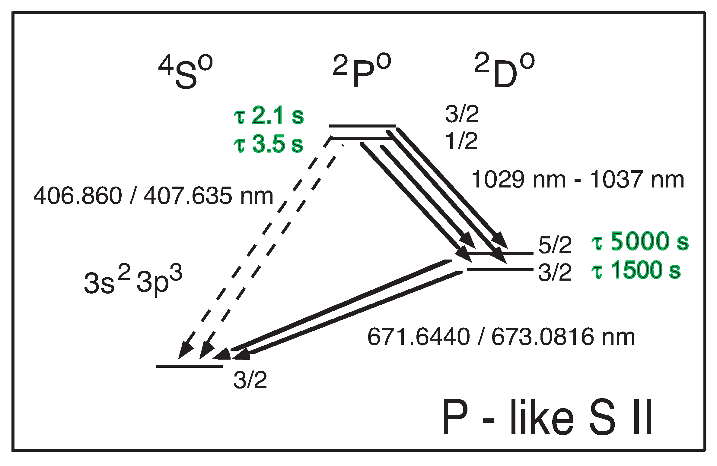
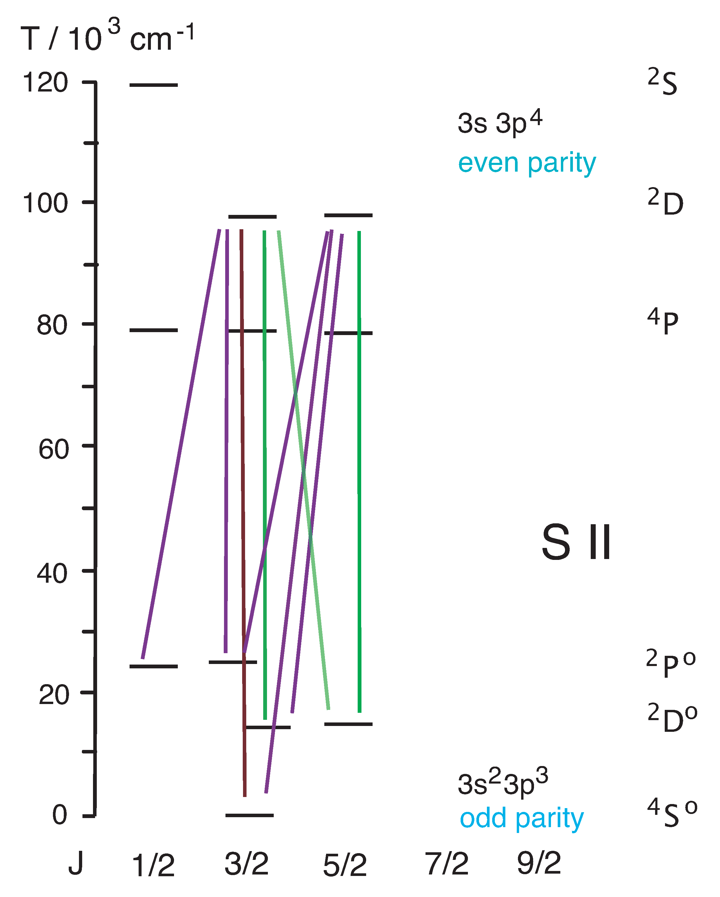
The structure of the 3s3p ground configuration of P-like ions (Figure 1) corresponds to that of the 2s2p ground configuration of N-like ions. In S II the transitions within the ground configuration fall into the blue, the red, and the infrared (IR). The transitions of principal interest for the density diagnostics of planetary nebulae are at wavelengths of 671.6440 nm and 673.0816 nm [21]. The levels depicted in the graphs are taken from the NIST ASD online data base [21]. It should be kept in mind that this data base represents a combination of (necessarily incomplete) observations and computations. Several plausible transitions are not listed in that data base. For example, there are displaced terms 3s3p (Figure 2), with five levels lying below the regular n = 4 levels and one lying among the n = 4 levels. All six of these displaced levels are listed in the NIST ASD online data base. However, apparently there are no transitions to lower levels given for the highest of these displaced levels, S. One must assume that not all S II transitions have been identified in laboratory spectra yet, nor are reliable computations available of all transition rates. However, most, if not all, of the S II transitions discussed below appear to be sufficiently well known.
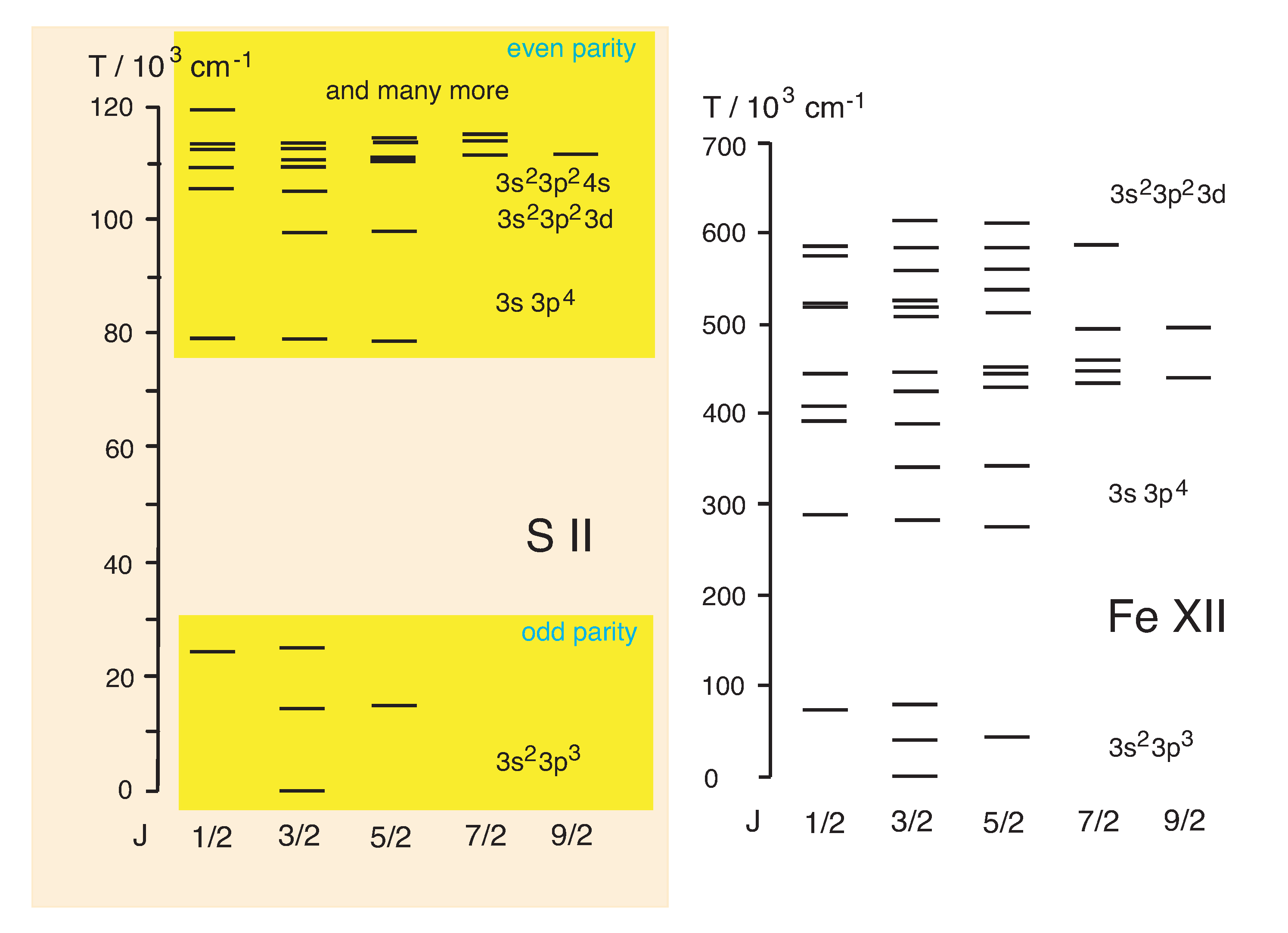
The various groups of levels scale differently with the nuclear charge Z. This is evident for the levels in Figure 3. The levels are not shown in that figure, because there are so many that some of them cannot be drawn separately at this scale.
3. Theoretical Work
Any theoretical treatment of P-like ions must cover all five levels of the ground configuration, because they all are of the same parity, and the upper level pairs each contain a level of the same J value as the ground level. The electric-dipole forbidden transition rates between these five levels are easy to obtain in principle, since in a single-configuration picture they depend only on a Racah algebra factor and the transition energy (to the third (fifth) power for M1 (E2) transitions, respectively). However, ab initio calculations of fine structure intervals (including the important level structure of the ground configuration in many-electron ions) are often not very accurate. This is suspected to be the main reason for the scatter of the various predictions of transition rates. Consequently, it is a wide-spread custom to use spectroscopic level data instead of the computed energies. On one hand, one hopes that this measure improves the validity of the computed results for the transition rates for practical purposes. On the other hand, the need for such a correction indicates a rather limited predictive power of the present-day application of atomic structure theory.
Czyzak and Krueger [25] were among the first to calculate the M1 and E2 transition rates in S II and several other ions. They also cite individual treatments by other authors (such as Pasternack and Garstang) and found (for S II) almost perfect agreement for the decay rate of the 3p D level on one hand and a variation by more than a factor of two for the 3p D level on the other. (Irritatingly, Garstang in a 1968 book contribution [26] claimed to cite the results of Czyzak and Krueger [25], but the data entries for these two levels of S II were incorrect by a factor of six in one case and by an order of magnitude in the other. At a Liège conference four years later, Garstang informed his audience about that mistake, as I happen to see noted in handwriting on a photocopy (of unrecorded provenance) of that book contribution.) Later results [21,22,27,28,29,30,31,32,33,34,35] shifted from the early ones by a significant amount, but they also scattered quite notably (Table 1, Figure 4). The study by Mendoza and Zeippen [27] has been claimed in later publications as the first one with reliable results. Froese Fischer and Godefroid [31] have “updated” several the earlier results for the 3p D level lifetimes by a correction of the computed transition energies to match the experimentally known ones, and the data in the table represent these updated numbers as far as they are available.
The computations have employed a variety of programs and approaches, including relativity even for such near-neutral ions. Owing to the growing availability of computing power, one may assume that overall the accuracy increases over time, but the actual accuracy apparently has not been quantified by any of the authors of the theoretical studies. In such exploratory computational investigations it should not come as a surprise that later work does not necessarily improve on all aspects of earlier studies. For example, Keenan et al. [22] concede that the intrinsic accuracy of some of their operators may be insufficient, because some series expansions did not extend far enough. In this case, they combine their own E2 transition rates with the M1 transition rates obtained by Mendoza and Zeippen almost a decade earlier [27]. The study by Fritzsche et al. [32] comprises a useful literature search and introduces fully relativistic computations. Froese Fischer et al. [31,34] can boast of a particularly extensive experience in the field of such computations. It is not surprising to see the latest four studies [21,33,34,35] producing results that lie close to the visual average of all available computational results. However, the results for the two S II levels of primary interest have developed differently over time (see Figure 4), and a quantification of the accuracy is still lacking.
The prospective measurement of the 3s3p D level lifetimes of S II poses an extreme challenge. It may be sensible to test a prospective experimental set-up for this task on the less extreme case of the 3s3p P levels of the same ion. Here the level lifetimes have been calculated to lie in the range of a couple of seconds (Table 2), which should be much easier to measure than the hour-range lifetimes of the 3s3p D levels. Figure 5 reveals that the scatter of the predictions is sizeable in this case, too.
4. Previous Experiments on Other Ions
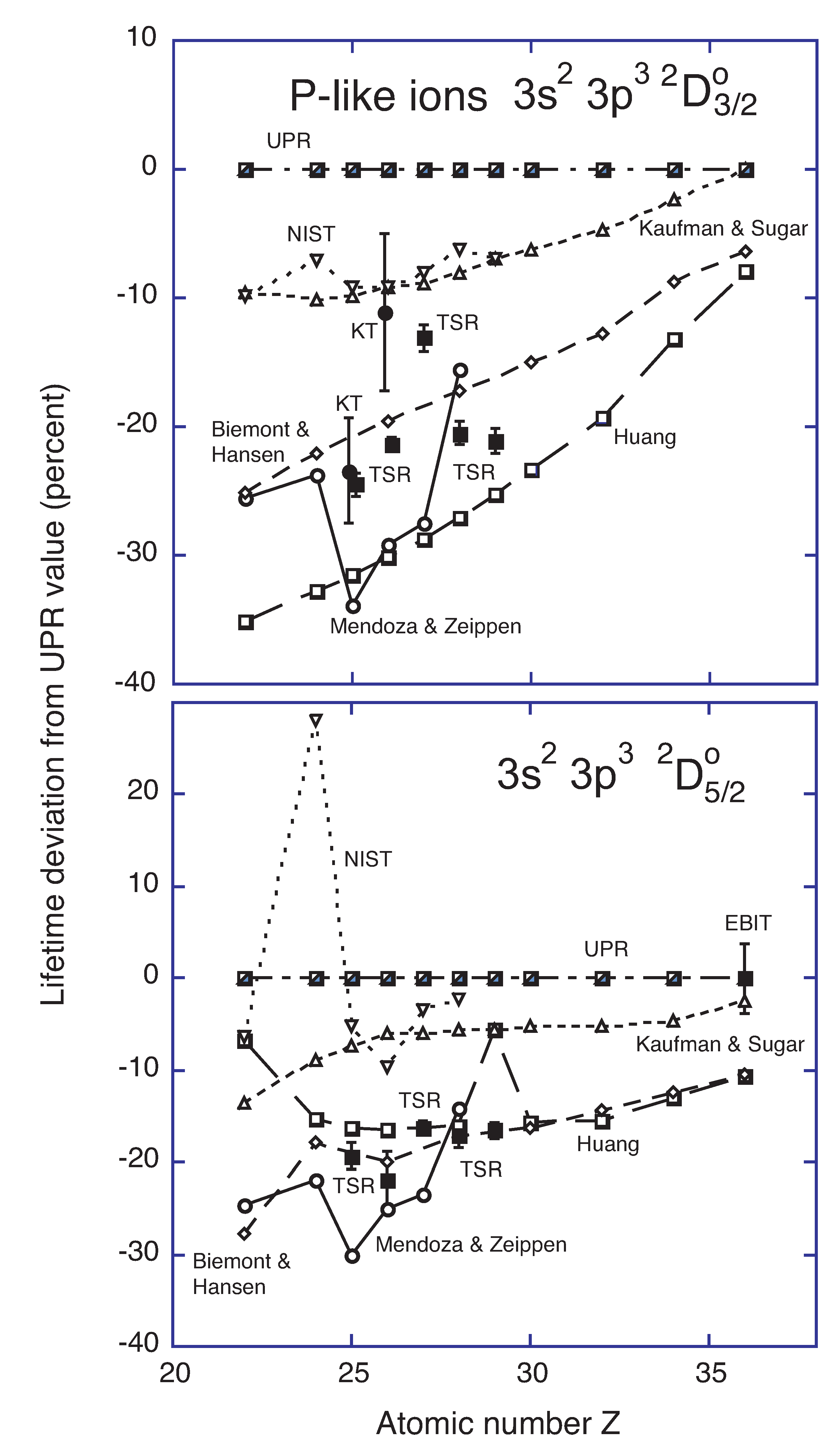
There are no experimental data on the two level lifetimes of primary interest in S II yet. The E1-forbidden transition rates scale steeply with the transition energy ( or for M1 and E2 transitions, respectively), and that energy interval in turn scales steeply with the nuclear charge Z (fine structure intervals grow with ). The level lifetime drops correspondingly steeply with increasing Z, and measurements with established techniques have been feasible so far only for a range of multiply charged ions. The lowest-Z measurements on ions of the P I isoelectronic sequence have been reported for (Mn), and the highest-Z ones for (Kr). Figure 6 shows comparisons of these lifetime data [15,16,17,18,19] obtained by work with a variety of ion traps (electrostatic (Kingdon) trap, heavy-ion storage ring, electron beam ion trap) with various predictions. To accommodate all experimental and computational results on a common footing and practical scale, they are displayed by their (relative) difference from a computed reference set. Since not all computations using a given approach [21,27,28,29,30] had been applied to all elements in this range, computations employing a multi-reference Møller–Plesset code were executed by Diaz, Ishikawa, and Santana at the University of Puerto Rico (UPR) [18] to provide such a reference. Strikingly, for high values of the nuclear charge in this sample, , all computational predictions agree with each other to within about 10%, whereas at the low-Z end of the display, near , the bandwidth of the predictions spans about 30%. This trend fits to the even larger spread of predictions for discussed in the preceding section. Moreover, there is no set of predictions that agrees fully with all experimental results. Figure 6 suggests that the Co XIII 3s3p D experimental data point may be an outlier. Among the available computations, the work of Biémont and Hansen [29] comes closest to the majority of the experimental results. One might expect that the results of computations should show similar smooth trends. However, the results presented by Mendoza and Zeippen [27] and some of Huang’s results [28] show a ragged difference curve in comparison with the other computations. Also, a data entry for (Cr) in the NIST tables may be clerically faulty. Several of the predictions may by now be considered obsolete, but the situation remains less clear-cut than one would hope for.
Evidently, most computations converge better for high ion charges where the central Coulomb field plays a dominant role, and the predictions come closer to the experiment in this high-Z range. However, for our astrophysical problem, we seek reliable results at low Z. Most computations are not tailored for this range and do not converge well for near-neutral ions. Thus, we find theory to be of limited reliability as a source of guidance for singly charged ions such as S, although this is the very range of low ion charge that is of dominant importance in much of astrophysics—and in our terrestrial environment, too.
A level lifetime of about ten years has been inferred from the excitation characteristics of a high-angular momentum level of a trapped singly charged ion of a heavy isotope Yb [36], which apparently is the longest atomic level lifetime ‘measured’ so far. The estimate includes a determination of the line width of an electric octupole (E3) transition, the line width being inversely related to the level lifetime. Correspondingly, the line widths of the ground state transitions S II 3s3p S–D are expected to be in the order of 0.1 mHz and would have to be measured to better than 10% of this value. This technique is complementary to, but very different from, the experimental schemes discussed above and below which aim at observing the time history of a level population. In multi-electron systems such as the Yb ion there are many levels that are in reach by laser above the metastable level of interest. In favorable cases, the population of the latter can be probed by exciting the ion to another level from which the decays lead back to the level of interest, and thus the long-lived level population is not lost. Consequently, the same ion can be interrogated several times while being stored for long time intervals. Because of the simpler structure of atoms with fewer electrons, this feature is not available in the much lighter ions discussed below.
The Heidelberg test storage ring TSR [37] has served for measurements of long-lived levels in many ion species (see examples above). Most of these were moderately to highly charged, and the lifetimes (in the range from milliseconds to several seconds) were long only in comparison to the lifetimes of levels that predominantly decay by E1-allowed transitions [20]. In terms of lifetime measurements of very long-lived levels, the TSR heavy-ion storage ring has provided a result of about 52 s in a dielectronic recombination (DR) measurement on the long-lived 1s2s S level in Li ions [38]. This is not far from the lifetime of the aforementioned O III 2s2p D level (a representative prediction is 41 s [30]) the decay of which (by M1 and E2 transitions) to the O III 2s2p P ground term and in particular to the P level, gives rise to the astrophysically famous line near 500.7 nm, one of the ‘nebulium’ lines that Bowen identified correctly and that still serves as a diagnostic reference in many astrophysical spectra. However, the TSR heavy-ion storage ring is no longer available for such experiments; it has been closed down and is undergoing refurbishment for new uses in isotope studies at CERN/ISOLDE.
Atomic level lifetimes of hundreds of milliseconds up to the range of minutes have been measured in the FERRUM project at Stockholm [39]. The singly charged ions (including some in metastable levels) were produced in an electrical discharge ion source. After extraction and mass selection, a beam of the wanted ion species was stored in the CryRING heavy-ion storage ring. At some time after injection into the ring, an intense laser pulse would excite the remaining excited ions to higher-lying levels from which they could promptly decay (via E1 transitions) to the ground state. The corresponding light signal was assumed to represent the number of surviving excited ions, and a decay curve was built up point by point with a single laser-quenching event per cycle. Various multi-second lifetimes were measured by this technique (for example, [39,40,41]). Among the particularly long-lived levels studied was a level in Ti II with a 28 s mean life [42]. This, again, is a result in the same time range as the expected O III lifetime of astrophysical interest mentioned above. The CryRING apparatus at Stockholm has since been decommissioned and is now serving new uses, mostly on highly charged ions, under the name CRYRING@ESR at the FLAIR facility of the Darmstadt (Germany) heavy-ion research center [43].
In a wider sense of ‘experiment’, the relative intensities of certain lines in astrophysical sources have been interpreted in terms of transition rates and thus of level lifetimes, such as line ratios of magnetic quadrupole (M2) and hyperfine-induced transitions in four-electron ions. For example, in the Be-like ion N, the N IV 2s2p P level decays by a hyperfine-induced transition to the 2s S ground state. Interpreting UV spectra of a planetary nebula, obtained by the Hubble space telescope, and applying spectral modeling, Brage et al. [44] see the observed line ratio as compatible with a computed 40 min level lifetime (and an uncertainty of 1/3) of the upper level. A direct measurement of the transition rate would be highly appreciated by the community.
5. Considerations on S II Measurements
The O ion (N-like spectrum O II) is structurally closely related to S (P-like spectrum S II). The 2s 2p S – D transitions have wavelengths of 372.6032 and 372.8815 nm, respectively [21]. Apparently, these wavelengths have been measured accurately in astrophysical observations. The transition rates have not yet been measured, and the predicted level lifetimes are in the order of 5630 s and 32,700 s, respectively [21]. This longevity and the high astrophysical abundance of oxygen render O II a very interesting probe for even lower densities than have been discussed for S II. However, the measurement of such lifetimes by the techniques discussed below for S II would be even more demanding. Although the measurement would be of considerable interest, it probably will have to wait until after the eventual S II D level lifetime measurement.
The aforementioned O ion (spectrum O III) and its 500.7 nm line (decay of the 2s2p D level with a predicted lifetime of about 41 s) have been studied theoretically since decades, but there is no lifetime measurement result available yet. The rather similar case of the S ion (spectrum S III) (decay of the 3s3p D level with a predicted lifetime of about 15 s [21]) entails the problem of dominant decay branches in the near IR (at wavelengths of 953 nm and 907 nm, respectively), for which present detectors feature an intrinsically high noise rate.
These examples of doubly charged ions will not be discussed any further here, because in terms of the necessary ion storage times they seem to be tractable problems that might be taken care of with relatively little effort at one of the (few) heavy-ion storage rings that still exist. However, one must keep in mind that it is not sufficient to observe some stored ions for the duration of one or two atomic level lifetimes. There typically are ion losses to correct for; the inverse of the loss rate may be seen as an ion-beam storage lifetime. In order to remain a manageable correction, this entity must be considerably longer than the expected atomic level lifetime. This is harder to achieve for ions with many electrons than for bare ions, because both electron capture and loss are more likely to happen with ions that feature bound electrons that are available for the energy and momentum matching and that in this way contribute significantly to the ion loss cross section.
Obviously, these collisional electron capture loss processes may be problematic with an ion carrying as many as 15 electrons such as S (spectrum S II). Moreover, the cross sections are largest at some relatively low collision velocity. Consequently, heavy-ion storage rings provide much shorter ion storage times at low ion-beam energies (below, say, 100 keV) than at high ones (say, many MeV). This feature immediately suggests the use of small ion traps, which are much cheaper to build and operate than a storage ring, and of cryogenic techniques to help with achieving the required excellent vacuum (see below). At ion kinetic energies in the order of, say, less than 10 eV, particle loss by ionization should be a minor problem.
5.1. Laboratory Work
Any laboratory study of ions with level lifetimes on the scale of an hour is demanding the utmost in terms of ultrahigh vacuum.
The thermal velocity of N molecules in ambient air (as an example of a mass close to that of S ions) is in the order of 300 m/s. Excite the ion here and now, then look for it an hour later: in free space it will be thousands of km away. Consequently, any laboratory research on the long-lived levels needs an ion trap, most simply a radiofrequency (Paul) trap, or a Penning trap (if a superconducting magnet is available).
For the study of S ions, gas injection into such a trap may use SF or HS, for example. SF has been used for decades as an “inert” insulator gas in electrical installations such as high-voltage transformers and particle accelerators; recently it has been banned, because the molecule contains fluorine (and thus any spillage threatens to contribute to the ozone hole in the upper atmosphere). HS, in contrast, is outright poisonous. However, only minute quantities are required; a density of 10 cm (as in planetary nebulae) corresponds to a pressure of about 10 mbar. Indeed, the laboratory vacuum must be about as good as the ambient pressure in planetary nebulae, and preferably even better. A major challenge arises from the fact that in astrophysical observations the light source may be observed with a large optical depth, so that many ions may contribute to the signal. In contrast, in the laboratory the observation may have to deal with just a few ions or even a single one inside a small volume. Such a good vacuum is achievable in the laboratory, but (expensive) ultrahigh vacuum (UHV) equipment is essential. An important parameter in the provision of extremely low gas pressures is the temperature. Cryogenic devices in various laboratories, ranging from Penning traps, radiofrequency ion traps [45], and electron beam ion traps [46,47], to the Heidelberg cryogenic storage ring CSR [48], have demonstrated the necessary techniques.
5.1.1. How to Excite the Ions in the Trap
(a) Single-photon direct excitation from the 3s 3p S ground level to the 3s 3p D levels using light with a wavelength near 670 nm is not very effective. The transition is an E1-forbidden M1 transition; there is no change of parity as would be necessary for E1 transitions. It might be more efficient to consider instead a two-photon transition induced by a laser operating at 1340 nm (schematic in Figure 7). Moreover, a larger sample of ions would be reached by the virtue of Doppler-free two-photon excitation compared to narrowband single-photon excitation. IR laser light of wavelength 1340 nm falls into in a wavelength range in which numerous lasers have been operated (not so far from the so-called telecoms window near 1500 nm that is used in communications via glass fibers). Moreover, this bright laser light would be far from the detection wavelength of a single-photon decay. A small sample of ions, ideally a single ion in the trap, would be of interest in a measurement that aims at measuring the line widths of the 3s 3p S–D transitions. Such a Lorentzian line profile is the Fourier transform of the exponential decay function of the upper level, and the line width corresponds to the inverse of the upper level lifetime. However, collisions would shorten the upper level lifetime and thus broaden the line profile by convoluting it with a Gaussian (the result of the convolution is a Voigt profile). A line width determination that does not account for the collision-induced broadening yields no more than a lower limit of the true level lifetime result. Measuring such a line width in trapping cycles of mere minutes might seem more manageable than a lifetime measurement that requires hour-long ion storage times. However, the collisional broadening is similarly adverse for atomic line width determinations in the order of 10 Hz as are collisions that shorten the required 10 s ion storage periods. Both approaches require extremely clean vacuum vessels and excellent UHV conditions.
(b) An alternative is the indirect excitation from the 3s 3p S ground level via an E1 intercombination (spin-changing) transition (of moderately low transition rate) to the 3s 3p D levels (induced by laser light of a wavelength near 102.1 nm) with a subsequent spontaneous E1 spin-conserving radiative decay to 3s 3p D (Schematic in Figure 8). The provision of vacuum ultraviolet (VUV) or extreme ultraviolet (EUV) laser light in the wavelength range 100 to 150 nm may presently be achieved by high-harmonics production in non-linear media or alternatively by synchrotron radiation. This option does not require any IR laser, but needs intense VUV/EUV light at two wavelengths, for excitation and probing (see below).
(c) Another alternative is an E1 spin-conserving (“easy”) excitation from the 3s 3p S ground level to the 3s 3p P levels (which have a lifetime of about 20 ns); laser light with a wavelength near 125 nm is required. The subsequent spontaneous E1 intercombination radiative decay ( 155 nm) (among others) to the 3s 3p D levels, unfortunately, features an unfavorable branching fraction (schematic in Figure 9).
Option (a) with two-photon excitation appears the most attractive one to this researcher.
5.1.2. How to Sense the Level Population as a Function of Time (Optical Detection Schemes)
Simply waiting for photons from the radiative decays of the excited ground configuration levels of interest is very inefficient, since the noise rate of any known detector for 670 nm light is many orders of magnitude higher than the expected signal rate. Moreover, any practical light collection system would cover a solid angle of detection that amounts to no more than only a small fraction of 4. Various laser experiments have exploited the principle of laser quenching instead: The population of an excited level is probed by excitation via an E1-allowed transition to another, higher-lying level, and the subsequent (and fast) decay of the latter is observed with a good signal-to-noise ratio. In the case of the 3s 3p D levels of present interest one can choose from several paths. All these options test the level population destructively.
(a) E1-forbidden transitions 3s 3p D levels (with wavelengths near 1030 nm, see Figure 1) to the 3s 3p P levels are of little interest, because the latter decay to ground, but only slowly (as mentioned above; the multi-second lifetime measurement of these levels needs an experiment of its own). However, the transition wavelength of the dominant decay branch to the ground level lies in the blue—which is reasonably good for a low-noise photomultiplier tube (PMT) as the detector.
(b) E1 transitions to the 3s 3p D levels (Figure 10) have wavelengths near 120 nm, which is not particularly good for lasers, but there are numerous lasers and synchrotrons available in specialized laboratories all over the world that yield such light. The subsequent intercombination decays to ground (at 82.3 nm) have low rates, whereas the decay rates to the 3s 3p P levels (at 136 nm) and the 3p D levels (at 120 nm, back to the level of origin) are reasonably high. The suppression of the stray light from the bright VUV excitation light could be effected with a LiF or MgF filter (transparent above 110 nm and 120 nm, respectively, working as an edge filter) in front of a solar blind VUV detector.
(c) E1 transitions to the 3s 3p 3d F levels have wavelengths near 100 nm (shorter than H I Ly): a severe problem for lasers. From there, the ions would decay to levels of the ground configuration.
(d) Two-photon transitions to the 3s 3p 4p levels need about 150 to 190 nm photons each, which is not easy to provide for lasers. The observation of subsequent 4s-4p transitions requires IR detection at wavelengths of 1000 nm and longer—which is definitely unfavorable.
Option (b) might be the most promising one among the optical techniques. Instead of high-harmonics generation of visible laser light to reach the 8 to 12 eV photon energy needed for the population probe, an alternative might be offered by synchrotron radiation, especially as it is tunable in wavelength. Thus, there are two narrowband steps in the experiment (direct or indirect excitation from the ground level to the levels of interest, and excitation from one of the levels of interest to a 3s 3p level; the subsequent decay can be observed in the vacuum UV with little wavelength discrimination.
5.1.3. How to Sense the Level Population as a Function of Time (Non-Optical Detection Scheme)
A completely different detection scheme is available from mass spectrometry of single ions in a Penning trap. Ground state and excited ions differ by the excitation energy, which in S ions amounts to about 2 eV compared to the total mass of a mass-32 ion of about 32 GeV/c. Thus, a ‘weighing’ process with a relative resolution of should be able to discriminate between the ground state and the excited state S ion. This goal has, in fact, recently been achieved on stored Re ions in a cryogenic Penning trap, and a very long-lived metastable level has been detected this way [49]. The levels of interest in S ions are the only long-lived ones within some 10 eV of the ground level; practically all levels beyond 10 eV are shorter lived by many orders of magnitude. In the present context it is not necessary to accurately determine the level spacing by mass spectrometry. A few dozen seconds after the excitation of a single trapped ion (by laser, as described above), only the two long-lived levels 3s 3p D will be populated. When using two-photon spectroscopy for the initial excitation, it should be feasible to excite either one of the two levels at will. The two D levels are too closely spaced to detect their mass difference by present-day mass spectrometry. The frequency measurement involved in the mass spectrometry process must be only sufficiently sensitive to detect the change in frequency resonance that tells of the difference between ground state and the lowest excited levels. The time after excitation that the ion remains excited contributes a data point to a decay curve; when the ion de-excites, the resonance frequency shifts accordingly, and the excitation system can be triggered to begin a new measurement cycle. It should be straightforward to disentangle the joint decay curve in terms of the two individual contributions.
Obtaining a narrow resonance curve requires sufficient measurement time. With the many-minute level lifetimes in the S ion this atomic system seems compatible with the measurement process. This version of the experiment on S ions requires a cryogenic precision Penning trap and a laser for two-photon excitation, but it would do without EUV/XUV excitation by powerful photon sources, and thus avoid the solid-angle limitation of most optical detection schemes. There is only a single optical window (for example, a glass fiber feedthrough) required to transport the IR radiation into the trap; two-photon laser spectroscopy usually works with a retro-reflector to provide the second laser beam. This light beam can be injected close to the axis of a Penning trap and thus without significant mechanical changes to the given cylindrical Penning trap arrangement.
Of course one must not overlook that a precision Penning trap experiment has the same extraordinary vacuum requirements (greatly helped by work at cryogenic temperatures) as the other experiments discussed above. The precision mass spectroscopy measurement (here used as a level population monitor) is intricate and demanding as well, even as no absolute mass measurement is involved. However, with several laboratories presently pursuing such mass spectrometry for fundamental physics research, it might be relatively simple to add a laser excitation system to such a working set-up.
6. Conclusions
There are very many astrophysics and atomic physics problems out there that have not been solved, and many of these may never be solved by experiment. Therefore, why care about this one? Actually, a large fraction of astrophysical spectra is populated by transitions in singly charged ions, and the signal carries information about dilute plasmas across the universe. While it is easy to produce spectra of such ions in the laboratory, it is not trivial to actually see in the laboratory the decays that matter under very low-density environmental conditions, and to obtain quantitative information on transition rates. In this sense, the proposed experiment on S II is a prototype experiment for several cases of astrophysical interest (mentioned above), mostly in the context of planetary nebulae.
It is also a very challenging (difficult and expensive) problem for experimenters, requiring a combination of ion trapping, UHV techniques, IR and VUV/EUV lasers, or access to a beam line at a sufficiently brilliant synchrotron, or high-level experience with high-resolution mass spectrometry at the leading edge of research. It seems easier for researchers with experience in the field of VUV/EUV lasers to gain sufficient expertise with the basics of how to trap ions rather than the other way round. Starting from high-resolution mass spectrometry using a Penning trap, it even appears to be relatively straightforward to add a two-photon laser system with a single glass fiber light guide for the excitation of a sample ion.
Considering the aforementioned case of N IV with line ratios that include M2 and hyperfine-induced decay channels (see [44]), the level lifetime is in the same range as discussed above for S II, the ion charge is notably higher, but the required resolution of a mass spectroscopic experiment is less stringent than for S II. In the case of N IV, the level of interest lies about 8 eV above ground, while the atomic mass is in the order of 14 GeV. Consequently, the relative mass resolution required amounts to . This is easier to achieve than the requirement for S, but the higher charge state and the shorter wavelength of the exciting photons cause other problems. None of this is easy.
7. Author Note
The S II lifetime problem has resurfaced at a 2019 astrophysics conference, somebody wondering why this case has not yet been solved. For the time being the problem is a challenge to atomic structure computationalists, as is evident from the scatter of the presently available level lifetime predictions. In the longer run, an experimental answer to the challenge would be preferable.
As a retired atomic physicist I am enjoying the hospitality of an astrophysics institute. I have worked with various ion traps, but not with lasers for excitation etc. Therefore, it is quite possible that to a laser expert some of my ideas may seem mistaken. These notes are meant to help somebody (not yet identified) who may be interested in such a project. Hints for improvement of these notes are welcome.
Funding
This research received no external funding.
Acknowledgments
The hospitality of the astronomy chair of AIRUB (R.-J. Dettmar) is greatly appreciated.
Conflicts of Interest
The authors declare no conflicts of interest.
References
- Huggins, W.; Miller, W.A. On the Spectra of some of the Nebulae. Trans. R. Soc. Lond. 1864, 154, 437–444. [Google Scholar] [CrossRef]
- Huggins, M.L. Teach me how to name the – light. Astrophys. J. 1898, 8, 54. [Google Scholar] [CrossRef]
- Nicholson, J.W. A structural theory of the chemical elements. Philos. Mag. 1911, 22, 864–889. [Google Scholar] [CrossRef]
- Bowen, I.S. The Origin of the Nebulium Spectrum. Nature 1927, 120, 473. [Google Scholar] [CrossRef]
- Bowen, I.S. The origin of the chief nebular lines. Proc. Astron. Soc. Pac. 1927, 39, 295B. [Google Scholar] [CrossRef]
- Bowen, I.S. The origin of the nebular lines and the structure of the planetary nebulae. Astroph. J. 1928, 67, 1B–15B. [Google Scholar] [CrossRef]
- Bowen, I.S. The spectrum and composition of the gaseous nebulae. Astroph. J. 1935, 81, 1B–16B. [Google Scholar] [CrossRef]
- Bowen, I.S. Forbidden lines. Rev. Mod. Phys. 1936, 8, 55–81. [Google Scholar] [CrossRef]
- Grotrian, W. Zur Frage der Deutung der Linien im Spektrum der Sonnenkorona. Naturwissenschaften 1939, 27, 214. [Google Scholar] [CrossRef]
- Edlén, B. Die Deutung der Emissionslinien im Spektrum der Sonnenkorona. Z. Astrophys. 1942, 22, 30E. [Google Scholar]
- Czyzak, S.J.; Keyes, C.D.; Aller, L.H. Atomic structure calculations and nebular diagnostics. Astroph. J. Suppl. 1986, 61, 159–175. [Google Scholar] [CrossRef]
- Mercier, C.; Chambe, G. Electron density and temperature in the solar corona from multifrequency radio imaging. Astron. Astroph. 2015, 583, A101. [Google Scholar] [CrossRef]
- Hayes, A.P.; Vourlidas, A.; Howard, R.A. Deriving the electron density of the solar corona from the inversion of total brightness measurements. Astrophys. J. 2001, 548, 1081–1086. [Google Scholar] [CrossRef]
- Aschwanden, M.J.; Benz, A.O. Electron densities in solar flare loops, chromospheric evaporation upflows, and acceleration sites. Astrophys. J. 1997, 480, 825–839. [Google Scholar] [CrossRef]
- Moehs, D.P.; Church, D.A. Measured lifetimes of metastable levels of Mn X, Mn XI, Mn XII, and Mn XIII ions. Phys. Rev. A 1999, 59, 1884–1889. [Google Scholar] [CrossRef] [Green Version]
- Moehs, D.P.; Bhatti, M.I.; Church, D.A. Measurements and calculations of metastable level lifetimes in Fe X, Fe XI, Fe XII, Fe XIII, and Fe XIV. Phys. Rev. A 2001, 63, 032515. [Google Scholar] [CrossRef] [Green Version]
- Träbert, E.; Hoffmann, J.; Krantz, C.; Wolf, A.; Ishikawa, Y.; Santana, J.A. Atomic lifetime measurements on forbidden transitions of Al-, Si-, P- and S-like ions at a heavy-ion storage ring. J. Phys. B At. Mol. Opt. Phys. 2009, 42, 025002. [Google Scholar] [CrossRef]
- Träbert, E.; Grieser, M.; Krantz, C.; Repnow, R.; Wolf, A.; Diaz, F.J.; Ishikawa, Y.; Santana, J.A. Isoelectronic trends of the E1-forbidden decay rates of Al-, Si-, P-, and S-like ions of Cl, Ti, Mn, Cu, and Ge. J. Phys. B At. Mol. Opt. Phys. 2012, 45, 215003. [Google Scholar] [CrossRef]
- Träbert, E.; Beiersdorfer, P.; Brown, G.V.; Chen, H.; Thorn, D.B.; Biémont, E. Experimental M1 transition rates in highly charged Kr ions. Phys. Rev. A 2001, 64, 042511. [Google Scholar] [CrossRef]
- Träbert, E. E1-forbidden transition rates in ions of astrophysical interest. Phys. Scr. 2014, 89, 114003. [Google Scholar] [CrossRef]
- Kramida, A.; Ralchenko, Y.; Reader, J.; NIST ASD Team. NIST Atomic Spectra Database (ver. 5.7.1); National Institute of Standards and Technology: Gaithersburg, MD, USA, 2019. Available online: https://physics.nist.gov/asd (accessed on 26 January 2020).
- Keenan, F.P.; Hibbert, A.; Ojha, P.C.; Conlon, E.S. Einstein A-coefficients for transitions among the 3s23p3 states of S II. Phys. Scr. 1993, 48, 129–130. [Google Scholar] [CrossRef]
- Mendoza, C.; Bautista, M.A. Testing the existence of non-Maxwellian electron distributions in H II regions after assessing atomic data accuracy. Astrophys. J. 2014, 785, 91. [Google Scholar] [CrossRef] [Green Version]
- Juan de Dios, L.; Rodríguez, M. The impact of atomic data selection on nebular abundance determinations. Mon. Not. R. astron. Soc. 2017, 469, 1036–1053. [Google Scholar] [CrossRef] [Green Version]
- Czyzak, S.J.; Krueger, T.K. Forbidden transition probabilities for some P, S, Cl, and A ions. Mon. Not. R. Astron. Soc. 1963, 126, 177–194. [Google Scholar] [CrossRef] [Green Version]
- Garstang, R.H. Transition probabilities for forbidden lines. In Planetary Nebulae; Osterbrock, D.E., O’Dell, C.R., Eds.; Reidel Publishing Co.: Dordrecht, The Netherlands, 1968; pp. 143–152. [Google Scholar]
- Mendoza, C.; Zeippen, C.J. Transition prababilities for forbidden lines in the 3p3 configuration. Mon. Not. R. Astron. Soc. 1982, 198, 127–139. [Google Scholar] [CrossRef] [Green Version]
- Huang, K.N. Energy-level scheme and transition probabilities of P-like ions. At. Data Nucl. Data Tables 1984, 30, 313–421. [Google Scholar] [CrossRef]
- Biémont, E.; Hansen, J.E. Radiative transition rates in the ground configuration of the phosphorus sequence from argon to ruthenium. Phys. Scr. 1985, 31, 509–518. [Google Scholar] [CrossRef]
- Kaufman, V.; Sugar, J. Forbidden lines in ns2 npk ground configurations and nsnp excited configurations of beryllium through molybdenum atoms and ions. J. Phys. Chem. Ref. Data 1986, 15, 321–426. [Google Scholar] [CrossRef]
- Froese Fischer, C.; Godefroid, M. Multi-configuration Hartree-Fock plus Breit-Pauli results for some forbidden transitions. J. Phys. B At. Mol. Phys. 1986, 19, 137–148. [Google Scholar] [CrossRef]
- Fritzsche, S.; Fricke, B.; Geschke, D.; Heitmann, A.; Sienkiewicz, J.E. Forbidden transitions in the ground-state configuration of low-Z phosphorus-like ions. Astrophys. J. 1999, 518, 994–1001. [Google Scholar] [CrossRef] [Green Version]
- Irimia, A.; Froese Fischer, C. Breit-Pauli oscillator strengths, lifetimes and Einstein A coefficients in singly ionized sulphur. Phys. Scr. 2005, 71, 172–184. [Google Scholar] [CrossRef]
- Froese Fischer, C.; Tachiev, G.; Irimia, A. Relativistic energy levels, lifetimes, and transition probabilities for the sodium-like to argon-like sequences. At. Data Nucl. Data Tables 2006, 92, 607–812. [Google Scholar] [CrossRef]
- Tayal, S.S.; Zatsarinny, O. Breit-Pauli transition probabilities and electron excitation collision strengths for singly ionized sulfur. Astrophys. J. Suppl. Ser. 2010, 188, 32–45. [Google Scholar] [CrossRef]
- Roberts, M.; Taylor, P.; Barwood, G.P.; Gill, P.; Klein, H.A.; Rowley, W.R.C. Observation of an electric octupole transition in a single ion. Phys. Rev. Lett. 1997, 78, 1876–1879. [Google Scholar] [CrossRef] [Green Version]
- Baumann, P.; Blum, M.; Friedrich, A.; Geyer, C.; Grieser, M.; Holzer, B.; Jaeschke, E.; Krämer, D.; Martin, C.; Matl, K.; et al. The Heidelberg heavy ion test storage ring TSR. Nul. Instrum. Meth. Phys. Res. A 1988, 268, 531–537. [Google Scholar] [CrossRef]
- Saghiri, A.A.; Linkemann, J.; Schmitt, M.; Schwalm, D.; Wolf, A.; Bartsch, T.; Hoffknecht, A.; Müller, A.; Graham, W.G.; Price, A.D.; et al. Dielectronic recombination of ground-state and metastable Li+ ions. Phys. Rev. A 1999, 60, R3350–R3353. [Google Scholar] [CrossRef] [Green Version]
- Hartman, H.; Derkatch, A.; Donnelly, M.P.; Gull, T.; Hibbert, A.; Johanson, S.; Lundberg, H.; Mannervik, S.; Norlin, L.-O.; Rostohar, D.; et al. The FERRUM Project: Experimental transition probabilities of [Fe II] and astrophysical applications. Astron. Astrophys. 2003, 397, 1143–1149. [Google Scholar] [CrossRef] [Green Version]
- Schef, P.; Derkatch, A.; Lundin, P.; Mannervik, S.; Norlin, L.-O.; Rostohar, D.; Royen, P.; Biémont, E. Lifetimes of metastable levels in Ar II. Eur. Phys. J. D 2004, 29, 195–199. [Google Scholar] [CrossRef]
- Lundin, P.; Gurell, J.; Mannervik, S.; Royen, P.; Norlin, L.-O.; Hartman, H.; Hibbert, A. Metastable levels in Sc II: Lifetime measurements and calculations. Phys. Scr. 2008, 78, 015301. [Google Scholar] [CrossRef]
- Hartman, H.; Rostohar, D.; Derkatch, A.; Lundin, P.; Schef, P.; Johanson, S.; Lundberg, H.; Mannervik, S.; Norlin, L.-O.; Royen, P. The FERRUM project: An extremely long radiative lifetime in Ti II measured in an ion storage ring. J. Phys. B At. Mol. Opt. Phys. 2003, 36, L197–L202. [Google Scholar] [CrossRef]
- Lestinsky, M.; Andrianov, V.; Aurand, B.; Bagnoud, V.; Bernhardt, D.; Beyer, H.; Bishop, S.; Blaum, K.; Bleile, A.; Borovik, A., Jr.; et al. Physics book: CRYRING@ESR. Eur. Phys. J. Spec. Top. 2016, 225, 797–882. [Google Scholar] [CrossRef]
- Brage, T.; Judge, P.G.; Proffitt, C.R. Determination of hyperfine-induced transition rates from observations of a planetary nebula. Phys. Rev. Lett. 2002, 89, 281101. [Google Scholar] [CrossRef] [PubMed]
- Leopold, T.; King, S.A.; Micke, P.; Bautista-Salvador, A.; Heip, J.C.; Ospelkaus, C.; Crespo López-Urrutia, J.R.; Schmidt, P.O. A cryogenic radio-frequency ion trap for quantum logic spectroscopy of highly charged ions. Rev. Sci. Instrum. 2019, 90, 073201. [Google Scholar] [CrossRef]
- Levine, M.A.; Marrs, R.E.; Henderson, J.R.; Knapp, D.A.; Schneider, M.B. The electron beam ion trap: A new instrument for atomic physics measurements. Phys. Scr. T 1988, 22, 157–163. [Google Scholar] [CrossRef]
- Levine, M.A.; Marrs, R.E.; Bardsley, J.N.; Beiersdorfer, P.; Bennett, C.L.; Chen, M.H.; Cowan, T.; Dietrich, D.; Henderson, J.R.; Knapp, D.A.; et al. The use of an electron beam ion trap in the study of highly charged ions. Nucl. Instrum. Meth. Phys. Res. B 1989, 43, 431–440. [Google Scholar] [CrossRef]
- Von Hahn, R.; Becker, A.; Berg, F.; Blaum, K.; Breitenfeldt, C.; Fadil, H.; Fellenberger, F.; Froese, M.; George, S.; Göck, J.; et al. The cryogenic storage ring CSR. Rev. Sci. Instrum. 2016, 87, 063115. [Google Scholar] [CrossRef] [Green Version]
- Schüssler, R.X.; Bekker, H.; Braß, M.; Cakir, H.; Crespo López-Urrutia, J.R.; Door, M.; Filianin, P.; Harman, Z.; Haverkort, M.W.; Huang, W.J.; et al. Detection of metastable electronic states by Penning-trap mass spectrometry. Nature 2020, 581, 42–46. [Google Scholar] [CrossRef]
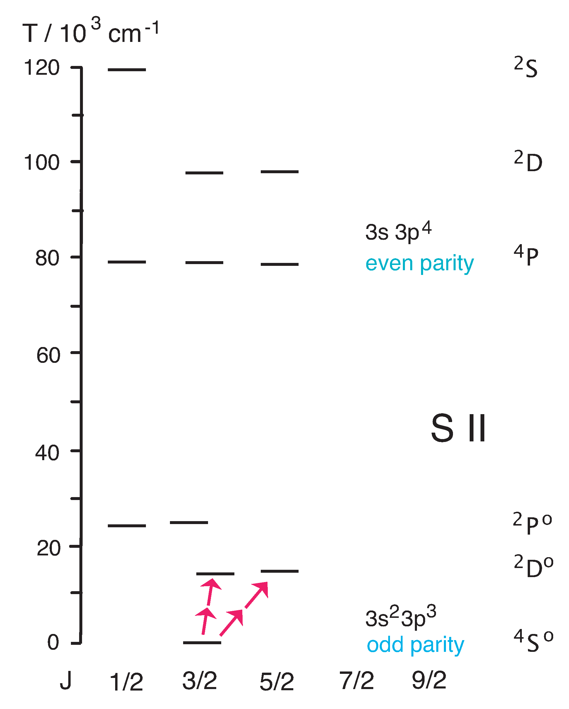
Figure 1.
Level structure and transitions in the 3s3p ground configuration of P-like S II (energy level positions not to scale), with wavelengths and approximate level lifetimes . All transitions are electric-dipole forbidden M1 or E2 transitions, respectively.
Figure 1.
Level structure and transitions in the 3s3p ground configuration of P-like S II (energy level positions not to scale), with wavelengths and approximate level lifetimes . All transitions are electric-dipole forbidden M1 or E2 transitions, respectively.

Figure 2.
Level structure and transitions in the 3s3p and 3s3p configurations of S II. The highest one of the 3s3p levels lies inside the range of 3s3p3d and 3s3p4ℓ levels (not shown here).
Figure 2.
Level structure and transitions in the 3s3p and 3s3p configurations of S II. The highest one of the 3s3p levels lies inside the range of 3s3p3d and 3s3p4ℓ levels (not shown here).

Figure 3.
Level structure (partial) of the 3s3p and 3s3p configurations of S II and Fe XII.

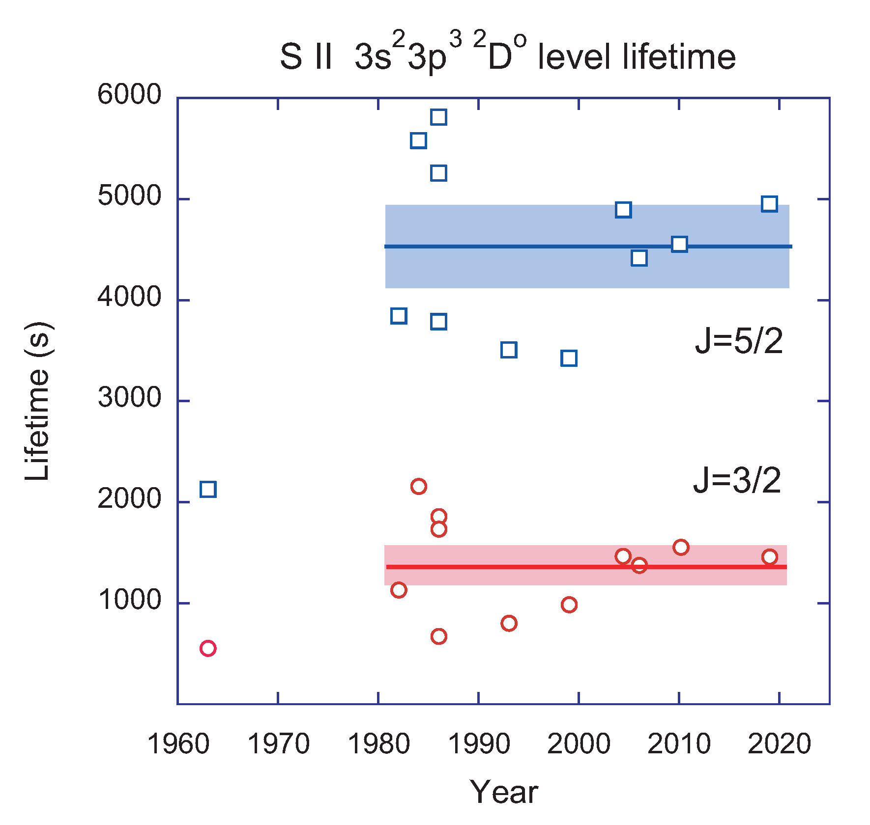
Figure 4.
Computed lifetimes of the 3s3p D levels of S II as a function of time of publication. The latest data point is from a data base without a creation date of this entry. The data entries can be identified from Table 1. The color bars indicate a visual mean value of the more recent results and a roughly ±10% interval for each of the levels.

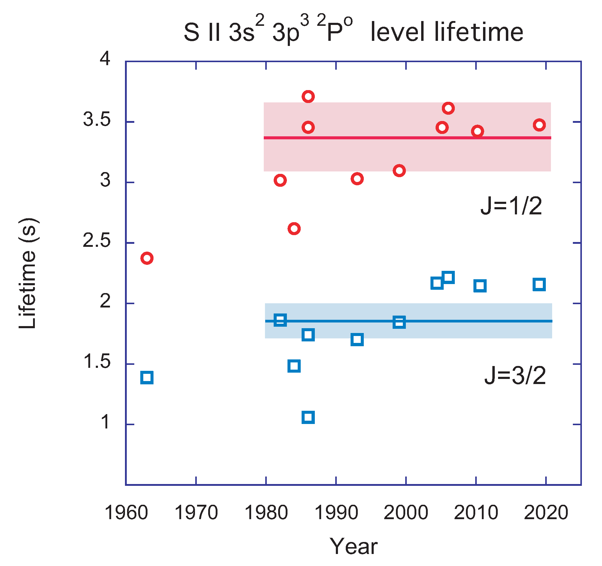
Figure 5.
Computed lifetimes of the 3s3p P levels of S II. The latest data point is from a data base without a creation date of this entry. The data entries can be identified from Table 2. The color bars indicate a visual mean value of the more recent results and a ±10% interval for each of the levels.

Figure 6.
Comparison of measured and computed lifetimes of the 3s3p D levels of highly charged P-like ions. The experiments (full symbols) used an electrostatic ion trap (Kingdon trap, KT) [15,16], the heavy-ion storage ring TSR [17,18], and an electron beam ion trap (EBIT) [19]. The reference computations were executed at the University of Puerto Rico (UPR) [18]. Other computational results: Mendoza & Zeippen [27], Huang [28], Biémont & Hansen [29], Kaufman & Sugar [30], NIST [21].

Figure 7.
S II level system and schematic of two-photon excitation of the 3s3p D levels from the ground state.
Figure 7.
S II level system and schematic of two-photon excitation of the 3s3p D levels from the ground state.

Figure 8.
S II level system and schematic of single-photon EUV laser excitation (wavelength 102.1 nm, blue lines) of the 3s 3p D levels and subsequent radiative decay (blue, lilac) to the levels of the ground configuration.
Figure 8.
S II level system and schematic of single-photon EUV laser excitation (wavelength 102.1 nm, blue lines) of the 3s 3p D levels and subsequent radiative decay (blue, lilac) to the levels of the ground configuration.

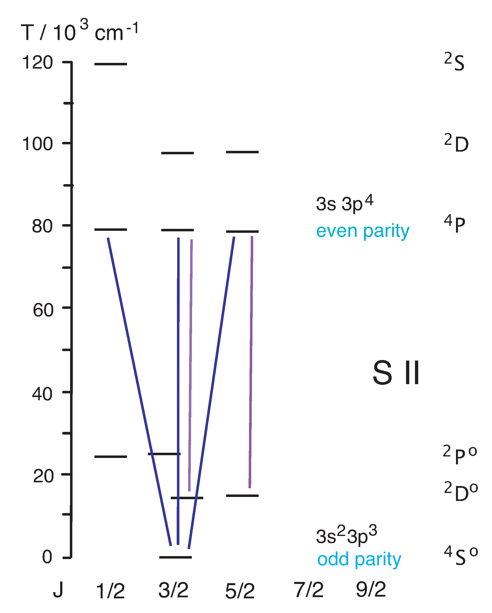
Figure 9.
The excitation of the 3s 3p P levels (blue lines) is followed by radiative decays to all levels of the ground configuration, including (lilac lines) the 3s 3p D levels. The decay branches to the doublet levels are weak.
Figure 9.
The excitation of the 3s 3p P levels (blue lines) is followed by radiative decays to all levels of the ground configuration, including (lilac lines) the 3s 3p D levels. The decay branches to the doublet levels are weak.

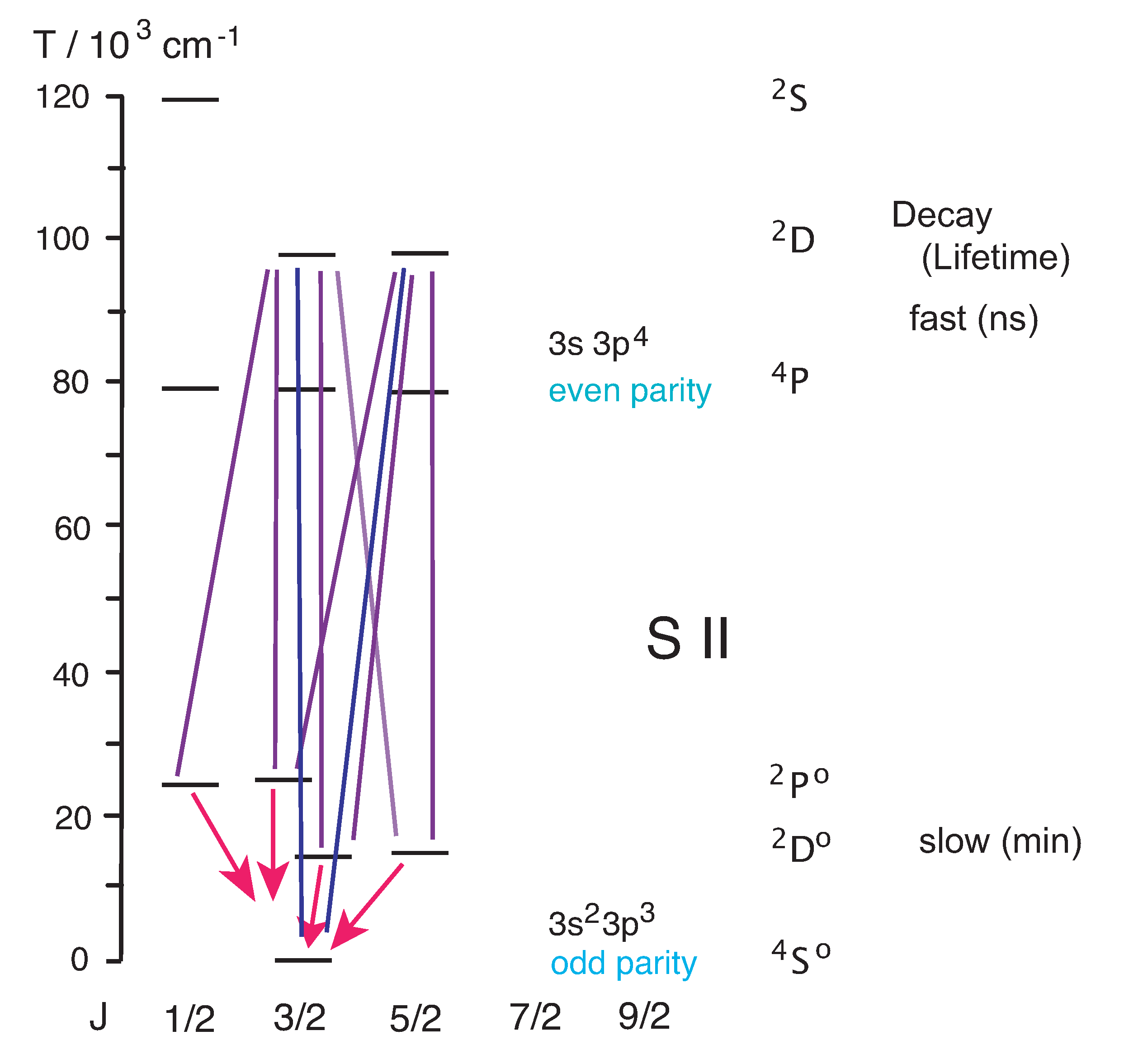
Figure 10.
Probing the 3s 3p D level populations by laser excitation ( ≈ 120 nm) to the 3s 3p D levels (green lines). The upper levels decay to all levels of the 3s 3p ground configuration, by emission of radiation at 82.3 nm, 120 nm, and 136 nm (violet and green lines).
Figure 10.
Probing the 3s 3p D level populations by laser excitation ( ≈ 120 nm) to the 3s 3p D levels (green lines). The upper levels decay to all levels of the 3s 3p ground configuration, by emission of radiation at 82.3 nm, 120 nm, and 136 nm (violet and green lines).


Table 1.
Total transition rate (+) and lifetime predictions for the 3s3p D levels of S II.
| Transition Rate | Lifetime | |||
|---|---|---|---|---|
| Ref. | A (s) | (s) | ||
| S–D | S–D | D | D | |
| Czyzak and Krueger 1963 [25] | 0.0018 | 0.00047 | 556 | 2128 |
| Mendoza and Zeippen 1982 [27] | 0.000882 | 0.00026 | 1134 | 3845 |
| Huang 1984 [28] | 0.0005 | 0.0002 | 2160 | 5583 |
| Kaufman and Sugar 1986 [30] | 0.000537 | 0.000264 | 1862 | 3788 |
| Froese Fischer and Godefroid 1986 [31] | ||||
| MCHF+BP | 0.0015 | 0.0002 | 675 | 5813 |
| MCDF | 0.0006 | 0.0002 | 1736 | 5258 |
| Keenan et al., 1993 [22] | 0.00124 | 0.000285 | 806 | 3509 |
| Fritzsche et al., 1999 [32] | 0.00101 | 0.000292 | 990 | 3427 |
| Irimia and Froese Fischer 2005 [33] | – | – | 1461 | 4936 |
| Froese Fischer et al., 2006 [34] | – | – | 1378 | 4419 |
| Tayal and Zatsarinny 2010 [35] | – | – | 1580 | 4550 |
| NIST 2019 [21] | 0.0007 | 0.0002 | 1462 | 4953 |
Table 2.
Lifetime predictions for the 3s3p P levels of S II.
| Lifetime | ||
|---|---|---|
| Ref. | (s) | |
| P | P | |
| Czyzak and Krueger 1963 [25] | 2.38 | 1.39 |
| Mendoza and Zeippen 1982 [27] | 3.02 | 1.86 |
| Huang 1984 [28] | 2.62 | 1.48 |
| Kaufman and Sugar 1986 [30] | 3.71 | 1.74 |
| Froese Fischer and Godefroid 1986 [31] | 3.46 | 1.06 |
| Keenan et al., 1993 [22] | 3.03 | 1.70 |
| Fritzsche et al., 1999 [32] | 3.10 | 1.85 |
| Irimia and Froese Fischer 2005 [33] | 3.46 | 2.16 |
| Froese Fischer et al., 2006 [34] | 3.62 | 2.22 |
| Tayal and Zatsarinny 2010 [35] | 3.39 | 2.14 |
| NIST 2019 [21] | 3.48 | 2.16 |
© 2020 by the author. Licensee MDPI, Basel, Switzerland. This article is an open access article distributed under the terms and conditions of the Creative Commons Attribution (CC BY) license (http://creativecommons.org/licenses/by/4.0/).
Share and Cite
MDPI and ACS Style
Träbert, E. A Laboratory Astrophysics Problem: The Lifetime of Very Long-Lived Levels in Low-Charge Ions. Atoms 2020, 8, 21. https://0-doi-org.brum.beds.ac.uk/10.3390/atoms8020021
AMA Style
Träbert E. A Laboratory Astrophysics Problem: The Lifetime of Very Long-Lived Levels in Low-Charge Ions. Atoms. 2020; 8(2):21. https://0-doi-org.brum.beds.ac.uk/10.3390/atoms8020021
Chicago/Turabian StyleTräbert, Elmar. 2020. "A Laboratory Astrophysics Problem: The Lifetime of Very Long-Lived Levels in Low-Charge Ions" Atoms 8, no. 2: 21. https://0-doi-org.brum.beds.ac.uk/10.3390/atoms8020021
Note that from the first issue of 2016, this journal uses article numbers instead of page numbers. See further details here.